Charmonium mass splittings at the physical point

Abstract:

We present results from an ongoing study of mass splittings of the lowest lying states in the charmonium system. We use clover valence charm quarks in the Fermilab interpretation, an improved staggered (asqtad) action for sea quarks, and the one-loop, tadpole-improved gauge action for gluons. This study includes five lattice spacings, 0.15, 0.12, 0.09, 0.06, and 0.045 fm, with two sets of degenerate up- and down-quark masses for most spacings. We use an enlarged set of interpolation operators and a variational analysis that permits study of various low-lying excited states. The masses of the sea quarks and charm valence quark are adjusted to their physical values. This large set of gauge configurations allows us to extrapolate results to the continuum physical point and test the methodology.

1 Objectives

The wealth of excited charmonium states discovered at the $B$ factories presents a challenge for interpretation (and, in some cases, confirmation). Some states could be spin-exotic hybrids and some “molecular” states. In principle, lattice QCD should provide a reliable guide to the interpretation of these states [1, 2, 3, 4, 5, 6]. For levels above the open charm threshold, the treatment of multihadronic scattering states presents a technical challenge. Other challenges are controlling heavy-quark discretization errors and, for some levels, including annihilation effects. Matching theory to experiment requires a relatively high degree of precision.

In the present study our more limited objective is to lay the foundation for future work by carrying out a high-precision study of the splittings of the low-lying states. Here we use clover charm quarks in the Fermilab interpretation [7]. To the extent we can reproduce the known splittings, we test the methodology. Validation of the method also gives confidence in other studies that use the same fermion formulations.

This work expands and extends our previous study [1] with clover (Fermilab) quarks and 2+1 flavors of asqtad sea quarks. We use a large variational basis of interpolating operators, and we extrapolate to zero lattice spacing and physical sea-quark masses.

2 Methodology

2.1 Gauge-field ensembles

We work with a large set of gauge-field ensembles generated in the presence of 2+1 flavors of asqtad sea quarks and a 1-loop tadpole improved gauge field [8, 9]. Parameters are listed in Table 1. These tuned values for the light quark masses are determined from chiral fits to masses and decay constants of the light pseudoscalar mesons [9].

Table 1: Parameters of the ensembles used in this study. Simulation light and heavy bare sea quark masses are denoted $m_{l}$ and $m_{h}$. Mass-independent, tuned physical bare masses are denoted $\hat{m}$ for degenerate up and down quarks and $m_{s}$ for strange. Also shown are the approximate lattice spacing, the lattice size, and the number of source times used (typically four per gauge configuration).

$\approx a$(fm)	$am_{l}$	$am_{h}$	$a\hat{m}$	$am_{s}$	size	sources
0.15	0.0097	0.0484	0.0015180	0.04213	$16^{3}\times 48$	2484
0.15	0.0048	0.0484	0.0015180	0.04213	$20^{3}\times 48$	2416
0.12	0.01	0.050	0.0012150	0.03357	$20^{3}\times 64$	4036
0.12	0.005	0.050	0.0012150	0.03357	$24^{3}\times 64$	3328
0.09	0.0062	0.031	0.0008923	0.02446	$28^{3}\times 96$	3728
0.09	0.0031	0.031	0.0009004	0.02468	$40^{3}\times 96$	4060
0.06	0.0036	0.018	0.0006401	0.01751	$48^{3}\times 144$	2604
0.06	0.0018	0.018	0.0006456	0.01766	$64^{3}\times 144$	1984
0.045	0.0024	0.014	0.0004742	0.01298	$64^{3}\times 192$	3204

2.2 Interpolating operators

As mentioned above, we use clover charm quarks with the Fermilab interpretation. Interpolating operators are classified according to their cubic group irreps and their $P$ and $C$ quantum numbers. We use a large basis of operators following Liao and Manke [10] and the JLab group [11]. Our operators are constructed from stochastic wall sources. Averaging over stochastic sources results in both local and smeared bilinears of the form

$${\cal O}_{i}(x)=\bar{q}(x)O_{i}q(x)\ \ \ {\cal O}^{\prime}_{i}(x)=\bar{q}(x)O_{i}Sq(x)\,,$$ (1)

where $O_{i}$ is one of several operators, as illustrated in Table 2, and $S$ represents covariant Laplacian smearing. (Only one width of smearing is included.) We do not include, however, any explicit open charm or charmonium/light-meson states in the list.

Table 2: Examples of charmonium interpolating operators used in this study. Here operators for the $T_{1}^{PC}$ irrep are shown. In the notation below, $\nabla_{i}$ generates a discrete covariant difference in direction $i$, $\mathbb{D}_{k}=|\varepsilon_{ijk}|\nabla_{i}\nabla_{j}$, and $\mathbb{B}_{i}=\varepsilon_{ijk}\nabla_{i}\nabla_{j}$.

$T_{1}^{--}$	$T_{1}^{+-}$	$T_{1}^{-+}$	$T_{1}^{++}$
$\gamma_{i}$	$\gamma_{4}\gamma_{5}\gamma_{i}$	$\gamma_{4}\nabla_{i}$	$\gamma_{5}\gamma_{i}$
$\gamma_{4}\gamma_{i}$	$\gamma_{5}\nabla_{i}$	$\varepsilon_{ijk}\gamma_{4}\gamma_{5}\gamma_{j}\nabla_{k}$	$\varepsilon_{ijk}\gamma_{j}\nabla_{k}$
$\nabla_{i}$	$\gamma_{4}\gamma_{5}\nabla_{i}$	$\varepsilon_{ijk}\gamma_{j}\mathbb{B}_{k}$	$\varepsilon_{ijk}\gamma_{4}\gamma_{j}\nabla_{k}$
$\varepsilon_{ijk}\gamma_{5}\gamma_{j}\nabla_{k}$	$|\varepsilon_{ijk}|\gamma_{4}\gamma_{5}\gamma_{j}\mathbb{D}_{k}$	$\varepsilon_{ijk}\gamma_{4}\gamma_{j}\mathbb{B}_{k}$	$|\varepsilon_{ijk}|\gamma_{5}\gamma_{j}\mathbb{D}_{k}$
$|\varepsilon_{ijk}|\gamma_{j}\mathbb{D}_{k}$	$\mathbb{B}_{i}$		$\gamma_{4}\mathbb{B}_{i}$
$|\varepsilon_{ijk}|\gamma_{4}\gamma_{j}\mathbb{D}_{k}$	$-$		$\varepsilon_{ijk}\gamma_{4}\gamma_{5}\gamma_{j}\mathbb{B}_{k}$
$\gamma_{5}\mathbb{B}_{i}$
$\gamma_{4}\gamma_{5}\mathbb{B}_{i}$

2.3 Variational determination of energy levels

In each channel (defined by the cubic group irrep and $P$ and $C$), we use the standard variational methodology [12, 13] for determining the lowest lying states. For interpolating operators $O_{i}$, we define the correlation matrix

$$C_{ij}(t)=\left\langle O_{i}(t)O_{j}(0)\right\rangle\,\,.$$ (2)

The goal is to determine, to good approximation, the energies $E_{n}$ in the spectral decomposition

$$C_{ij}(t)=\sum_{n}z_{in}z^{*}_{jn}\frac{\exp(-E_{n}t)}{2E_{n}}\,\,.$$ (3)

Ideally, the eigenvalues of the transfer matrix $T^{t-t_{0}}$ from time $t_{0}$ to time $t$ are $\lambda_{n}(t,t_{0})=\exp[-E_{n}(t-t_{0})]$. With a finite set of interpolating operators and a truncated list of energies, the eigenvalues receive contributions from higher states, which are modeled with [11]

$$\lambda_{n}(t,t_{0})=a_{0}\exp[-E_{n}(t-t_{0})]+a_{1}\exp[-E^{\prime}_{n}(t-t_{0})]+\ldots{}.$$ (4)

The lowest energy $E_{n}$ for each $n$ becomes an estimate of the $n$th excited state in that channel.

2.4 Scale and charm quark mass

The lattice scale is based on the Sommer $r_{1}$ parameter. It is determined in two steps. First, we have detailed measurements of its value in lattice units, $r_{1}/a$, from the heavy-quark potential. Then, $r_{1}$ itself is determined on the same lattice ensembles from a mass-independent, partially quenched, staggered $\chi$PT analysis of the light pseudoscalar masses and decay constants. That analysis used $f_{\pi}$, $M_{\pi}$, and $M_{K}$ to determine the physical bare light quark masses $\hat{m}$ and $m_{s}$ and $r_{1}=0.3117(22)\;$fm [14].

Once the lattice scale is known, we tune the charm quark mass by requiring that the kinetic mass $M_{2}$ of the $D_{s}$ meson, defined through the dispersion relation,

$$E_{D_{s}}({\bf p})=M_{1}+{\bf p}^{2}/(2M_{2})+\ldots{}\,,$$ (5)

matches the experimental value. In our implementation of the Fermilab method, we do not tune the value of $M_{1}$, the rest mass, however. Thus, the rest mass of the quark suffers from substantial discretization artifacts (except when $am_{c}\ll 1$). This contribution cancels, however, in the difference of two hadron rest masses. For that reason we report only level splittings below, e.g, $M_{1}(2S)-M_{1}(1S)$. For further discussion of this point, see Refs. [1, 7].

2.5 Sea-quark mass effects and continuum fit model

Although our gauge-field ensembles were generated in the presence of $2+1$ flavors of light sea quarks with fixed ratios of the bare quark masses, the initial estimate that set the simulation strange sea-quark mass was imprecise. In the worst case, on the 0.12 fm ensembles the strange sea quark was some 50% heavier than our best current estimate of its physical value in a mass-independent scheme (see Table 1). Thus, to extrapolate any of our measurements to the physical point, we include terms that model the dependence of the meson masses on sea-quark masses:

$$M=M_{0}+c_{1}(2x_{\ell}+x_{h})+c_{2}a^{2}\,,$$ (6)

where, in the notation of Table 1, $x_{\ell}=(m_{l}-\hat{m})/m_{s}$ and $x_{h}=(m_{h}-m_{s})/m_{s}$.

3 Results

1S hyperfine splitting

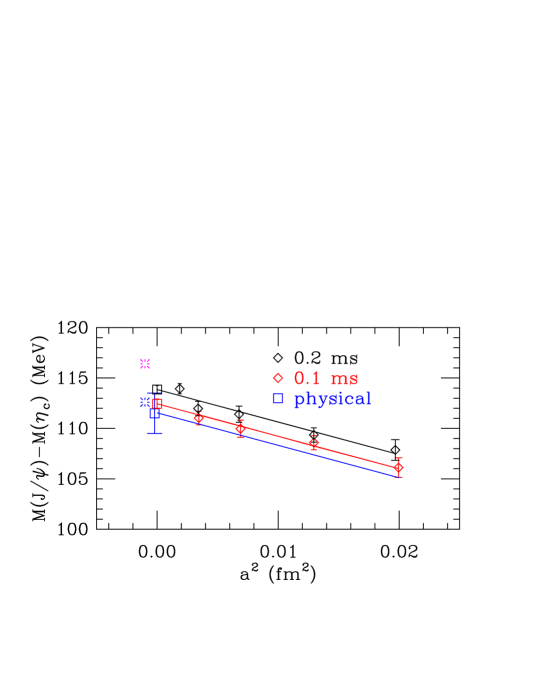
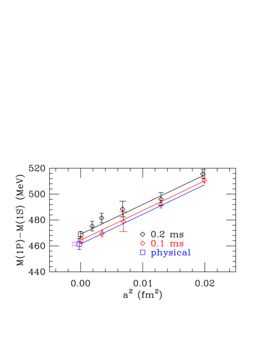
Figure 1: Left panel: $1S$ hyperfine splitting. Right panel: spin-averaged $1P-1S$ splitting. Errors on data points are statistical only. The blue square is the physical value including the $r_{1}$ scale error. The magenta burst (slightly displaced) is the PDG value. The blue burst is the recent BESIII result [15].

The hyperfine splitting of the $1S$ level provides a demanding test of the methodology [16]. The extrapolated result shown in Fig. 1 is compared with the current PDG value and the recent BESIII value[15]. Annihilation effects, which would decrease the splitting slightly [17] have not been included. The extrapolated error is $\pm 2$ MeV and appears to favor the BESIII value. The largest contribution to the uncertainty comes from our imperfect knowledge of $r_{1}$. In the determination of the hyperfine splitting, this uncertainty enters twice, first in setting the charm quark mass, and second, in comparing the splitting with the experimental value. In this quantity the error is amplified, not cancelled.

$1P-1S$ splitting

Results for the spin-averaged $1P-1S$ splitting are shown in Fig. 1. The error at the physical point (including the scale error) is $\pm 4$ MeV (1%).

$1P$ tensor and spin-orbit mass combinations

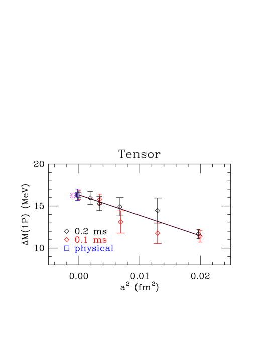
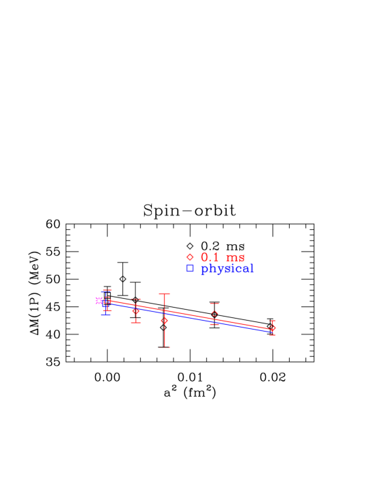
Figure 2: Left panel: $1P$ tensor mass combination. Right panel: $1P$ spin-orbit mass combination

The left panel of Fig. 2 shows the tensor mass combination

$$\frac{1}{9}[3M(\chi_{c1})-M(\chi_{c2})-2M(\chi_{c0})]$$

(extrapolated error $\pm 0.7$ MeV), and the right panel, the spin-orbit mass combination

$$\frac{1}{9}[5M(\chi_{c2})-2M(\chi_{c0})-3M(\chi_{c1})]$$

(extrapolated error $\pm 2$ MeV). In a heavy-quark expansion these mass splittings arise from the tensor and spin-orbit terms in the effective heavy-quark potential (quark model). These results are sensitive to discretization errors arising from those terms.

$2S$ states

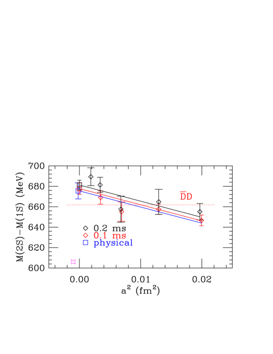
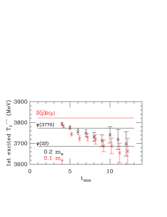
Figure 3: Left panel: Spin-averaged $2S-1S$ splittings. Note the experimental value (magenta burst) at the lower left. The physical open charm threshold is also shown. Right panel: $\psi(2S)$ level as a function of $t_{\rm min}$ at $a\approx 0.09$ fm. The full energy was reconstructed by adding the measured splitting to the experimental spin-averaged $1S$ level.

We overestimate considerably the splitting of the $2S$ and $1S$ levels, as shown in the left panel of Fig. 3. We get $675\pm 6$ MeV compared with the experimental value 606 MeV. The same problem was seen in [1] but with less clarity. Since the $2S$ levels are close to the open charm threshold, one may speculate that by not including an explicit open charm term in the variational mix, we cannot get a good representation of these states [18]. In support of this hypothesis, in the right panel of Fig. 3, we note that the splitting of the $\psi(2S)$ level from the $1S$ ground state shows a decreasing trend as $t_{\rm min}$, the minimum of the fit range in $\lambda_{n}(t)$, is increased. Indeed, if we set a higher $t_{\rm min}$ value for all lattice spacings and repeat the analysis, we get $651(12)$ MeV. Such behavior would result if a substantial open charm component is required but the transfer matrix has only a very weak mixing between closed and open charm. Such weak mixing has been known from string-breaking studies of the static potential [19, 20].

4 Conclusions and Outlook

We can reproduce the splittings of the lowest-lying charmonium levels to a precision of a couple of MeV. At this level of precision, however, we fail to reproduce the 2S-1S spin-averaged splitting with our set of interpolators. To complete the analysis we will develop a complete error budget. We will next try adding explicit open charm to the variational mix. We plan, also, to study bottomonium.

References

- [1] T. Burch et al. [Fermilab Lattice and MILC Collaborations], Phys. Rev. D 81, 034508 (2010) [arXiv:0912.2701 [hep-lat]].
- [2] G. Bali, S. Collins, S. Dürr, Z. Fodor, R. Horsley, C. Hoelbling, S. D. Katz and I. Kanamori et al., [arXiv:1108.6147 [hep-lat]].
- [3] L. Liu, S. M. Ryan, M. Peardon, G. Moir and P. Vilaseca, [arXiv:1112.1358 [hep-lat]].
- [4] Y. Namekawa et al. [PACS-CS Collaboration], Phys. Rev. D 84, 074505 (2011) [arXiv:1104.4600 [hep-lat]].
- [5] L. Liu, G. Moir, M. Peardon, S. M. Ryan, C. E. Thomas, P. Vilaseca, J. J. Dudek and R. G. Edwards et al., [arXiv:1204.5425 [hep-ph]].
- [6] D. Mohler, S. Prelovsek and R. M. Woloshyn, [arXiv:1208.4059 [hep-lat]].
- [7] A. X. El-Khadra, A. S. Kronfeld and P. B. Mackenzie, Phys. Rev. D 55, 3933 (1997) [arXiv:hep-lat/9604004].
- [8] T. Blum et al. [MILC Collaboration], Phys. Rev. D 55, 1133 (1997) [hep-lat/9609036]. C. W. Bernard et al. [MILC Collaboration], Phys. Rev. D 58, 014503 (1998) [hep-lat/9712010]. K. Orginos et al. [MILC Collaboration], Phys. Rev. D 59, 014501 (1999) [hep-lat/9805009]. J. F. Lagae and D. K. Sinclair, Phys. Rev. D 59, 014511 (1999) [hep-lat/9806014]. G. P. Lepage, Phys. Rev. D 59, 074502 (1999) [hep-lat/9809157]. K. Orginos et al. [MILC Collaboration], Phys. Rev. D 60, 054503 (1999) [hep-lat/9903032].
- [9] A. Bazavov et al., Rev. Mod. Phys. 82, 1349 (2010) [arXiv:0903.3598 [hep-lat]].
- [10] X. Liao and T. Manke, hep-lat/0210030 (2002).
- [11] J. J. Dudek, R. G. Edwards, N. Mathur and D. G. Richards, Phys. Rev. D 77, 034501 (2008) [arXiv:0707.4162 [hep-lat]].
- [12] C. Michael, Nucl. Phys. B 259, 58 (1985).
- [13] M. Lüscher and U. Wolff, Nucl. Phys. B 339, 222 (1990).
- [14] A. Bazavov et al. [Fermilab Lattice and MILC Collaborations], Phys. Rev. D 85, 114506 (2012) [arXiv:1112.3051 [hep-lat]].
- [15] M. Ablikim et al. [BESIII Collaboration], Phys. Rev. Lett. 108, 222002 (2012) [arXiv:1111.0398 [hep-ex]].
- [16] E. Follana (HPQCD Collaboration), \posPoS(Lattice 2010)305 (2010).
- [17] L. Levkova and C. DeTar, Phys. Rev. D 83, 074504 (2011) [arXiv:1012.1837 [hep-lat]].
- [18] G. S. Bali, S. Collins and C. Ehmann, Phys. Rev. D 84, 094506 (2011) [arXiv:1110.2381 [hep-lat]].
- [19] P. Pennanen et al. [UKQCD Collaboration], [hep-lat/0001015].
- [20] C. W. Bernard et al. [MILC Collaboration], Phys. Rev. D 64, 074509 (2001) [hep-lat/0103012].