Simultaneous first and second order percolation transitions in interdependent networks

Abstract

In a system of interdependent networks, an initial failure of nodes invokes a cascade of iterative failures that may lead to a total collapse of the whole system in a form of an abrupt first order transition. When the fraction of initial failed nodes $1-p$ reaches criticality, $p=p_{c}$, the abrupt collapse occurs by spontaneous cascading failures. At this stage, the giant component decreases slowly in a plateau form and the number of iterations in the cascade, $\tau$, diverges. The origin of this plateau and its increasing with the size of the system remained unclear. Here we find that simultaneously with the abrupt first order transition a spontaneous second order percolation occurs during the cascade of iterative failures. This sheds light on the origin of the plateau and on how its length scales with the size of the system. Understanding the critical nature of the dynamical process of cascading failures may be useful for designing strategies for preventing and mitigating catastrophic collapses.

I Introduction

Interdependent network systems attract a growing interest in the last years Laprie et al. (2007); Rosato et al. (2008); Panzieri and Setola (2008); Vespignani (2010); Buldyrev et al. (2010); Parshani et al. (2010a); Gao et al. (2011a); Leicht and D’Souza (2009); Morris and Barthelemy (2012); Saumell-Mendiola et al. (2012); Shao et al. (2011); Gao et al. (2011b); Huang et al. (2011); Gómez et al. (2013); Aguirre et al. (2013); Brummitt and R. M. D’Souza (2012); Bianconi (2013); Cellai et al. (2013); Radicchi and Arenas (2013); Li et al. (2012); Bashan et al. (2013). They represent real world systems composed of different types of interrelations, connectivity links between entities (nodes) of the same network to share supply or information and dependency links which represent a dependency of one node on the function of another node in another network. Consequently, failure of nodes may lead to two different effects: removal of other nodes from the same network which become disconnected from the giant component and failure of dependent nodes in other networks. The synergy between these two effects leads to an iterative chain cascading of failures. Buldyrev et al Buldyrev et al. (2010) show that, in a system of two fully interdependent random networks, when the fraction of failed nodes $1-p$ is smaller than a critical value, $p>p_{c}$, the cascading failures stop after some iterations and a finite fraction of the system, $P_{\infty}>0$, remains functioning and connected to the giant component. A larger initial damage, $p<p_{c}$, invokes a cascading failure that fragments the entire system and $P_{\infty}=0$. Thus, when $p$ approaches $p_{c}$ from above, the giant component, $P_{\infty}$, discontinuously jumps to zero in a form of a first order transition. The number of iterations in the cascade, $\tau$, diverges when $p$ approaches $p_{c}$, a behavior that was suggested as a clear indication for the transition point in numerical simulations Parshani et al. (2011).

Among the main features found are the collapse of the system with time (steps of cascading failures) in a plateau form (see Fig. 1), and the increase of the plateau length with the system size. Although this phenomena was observed in different models and in real data, its origin remained unclear Buldyrev et al. (2010). To understand the origin of this phenomena we focus on fully interdependent Erdős-Rényi (ER) networks. Surprisingly, we find here that during the abrupt collapse there appears a hidden spontaneous second order percolation transition that controls the cascading failures, as demonstrated in Fig. 1. We show here that this simultaneous second order phase transition, characterized by long branching trees near criticality, is the origin of the observed long plateau regime in the cascading failures and its dependence on system size. Moreover, the second order transition sheds light on the critical behavior observed in the collapse of real world systems such as the power law distribution of blackout sizes Carreras et al. (2004a); $\mathring{A}$. J. Holmgren and Molin (2006); Bakke et al. (2006); Ancell et al. (2005).

We also find, as a result of this new understanding, that even though the mean-field (MF) approximations are found to be accurate in predicting $p_{c}$ and $P_{\infty}$, it does not represent the dynamical process of cascading failures near criticality. This is since, the critical dynamics is strongly affected by random fluctuations due to the second order transition which are not considered in the MF approach. We study the effect of these fluctuations on the total number of iterations $\tau$ at criticality and find that its average and standard deviation scale as $N^{1/3}$, in contrast to the MF prediction of $\langle\tau\rangle\sim N^{1/4}$ Buldyrev et al. (2010). We present a theory for the dynamics at criticality, which explains the origin of this difference.

II Model of Interdependent Networks

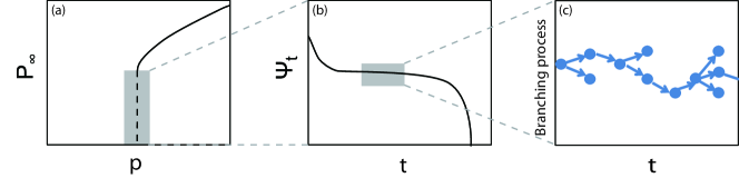
Figure 1: Demonstration of the simultaneous first and second order transitions in cascading failures of interdependent networks. At the critical point $p_{c}$, (a) the mutual giant component has a sudden jump to zero, while (b) the dynamical process of cascading failures is governed by a long plateau stage. In this plateau stage, a second order percolation occurs, which is (c) characterized by a random branching process at criticality, i.e., average branching factor is one (see Fig. 3).

In the fully interdependent networks model, $A$ and $B$ are two networks of the same size $N$. Each $A$-node $a_{i}$ depends on exactly one randomly-chosen $B$-node $b_{j}$, and $b_{j}$ also only depends on $a_{i}$. The initial attack is removing randomly a fraction $1-p$ of $A$-nodes in one network. Nodes in one network that depend on removed nodes in the other network are also removed, causing a cascade of failures. As nodes and edges are removed, each network breaks up into connected components (clusters). It is known that for single random networks, there is at most one component (giant component) which occupies a finite fraction of all $N$ nodes (see Cohen and Havlin (2010)). We assume that only nodes belonging to the giant component connecting a finite fraction of the network are still functional. Since the two networks have different topological structures, the failure will spread as a cascading process in the system Parshani et al. (2010b); Hu et al. (2013); Cellai et al. (2013). Here, one time step means that dependency failures and percolation failures occur at a given iteration in networks $A$ and $B$ respectively, and each network reaches a new smaller giant component.

The MF theory of this model with ER networks with average degrees $k_{A}$ and $k_{B}$ has been developed using generating functions of the degree distribution. This theory predicts the giant component size as a function of $p$, and accurately evaluate the first order phase transition threshold $p^{MF}_{c}$ for the infinite-size system. In fact, each realization in the simulation has its own critical threshold which we denote by $p_{c}$. In this paper, a new realization means that we generate networks $A$ and $B$ again, as well as the interdependency links, and then we perform the initial attack according to a new random attack order (see ). Note that for $N\to\infty$, $p_{c}$ values in single realizations are the same and equal to $p_{c}^{MF}$.

III Scaling Behavior in the Critical Dynamics

Here, we investigate the dynamics of the critical cascading failures for each single realization of a pair of finite coupled networks. For simplicity, networks $A$ and $B$ have the same average degree $k$. The value of $p_{c}$ of each realization, can be determined accurately by randomly removing nodes one by one until the system fully collapses.

Fig. 2 exhibits several realizations of simulations at $p_{c}^{MF}$. As seen at criticality, the total time $\tau$ has large fluctuations. Each realization has a stage of time steps (a plateau) where the giant component of network $A$ decreases very slowly. Before or after this plateau stage, the cascading failure process is much faster.

Fig. 2 and Fig. 2 show the scaling behaviors of the mean and the standard deviation of $\tau$ as a function of $N$ and $p-p_{c}$. In our simulations, we consider $p\leq p_{c}$, and only those realizations that fully collapse. We wish to understand how $N$ and $p-p_{c}$ affect the mean and the standard deviation of the total time $\tau$.

It can be seen from Fig. 2 that $\langle\tau\rangle$ increases with $N$ as $\langle\tau\rangle\sim N^{1/3}$ at $p=p_{c}$. However, when $p<p_{c}$, $\langle\tau\rangle$ becomes constant for large values of $N$. Thus, we assume the following scaling function,

$$\langle\tau\rangle\sim N^{1/3}\cdot f(u),$$ (1)

where $u=(p_{c}-p)\cdot N^{1/\alpha}$, and $f(u)$ is a function which satisfies: $f(u)\sim const.$ for $u<<1$, $f(u)\sim u^{-\alpha/3}$ for $u>>1$, and we determine $\alpha$ such that the best scaling occurs.

To test Eq. (1) and identify $\alpha$, we plot in Fig. 2 $\langle\tau\rangle/N^{1/3}$ versus $u$. We find that the best choice of $\alpha$ for obtaining a good scaling collapse is $\alpha=3/2$. In this way, we can see that the slope of each curve changes from $0$ to about $-1/2$ at $u=(p_{c}-p)\cdot N^{2/3}\approx 1$. Therefore, the scaling behavior of $\langle\tau\rangle$ for $N<N^{\ast}\sim(p_{c}-p)^{-3/2}$ is

$$\langle\tau\rangle\sim N^{1/3},$$ (2)

independent of $p$ (Fig. 2). This means that system sizes of $N<N^{\ast}$ are at criticality even though $p<p_{c}$. For $N>N^{\ast}$, $\langle\tau\rangle\sim N^{1/3}\cdot u^{-1/2}=(p_{c}-p)^{-1/2}$, independent of $N$ (Fig. 2) (non-critical behaviors). This yields the crossover $N^{\ast}\sim(p_{c}-p)^{-\alpha}=(p_{c}-p)^{-3/2}$, between the critical behavior for $N<N^{\ast}$ and non-critical for $N>N^{\ast}$. For $p\rightarrow p_{c}$, $N^{\ast}\rightarrow\infty$ and for all $N$ one observes the critical behavior. The crossover system size, $N^{\ast}$, can be regarded as a correlation size analogously to the correlation length in regular percolation Bunde and Havlin (1996); Stauffer and Aharony (1992).

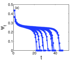
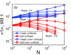
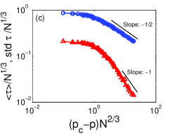
Figure 2: (Color online) a. Dynamical process of the giant component size $\psi_{t}$ of network $A$ in simulation at $p_{c}^{MF}$ (15 realizations). b. Scaling behavior of the mean (blue) and the standard deviation (red) of the total time $\tau$ at $p_{c}$ (critical) or below $p_{c}$ (non-critical) for each realization. Each curve here corresponds to a fixed value of $p$. c. The scaled version of (b). We consider for Fig. 2 the case $N=300\,000$ and $k=5$ with $15$ realizations. For Figs. 2 and 2, we have $k=5$ for the different $N$ values we analyzed. Each point here is the mean or the standard deviation over $200$ realizations of $N=10^{6}$, and order of $10^{4}$ realizations for $N\leq 300\,000$.

Fig. 2 also illustrates the scaling behaviors of the standard deviation, $\textup{{std}}(\tau)$. For $p=p_{c}$, we obtain $\textup{{std}}(\tau)\sim N^{1/3}$, i.e., it increases as the same rate as the mean. However, for $p<p_{c}$, the slope in the right tail of $\textup{{std}}(\tau)$ in Fig. 2 is about $-1/3$. Thus, we assume a scaling function for $\textup{{std}}(\tau)$:

$$\textup{{std}}(\tau)\sim N^{1/3}\cdot g(u),$$ (3)

where $u=(p_{c}-p)\cdot N^{1/\alpha}$, and $g(u)$ satisfies: $g(u)\sim const.$ for $u<<1$, and $g(u)\sim u^{-2\alpha/3}=u^{-1}$ for $u>>1$.

Fig. 2 shows that the scaling behavior of $\textup{{std}}(\tau)$ assumed in Eq. (3) is supported by simulations with the best choice $\alpha=3/2$ as for $\langle\tau\rangle$. The slope of the right tail in Fig. 2 is indeed $-1$. Thus, for $N<N^{\ast}$, we have the critical behavior: $\textup{{std}}(\tau)\sim N^{1/3}$; and for $N>N^{\ast}$, $\textup{{std}}(\tau)\sim N^{1/3}\cdot u^{-1}=N^{-1/3}(p_{c}-p)^{-1}$. Thus, we have the non-critical behavior also consistent with Fig. 2.

IV The Spontaneous Second Order Percolation Transition

Next we explore the mechanism behind the scaling behaviors near $p_{c}$. We show that it is due to a spontaneous second order percolation transition and explain the deviation from the MF theory. The failure size, $s_{t}$, the number of $A$-nodes that fail at time step $t$, during the plateau from the coupled networks system, is a zero fraction of the network size $N$. This is supported by simulations shown in Fig. 4. We regard each node that fails due to dependency at the beginning of the plateau stage as a root, $a_{i}$, of a failure tree (see Fig. 1). After that, the removal of each root $a_{i}$ will cause the failure of several other $A$-nodes due to percolation. Then, several $B$-nodes will fail due to dependency and percolation in network $B$. At the next time step, several $A$-nodes further fail due to dependency and percolation, which can be regarded as the result of the original removal of the root node $a_{i}$. Notice that the failures in network $A$ caused by removing different single nodes $a_{i}$ have very few overlaps due to the randomness and the large size of $N$. Therefore, we can describe the plateau stage by the growth of all these independent failure trees with the branching factor $\eta_{t}=s_{t+1}/s_{t}$.

Fig. 3 and Fig. 3 show the variation of $s_{t}$ and $\eta_{t}$ respectively in a typical realization that finally reached a total collapse. We observe that $\eta_{t}$ increases during the cascades from below $1$ to around $1$ (with some fluctuations) at the plateau, and finally to above $1$ when the system starts to collapse. The value of $\eta_{t}$ is smaller than $1$ in the beginning of the cascading process since the individual networks are still well connected and a large damage in one network leads to a smaller damage in the second network (see Fig. 3). As cascading progresses the value of $\eta_{t}$ increases since both networks become more dilute and a failure in one step leads to relatively higher damage in the next step (see Fig. 3). In this process the spontaneous behavior of $\eta_{t}$ generates a new phase transition. When $\eta_{t}$ approaches $1$ the system spontaneously enters a second order percolation transition where the cascading trees become critical branching processes (Bunde and Havlin (1996)) of typical length of $N^{1/3}$ as explained below. These long trees are the origin of the long plateau observed in Fig. 2.

The plateau stage starts when each of the $n$ failed nodes at iteration $T_{1}$ leads, in average (we refer to the fluctuations explicitly in the following), to failure of another single node (see ). This is a stable state, leading to the divergence of $\tau$ for $N\rightarrow\infty$. In a finite system of size $N$, however, the accumulated failures slightly reduce $p$ and the number of failures at each iteration gradually increases. This bias can be estimated by considering the percolation on single networks as follow.

At each time step $t$, the giant component size $\psi_{t}$ of network $A$ can be equivalently regarded as randomly attacking a fraction $1-p$ on a single ER network. This specific value of $p$, called the effective $p$ and denoted here by $p_{eff}$, can be obtained theoretically by solving the equation $\psi_{t}=p\cdot g(p)$, where $g(p)$ is the fraction of nodes in the giant component after randomly removing a fraction $p$ of nodes (see Buldyrev et al. (2010)).

Moreover, $\eta_{t}$ can be related to the branching factor for a single network. Consider randomly removing a fraction $1-p$ of nodes in an ER network, which makes some other nodes nonfunctional due to percolation, i.e., being disconnected from the giant component. Then, we randomly remove one more node within the giant component, and we use $\eta_{single}$ to denote the number of nodes that fail additionally due to percolation. Notice that $\eta_{single}$ is the branching factor for the additionally-removed node. Fig. 3 shows the relation between $p$ and $\eta_{single}$ for an ER network. Note that the branching factor diverges (for infinite systems) when $p\rightarrow p_{c}^{+}$, and converges to $0$ when $p\rightarrow 1$. Let $\tilde{p}$ be the critical value of $p$ where $\langle\eta_{single}\rangle=1$. Then we see from Fig. 3 that $\tilde{p}\approx 0.35$.

For two coupled ER networks, at each time step $t$ in the plateau stage, the difference between the giant components of networks $A$ and $B$ is small compared to the giant component sizes. Thus, each $A$($B$)-node that fails due to dependency can be approximately regarded as randomly removing one more node from the giant component of network $A$ ($B$). Therefore, $\eta_{t}\approx\langle\eta_{single}\rangle^{2}$ for the plateau stage. Notice that when $\langle\eta_{single}\rangle=1$, $\eta_{t}$ also equals to 1, and the threshold $\tilde{p}\approx 0.35$ is also valid for coupled ER networks. This can be seen in Fig. 3, which shows the evolution of $p_{eff}$ in the same realization of Fig. 3. We can see that the interaction between $p_{eff}$ and $\langle\eta_{t}\rangle$ is a determinate factor for the plateau stage. As shown in Fig. 3, when $p_{eff}$ gets smaller, $\eta_{t}$ increases to about $1$. This causes a range of time steps where $s_{t}$ is approximately a constant with some random fluctuations. Here, the random fluctuations of $\eta_{t}$ will determine the end of the cascading process, with or without a total collapse.

Based on these observations, we assume a random process of cascading failures starting at the beginning of the plateau state at $t=T_{1}$. Let $n=s_{T_{1}}$, which is also the number of independent failure trees, and consider time steps $T=t-T_{1}$. The variation of the failure sizes $s_{T}$ are determined by both the systematic bias and the random fluctuations. Here, the random fluctuations can be described by a Gaussian random walk from the value of $n$.

Assuming that $p_{eff}=\tilde{p}$, and $\eta_{T}=1$ at $T=0$, and $\eta_{T}$ decreases linearly when $p_{eff}$ increases near $\tilde{p}$: $\eta_{T}=1-C\cdot\Delta p_{eff}$. Here, $C$ is a positive constant, and $\Delta p_{eff}$ is the increment of $p_{eff}$ from $\tilde{p}$, which is approximately the variation of the giant component size of network $A$. Therefore, $\Delta p_{eff}=-\frac{\sum\limits_{i=0}^{T}s_{i}}{N}$. At $T=1$, we have $s_{1}=n\cdot(1-C\Delta p_{eff})=n\cdot(1+C\frac{n}{N})=n+\frac{C}{N}n^{2}$. At $T=2$, we have $s_{2}=s_{1}\cdot(1+\frac{C}{N}(n+s_{1}))$. After casting down small terms, we obtain $s_{2}=n+3\frac{C}{N}n^{2}$. Similarly, we can obtain at $T$:

$$s_{T}=n+\left(\sum\limits_{i=1}^{T}i\right)\cdot\frac{C}{N}n^{2}=n+\frac{T(T+1)}{2}\cdot\frac{C}{N}n^{2}.$$ (4)

Therefore, the order of the systematic bias of failure sizes from $T_{1}$ to $T_{2}$ is $\frac{n^{2}T^{2}}{N}$. If at some iteration the number of failures becomes zero the cascading process stops and the system survives. This can happen when $n-\sqrt{n}\sqrt{T}=0$, thus,

$$T_{stop}\sim\sqrt{n}.$$ (5)

If it does not stop, the cascading failures continue, and for large $T$ the bias will grow (faster than the fluctuations) leading to complete collapse. The balance between the bias and the fluctuations may continue as long as

$$\frac{n^{2}T^{2}}{N}\sim\sqrt{n}\sqrt{T}.$$ (6)

Equations (5) and (6) yield that $n\sim T\sim N^{1/3}$, which is supported by our simulation results in Fig. 2 showing $\langle\tau\rangle\equiv T\sim N^{1/3}$.

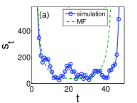
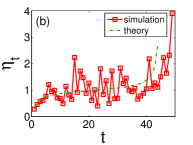
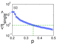
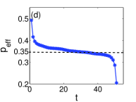
Figure 3: (Color online) a. The (blue) line with circles is the variation of failure sizes $s_{t}$ (only the plateau stage) for one realization in simulation. Here, $k=5$, $p=p_{c}^{MF}$ and $N=50\,000$. The (green) dashed dotted line shows $s_{t}$ for the MF case for $k=5$, $N=50\,000$, and $p=2.454/k$ slightly below $p^{MF}_{c}=2.4554/k$. b. The (red) line with rectangles shows the variation of the average branching factor $\eta_{t}$ for one realization in simulation. Here, $k=5$, $p=p_{c}^{MF}$ and $N=50\,000$. The (green) dashed dotted line shows $\eta_{t}$ of the analytic MF solution. Here, $k=5$, $N=50\,000$ and $p=2.4536/k$ below $p^{MF}_{c}$. In both (a) and (b), the MF values have similar behaviors as the simulation values, but the MF curves are smooth and show no fluctuations. c. The average branching factor $\langle\eta_{single}\rangle$ for different values of $p$ on a single ER network. Here, $k=5$, $N=250\,000$ for $3000$ realizations. A threshold $\tilde{p}$ where $\langle\eta_{single}\rangle=1$ can be observed at $p=\tilde{p}\approx 0.35$. d. The variation of the effective $p$ for one realization in the simulations. Here, $k=5$, $p=p_{c}^{MF}=2.4554/k$ and $N=50\,000$.

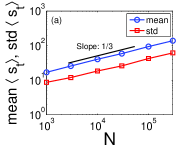
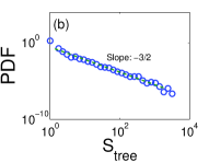
Figure 4: (Color online) a. Scaling results of the mean and the standard deviation of the average failure size $\langle s_{t}\rangle$ from $T_{1}$ to $T_{2}$, which is also the approximate number of branching processes for $p=p_{c}$ and $k=5$. Number or realizations is same as in Fig. 2. b. PDF of failure tree sizes $S_{tree}$ for the case $p=p_{c}$, $k=3$, $N=100\,000$ and 4537 trees in 80 realizations.

The above analysis also leads to the scaling law for the failure size at the beginning of the plateau stage: $n\sim N^{1/3}$. This is supported by simulations shown in Fig. 4, which exhibits the average failure size $\langle s_{t}\rangle$ along the plateau stage near criticality.

The critical behavior at the plateau is also represented in the distribution of failure tree sizes obtained in simulations shown in Fig. 4. Here, we determine the beginning and the end of the plateau (see ), and identify all $A$-nodes that fail due to dependency in each of the parallel failure trees. At each time step, the growth of each tree is determined by the branching factor $\eta_{t}$. On the plateau, most trees will rapidly die out, while several trees keep growing and become large. Fig. 4 displays the PDF of the tree size $S_{tree}$, which is the total number of nodes on a failure tree from the root to the time step where it terminates. We can see that the total tree size has a power-law distribution with a slope of approximately $-3/2$. It is interesting to note that such a distribution is associated with cluster size distributions in second order percolation transitions, see e.g., Bunde and Havlin (1996); Stauffer and Aharony (1992); Cohen and Havlin (2010) and obtained in classical models of self-organized criticality Carreras et al. (2004b); Chen et al. (2005); Nedic et al. (2006); Dobson et al. (2005, 2004). Notice also that the same critical exponent has been observed in real data Carreras et al. (2004a); $\mathring{A}$. J. Holmgren and Molin (2006); Bakke et al. (2006); Ancell et al. (2005).

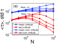
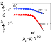
Figure 5: (Color online) a. Scaling behaviors of the mean (blue) and the standard deviation (red) of the total time $\tau$ at $p^{MF}_{c}=2.4554/k$ (critical) or below $p^{MF}_{c}$ (non-critical). Here, we consider $k=5$, and the number of realizations is $M=3000$. b. Scaled version of (a). Two more values of $p$ are included: $p=0.4908$ and $p=0.491$.

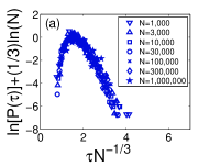
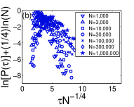
Figure 6: (Color online) a. Scaled PDF of $\tau$ using the exponent $1/3$ at $p=p_{c}$ for single realizations. Here, $k=5$, and the number of realizations is the same as in Fig. 2(b). b. Scaled PDF of $\tau$ using the exponent $1/4$.

V Relation between the Critical Scaling and the Mean-Field Case

Buldyrev et al. Buldyrev et al. (2010) found both analytically and numerically the scaling behavior $\langle\tau\rangle\sim N^{1/4}$ at $p^{MF}_{c}$, which is significantly different from the critical scaling result $N^{1/3}$ found here at $p_{c}$ of each realization. Fig. 5 shows the scaling behaviors of both $\langle\tau\rangle$ and $\textup{{std}}(\tau)$ at and below $p^{MF}_{c}$. As can be seen, the mean behavior is indeed consistent with the MF predictions of Buldyrev et al. (2010). We will explain in this section this seemingly discrepancy by analyzing the theoretical relationship between the scaling behaviors at $p_{c}$ of single realizations and at the MF prediction $p^{MF}_{c}$.

In Fig. 5, we observe the scaling rule of $\langle\tau\rangle$: $\langle\tau\rangle\sim N^{1/4}\cdot f(u)$, where, $u=(p^{MF}_{c}-p)\cdot N^{1/\alpha}$, and $\alpha=2$. Then, we have $f(u)\sim 1$ for $u\ll 1$, and $f(u)\sim u^{-1/2}$ for $u\gg 1$. Finally, for $N<N^{\ast}\sim(p_{c}-p)^{-3/2}$, $\langle\tau\rangle\sim N^{1/4}$, and for $N>N^{\ast}$, $\langle\tau\rangle\sim(p_{c}-p)^{-1/2}$. Compared with the scaling results for single realizations, Eqs. (1) and (2), the main difference is the exponent $1/4$ of the scaling of $\langle\tau\rangle$ with $N$. To further validate our new scaling law, $\langle\tau\rangle\sim N^{1/3}$ at $p=p_{c}$ of single realizations, we also compare in Fig. 6 the two scaling laws for the PDF of $\tau$: Fig. 6 presents the PDF of $\tau$ for different values of $N$ according to the scaling assumption $\tau\sim N^{1/3}$, whereas Fig. 6 gives the PDF of $\tau$ according to the scaling assumption $\tau\sim N^{1/4}$. As can bee seen from these figures, the assumption $\tau\sim N^{1/3}$ seems to better fit the scaling for single realizations, further supporting Eq. (2).

The origin of the MF observation, $\langle\tau\rangle\sim N^{1/4}$ and $\textup{{std}}(\tau)\sim N^{1/3}$ (see Fig. 5), which deviates from Eq. (2) for single realizations, can be explained by considering the fluctuations which do not appear in the MF case.

Given $\langle\tau\rangle\sim N^{1/3}$ at $p_{c}$, and $\langle\tau\rangle\sim(p_{c}-p)^{-1/2}$ when $p$ is below $p_{c}$, the scaling behavior at $p^{MF}_{c}$ can be regarded as the expectation of $\langle\tau\rangle$ below $p_{c}$:

$$\langle\tau\rangle_{MF}=\int^{\infty}_{0}\langle\tau\rangle\cdot D(x)dx,$$ (7)

where $x=p_{c}-p$, and $D(x)$ is its probability density. From the scaling results in Fig. 2, we know that $\langle\tau\rangle\sim N^{1/3}$, for $p_{c}-p<N^{-2/3}$ and $\langle\tau\rangle\sim(p_{c}-p)^{-1/2}$, for $p_{c}-p>N^{-2/3}$. We also assume that the value of $p_{c}$ follows a Gaussian distribution $N(p^{MF}_{c},\sigma^{2})$ (This is supported by the distribution of $p_{c}$ in simulations, see Fig. 7 in the Appendix.) above $p^{MF}_{c}$, where $\sigma\sim N^{-1/2}$. Therefore,

$$\langle\tau\rangle_{MF}=I_{1}+I_{2}\sim\int^{N^{-2/3}}_{0}N^{1/3}\cdot\frac{1}{\sqrt{2\pi}\sigma}\exp\left(-\frac{x^{2}}{2\sigma^{2}}\right)dx$$

$$+\int^{\infty}_{N^{-2/3}}x^{-1/2}\cdot\frac{1}{\sqrt{2\pi}\sigma}\exp\left(-\frac{x^{2}}{2\sigma^{2}}\right)dx.$$ (8)

Let $y=x\cdot\sqrt{N}$, which finally yields $I_{1}\sim N^{1/6}$ and $I_{2}\sim N^{1/4}$, from which follows $\langle\tau\rangle_{MF}=I_{1}+I_{2}\sim N^{1/4}$ for large $N$.

Similarly, we can also calculate the variance of $\tau$ using $\textup{{var}}(\tau)=\langle\tau^{2}\rangle-\langle\tau\rangle^{2}$, and then estimate the scaling result for the standard deviation at $p^{MF}_{c}$. We can finally obtain $\textup{{std}}(\tau)\sim N^{1/4}$, instead of $N^{1/3}$, seen in Fig. 5. The explanation of this deviation can be understood by performing accurate numerical integrals for the analogous Eq. (V) for the standard deviation. This accurate integration shows that for small values of $N$, the scaling of $\textup{{std}}(\tau)$ with $N$ can be approximated as $\textup{{std}}(\tau)\sim N^{1/3}$. However, for large $N$, the slope decreases to $N^{1/4}$. This might explain for the slope $1/3$ of $\textup{{std}}(\tau)$ at $p^{MF}_{c}$ observed in simulations, as shown in Fig. 5.

VI Summary

In this paper, we identified a spontaneous second order percolation transition occurring during the cascading failures which controls the first order abrupt transition. This spontaneous transition is characterized by cascading of failure trees whose size distribution is power law with an exponent $-3/2$ during the plateau stage. This explains the origin of the long plateau and its scaling with $N$ found in cascading process near the abrupt collapse of the coupled networks system. We also uncovered the theoretical relationship between the two seemingly contradictory scaling, $\langle\tau\rangle\sim N^{1/4}$ at the mean-field criticality and $\langle\tau\rangle\sim N^{1/3}$ at $p_{c}$ of single realizations, by considering the deviation of $p_{c}$ in different realizations.

VII Appendix

1. Distribution of $p_{c}$ around the mean-field prediction.

Fig. 7 shows the PDF of the normalized values of $p_{c}$: $p^{\prime}_{c}\equiv\frac{p_{c}-\langle p_{c}\rangle}{\textup{{std}}(p_{c})}$, compared with a standard Gaussian distribution. Here we can find that $p_{c}$ follows a Gaussian distribution around the MF prediction $p_{c}^{MF}$. This supports our assumption in the main text that $p_{c}$ follows a Gaussian distribution.

2. Effect of the randomness in network structures

In our simulations, there are two types of randomness in each realization: the structure of ER network and the random initial attack. We always change both the networks and the attack order at the beginning of each realization. However, when the network is large enough, the randomness of the network structure is not needed for our results. In Fig. 8, we compare the scaling behaviors of the total number of cascade $\tau$ in two cases: varying both the networks and the attack order, and varying only the attack order for a given realization. We find that they have very similar behavior.

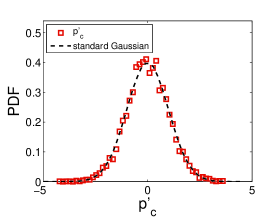
Figure 7: (Color online) PDF of the normalized $p_{c}$, $p^{\prime}_{c}$, for single realizations in simulations, compared with the standard Gaussian distribution. Here, $k=5$, $N=30\,000$ for $6000$ realizations. We see here that the value of $p_{c}$ follows quite well a Gaussian distribution.

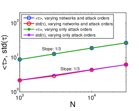
Figure 8: (Color online) Scaling behaviors of the mean and the standard deviation of the total time $\tau$ at $p_{c}$ for individual realizations. Two cases are compared here: in each realization, varying both the networks and the attack order, and only varying the attack order. We consider $k=5$ with $3000$ realizations for different $N$ values.

References

- Laprie et al. (2007) J. Laprie, K. Kanoun, and M. Kaniche, Lect. Notes Comput. Sci. 4680, 54 (2007).
- Rosato et al. (2008) V. Rosato, L. Issacharoff, F. Tiriticco, S. Meloni, S. De Porcellinis, and R. Setola, Int. J. Crit. Infrastruct 4, 63 (2008).
- Panzieri and Setola (2008) S. Panzieri and R. Setola, Int. J. Model. Ident. Contr. 3, 69 (2008).
- Vespignani (2010) A. Vespignani, Nature (London) 464, 984 (2010).
- Buldyrev et al. (2010) S. V. Buldyrev, R. Parshani, G. Paul, H. E. Stanley, and S. Havlin, Nature (London) 464, 1025 (2010).
- Parshani et al. (2010a) R. Parshani, S. V. Buldyrev, and S. Havlin, Phys. Rev. Lett. 105, 048701 (2010a).
- Gao et al. (2011a) J. Gao, S. V. Buldyrev, H. E. Stanley, and S. Havlin, Nature Physics 8, 40 (2011a).
- Leicht and D’Souza (2009) E. A. Leicht and R. M. D’Souza, “Percolation on interacting networks,” (2009), arXiv:0907.0894 .
- Morris and Barthelemy (2012) R. G. Morris and M. Barthelemy, Phys. Rev. Lett. 109, 128703 (2012).
- Saumell-Mendiola et al. (2012) A. Saumell-Mendiola, M. A. Serrano, and M. Boguñá, Phys. Rev. E 86, 026106 (2012).
- Shao et al. (2011) J. Shao, S. V. Buldyrev, S. Havlin, and H. E. Stanley, Phys. Rev. E 83, 036116 (2011).
- Gao et al. (2011b) J. Gao, S. V. Buldyrev, S. Havlin, and H. E. Stanley, Phys. Rev. Lett. 107, 195701 (2011b).
- Huang et al. (2011) X. Huang, J. Gao, S. V. Buldyrev, S. Havlin, and H. E. Stanley, Phys. Rev. E 83, 065101 (2011).
- Gómez et al. (2013) S. Gómez, A. Díaz-Guilera, J. Gómez-Gardeñes, C. J. Pérez-Vicente, Y. Moreno, and A. Arenas, Phys. Rev. Lett. 110, 028701 (2013).
- Aguirre et al. (2013) J. Aguirre, D. Papo, and J. M. Buldú, Nature Physics 9, 230 (2013).
- Brummitt and R. M. D’Souza (2012) C. D. Brummitt and E. A. L. R. M. D’Souza, Proc. Natl. Acad. Sci. 109, E680 (2012).
- Bianconi (2013) G. Bianconi, Phys. Rev. E 87, 062806 (2013).
- Cellai et al. (2013) D. Cellai, E. López, J. Zhou, J. P. Gleeson, and G. Bianconi, Phys. Rev. E 88, 052811 (2013).
- Radicchi and Arenas (2013) F. Radicchi and A. Arenas, Nature Physics 9, 717 (2013).
- Li et al. (2012) W. Li, A. Bashan, S. V. Buldyrev, H. E. Stanley, and S. Havlin, Phys. Rev. Lett. 108, 228702 (2012).
- Bashan et al. (2013) A. Bashan, Y. Berezin, S. V. Buldyrev, and S. Havlin, Nature Physics 9, 667 (2013).
- Parshani et al. (2011) R. Parshani, S. V. Buldyrev, and S. Havlin, Proc. Natl. Acad. Sci. 108, 1007 (2011).
- Carreras et al. (2004a) B. A. Carreras, D. E. Newman, I. Dobson, and A. B. Poole, IEEE Trans. Circuits Syst., I: Fundam. Theory Appl. 51, 1733 (2004a).
- . J. Holmgren and Molin (2006) . J. Holmgren and S. Molin, J. Infrastruct. Syst. 12, 243 (2006).
- Bakke et al. (2006) J. Bakke, A. Hansen, and J. Kertész, Europhys. Lett. 76, 717 (2006).
- Ancell et al. (2005) G. Ancell, C. Edwards, and V. Krichtal, in Electricity Engineers Association 2005 Conference: Implementing New Zealand s Energy Options (Aukland, New Zealand, 2005).
- Cohen and Havlin (2010) R. Cohen and S. Havlin, Complex Networks: Structure, Robustness and Function (Cambridge University Press, 2010).
- Parshani et al. (2010b) R. Parshani, C. Rozenblat, D. Ietri, C. Ducruet, and S. Havlin, Europhys. Lett. 92, 68002 (2010b).
- Hu et al. (2013) Y. Hu, D. Zhou, R. Zhang, Z. Han, C. Rozenblat, and S. Havlin, Phys. Rev. E 88, 052805 (2013).
- Note (1) We tested also by taking a few different realizations and keeping the network structures but changing only the attack order. The results have been found to be very similar, as seen in Fig. 8.
- Bunde and Havlin (1996) A. Bunde and S. Havlin, Fractals and Disordered Systems (Springer, 1996).
- Stauffer and Aharony (1992) D. Stauffer and A. Aharony, Introduction to Percolation Theory (Taylor & Francis, 1992).
- Note (2) In order to estimate the length of the plateau stage, we introduce a method to define the beginning, , and the end, , of the plateau in each realization. In Fig. 3, we find the time step of the first local minimum and of the last local minimum. Then, we define a threshold , which is twice the average failure size between these two minimums. This is because the values always have some random fluctuations above or below the mean value, which should be the same order as the mean. Therefore, we use twice the mean as the threshold for including such fluctuations. Then, we define and as the first time step and the last one where .
- Carreras et al. (2004b) B. A. Carreras, V. E. Lynch, I. Dobson, and D. E. Newman, Chaos 14, 643 (2004b).
- Chen et al. (2005) J. Chen, J. S. Thorp, and I. Dobson, Int. J. Electr. Power Energy Syst. 27, 318 (2005).
- Nedic et al. (2006) D. P. Nedic, I. Dobson, D. S. Kirschen, B. A. Carreras, and V. E. Lynch, Int. J. Electr. Power Energy Syst. 28, 627 (2006).
- Dobson et al. (2005) I. Dobson, B. A. Carreras, and D. E. Newman, Probab. Eng. Inform. Sc. 19, 15 (2005).
- Dobson et al. (2004) I. Dobson, B. A. Carreras, and D. E. Newman, in 37th Hawaii International Conference on System Sciences (Hawaii, 2004).