Charged Ising Model of Neutron Star Matter

Abstract

Background

The inner crust of a neutron star is believed to consist of Coulomb-frustrated complex structures known as “nuclear pasta” that display interesting and unique low-energy dynamics.

Purpose

To elucidate the structure and composition of the neutron-star crust as a function of temperature, density, and proton fraction.

Methods

A new lattice-gas model, the “Charged-Ising Model” (CIM), is introduced to simulate the behavior of neutron-star matter. Preliminary Monte Carlo simulations on $30^{3}$ lattices are performed for a variety of temperatures, densities, and proton fractions.

Results

Results are obtained for the heat capacity, pair-correlation function, and static structure factor for a variety of conditions appropriate to the inner stellar crust.

Conclusions

Although relatively simple, the CIM captures the essence of Coulomb frustration that is required to simulate the subtle dynamics of the inner stellar crust. Moreover, the computationally demanding long-range Coulomb interactions have been pre-computed at the appropriate lattice sites prior to the start of the simulation resulting in enormous computational gains. This work demonstrates the feasibility of future CIM simulations involving a large number of particles as a function of density, temperature, and proton fraction.

I Introduction

Neutron stars are compact objects with radii of the order of ten kilometers and masses comparable to that of the Sun. The solution of the Tolman-Oppenheimer-Volkoff (TOV) equations oppenheimer1 ; bombaci1 , which prescribes the structure of spherically symmetric, self-gravitating compacts object in hydrostatic equilibrium, provides information on the density profile of the star. Remarkably, the structure of neutron stars depends exclusively on the nuclear equation of state (EOS). Given the constraint of hydrostatic equilibrium, the density profile spans an enormous range of densities: from the extremely dilute crustal densities up to core densities that may greatly exceed nuclear-matter saturation density. Understanding what novels phases of matter emerge under these extreme conditions is both fascinating and unknown glendenning1 ; glendenning2 . Moreover, it represents one of the grand challenges in nuclear physics: “How does subatomic matter organize itself?” NucPhys2012 .

The highest density attained in the stellar core depends critically on the equation of state of neutron-rich matter. Although at such high densities the EOS is poorly constrained, it has been speculated that many exotic phases may emerge under such extreme conditions. These may include pion or kaon condensates Ellis:1995kz ; Pons:2000xf , strange quark matter Weber:2004kj , and color superconductors Alford:1998mk ; Alford:2007xm . It is also often assumed that the uniform core may have a non-exotic component consisting of neutrons, protons, electrons, and muons in chemical equilibrium. However, at densities of about half of nuclear-matter saturation density, the uniform core becomes unstable against cluster formation. At these “low” densities the average inter-nucleon separation increases to such an extent that it becomes energetically favorable for the system to segregate into regions of normal density (nuclear clusters) and regions of low density (neutron vapor). The transition region between the homogeneous and non-homogeneous phases constitutes the crust-core interface. It is the aim of this work to study the structure and composition of the crust-core interface where distance scales are such that the Coulomb and nuclear interactions become comparable in strength. Under these unique conditions neutron-rich matter becomes “frustrated”. Frustration, a prevalent phenomenon characterized by the existence of a very large number of low-energy configurations, emerges from the impossibility to simultaneously minimize all elementary interactions in the system. In the inner stellar crust this leads to a myriad of complex structures—collectively known as “nuclear pasta”—that are radically different in topology yet extremely close in energy. Moreover, due to the preponderance of low-energy states, frustrated systems display an interesting and unique low-energy dynamics. For example, it has been speculated that pasta formation could enhance the coherent scattering of neutrinos from such exotic structures. This could have important consequences on the supernova explosion mechanism and subsequent cooling dynamics watanabe1 ; horowitz1 ; margueron1 .

In this contribution we are interested in the equation of state of neutron-rich matter at densities of relevance to the inner stellar crust chamel1 ; bertulani1 . We will model this charge-neutral system in terms of its basic constituents, namely, neutrons, protons, and an ultra-relativistic Fermi gas of electrons. In particular, no ad-hoc biases will be introduced in regard to the structure of the exotic pasta shapes (i.e., whether they form droplets, rods, slabs, bubbles, etc.). Rather, we will allow the clustering to develop dynamically from an initial (random) configurations of nucleons. The aim of this work is to explore the dynamics of the system as a function of density, temperature, and proton fraction. Note that the original work by Ravenhall and collaborators was carried out at zero temperature in a mean-field approach ravenhall1 ; lorentz1 ; ravenhall2 . Recently, more sophisticated approaches—based on Monte Carlo and Molecular Dynamics simulations horowitz1 ; horowitz2 ; horowitz3 ; maruyama1 ; watanabe1 ; watanabe2 ; watanabe3 ; watanabe4 ; watanabe5 ; watanabe6 ; watanabe7 ; watanabe8 ; watanabe9 , a Dynamical-Wavelet approach sebille1 ; sebille2 ; sebille3 , relativistic mean-field calculations maruyama2 ; maruyama3 ; avancini1 ; avancini2 ; grill1 , and Skyrme-Hartree-Fock methods newton —have been implemented and have confirmed the existence of these exotic phases at very low temperatures and moderate proton fractions. However, given that chemical equilibrium suggests that the proton fraction in the inner stellar crust is very low—indeed, significantly lower than normally assumed—it has recently been put into question whether pasta formation is even possible in such proton-poor environments piekarewicz1 . Moreover, simulations at different temperatures are both critical and interesting because the long-range Coulomb interaction is responsible for the extreme fragility of crystals. That is, the melting (or charge-ordering) temperature in crystals $T_{c}$ is significantly smaller than the relevant Coulomb energy scale $E_{\rm Coul}\!=\!e^{2}/a$ (here $a$ is the lattice spacing). Such an energy mismatch introduces a large temperature gap ($k_{B}T_{c}\!<\!k_{B}T\!\ll\!E_{\rm Coul})$ where the system displays unconventional pasta-like behavior that reflects the strong frustration induced by the long-range interactions. In particular, condensed-matter simulations with long-range interactions have reported the opening of a pseudogap in the density of states in response to the strong frustration Pramudya2011 . This unconventional pseudogap region mediates the transition from the Wigner Crystal to the Fermi liquid. Interestingly enough, the pseudogap disappears for a system with only short-range interactions.

As an alternative to the numerically intensive Monte Carlo and Molecular Dynamics simulations, we introduce here the “Charged Ising Model” (CIM). The CIM is a lattice-gas model that while simple in its assumptions, retains the essence of Coulomb frustration. Numerical simulations based on this model are not as computationally demanding because the long-range Coulomb interaction, computed here exactly via an Ewald summation, may be pre-computed at the appropriate lattice sites and then stored in memory prior to the start of the simulation. This represents an enormous advantage when trying to simulate systems with a large number of particles as a function of temperature, density, and proton fraction. It is an important goal of this work to extend earlier (fixed-temperature) approaches by studying the thermal properties of the crust. Specifically, we rely on classical Monte Carlo simulations of the CIM to investigate phase transitions in stellar matter in the presence of Coulomb frustration. The CIM is reminiscent of an earlier approach developed in Refs. ising_star1 ; ising_star2 ; ising_star3 . Yet, it improves on it in two respects: (a) by including explicitly the isospin degree of freedom that is required for a proper treatment of asymmetric matter and (b) by using the Ewald summation to properly treat the long-range Coulomb interaction. Although limited in their treatment of quantum fluctuations, classical simulations like the ones proposed here are essential to uncover correlations that go beyond mean-field approaches. In particular, both spatial and thermal correlations—as embodied in the static structure factor and heat capacity—will be computed as a function of density, temperature, and proton fraction in the search of signatures of phase transitions.

The paper has been organized as follow. In Sec. II the CIM and the general framework will be introduced. Results from the simulations will be presented in Sec. III and then compared against previous findings reported in Ref. piekarewicz1 . Moreover, we will extend this earlier work by following the evolution of the pasta structures as a function of the temperature at fixed density and proton fraction. Finally, we offer our conclusions and suggestions for future work in Sec. IV.

II The CIM model: General framework

The main constituents of the stellar crust are neutrons, protons, and a background gas of neutralizing electrons. At the densities of relevance to the inner crust, the electrons may be treated as as an ultra-relativistic Fermi gas, namely, with a dispersion relation $\epsilon(p)\!=\!p$. Although the CIM presented here represents a simplification of the model first introduced in Ref. horowitz1 , it still retains the essence of Coulomb frustration, namely, competing interactions consisting of a short-range nuclear interaction and a long-range Coulomb potential. The CIM assumes that nucleons are allowed to occupy only the discrete sites of a three-dimensional cubic lattice of volume $V\!=\!L^{3}\!$ containing a total number of $S$ sites. The electrons on the other hand are assumed to provide a uniform neutralizing background.

The potential energy consists of a sum of a short-range interaction between nucleons and a long-range Coulomb interaction between protons and the uniform electron background. That is,

$$V_{\rm Total}=V_{\rm Nuclear}+V_{\rm Coulomb}\;.$$ (1)

For the short-range nuclear interaction the potential energy is assumed to be given by a sum of two-body terms that act exclusively over nearest neighbors. That is,

$$V_{\rm Nuclear}=\frac{1}{2}\sum_{\langle i,j\rangle}^{S}v_{ij}n_{i}n_{j}\,,$$ (2)

where $n_{i}\!=\!0,1$ denotes the occupation number of site $i$ and the “elementary” two-body interaction is given by

$$v_{ij}=\Big{(}b+c\tau_{i}\tau_{j}\Big{)}\,.$$ (3)

Here $\tau_{i}$ is the isospin of the nucleon occupying site $i$, with $\tau_{i}\!=\!+1$ for protons and $\tau_{i}\!=\!-1$ for neutrons. Note that the repulsive short-range nature of the NN interaction is simulated here by precluding the double occupancy of lattice sites. Also note that the two-body interaction is assumed to be isospin dependent to simulate quantum statistics. For example, in order to prevent pure neutron matter to be bound, the neutron-neutron interaction has to be made repulsive, namely, $v_{nn}\!=\!(b+c)\!>\!0$. Indeed, we now describe the procedure employed to fixed the two parameters $b$ and $c$. We assume that a completely filled lattice containing $A\!=\!S$ nucleons corresponds to nuclear-matter at saturation density. That is,

$$\rho_{{}_{0}}=\frac{A}{V}=\frac{1}{a^{3}}=0.16\,{\rm fm}^{-3}\,\implies a=1.842\,{\rm fm}.$$ (4)

For such a filled lattice the energy per nucleon of symmetric nuclear matter and pure neutron matter at saturation density are given by

$$\frac{E_{\rm SNM}}{A}=3(b-c)=-16.5\,{\rm MeV}\,,$$ (5a)

$$\frac{E_{\rm PNM}}{A}=3(b+c)=+15.5\,{\rm MeV}\,.$$ (5b)

This choice fixes the two model parameters to the following values:

$$b=-\frac{1}{6}\,{\rm MeV}=-0.167\,{\rm MeV}\,,$$ (6a)

$$c=+\frac{16}{3}\,{\rm MeV}=5.333\,{\rm MeV}\,,$$ (6b)

or equivalently,

$$v_{pn}=v_{np}=-5.500\,{\rm MeV}\,,$$ (7a)

$$v_{pp}=v_{nn}=+5.167\,{\rm MeV}\,.$$ (7b)

To illustrate the dynamics behind this very simple choice we display in Fig.1 results for the energy per nucleon of infinite nuclear matter (with the Coulomb interaction turned off and no electrons) as a function of both the filling fraction $\rho/\rho_{{}_{0}}\!=\!A/S$ and the proton fraction $x_{p}\!=\!Z/A$. Monte-Carlo simulations were performed on a cubic lattice of $S\!=\!(20)^{3}$ sites and at a temperature of $T\!\approx\!0$. Note that all simulations were started at the high temperature of $T\!=\!20\,{\rm MeV}$ and slowly cooled down to $T\!\approx\!0$ until the configuration was frozen. The EOS for symmetric nuclear matter ($x_{p}\!=\!0.5$) yields, by construction, a binding energy per nucleon at saturation density of $16.5\,{\rm MeV}$ and decreases to about $8\,{\rm MeV}$ at very low densities—corresponding to the binding energy of an isolated (symmetric) cluster. Note that in contrast to mean-field descriptions that assume nuclear matter to be uniform—and thus the energy to vanish at very low densities—the lattice-gas model takes full account (at least classically) of clustering correlations.

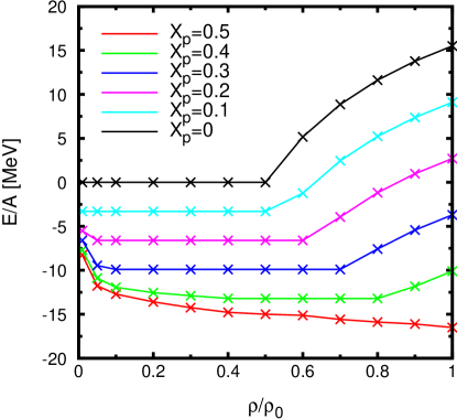
Figure 1: (color online) Energy per nucleon as a function of filling fraction $\rho/\rho_{{}_{0}}\!=\!A/S$ and proton fraction $x_{p}\!=\!Z/A$ for infinite nuclear matter. A proton fraction of $x_{p}\!=\!0.5$ represents symmetric nuclear matter whereas $x_{p}\!=\!0$ corresponds to pure neutron matter. Monte Carlo simulations were performed on a lattice with $S\!=\!(20)^{3}$ sites as the temperature $T\!\rightarrow\!0$.

At the other extreme ($x_{p}\!=\!0$) pure neutron matter is unbound at all densities and yields, by construction, an energy per neutron at saturation density of $15.5\,{\rm MeV}$; this corresponds to a symmetry energy at saturation density of $32\,{\rm MeV}$. Note that in the lattice model the energy of pure neutron matter vanishes at half filling (and below) as the lowest energy configuration consists of neutrons surrounded by empty sites.

For the emergence of frustration and the concomitant development of pasta structures, the Coulomb repulsion between protons is of critical importance. As mentioned earlier, at densities of relevance to the bottom layers of the inner crust (i.e., $10^{13}$-$10^{14}\,{\rm g/cm}^{3}$) the competition between the short-range nuclear attraction and the long-range Coulomb repulsion is the main driving force behind frustration. Whereas in earlier publications we adopted an approximate screened Coulomb interaction horowitz1 , more recently piekarewicz1 we have treated the problem exactly by means of an Ewald summation ewald1 . We follow the exact Ewald treatment here as well.

Using Ewald’s method we can cast the Coulomb potential as a sum of two-body interactions plus a constant term. That is,

$$V_{\rm Coulomb}=V_{0}+\frac{v_{{}_{0}}}{2}\sum_{i\neq j}^{S}u_{ij}n_{i}^{p}n_{j}^{p}\,,$$ (8)

where $n_{i}^{p}\!\equiv\!n_{i}(1\!+\!\tau_{i})/2$ denotes the proton occupation number of site $i$, $v_{{}_{0}}\!\equiv\!e^{2}/L$ sets the Coulomb energy scale, and $V_{0}$ is an overall constant piekarewicz1 . The dimensionless two-body potential $u_{ij}$ may be written in terms of short- and long-range contributions:

$$u_{ij} =\Big{[}u_{\rm sr}({\bf s}_{ij})+u_{\rm lr}({\bf s}_{ij})\Big{]}=\frac{{\rm erfc}(s_{ij}/s_{0})}{s_{ij}}$$

$$+\sum_{{\bf l}\neq 0}\frac{\exp(-\pi^{2}s_{0}^{2}\,l^{2})}{\pi l^{2}}\exp(-2\pi i{\bf l}\cdot{\bf s}_{ij})\;,$$ (9)

where ${\bf l}\!=\!(l_{x},l_{y},l_{z})$ represents a triplet of integers and ${\bf s}_{ij}$ is the separation between lattice sites $i$ and $j$ in dimensionless units. We now proceed with a brief explanation of the various terms; for a more detailed account see Ref. piekarewicz1 . The Coulomb potential is an interaction with no intrinsic scale. Ewald introduced a scale into the problem by adding $Z$ positive and $Z$ negative smeared charges at the exact location of each proton. It is both customary and convenient to introduce a gaussian charge distribution with a smearing parameter $a_{s}$; in the above expression $s_{0}\!=\!a_{s}/L$. The role of each negative charge is to fully screen the corresponding point proton charge over distances of the order of the smearing parameter. Thus, as long as $a_{s}$ is significantly smaller than the box length $L$, the resulting (screened) two-body potential [${\rm erfc}(s/\!s_{0})\!/\!s$] will become short ranged and thus amenable to be treated using the minimum-image convention ewald2 ; ewald3 . What remains then is a periodic system of smeared positive charges together with the neutralizing electron background. Whereas in configuration space this long-range contribution is slowly convergent, the great merit of the Ewald construction is that it can be made to converge rapidly if evaluated in momentum space, namely, as a Fourier sum. Indeed, the Fourier sum is rapidly convergent because (dimensionless) momenta ${\bf l}$ satisfying $ls_{0}\!\gg\!1$ make a negligible contribution to the Fourier sum. Hence, by suitably tuning the value of the smearing parameter, the evaluation of the Coulomb potential may be written in terms of two rapidly convergent sums; one in configuration space and one in momentum space piekarewicz1 . This is the enormous advantage of the Ewald construction. Another enormous advantage—now specific to the lattice model—is that one may pre-compute the two-body Coulomb interaction $u_{ij}$ for all different pairs of lattice sites and then stored them in an array for later retrieval during the simulation.

In what follows we employ a canonical ensemble to perform numerical simulations of a system consisting of $A$ nucleons, $Z\!=\!x_{p}A$, protons, and temperature $T$. A configuration in the system may be specified by a collection of $S$ occupation numbers ${\boldsymbol{\alpha}}\!=\!(\alpha_{1},\alpha_{2},\ldots,\alpha_{S})$, where at each site $\alpha_{i}\!=\!\{p,n,0\}$, depending on whether the site is occupied by either a proton or a neutron, or it remains vacant. Given that the potential energy is independent of momentum, the partition function for the system factors into a product of a partition function in momentum space—that has no impact in the computation of momentum-independent observables—times a coordinate space (or interaction) partition function of the form:

$${\mathcal{Z}(A,x_{p},T)}=\sum_{\boldsymbol{\alpha}}\exp\Big{(}\!-\!\beta\,V_{\rm Total}({\boldsymbol{\alpha}})\Big{)}\;,$$ (10)

where $\beta\!=\!(k_{B}T)^{-1}$ is the inverse temperature. In turn, the expectation value of any momentum-dependent observable ${\mathcal{O}}$ may be estimated by performing the appropriate statistical average. That is,

$$\langle{\mathcal{O}}\rangle=\sum_{\boldsymbol{\alpha}}{\mathcal{O}}({\boldsymbol{\alpha}})P_{\boldsymbol{\alpha}}(T)\;,$$ (11)

where $P_{\boldsymbol{\alpha}}(T)$ represents the probability of finding the system in a given configuration $\boldsymbol{\alpha}$. In the canonical ensemble such a probability is proportional to the properly normalized Boltzmann factor:

$$P_{\boldsymbol{\alpha}}(T)=\frac{\exp\Big{(}\!-\!\beta\,V_{\rm Total}({\boldsymbol{\alpha}})\Big{)}}{\mathcal{Z}(A,x_{p},T)}\;.$$ (12)

Given that the momentum-independent interactions have no impact on the kinetic energy of the system, the expectation value of the kinetic energy reduces to a sum of a classical contribution for the nucleons and a quantum contribution for the electrons. That is,

$$\langle K\rangle=\frac{3}{2}Ak_{B}T+\frac{3}{4}Zk_{\rm F}\left[1+\frac{2\pi^{2}}{3}\left(\frac{T}{T_{\rm F}}\right)^{2}\right]\;,$$ (13)

where $k_{\rm F}\!=\!k_{B}T_{\rm F}$ is the electronic Fermi momentum. The total energy of the system is then given by

$$\langle E(A,x_{p},T)\rangle=\langle K(A,x_{p},T)\rangle+\langle{V_{\rm Total}(A,x_{p},T)}\rangle\;.$$ (14)

We note that the sum over ${\boldsymbol{\alpha}}$ in Eq. (11) runs over a total number of configurations given by

$$C(A,Z)=\frac{S!}{Z!(A-Z)!(S-A)!}\;.$$ (15)

This number becomes astronomical even for systems of moderate size. Thus, to properly sample the statistical ensemble, we rely on a Metropolis Monte-Carlo algorithm metropolis1 to generate configurations distributed according to Eq. (12). Given that the kinetic energy of the system corresponds to that a classical ideal gas of nucleons and an ultra-relativistic Fermi gas of electrons, their contribution to the heat capacity is both known and smooth. Thus, any non-analytic behavior associated with the existence of a phase transition must arise from the interactions. For example, in the case of the heat capacity the potential energy contribution will be estimated from the fluctuations in the potential energy. That is,

$$\frac{C_{\rm v}}{k_{\rm B}}=\frac{3}{2}A+\pi^{2}Z\left(\frac{T}{T_{\rm F}}\right)+\frac{\langle V_{\rm Total}^{2}\rangle-\langle V_{\rm Total}\rangle^{2}}{(k_{\rm B}T)^{2}}\;.$$ (16)

Whereas the heat capacity accounts for the mean-square energy fluctuations—which diverge near phase transitions—the static structure factor $S({\bf k})$ provides a complimentary observable associated with the mean-square density fluctuations fetter1 . Moreover, $S({\bf k})$ is intimately related to a quantity particularly suitable to be modeled in computer simulations, namely, the pair-correlation function $g({\bf r})$. Indeed, $S({\bf k})$ and $g({\bf r})$ are simply Fourier transforms of each other. The pair-correlation function $g({\bf r})$ is particularly simple to simulate as it represents the probability of finding a pair of particles separated by a fixed distance ${\bf r}$. For a system containing $N$ particles and confined to a simulation volume $V$, $g(r)$ may be computed exclusively in terms of the instantaneous positions of the particles. That is,

$$g({\bf r})=1+\frac{V}{N(N-1)}\Big{\langle}\sum_{i\neq j}\delta({\bf r}-{\bf r}_{ij})\Big{\rangle}\;,$$ (17)

where ${\bf r}_{ij}\!=\!{\bf r}_{i}\!-\!{\bf r}_{j}$ and the “brackets” represent an ensemble average. Note that g(r) is normalized to $1$ at very large distances. Whereas for a uniform fluid the one-body density is constant, interesting two-body correlations emerge as a consequence of interactions. For example, the characteristic short-range repulsion of the $NN$ interaction precludes particles from approaching each other. This results in a pair-correlation function that vanishes at short separations. In the particular case of the CIM, this short-range repulsion is enforced by precluding two nucleons from occupying the same site. The static structure factor is obtained from the pair-correlation function through a Fourier transform. That is vesely1 ,

$$S({\bf k})=1+\frac{N}{V}\int d^{3}r\Big{(}g({\bf r})-1\Big{)}{\Large{e}}^{-i{\bf k}\cdot{\bf r}}\;.$$ (18)

Given that the static structure factor accounts for the mean-square density fluctuations in the ground state, it becomes a particularly useful indicator of the critical behavior associated with phase transitions—which themselves are characterized by the development of large (i.e., macroscopic) fluctuations. Indeed, the spectacular phenomenon of “critical opalescence” in fluids is the macroscopic manifestation of abnormally large density fluctuations—and thus abnormally large light scattering—near a phase transition pathria1 . In this regard, the static structure factor at zero-momentum transfer provides a unique connection to the thermodynamics of the system pathria1 . That is,

$$S({\bf k}\!=\!0)=\frac{\langle N^{2}\rangle-\langle N\rangle^{2}}{\langle N\rangle}=\frac{\langle N\rangle k_{B}T}{V}\kappa_{T}\;,$$ (19)

where $\kappa_{T}$ is the isothermal compressibility of the system. The isothermal compressibility is reminiscent of the heat capacity [Eq. (16)] that accounts for energy rather than density fluctuations. As such, they both play a critical role in identifying the onset of phase transitions.

As mentioned earlier, the various configurations of the system will be generated via a Metropolis Monte-Carlo algorithm with a weighting factor determined by the total potential energy of the CIM [see Eq. (12)]. The Metropolis algorithm is very well known metropolis1 ; vesely1 , so we only provide a brief review of those parts of relevance to our implementation. In particular, all Monte-Carlo moves must be consistent with the specified baryon number $A$ and proton fraction $x_{p}$. Thus, given a current configuration ${\boldsymbol{\alpha}}$, we propose a move to a new configuration ${\boldsymbol{\alpha}^{\prime}}$ by selecting two lattice sites ($i$ and $j$) at random and then simply exchange their occupancies (i.e., $\alpha_{i}\!\leftrightarrow\!\alpha_{j}$). This move ensures that both the baryon number the proton fraction are conserved during the simulation. The new configuration is accepted provided

$$\frac{P_{\boldsymbol{\alpha}^{\prime}}(T)}{P_{\boldsymbol{\alpha}}(T)}>{\rm rand}\;,$$ (20)

where ${\rm``rand"}$ is a random number between 0 and 1 drawn from a uniform distribution. Otherwise, the move is rejected and the original configuration ${\boldsymbol{\alpha}}$ is kept.

Initially, the lattice is populated by placing $Z\!=\!x_{p}A$ protons and $N\!=\!A\!-\!Z$ neutrons at random throughout the $S$ lattice sites. Given that each lattice site is occupied by at most one nucleon, a total of $S\!-\!A$ sites remain empty. The simulation starts by thermalizing the system at a temperature that is significantly higher than the target temperature $T$; this prescription prevents the system from getting trapped in a local minimum. Once the system is properly thermalized at the higher temperature, a very slow cooling schedule is enforced until the desired temperature $T$ is reached. Note that without a proper cooling schedule, a system that should crystallize at low temperature may end up resembling an amorphous solid. Once the system reaches the target temperature $T$, one proceeds to accumulate statistics in order to compute the thermal averages for a variety of physical observables. However, a strong correlation is likely to exist between two neighboring configurations ${\boldsymbol{\alpha}}$ and ${\boldsymbol{\alpha}}^{\prime}$ since they differ by (at most) the permutation of two occupation numbers. This correlations can significantly bias the results and may lead to an improper estimate of the Monte Carlo errors. To prevent this situation from developing, one selects uncorrelated events by calculating the normalized auto-correlation function of a suitable observable ${\cal O}$. For a large sequence of configurations $\{{\boldsymbol{\alpha}}_{1},{\boldsymbol{\alpha}}_{2},\ldots\}$, the auto-correlation function of ${\cal O}$ is defined by the following expression:

$$f\!_{{}_{\cal O}}\!(m)=\frac{\sum_{n=1}\Big{(}{\cal O}_{n}\!-\!\langle{\cal O}\rangle\Big{)}\Big{(}{\cal O}_{n+m}\!-\!\langle{\cal O}\rangle\Big{)}}{\sum_{n=1}\Big{(}{\cal O}_{n}\!-\!\langle{\cal O}\rangle\Big{)}^{2}}\;,$$ (21)

where ${\cal O}_{n}\!\equiv\!{\cal O}({\boldsymbol{\alpha}}_{n})$. The decorrelation “time” $\tau$ is defined by the condition $f\!_{{}_{\cal O}}\!(\tau)\!=\!0.1$. In Fig. 2 we display the auto-correlation function for the total potential energy $V_{\rm Total}$ for a filling fraction $A/S\!=\!0.2$, a proton fraction of $x_{p}\!=\!0.3$, and temperatures of $T\!=\!10$ MeV and $T\!=\!15$ MeV. At the lower temperature it becomes more difficult to explore the full energy landscape, thereby resulting a in a longer decorrelation time. For this particular case, $\tau_{{}_{\!10}}\!=\!7,218$ and $\tau_{{}_{\!15}}\!=\!5,550$. In what follows, all our results are reported with a proper treatment of Monte Carlo errors.

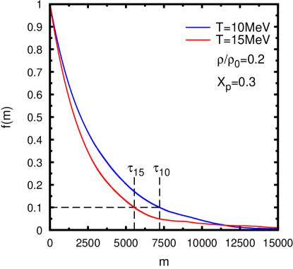
Figure 2: The auto-correlation function for the total potential energy at fixed density, fixed proton fraction, and two values of the temperature. The decorrelation time $\tau$ is defined by the condition $f(\tau)\!=\!0.1$.

III Results

We start this section by providing a baseline CIM calculation that aims to reproduce the results reported recently in Ref. piekarewicz1 . Recall that in Ref. piekarewicz1 the temperature was fixed at $T\!=\!1$ MeV in order to simulate the quantum zero-point motion. It is the goal of our present lattice-gas simulation to improve on such a work by examining the role of the temperature on the structure and dynamics of the inner stellar crust. Ultimately then, this sort of simulations will help us explore the phase diagram as a function of temperature, density, and proton fraction.

Given that the static structure factor at zero momentum transfer accounts for density fluctuations [see Eq. (19)], we begin this section by displaying in Figs. 3-6 pair correlations functions and static structure factors for neutrons and protons at a fixed temperature of $T\!=\!1$ MeV. Note that because of the discrete nature of the lattice, all distances between sites are “quantized”. Moreover, due to the periodicity of the lattice, the allowed values of the momenta are given as follows:

$${\bf k}=\frac{2\pi}{L}{\bf l}\quad(l_{i}=0,1,\ldots,S_{i}\!-\!1)\;,$$ (22)

where $S_{x}\!=\!S_{y}\!=\!S_{z}\!=\!S^{1/3}$.

Results are presented as a function of the proton fraction for a lattice of $S\!=\!(30)^{3}$ sites, and a filling fraction of $\rho/\rho_{{}_{\!0}}\!=\!A/S\!=\!0.1875$ (or $A\!\simeq\!5,000$ nucleons). The pair correlation function is characterized by a set of discrete peaks at the allowed distances on the lattice. For example, at this relatively low filling fraction, the dynamics favors the formation of neutron-rich clusters immersed in a dilute neutron vapor (see Fig. 11). Given that the neutron-proton interaction is attractive, nucleons organize themselves within a cluster by occupying alternating lattice sites. Thus, the closest distance between nucleons of the same species is $r_{\rm min}\!=\!\sqrt{2}a\!=\!2.605\,{\rm fm}$, where $a\!=1.842\,{\rm fm}$ is the lattice spacing [see Eq. (4)]. The largest peak in both Figs. 3 and 4 reflect this behavior. In the case of protons—where no dilute vapor is formed—other peaks corresponding to more distant protons are clearly discernible at distances of $2a\!=\!3.684$, $\sqrt{6}a\!=\!4.512$, $\sqrt{8}a\!=\!5.210$, $\sqrt{10}a\!=\!5.825,\ldots$ In the case of neutrons, the existence of a dilute neutron vapor gives rise to additional peaks and to significant pair-correlation strength at larger distances.

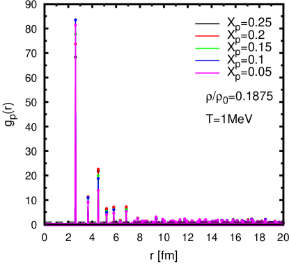
Figure 3: Proton pair correlation function for different proton fractions at a fixed density of $\rho/\rho_{{}_{0}}\!=\!0.1875$ and a temperature of $T\!=\!1$ MeV.

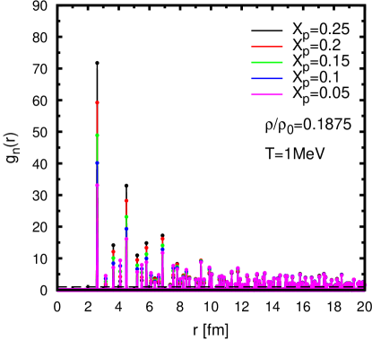
Figure 4: Neutron pair correlation function for different proton fractions at a fixed density of $\rho/\rho_{{}_{0}}\!=\!0.1875$ and a temperature of $T\!=\!1$ MeV.

The corresponding static structure factors for both protons and neutrons are shown in Figs. 5 and 6, respectively. Our results reproduce qualitatively those reported in Ref. piekarewicz1 . That is, $S(k)$ displays a prominent peak that becomes progressively higher with increasing proton fraction. The peak in $S(k)$ occurs at a momentum transfer $k$ for which the probe (e.g., electrons in the case of protons and neutrinos in the case of neutrons) can most efficiently scatter from the density fluctuations in the system. In particular, if the wavelength of the probe is large as compared with the size of the pasta structures, the scattering may be coherent. This can significantly enhance the response or, equivalently, significantly reduce the electron/neutrino mean-free path. Finally, as in Ref. piekarewicz1 , there is no visible enhancement in $S(k)$ at zero momentum transfer as would be expected from the putative phase transition from a Wigner Crystal to a pasta phase.

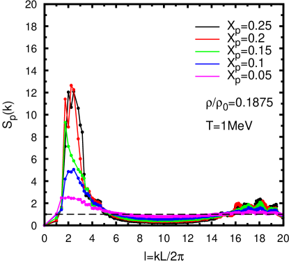
Figure 5: Proton static structure factor for different proton fractions at a fixed density of $\rho/\rho_{{}_{0}}\!=\!0.1875$ and a temperature of $T\!=\!1$ MeV.

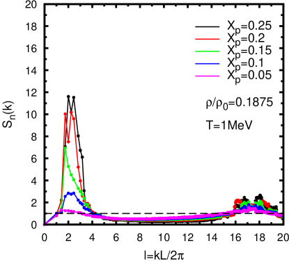
Figure 6: Neutron static structure factor for different proton fractions at a fixed density of $\rho/\rho_{{}_{0}}\!=\!0.1875$ and a temperature of $T\!=\!1$ MeV.

Although it is gratifying that the CIM reproduces the trends reported in Ref. piekarewicz1 , an important goal of the present work is to explore the evolution of the system—particularly the dissolution of the pasta—as a function of temperature. In analogy to the static structure factor that captures the density fluctuations in the system, we now examine thermal fluctuations through a study of the heat capacity [see Eq. (16)]. We start by displaying in Figs. 7-10 the neutron and proton pair correlation functions and corresponding static structure factors at a fixed density of $\rho/\rho_{{}_{0}}\!=\!0.2$, a fixed proton fraction of $x_{p}\!=\!0.3$, and for temperatures ranging from $T\!=\!1\,{\rm MeV}$ to $T\!=\!6\,{\rm MeV}$. In particular, note that under these conditions of density and proton fraction—and at the low temperature of $T\!=\!1\,{\rm MeV}$—the existence of a pasta phase has been well established horowitz1 ; watanabe2 ; see also Fig. 11.

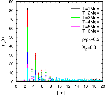
Figure 7: Proton pair correlation function for various temperatures, at a fixed density of $\rho/\rho_{{}_{0}}\!=\!0.2$, and a proton fraction of $x_{p}\!=\!0.3$.

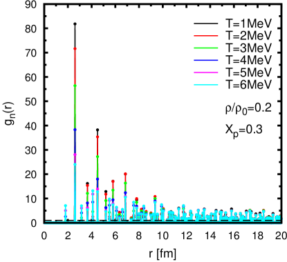
Figure 8: Neutron pair correlation function for various temperatures, at a fixed density of $\rho/\rho_{{}_{0}}\!=\!0.2$, and a proton fraction of $x_{p}\!=\!0.3$.

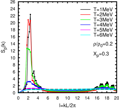
Figure 9: Proton static structure form factor for various temperatures, at a fixed density of $\rho\!/\!\rho_{{}_{0}}\!=\!0.2$, and a proton fraction of $x_{p}\!=\!0.3$.

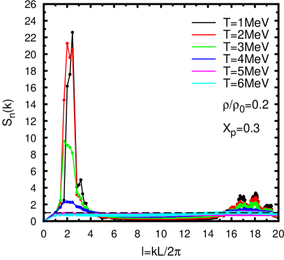
Figure 10: Neutron static structure form factor for various temperatures, at a fixed density of $\rho/\rho_{{}_{0}}\!=\!0.2$, and a proton fraction of $x_{p}\!=\!0.3$.

The $T\!=\!1\,{\rm MeV}$ results set the baseline as these can be directly compared against our earlier findings. As before, at low temperatures ($T\!\lesssim\!3\,{\rm MeV}$) the system displays the strong clustering correlations characteristic of the pasta phase. However, as the temperature increases and the thermal energy becomes comparable to the binding energy per nucleon of the neutron-rich clusters the behavior changes dramatically. The large peaks in both the pair correlation function and the static structure factor get significantly reduced as the system reaches a temperature of $T\!\simeq\!4\,{\rm MeV}$ and both become essentially structurless at $T\!\gtrsim\!5\,{\rm MeV}$. Note also the appearance of a small peak in $g_{n}(r)$ at $r\!=\!a$ as the entropic contribution starts to become as important, if not more, than the energy contribution.

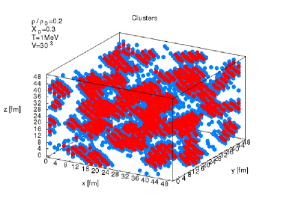
Figure 11: Monte-Carlo snapshot of neutron-star matter at a temperature of $T\!=\!1\,{\rm MeV}$, a density of $\rho/\rho_{{}_{0}}\!=\!0.2$, and a proton fraction of $x_{p}\!=\!0.3$. The blue and red dots are used to display the location of neutrons and protons, respectively.

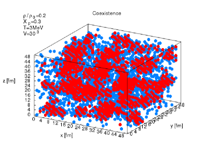
Figure 12: Monte-Carlo snapshot of neutron-star matter at a temperature of $T\!=\!3\,{\rm MeV}$, a density of $\rho/\rho_{{}_{0}}\!=\!0.2$, and a proton fraction of $x_{p}\!=\!0.3$. The blue and red dots are used to display the location of neutrons and protons, respectively.

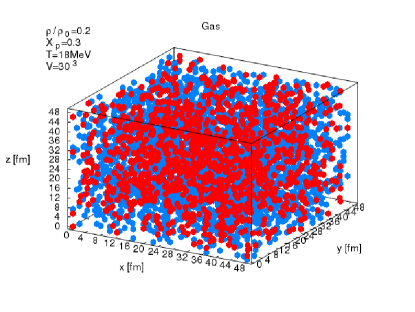
Figure 13: Monte-Carlo snapshot of neutron-star matter at a temperature of $T\!=\!18\,{\rm MeV}$, a density of $\rho/\rho_{{}_{0}}\!=\!0.2$, and a proton fraction of $x_{p}\!=\!0.3$. The blue and red dots are used to display the location of neutrons and protons, respectively.

To illustrate the behavior of the system as a function of temperature we display in Figs. 11-13 Monte-Carlo snapshots at a density of $\rho/\rho_{{}_{0}}\!=\!0.2$, a proton fraction of $x_{p}\!=\!0.3$, and temperatures of $T\!=\!1\,{\rm MeV}$, $T\!=\!3\,{\rm MeV}$, and $T\!=\!18\,{\rm MeV}$. One can see the gradual transition in the structure of the system. At $T\!=\!1\,{\rm MeV}$ the system displays the existence of neutron-rich clusters surrounded by a dilute neutron vapor. As the temperature is increased to $T\!=\!3\,{\rm MeV}$, some of the weakly bound neutrons in the clusters join the vapor and one sees a coexistence between the clusters and the vapor. Finally, at the very large temperature of $T\!=\!18\,{\rm MeV}$ no spatial correlations remain as the system has been fully vaporized into a classical gas of nucleons. Quantitatively, this behavior is captured by the heat capacity which has been computed by calculating the fluctuations in energy [see Eq. (16)] and is displayed in Fig. 14. The energy fluctuations are small in both the clustered and gas phases—but increases significantly at $T\!\simeq\!3\,{\rm MeV}$ where both phases coexists.

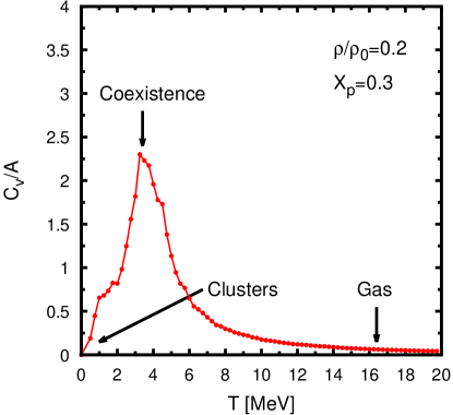
Figure 14: The heat capacity of neutron-star matter as a function of temperature and at a density of $\rho/\rho_{{}_{0}}\!=\!0.2$ and a proton fraction of $x_{p}\!=\!0.3$.

IV Conclusions and Outlook

The quest for physical observables that are particularly sensitive to pasta formation remains elusive. Indeed, even the existence of the pasta phase in the proton-deficient environment of the inner stellar crust remains an open question. In the present work we introduced a new model—the “Charged Ising Model”—to tackle some of these fundamental questions. The CIM is a lattice-gas model that while simple in its assumptions, retains the essence of Coulomb frustration that is required to capture the subtle dynamics of the inner stellar crust. Monte Carlo simulations based on this model are not as computationally demanding because the long-range Coulomb interaction—computed here exactly via an Ewald summation—was pre-computed at the appropriate lattice sites and then stored in memory prior to the start of the simulation. This represents an enormous advantage in simulating systems with a large number of particles as a function of density, temperature, and proton fraction. In this first—and mostly exploratory study—we were able to simulate systems with as many as $S\!=\!30^{3}$ lattice sites as a function of temperature, density, and proton fraction. Particular attention was placed on physical observables such as the pair correlation function, the corresponding static structure factor, and the heat capacity; quantities that properly capture both density and thermal fluctuations in the system. Note that the static structure factor displays a prominent coherent peak that occurs at a momentum transfer for which the probe (e.g., electrons in the case of protons and neutrinos in the case of neutrons) can most efficiently scatter from the density fluctuations in the system. The existence of pasta structures can therefore significantly reduce the electron or neutrino mean-free path in the stellar crust. A detailed study of electron and neutrino transport within the CIM will be forthcoming. We note that the very simple nuclear part of the Hamiltonian [Eqs. (2) and (3)] essentially represents an Ising Hamiltonian for a spin-one system. That is,

$$V_{\rm Nuclear}=\frac{\epsilon}{2}\sum_{\langle i,j\rangle}^{S}n_{i}n_{j}\,,$$ (23)

where $\epsilon\!\simeq\!16/3\,{\rm MeV}$ but now $n_{i}\!=\!-1,0,1$ can take three values depending on whether the site is occupied by a neutron, is empty, or is occupied by a proton. To properly simulate neutron-star matter, this Hamiltonian—together with the long-range Coulomb part—must be solved at constant magnetization rather than at constant magnetic field. Although much work has been done along the lines of the Ising model, the virtue of the CIM is that it incorporates the relatively simple spin-1 Ising model together with the challenging long-range Coulomb interactions.

Finally, in the future we plan to use the CIM to carry out an analysis similar to the one recently reported in Ref. Pramudya2011 . In such a condensed-matter study a large temperature gap, i.e., $k_{B}T_{c}\!<\!k_{B}T\!\ll\!E_{\rm Coul}$, was identified between the melting temperature and the Coulomb energy where the system displays unconventional “pasta-like” behavior as a result of the strong frustration induced by the long-range interactions. Particularly relevant is the emergence of a pseudogap in the density of states that appears to mediate the transition from the Wigner Crystal to the uniform Fermi liquid. We are confident that the evolution of the pseudogap region as a function of proton fraction may help us prove the existence—or lack-thereof—of a pasta phase in the inner stellar crust.

- (1) J. R. Oppenheimer and G. M. Volkoff, Phys. Rev. 55, 374 (1939).
- (2) I. Bombaci, A&A 305, 871 (1996).
- (3) N. K. Glendenning, Compact Stars: Nuclear Physics, Particle Physics, and General Relativity, Springer-Verlag (2000).
- (4) N. K. Glendenning, Phys. Rep. 342, 393 (2001).
- (5) The Committee on the Assessment of and Outlook for Nuclear Physics; Board on Physics and Astronomy; Division on Engineering and Physical Sciences; National Research Council, “Nuclear Physics: Exploring the Heart of Matter”, The National Academies Press (2012).
- (6) P. J. Ellis, R. Knorren, and M. Prakash, Phys. Lett. B 349, 11 (1995).
- (7) J. A. Pons, J. A. Miralles, M. Prakash, and J. M. Lattimer, Astrophys. J. 553, 382 (2001).
- (8) F. Weber, Prog. Part. Nucl. Phys. 54, 193 (2005).
- (9) M. G. Alford, K. Rajagopal, and F. Wilczek, Nucl. Phys. B 537, 443 (1999).
- (10) M. G. Alford, A. Schmitt, K. Rajagopal, and T. Schafer, Rev. Mod. Phys. 80, 1455 (2008).
- (11) C. J. Horowitz, M. A. Pérez-García, and J. Piekarewicz, Phys. Rev. C 69, 045804 (2004).
- (12) G. Watanabe, T. Maruyama, K. Sato, K. Yasuoka, and T. Ebisuzaki, Phys. Rev. Lett. 94, 031101 (2005).
- (13) Jérôme Margueron, Jesús Navarro, and Patrick Blottiau, Phys. Rev. C 70, 028801 (2004).
- (14) N. Chamel and P. Haensel, Living Rev. Relativity 11 (2008), 10.
- (15) C. Bertulani and J. Piekarewicz editors, “Neutron Star Crust”, Nova Publishers (2012).
- (16) D. G. Ravenhall, C. J. Pethick, and J. R. Wilson, Phys. Rev. Lett. 50, 2066 (1983).
- (17) C. P. Lorenz, D. G. Ravenhall, and C. J. Pethick, Phys. Rev. Lett. 70, 379 (1993).
- (18) D.G. Ravenhall and C.J. Pethick, Annu. Rev. Nucl. Part. Sci. 45 429 (1995).
- (19) C. J. Horowitz, M. A. Pérez-García, J. Carriere, D. K. Berry, and J. Piekarewicz, Phys. Rev. C 70, 065806 (2004).
- (20) C. J. Horowitz, M. A. Pérez-García, D. K. Berry, and J. Piekarewicz, Phys. Rev. C 72, 035801 (2005).
- (21) T. Maruyama, K. Niita, K. Oyamatsu, T. Maruyama, S. Chiba, and A. Iwamoto, Phys. Rev. C 57, 655 (1998).
- (22) G. Watanabe, K. Sato, K. Yasuoka, and T. Ebisuzaki, Phys. Rev. C 66, 012801 (2002).
- (23) G. Watanabe, K. Sato, K. Yasuoka, and T. Ebisuzaki, Phys. Rev. C 68, 035806 (2003).
- (24) G. Watanabe, K. Sato, K. Yasuoka, and T. Ebisuzaki, Phys. Rev. C 69, 055805 (2004).
- (25) H. Sonoda, G. Watanabe, K. Sato, T. Takiwaki, K. Yasuoka, and T. Ebisuzaki, Phys. Rev. C 75, 042801 (2007).
- (26) H. Sonoda, G. Watanabe, K. Sato, K. Yasuoka, and T. Ebisuzaki, Phys. Rev. C 77, 035806 (2008).
- (27) G. Watanabe, H. Sonoda, T. Maruyama, K. Sato, K. Yasuoka, and T. Ebisuzaki, Phys. Rev. Lett. 103, 121101 (2009).
- (28) G. Watanabe, K. Sato, K. Yasuoka, and T. Ebisuzaki, Phys. Rev. C 81, 049901 (2010).
- (29) H. Sonoda, G. Watanabe, K. Sato, K. Yasuoka, and T. Ebisuzaki, Phys. Rev. C 81, 049902 (2010).
- (30) B. Jouault, F. Sébille, and V. de la Mota, Nucl. Phy. A628, 119 (1998).
- (31) F. Sébille, V. de la Mota, and S. Figerou, Nucl. Phy. A822, 51 (2009).
- (32) F. Sébille, V. de la Mota, and S. Figerou, Phys. Rev. C 84, 055801 (2011).
- (33) T. Maruyama, T. Tatsumi, D. N. Voskresensky, T. Tanigawa, and S. Chiba Phys. Rev. C 72, 015802 (2005).
- (34) T. Maruyama, T. Tatsumi, D. N. Voskresensky, T. Tanigawa, T. Endo, and S. Chiba Phys. Rev. C 73, 035802 (2006).
- (35) S. S. Avancini, D. P. Menezes, M. D. Alloy, J. R. Marinelli, M. M. W. Moraes, and C. Providência, Phys. Rev. C 78, 015802 (2008).
- (36) S. S. Avancini, L. Brito, J. R. Marinelli, D. P. Menezes, M. M. W. de Moraes, C. Providência, and A. M. Santos Phys. Rev. C 79, 035804 (2009).
- (37) F. Grill, C. Providência, and S. S. Avancini, Phys. Rev. C 85, 055808 (2012).
- (38) W. G. Newton and J. R. Stone, Phys. Rev. C 79, 055801 (2009).
- (39) J. Piekarewicz and G. Toledo Sánchez, Phys. Rev. C 85, 015807 (2012).
- (40) Y. Pramudya, H. Terletska, S. Pankov, E. Manousakis, and V. Dobrosavljević, Phys. Rev. B 84, 125120 (2011).
- (41) P. Napolitani, Ph. Chomaz, F. Gulminelli, and K. H. O. Hasnaoui, Phys. Rev. Lett. 98, 131102 (2007).
- (42) C. Ducoin, K. H. O. Hasnaoui, P. Napolitani, Ph. Chomaz, and F. Gulminelli, Phys. Rev. C 75, 065805 (2007).
- (43) Ph. Chomaz, C. Ducoin, F. Gulminelli, K. Hasnaoui, and P. Napolitan, Nucl. Phy. A787, 603 (2007).
- (44) P. P. Ewald, Ann. Phys. 369, 253 (1921).
- (45) M. P. Allen, D. J . Tildesley, Computer Simulation of liquids, Clarendon, London (1987).
- (46) A. Y. Abdulnour and J.A. Board Jr, Computer Physics Communications 95 73 (1996).
- (47) N. Metropolis, A. W. Rosenbluth, M. N. Rosenbluth, A. H. Teller, and E. Teller, J. Chem. Phys. 21, 1087 (1953).
- (48) A. L. Fetter and J. D. Walecka, Quantum Theory of Many Particle Systems, McGraw-Hill, New York (1971).
- (49) F. J. Vesely, Computational Physics: An Introduction, Kluwer Academic, New York (2001).
- (50) R. K. Pathria, Statistical Mechanics, Butterworth-Heinemann, Oxford (1996).