Transitions in rapidly rotating convection driven dynamos

Abstract

Numerical simulations of dynamos in rotating Rayleigh-Bénard convection in plane layers are presented. Two different types of dynamos exist which obey different scaling laws for the amplitude of the magnetic field. The transition between the two occurs within a hydrodynamically uniform regime which can be classified as rapidly rotating convection.

Most celestial bodies are the seat of a magnetic field. It is commonly assumed that this field is either a fossil field remaining from the formation process of the body, or that it is maintained by the dynamo effect which converts kinetic energy of the motion of a liquid or gaseous electric conductor into magnetic energy. It is in many cases reasonable to suppose that the motion of the fluid conductor is driven by convection. The minimal model of a convection driven dynamo is a horizontal plane layer in a gravity field, filled with electrically conducting fluid, heated from below and cooled from above, and rotating about a vertical axis. Such a plane layer may be viewed as a local approximation to the astrophysically more relevant spherical geometry.

Several studies of this problem exist and they have found different types of magnetic fields Jones and Roberts (2000); Rotvig and Jones (2002); Stellmach and Hansen (2004); Cattaneo and Hughes (2006). Depending on whether rapidly or slowly rotating layers are simulated, the magnetic fields are either generated at the largest available spatial scale or at smaller scales. The generated magnetic fields contain either a large or small mean field (where the mean is obtained by averaging over horizontal planes), and the magnetic field in the final statistically stationary state either executes small fluctuations around a well defined mean or experiences large swings during which the field amplitude varies by an order of magnitude and more.

This paper presents simulations of dynamos in rotating and convecting plane layers. If the convection is driven stronger and stronger at fixed rotation rate, the flow behaves at some point as if it was not rotating. This transition shows in the scaling of the heat transport which can be used to distinguish slow from rapid rotation Schmitz and Tilgner (2009); King et al. (2009). Within the convection flows which are rapidly rotating according to this criterion, it will be shown below that different types of dynamos exist.

Consider a plane layer with boundaries perpendicular to the $z-$axis, rotating about this axis with angular velocity $\bm{\Omega}=\Omega\hat{\bm{z}}$, where the hat denotes a unit vector. Gravity $\bm{g}$ is pointing along the negative $z-$direction, $\bm{g}=-g\hat{\bm{z}}$. The layer is filled with electrically conducting fluid of density $\rho$, kinematic viscosity $\nu$, thermal diffusivity $\kappa$, thermal expansion coefficient $\alpha$, and magnetic diffusivity $\lambda$. The fluid is moving according to the velocity field $\bm{v}(\bm{r},t)$ which depends on position $\bm{r}$ and time $t$. The fluid is also permeated by the magnetic field $\bm{B}(\bm{r},t)$ and has temperature $T(\bm{r},t)$.

The boundaries are located in the planes $z=0$ and $z=d$. These boundaries are assumed to be at constant temperatures $T_{0}+\Delta T$ and $T_{0}$, respectively. The boundaries are also assumed to be free slip and the space outside the fluid layer is assumed to be a perfect conductor. The boundary conditions therefore read $T=T_{0}+\Delta T$ at $z=0$, $T=T_{0}$ at $z=d$, and furthermore $v_{z}=\partial_{z}v_{y}=\partial_{z}v_{x}=B_{z}=\partial_{z}B_{y}=\partial_{z}B_{x}=0$ at $z=0$ and $d$. Periodic boundary conditions are imposed in the lateral directions forcing all fields to have periodicity lengths $l_{x}$ and $l_{y}$ in the $x-$ and $y-$directions.

The equations have been solved numerically in the nondimensional form which obtains if one uses $d$, $d^{2}/\kappa$, $\kappa/d$, $\rho\kappa^{2}/d^{2}$, $\Delta T$ and $\sqrt{\mu_{0}\rho}\kappa/d$ as units of length, time, velocity, pressure, temperature difference from $T_{0}$, and magnetic field, respectively. Four control parameters appear in the equations: The Rayleigh number $\mathrm{Ra}$, the Ekman number $\mathrm{Ek}$, the Prandtl number $\mathrm{Pr}$, and the magnetic Prandtl number $\mathrm{Pm}$. They are defined by

$$\mathrm{Ra}=\frac{g\alpha\Delta Td^{3}}{\kappa\nu}~{}~{}~{},~{}~{}~{}\mathrm{Ek}=\frac{\nu}{\Omega d^{2}}~{}~{}~{},~{}~{}~{}\mathrm{Pr}=\frac{\nu}{\kappa}~{}~{}~{},~{}~{}~{}\mathrm{Pm}=\frac{\nu}{\lambda}$$ (1)

The nondimensional equations read (using the same variables for the nondimensional quantities as their dimensional counter parts):

$$\partial_{t}\rho+\nabla\cdot\bm{v}=0$$ (2)

$$\begin{split}\partial_{t}\bm{v}+(\bm{v}\cdot\nabla)\bm{v}+2\frac{\mathrm{Pr}}{\mathrm{Ek}}\hat{\bm{z}}\times\bm{v}=\\ -c^{2}\nabla\rho+\mathrm{Pr}~{}\mathrm{Ra}~{}\theta\hat{\bm{z}}+\mathrm{Pr}\nabla^{2}\bm{v}+(\nabla\times\bm{B})\times\bm{B}\end{split}$$ (3)

$$\partial_{t}\theta+\bm{v}\cdot\nabla\theta-v_{z}=\nabla^{2}\theta$$ (4)

$$\partial_{t}\bm{B}+\nabla\times(\bm{B}\times\bm{v})=\frac{\mathrm{Pr}}{\mathrm{Pm}}\nabla^{2}\bm{B}$$ (5)

$$\nabla\cdot\bm{B}=0$$ (6)

where $\theta$ is the deviation from the conductive temperature profile so that $\theta=0$ at the top and bottom boundaries. From now on, only nondimensional variables will be used.

The above equations approximate the Boussinesq equations using the method of artificial compressibility Chorin (1967), which assumes an equation of state of the form $p=c^{2}\rho$, where $p$ stands for the pressure and $c$ for the velocity of sound. If one develops the variables $p$, $\bm{v}$, $\theta$ and $\bm{B}$ in powers of $1/c^{2}$ (as for example in $\theta=\theta_{0}+\frac{1}{c^{2}}\theta_{1}+\frac{1}{c^{4}}\theta_{2}+...$) and inserts these series into equations (2-6) together with $p=c^{2}\rho$, one recovers the Boussinesq equations at the order $(1/c^{2})^{0}$. This method simulates the standard Boussinesq equations if the Mach number is small and if the time it takes sound to travel across the layer is much less than the rotation period, i.e. if $c^{2}\gg(1/2\pi)^{2}(\mathrm{Pr}/\mathrm{Ek})^{2}$. In all the simulations reported here, the Mach number was less than 0.1 and $c^{2}\mathrm{Ek}^{2}>0.4$. The validity of the entire approach was tested by reproducing a few results of ref. Stellmach and Hansen (2004); Schmitz and Tilgner (2009) in which the Boussinesq equations are solved. The numerical simulations used a finite difference method implemented on GPUs. The method is the same as the one in ref. Tanriverdi and Tilgner (2011); *Tilgne11 except that fourth order spatial derivatives have been used in the induction and all diffusion terms. Spatial resolutions have been adapted to the control parameters and went up to $256^{3}$. The runs were divided into six series, three for $\mathrm{Pm}=1$ and the other three for $\mathrm{Pm}=3$, while $\mathrm{Pr}$ was always set to $0.7$. For each $\mathrm{Pm}$, the Ekman numbers $2\times 10^{-4}$, $2\times 10^{-5}$, and $2\times 10^{-6}$ have been used. Within each of the six series, $\mathrm{Ra}$ was varied from its critical value up to 100 times critical for $\mathrm{Ek}=2\times 10^{-4}$ and three times critical for $\mathrm{Ek}=2\times 10^{-6}$. Because the typical length scale of convection varies with $\mathrm{Ek}$, the periodicity lengths were set to $l_{x}/d=l_{y}/d=1$, $1/2$, and $1/4$ for $\mathrm{Ek}=2\times 10^{-4}$, $2\times 10^{-5}$ and $2\times 10^{-6}$, respectively. All runs have been started from magnetic seed fields small enough so that the seed field does not modify the convection and cannot lead to subcritical bifurcation.

The output of the computations include the densities of kinetic and magnetic energies, $e_{\mathrm{kin}}$ and $e_{B}$, defined by

$$e_{\mathrm{kin}}=\frac{1}{V}\int\frac{1}{2}\bm{v}^{2}dV~{}~{}~{},~{}~{}~{}e_{B}=\frac{1}{V}\int\frac{1}{2}\bm{B}^{2}dV,$$ (7)

where the integration extends over the entire fluid volume $V$. If we denote the time average by angular brackets, one can compute average energy densities $E_{\mathrm{kin}}$ and $E_{B}$ from $E_{\mathrm{kin}}=\langle e_{\mathrm{kin}}\rangle$ and $E_{B}=\langle e_{B}\rangle$ as well as the Reynolds number $\mathrm{Re}$ from $\mathrm{Re}=\langle\sqrt{2e_{\mathrm{kin}}}\rangle/\mathrm{Pr}$. The magnetic Reynolds number $\mathrm{Rm}$ is defined as $\mathrm{Rm}=\mathrm{Re}\,\mathrm{Pm}$.

When the Rayleigh number is increased within each series of computations at constant $\mathrm{Ek}$ and $\mathrm{Pm}$, one finds an onset of dynamo action, and in most series an interval of $\mathrm{Ra}$ in which self-sustained magnetic fields do not exist before dynamo action starts anew at higher $\mathrm{Ra}$. A preliminary set of computations solved the kinematic dynamo problem, in which the back reaction of the magnetic field on the flow is neglected. For this purpose, the $(\nabla\times\bm{B})\times\bm{B}$ term was removed form eq. (3) and the remaining system of partial differential equations integrated in time. Without the $(\nabla\times\bm{B})\times\bm{B}$ term, initial magnetic seed fields either grow or decay indefinitely after transients have passed. They do so in a fluctuating manner if the flow is chaotic, but viewed on long time scales, the magnetic energy grows or decays exponentially as $e^{pt}$. The growth rate $p$ is shown as a function of $\mathrm{Rm}\,\mathrm{Ek}^{1/3}$ in fig. 1. In this representation, the local minimum of $p$ is found at the same position for all $\mathrm{Ek}$ and $\mathrm{Pm}$ near $\mathrm{Rm}\,\mathrm{Ek}^{1/3}=13.5$. Choosing $\mathrm{Rm}\,\mathrm{Ek}^{1/3}$ as parameter does not lead to an overlap of all data in fig. 1. For instance, the local maximum of $p$ at $\mathrm{Rm}\,\mathrm{Ek}^{1/3}<13.5$ occurs at various values of $\mathrm{Rm}\,\mathrm{Ek}^{1/3}$ and analytical work tells us that the dynamo onset (which was not accurately located in the present simulations) occurs at $\mathrm{Rm}\,\mathrm{Ek}^{1/6}=const.$ Soward (1974). The product $\mathrm{Rm}\,\mathrm{Ek}^{1/3}$ is proportional to the magnetic Reynolds number on the length scale of one column in the convective flow, because in the limit of small $\mathrm{Ek}$, the wavelength of the flow at the onset of convection is given by $3.83\cdot\mathrm{Ek}^{1/3}$. At the local minimum, $p$ is negative in all cases except for $\mathrm{Ek}=2\times 10^{-6}$, $\mathrm{Pm}=3$. Since $\mathrm{Rm}$ increases monotonically with $\mathrm{Ra}$ (see fig. 2 below), this means that a stronger driving does not necessarily help the dynamo.

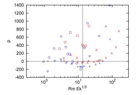
Figure 1: (Color online) Growth rate $p$ of magnetic energy in kinematic dynamo calculations as a function of $\mathrm{Rm}\,\mathrm{Ek}^{1/3}$. Results for $Pm=1$ are shown in blue and those for $Pm=3$ are in red. For $Pm=1$, the Ekman numbers of $2\times 10^{-4}$, $2\times 10^{-5}$, and $2\times 10^{-6}$ are indicated by the plus sign, triangle down, and circle, respectively, whereas for $Pm=3$, the same Ekman numbers are indicated by the x sign, triangle up, and square. The vertical line is located at $\mathrm{Rm}\,\mathrm{Ek}^{1/3}=13.5$.

This conclusion is also valid for no slip boundary conditions. Ekman layers appear at no slip boundaries which induce vertical flow in the bulk and potentially help the dynamo effect by increasing helicity. However, the same sequence of positive and negative growth rates shown in fig. 1 was also found for no slip boundaries by varying $\mathrm{Ra}$ for $\mathrm{Ek}=2\times 10^{-4}$, $\mathrm{Pm}=3$.

From now on, all results are for the full set of equations (2-6) including the $(\nabla\times\bm{B})\times\bm{B}$ term. A global view of all simulations is presented in fig. 2. The successful and failed dynamos are shown in the plane spanned by $\mathrm{Rm}\,\mathrm{Ek}^{1/3}$, the parameter already used in fig. 1, and $\mathrm{Re}\,\mathrm{Pr}\,\mathrm{Ek}^{1/2}$. This parameter was introduced in Schmitz and Tilgner (2009, 2010) because in nonmagnetic convection, the nondimensional heat flux, expressed as the Nusselt number $\mathrm{Nu}$ and combined with $\mathrm{Ek}$ into the quantity $\mathrm{Nu}\,\mathrm{Ek}^{1/3}$, obeys simple scaling laws in the two limits of $\mathrm{Re}\,\mathrm{Pr}\,\mathrm{Ek}^{1/2}$ small (corresponding to flows dominated by rotation) and large (approaching the limit of nonrotating flows). The two asymptotes fitting the two limits cross at $\mathrm{Re}\,\mathrm{Pr}\,\mathrm{Ek}^{1/2}=2$, which therefore separates the flows dominated by the Coriolis force from those who behave the same as nonrotating flows in as far as the scaling of the heat flux is concerned. (It remains to be investigated how this criterion relates to changes in flow structures or statistics of velocity fluctuations Stevens et al. (2010); *Kunnen06.) It is seen in fig. 2 that the transition line at $\mathrm{Rm}\,\mathrm{Ek}^{1/3}=13.5$ identified in fig. 1 is crossed at $\mathrm{Re}\,\mathrm{Pr}\,\mathrm{Ek}^{1/2}<2$ by all series except the one for $\mathrm{Ek}=2\times 10^{-4}$, $\mathrm{Pm}=1$.

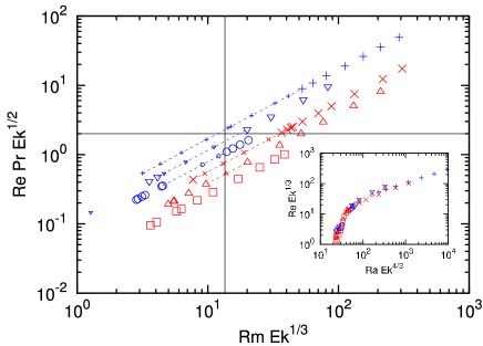
Figure 2: (Color online) Successful dynamos are shown with large and failed dynamos with small symbols (located on a broken line in the window without dynamo action) in the plane spanned by $\mathrm{Rm}\,\mathrm{Ek}^{1/3}$ and $\mathrm{Re}\,\mathrm{Pr}\,\mathrm{Ek}^{1/2}$. The meaning of the symbol shapes is the same as in fig. 1 and the lines indicate $\mathrm{Rm}\,\mathrm{Ek}^{1/3}=13.5$ and $\mathrm{Re}\,\mathrm{Pr}\,\mathrm{Ek}^{1/2}=2$. The inset shows $\mathrm{Re}\,\mathrm{Ek}^{1/3}$ (which is proportional to the Reynolds number based on the size of the convection columns) as a function of $\mathrm{Ra}\,\mathrm{Ek}^{4/3}$ (which is proportional to the ratio of $\mathrm{Ra}$ to the critical Rayleigh number for the onset of convection) for the same simulations.

It will now be argued that the dynamos both below and above the transition are related to dynamos known from previous work. Below the transition, the dynamos qualify as $\alpha^{2}-$dynamos in the language of mean-field magnetohydrodynamics and rely on the helicity of the flow Stellmach and Hansen (2004). The classification of the dynamos above the transition is more difficult. Cattaneo and Hughes Cattaneo and Hughes (2006) found convection driven dynamos which present the characteristics expected from dynamos in a chaotic flow with little or no helicity. These dynamos generate magnetic fields at small length scales and with little mean field. The distinction between generation at large and small scales is pointless for the flows studied here because all flows look similar to those visualized in ref. Stellmach and Hansen (2004): They consist of long thin vortices aligned with the rotation axis with little interior structure, so that in horizontal planes, large and small scales are identical. The energy contained in the mean magnetic field is less than 30 % of the total magnetic energy in all cases simulated here and this ratio smoothly decreases with increasing magnetic Reynolds number. At $\mathrm{Rm}\,\mathrm{Ek}^{1/3}=13.5$, this ratio is down to 7 %, so that these features are not useful for identifying the generation mechanism.

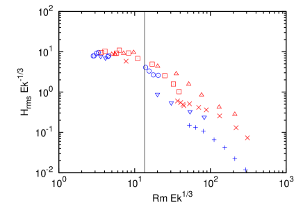
Figure 3: (Color online) $H_{\mathrm{rms}}\mathrm{Ek}^{-1/3}$ as a function of $\mathrm{Rm}\,\mathrm{Ek}^{1/3}$ for the successful dynamos of fig. 2. The vertical line is located at $\mathrm{Rm}\,\mathrm{Ek}^{1/3}=13.5$.

A more important hint is provided by helicity. Following refs. Cattaneo and Hughes (2006); Schmitz and Tilgner (2010), we define as helicity $\langle H\rangle$ the correlation $\bm{v}\cdot\nabla\times\bm{v}/(|\bm{v}|\cdot|\nabla\times\bm{v}|)$ between velocity and vorticity averaged over horizontal planes and time, which still depends on $z$. We obtain a single number $H_{\mathrm{rms}}$ as measure of helicity from $H_{\mathrm{rms}}=\int_{0}^{1}\langle H\rangle^{2}dz$. As fig. 3 shows, $H_{\mathrm{rms}}\mathrm{Ek}^{-1/3}$ is nearly constant below the transition and decreases above. The helicity is apparently held constant by the magnetic field below the transition, because in nonmagnetic convection, helicity continuously decreases with increasing Reynolds number Schmitz and Tilgner (2010). The decrease of helicity above the transition does not prevent magnetic fields from growing, which shows that helicity is not required for dynamo action above the transition. We therefore arrive at a picture in which there are two mechanisms responsible for dynamo action. One is based on helicity and dominates below the transition, but it becomes less and less efficient at high magnetic Reynolds numbers. The other is independent of helicity and takes over at high magnetic Reynolds numbers. Field amplification by chaotic stretching is intrinsically a mechanism requiring high magnetic Reynolds numbers, which fits well with the fact that the transition occurs at a certain value of $\mathrm{Rm}\,\mathrm{Ek}^{1/3}$.

Another type of transition is known from convection dynamos in spheres, where the field can transit from a field dominated by its dipole contribution to a field with a much smaller dipole moment. This transition occurs at a Rossby number based on the size of the vortices in the flow of about 0.1 Christensen and Aubert (2006), which in the present notation corresponds to $(\mathrm{Re}\,\mathrm{Ek})\mathrm{Ek}^{1/3}=0.052$. Nothing indicates a transition as a function of this Rossby number in the present simulations. More recent simulations in spherical shells Soderlund et al. (2012), however, find the transition when inertial and viscous forces become comparable.

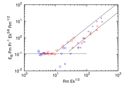
Figure 4: (Color online) $E_{B}\,\mathrm{Ek}^{5/6}\,\mathrm{Pm}/(\mathrm{Rm}^{1/2}\,\mathrm{Pr})$ as a function of $\mathrm{Rm}\,\mathrm{Ek}^{1/3}$ with the same symbols as in fig. 1. The horizontal line marks the value of 0.11, and the other lines show $(\mathrm{Rm}\,\mathrm{Ek}^{1/3})^{3/2}$.

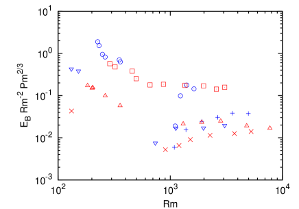
Figure 5: (Color online) Same data as in fig. 4 but plotted as $E_{B}\,\mathrm{Rm}^{-2}\,\mathrm{Pm}^{2/3}$ versus $\mathrm{Rm}$. Only the successful dynamos appear in figs. 4 and 5 since $E_{B}=0$ for the others.

The scaling of the amplitude of the generated magnetic field in the statistically stationary state depends on whether the dynamo is below or above the transition. Below the transition, the magnetic field strength obeys a scaling indicative of a magnetostrophic balance, in which the Lorentz force is in equilibrium with the Coriolis force. Some fraction of the Coriolis and Lorentz forces is balanced by the pressure gradient, but it is impossible to compute that fraction from the data actually saved during the simulations. We will equate naive estimates for both forces, replacing the Coriolis and Lorentz terms in eq. (3) by $\mathrm{Re}\,\mathrm{Pr}/\mathrm{Ek}$ and $E_{B}/l_{B}$, respectively, where $l_{B}$ stands for the length scale on which the magnetic field typically varies. From simulations of pure convection Schmitz and Tilgner (2009) we know that the size of the convection columns stays close to the size they have at the onset of convection throughout the parameter range of interest here, i.e. close to $1.9\cdot\mathrm{Ek}^{1/3}$. The magnetic Reynolds number based on that size varies for the dynamos below the transition from 4.8 to 25. At these Reynolds numbers, the magnetic field is not distributed uniformly but is expelled from the core of the vortices and concentrates in boundary layers of thickness proportional to $\mathrm{Ek}^{1/3}(\mathrm{Rm}\,\mathrm{Ek}^{1/3})^{-1/2}$. Using this expression for $l_{B}$, the assumption of magnetostrophic balance leads to $E_{B}\,\mathrm{Ek}^{5/6}\,\mathrm{Pm}/(\mathrm{Rm}^{1/2}\,\mathrm{Pr})=const.$. It is verified in fig. 4 that the left hand side of this equation is $0.11\pm 0.03$ for all dynamos below the transition, the largest deviations being due to the simulations at low $\mathrm{Ek}$ with widely fluctuating energies typical for this parameter range Stellmach and Hansen (2004) and which require long runs before accurate values of $E_{B}$ and $\mathrm{Rm}$ are obtained.

As suggested by fig. 5 and the asymptotes drawn into fig. 4, the magnetic field obeys a scaling close to $E_{B}\propto\mathrm{Rm}^{2}$ above the transition. Such a behavior arises if there is equipartition between kinetic and magnetic energies, or if there is a balance between advection and Lorentz terms and if the same length scale is used to estimate these two terms in eq. (3). None of this is apparently exactly realized in the present simulations because a nontrivial dependence on $\mathrm{Ek}$ and $\mathrm{Pm}$ remains.