A Note on the Deletion Channel Capacity

Abstract

Memoryless channels with deletion errors as defined by a stochastic channel matrix allowing for bit drop outs are considered in which transmitted bits are either independently deleted with probability $d$ or unchanged with probability $1-d$. Such channels are information stable, hence their Shannon capacity exists. However, computation of the channel capacity is formidable, and only some upper and lower bounds on the capacity exist. In this paper, we first show a simple result that the parallel concatenation of two different independent deletion channels with deletion probabilities $d_{1}$ and $d_{2}$, in which every input bit is either transmitted over the first channel with probability of $\lambda$ or over the second one with probability of $1-\lambda$, is nothing but another deletion channel with deletion probability of $d=\lambda d_{1}+(1-\lambda)d_{2}$. We then provide an upper bound on the concatenated deletion channel capacity $C(d)$ in terms of the weighted average of $C(d_{1})$, $C(d_{2})$ and the parameters of the three channels. An interesting consequence of this bound is that $C(\lambda d_{1}+(1-\lambda))\leq\lambda C(d_{1})$ which enables us to provide an improved upper bound on the capacity of the i.i.d. deletion channels, i.e., $C(d)\leq 0.4143(1-d)$ for $d\geq 0.65$. This generalizes the asymptotic result by Dalai [1] as it remains valid for all $d\geq 0.65$. Using the same approach we are also able to improve upon existing upper bounds on the capacity of the deletion/substitution channel.

I Introduction

Channels with synchronization errors can be well modeled using bit drop outs and/or bit insertions as well as random errors. There are many different models adopted in the literature to describe these errors. Among them, a relatively general model is employed by Dobrushin [2] where memoryless channels with synchronization errors are described by a channel matrix allowing for the channel outputs to be of different lengths for different uses of the channel. As proved in the same paper, for such channels, information stability holds and Shannon capacity exists. However, the determination of the capacity remains elusive as the mutual information term to be maximized does not admit a single letter or finite letter form.

In the existing literature, several specific instances of this model are more widely studied. For instance, by a proper selection of the stochastic channel transition matrix, one obtains the i.i.d. deletion channel which represents one of the simplest models allowing for bit drop-outs which is the model considered in this paper. In a binary i.i.d. deletion channel, the transmitted bits are either received correctly and in the right order or deleted from the transmitted sequence altogether with a certain probability $d$ independent of each other. Neither the receiver nor the transmitter knows the positions of the deleted bits. Despite the simplicity of the model, the capacity for this channel is still unknown, and only a few upper and lower bounds are available [3, 4, 5, 6]. Other special cases of the general model by Dobrushin are the Gallager model allowing for insertions, deletions and substitution errors in which every transmitted bit is either deleted with probability of $d$, replaced with two random bits with probability of $i$, flipped with probability of $f$ or received correctly with probability of $1-d-i-f$. Substituting $i=0$ in the Gallager model results into the deletion/substitution channel model which is also considered in this paper. Another look at the deletion/substitution channel can be as a series concatenation of two independent channels such that the first one is a deletion only channel with deletion probability of $d$ and the second one is binary symmetric channel (BSC) with cross error probability of $s=\frac{f}{1-d}$. There are also some capacity upper and lower bounds for the Gallager’s deletion channel model in the literature, e.g.,  [7, 8, 9].

In this paper, we prove that the capacity of an i.i.d. deletion channel with deletion probability of $d$ as an arithmetic mean of two different deletion probabilities $d_{1}$ and $d_{2}$, i.e., $d=\lambda d_{1}+(1-\lambda)d_{2}$ for $\lambda\in[0,1]$, can be upper bounded in terms of the capacity and the parameters of the two newly considered deletion channels. The proof relies on the simple observation that the deletion channel with deletion probability $d$ can be considered as the parallel concatenation of two independent deletion channels with deletion probabilities $d_{1}$ and $d_{2}$ where each bit is either transmitted over the first channel with probability $\lambda$ or the second channel with probability $1-\lambda$.

Thanks to the presented inequality relation among the deletion channels capacity, we are able to improve upon the existing upper bounds on the capacity of the deletion channel for $d\geq 0.65$ [6]. The improvement is the result of the fact that the currently known best upper bounds are not convex for some range of deletion probabilities. More precisely, our result allows us to convexify the existing deletion channel capacity upper bound for $d\geq 0.65$, leading to a significant improvement of the upper bound. In other words, we are able to prove that for $0\leq\lambda\leq 1$, $C(\lambda d+1-\lambda)\leq\lambda C(d)$, resulting in $C(d)\leq 0.4143(1-d)$ for $d\geq 0.65$ which is tighter than the result in [6]. The same result for the asymptotic scenario $d\rightarrow 1$ was also obtained in [1] using a different approach; however our result is valid for $d\geq 0.65$ hence more general. We also note that the best known limiting lower bound (as $d\rightarrow 1$) is $0.1185(1-d)$ [3]. We also demonstrate that a similar improvement is possible for the case of deletion/substitution channels. As an example, we can prove that for $s=0.03$, an improved capacity upper bound is obtained for $d\geq 0.6$ over the best existing result given in [7].

The paper is organized as follows. In Section II, we prove the main result of the paper which relates the capacity of the three different deletion channels through an inequality. In Section III, we generalize the result to the case of deletion/substitution channels and the parallel concatenation of more than two channels. In Section IV, we present tighter upper bounds on the capacity of the deletion and deletion/substitution channels based on previously known best upper bounds, and comment on the limit of the capacity as the deletion probability approaches unity. We conclude the paper in Section V.

II Main Theorem

In this section, we provide the main result of the paper on the capacity of the deletion channel and its proof. Furthermore, we present a simple proof for the special case with $d_{2}=0$, i.e., $C(\lambda d_{1}+1-\lambda)\leq\lambda C(d_{1})$.

The theorem below states our basic result whose proof hinges on a simple observation.

Theorem 1.

Let $C(d)$ denotes the capacity of the i.i.d. deletion channel with deletion probability $d$, $\lambda\in[0,1]$ and $d=\lambda d_{1}+(1-\lambda)d_{2}$, then we have

$$C(d) \leq \lambda C(d_{1})+(1-\lambda)C(d_{2})+(1-d)\log(1-d)$$ (1)

$$-\lambda(1-d_{1})\log(\lambda(1-d_{1}))-(1-\lambda)(1-d_{2})\log((1-\lambda)(1-d_{2})).$$

Proof.

Let us consider two different deletion channels, ${\cal{C}}_{1}$ and ${\cal{C}}_{2}$, with deletion probabilities $d_{1}$ and $d_{2}$, input sequences of bits $\mbox{\boldmath$X$}_{1}$ and $\mbox{\boldmath$X$}_{2}$, and output sequences of bits $\mbox{\boldmath$Y$}_{1}$ and $\mbox{\boldmath$Y$}_{2}$, respectively. Denote their Shannon capacities by $C(d_{1})$ and $C(d_{2})$, respectively. Given a specific $\lambda\in(0,1)$, define a new binary input channel $\cal{C^{\prime}}$ (shown in Fig. 1) with input sequence of bits $X$ and output sequence of bits $Y$ as follows: each channel input symbol is transmitted through ${\cal{C}}_{1}$ with probability $\lambda$, and through ${\cal{C}}_{2}$ with probability $1-\lambda$, independently of each other. Neither the transmitter nor the receiver knows the specific realization of the “individual channel selection events,” i.e., they do not know which specific subchannel a symbol is transmitted through, and which specific subchannel each output symbol is received from. The following two lemmas demonstrate that 1) the new channel is a new i.i.d. deletion channel with deletion probability $d=\lambda d_{1}+(1-\lambda)d_{2}$, 2) if appropriate side information be provided for the transmitter and the receiver then the capacity of the genie-aided channel is upper bounded by

$$\lambda C(d_{1})+(1-\lambda)C(d_{2})+(1-d)\log(1-d)-\lambda(1-d_{1})\log(\lambda(1-d_{1}))-(1-\lambda)(1-d_{2})\log((1-\lambda)(1-d_{2})).$$

Combining these two results, the proof of the theorem follows easily by noting that the capacity of the new channel $\cal{C^{\prime}}$ cannot decrease with side information. ∎

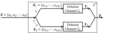
Figure 1: Channel Model $\cal{C^{\prime}}$

The following two lemmas are employed in the proof of the theorem.

Lemma 1.

$\cal{C^{\prime}}$ as defined in the proof of the theorem above is nothing but a deletion channel with deletion probability $d=\lambda d_{1}+(1-\lambda)d_{2}$.

Proof.

For each use of the channel $\cal{C^{\prime}}$, for any input symbol $x\in\cal{X}$ and channel output $y\in\cal{Y}$, the transition probability is given by $P\{{\cal{C}}_{1}\mbox{ is used}\}d_{1}+P\{{\cal{C}}_{2}\mbox{ is used}\}d_{2}=\lambda d_{1}+(1-\lambda)d_{2}$. Noting that the subchannels are memoryless and the channel selection events are independent of each other, this transition matrix precisely defines a deletion channel with deletion probability $d=\lambda d_{1}+(1-\lambda)d_{2}$. ∎

Lemma 2.

The capacity of the channel $\cal{C^{\prime}}$ as defined in the proof of the theorem above is upper bounded by

$$\lambda C(d_{1})+(1-\lambda)C(d_{2})+(1-d)\log(1-d)-\lambda(1-d_{1})\log(\lambda(1-d_{1}))-(1-\lambda)(1-d_{2})\log((1-\lambda)(1-d_{2})).$$

Proof.

We first define a new genie-aided channel which is obtained by providing the transmitter and the receiver of the channel $\cal{C^{\prime}}$ with appropriate side information, then derive an upper bound on the capacity of the genie-aided channel which is also an upper bound on the capacity of the channel $\cal{C^{\prime}}$. More precisely, we provide the transmitter with side information on which channel is being used for each transmitted symbol ($\mbox{\boldmath$X$}=\mbox{\boldmath$X$}_{1}\mbox{\boldmath$X$}_{2}$), and the receiver with side information on which channel the received symbol comes from ($\mbox{\boldmath$Y$}=\mbox{\boldmath$Y$}_{1}\mbox{\boldmath$Y$}_{2}$), and reveal the side information on the fragmentation information, i.e., random process $\mbox{\boldmath$F$}_{y}$, to the receiver such that by knowing $\mbox{\boldmath$F$}_{y}$, $\mbox{\boldmath$Y$}_{1}$ and $\mbox{\boldmath$Y$}_{2}$, one can retrieve $Y$. $\mbox{\boldmath$F$}_{y}$ is defined as an $M$-tuple $\mbox{\boldmath$F$}_{y}=(f_{y}[1],\cdots,f_{y}[M])$, where $M$ denotes the length of the received sequence $Y$, i.e., $M=|Y|$, and $f_{y}[i]\in\{1,2\}$ denotes the index of the channel the $i$-th received bit is coming from. We also define $\mbox{\boldmath$F$}_{x}$ which determines the fragmentation process from the random process $X$ to $\mbox{\boldmath$X$}_{1}$ and $\mbox{\boldmath$X$}_{2}$ as an $N$-tuple $\mbox{\boldmath$F$}_{x}=(f_{x}[1],\cdots,f_{x}[N])$, where $f_{x}[i]\in\{1,2\}$ denotes the index of the channel the $i$-th bits is going through.

Since $\mbox{\boldmath$X$}\to(\mbox{\boldmath$X$}_{1},\mbox{\boldmath$X$}_{2},\mbox{\boldmath$F$}_{x})\to(\mbox{\boldmath$Y$}_{1},\mbox{\boldmath$Y$}_{2},\mbox{\boldmath$F$}_{y})\to\mbox{\boldmath$Y$}$ form a Markov chain, we can write

$$I(\mbox{\boldmath$X$};\mbox{\boldmath$Y$}) \leq I(\mbox{\boldmath$X$}_{1},\mbox{\boldmath$X$}_{2},\mbox{\boldmath$F$}_{x};\mbox{\boldmath$Y$}_{1},\mbox{\boldmath$Y$}_{2},\mbox{\boldmath$F$}_{y})$$ (2)

$$= I_{1}+I_{2}+I_{3},$$

where $I_{1}=I(\mbox{\boldmath$X$}_{1},\mbox{\boldmath$X$}_{2},\mbox{\boldmath$F$}_{x};\mbox{\boldmath$Y$}_{1})$, $I_{2}=I(\mbox{\boldmath$X$}_{1},\mbox{\boldmath$X$}_{2},\mbox{\boldmath$F$}_{x};\mbox{\boldmath$Y$}_{2}|\mbox{\boldmath$Y$}_{1})$ and $I_{3}=I(\mbox{\boldmath$X$}_{1},\mbox{\boldmath$X$}_{2},\mbox{\boldmath$F$}_{x};\mbox{\boldmath$F$}_{y}|\mbox{\boldmath$Y$}_{1},\mbox{\boldmath$Y$}_{2})$. For $I_{1}$, we have

$$I_{1} = I(\mbox{\boldmath$X$}_{1};\mbox{\boldmath$Y$}_{1})+I(\mbox{\boldmath$X$}_{2},\mbox{\boldmath$F$}_{x};\mbox{\boldmath$Y$}_{1}|\mbox{\boldmath$X$}_{1})$$ (3)

$$= I(\mbox{\boldmath$X$}_{1};\mbox{\boldmath$Y$}_{1}),$$

where we used the fact that $P(\mbox{\boldmath$Y$}_{1}|\mbox{\boldmath$X$}_{1},\mbox{\boldmath$X$}_{2},\mbox{\boldmath$F$}_{x})=P(\mbox{\boldmath$Y$}_{1}|\mbox{\boldmath$X$}_{1})$, i.e., $\mbox{\boldmath$Y$}_{1}$ is independent of $\mbox{\boldmath$X$}_{2}$ and $\mbox{\boldmath$F$}_{x}$ conditioned on $\mbox{\boldmath$X$}_{1}$. Furthermore, by using the facts that $P(\mbox{\boldmath$Y$}_{2}|\mbox{\boldmath$X$}_{2},\mbox{\boldmath$Y$}_{1})=P(\mbox{\boldmath$Y$}_{2}|\mbox{\boldmath$X$}_{2})$ and $P(\mbox{\boldmath$Y$}_{2}|\mbox{\boldmath$X$}_{1},\mbox{\boldmath$X$}_{2},\mbox{\boldmath$F$}_{x},\mbox{\boldmath$Y$}_{1})=P(\mbox{\boldmath$Y$}_{2}|\mbox{\boldmath$X$}_{2})$, we obtain

$$I_{2} = I(\mbox{\boldmath$X$}_{2};\mbox{\boldmath$Y$}_{2}|\mbox{\boldmath$Y$}_{1})+I(\mbox{\boldmath$X$}_{1},\mbox{\boldmath$F$}_{x};\mbox{\boldmath$Y$}_{2}|\mbox{\boldmath$Y$}_{1},\mbox{\boldmath$X$}_{2})$$ (4)

$$= H(\mbox{\boldmath$Y$}_{2}|\mbox{\boldmath$Y$}_{1})-H(\mbox{\boldmath$Y$}_{2}|\mbox{\boldmath$X$}_{2})$$

$$\leq I(\mbox{\boldmath$X$}_{2};\mbox{\boldmath$Y$}_{2}).$$

We are not able to derive the exact value of $I_{3}$, therefore we derive an upper bound on $I_{3}$ which results in an upper bound on $I(\mbox{\boldmath$X$},\mbox{\boldmath$Y$})$. For $I_{3}$, if we define $N_{i}=|X_{i}|$ and $M_{i}=|Y_{i}|$ as the length of the transmitted and received sequences form the $i$-th channel, respectively, then we can write

$$I_{3} = H(\mbox{\boldmath$F$}_{y}|\mbox{\boldmath$Y$}_{1},\mbox{\boldmath$Y$}_{2})-H(\mbox{\boldmath$F$}_{y}|\mbox{\boldmath$Y$}_{1},\mbox{\boldmath$Y$}_{2},\mbox{\boldmath$X$}_{1},\mbox{\boldmath$X$}_{2},\mbox{\boldmath$F$}_{x})$$ (5)

$$\leq H(\mbox{\boldmath$F$}_{y}|\mbox{\boldmath$Y$}_{1},\mbox{\boldmath$Y$}_{2})$$

$$= H(\mbox{\boldmath$F$}_{y}|\mbox{\boldmath$M$}_{1},\mbox{\boldmath$M$}_{2}).$$

For fixed $M_{1}$ and $M_{2}$, there are ${{M_{1}+M_{2}}\choose M_{2}}$ possibilities for $\mbox{\boldmath$F$}_{y}=(f_{y}[0],\cdots,f_{y}[{M_{1}}])$. Therefore, we obtain

$$H(\mbox{\boldmath$F$}_{y}|\mbox{\boldmath$M$}_{1}=M_{1},\mbox{\boldmath$M$}_{2}=M_{2}) \leq\log\left({{M_{1}+M_{2}}\choose M_{2}}\right)$$

$$\leq(M_{1}+M_{2})\log{(M_{1}+M_{2})}-M_{1}\log(M_{1})-M_{2}\log(M_{2}),$$ (6)

where we have used the inequality $\log{n\choose k}\leq nH_{b}(\frac{k}{n})$ provided in [10, p. 353]. Due to the fact that $(x+a)\log(x+a)-x\log(x)$ is a concave function of $x$ for $a>0$, and $E\{\mbox{\boldmath$M$}_{1}|\mbox{\boldmath$M$}_{2}=M_{2}\}=(N-M_{2})\frac{\lambda(1-d_{1})}{\lambda+(1-\lambda)d_{2}}$ (see Appendix A), by applying Jensen’s inequality, we can write

$$I_{3} \leq E_{\mbox{\boldmath$M$}_{1},\mbox{\boldmath$M$}_{2}}\{H(\mbox{\boldmath$F$}_{y}|\mbox{\boldmath$M$}_{1},\mbox{\boldmath$M$}_{2})\}$$ (7)

$$\leq E_{\mbox{\boldmath$M$}_{2}}\bigg{\{}(E\{\mbox{\boldmath$M$}_{1}|\mbox{\boldmath$M$}_{2}\}+\mbox{\boldmath$M$}_{2})\log(E\{\mbox{\boldmath$M$}_{1}|\mbox{\boldmath$M$}_{2}\}+\mbox{\boldmath$M$}_{2})$$

$$\quad\quad\quad-E\{\mbox{\boldmath$M$}_{1}|\mbox{\boldmath$M$}_{2}\}\log(E\{\mbox{\boldmath$M$}_{1}|\mbox{\boldmath$M$}_{2}\})-\mbox{\boldmath$M$}_{2}\log(\mbox{\boldmath$M$}_{2})\bigg{\}}$$

$$= E\bigg{\{}\left(\frac{\lambda(N-\mbox{\boldmath$M$}_{2})(1-d_{1})}{\lambda+(1-\lambda)d_{2}}+\mbox{\boldmath$M$}_{2}\right)\log\left(\frac{\lambda(N-\mbox{\boldmath$M$}_{2})(1-d_{1})}{\lambda+(1-\lambda)d_{2}}+\mbox{\boldmath$M$}_{2}\right)$$

$$\quad-\frac{\lambda(N-\mbox{\boldmath$M$}_{2})(1-d_{1})}{\lambda+(1-\lambda)d_{2}}\log\left(\frac{\lambda(N-\mbox{\boldmath$M$}_{2})(1-d_{1})}{\lambda+(1-\lambda)d_{2}}\right)-\mbox{\boldmath$M$}_{2}\log(\mbox{\boldmath$M$}_{2})\bigg{\}}.$$

Furthermore since $(a(b-x)+x)\log(a(b-x)+x)-a(b-x)\log(a(b-x))-x\log(x)$ is a concave function of $x$ for $a>0$ and $0<x\leq b$, and $E\{\mbox{\boldmath$M$}_{2}\}=N(1-\lambda)(1-d_{2})$ (see Appendix A), by applying Jensen’s inequality, we obtain

$$I_{3} \leq N(\lambda(1-d_{1})+(1-\lambda)(1-d_{2}))\log(N(\lambda(1-d_{1})+(1-\lambda)(1-d_{2})))$$ (8)

$$-N\lambda(1-d_{1})\log(N\lambda(1-d_{1}))-N(1-\lambda)(1-d_{2})\log(N(1-\lambda)(1-d_{2}))$$

$$= N(\lambda(1-d_{1})+(1-\lambda)(1-d_{2}))\log(\lambda(1-d_{1})+(1-\lambda)(1-d_{2}))$$

$$-N\lambda(1-d_{1})\log(\lambda(1-d_{1}))-N(1-\lambda)(1-d_{2})\log((1-\lambda)(1-d_{2})).$$

On the other hand, for $I(\mbox{\boldmath$X$}_{i};\mbox{\boldmath$Y$}_{i})$ ($i\in\{1,2\}$), we can write

$$I(\mbox{\boldmath$X$}_{i};\mbox{\boldmath$Y$}_{i}) = I(\mbox{\boldmath$X$}_{i};\mbox{\boldmath$Y$}_{i},\mbox{\boldmath$N$}_{i})-I(\mbox{\boldmath$X$}_{i};\mbox{\boldmath$N$}_{i}|\mbox{\boldmath$Y$}_{i})$$ (9)

$$= I(\mbox{\boldmath$X$}_{i};\mbox{\boldmath$Y$}_{i}|\mbox{\boldmath$N$}_{i})+I(\mbox{\boldmath$X$}_{i};\mbox{\boldmath$N$}_{i})-I(\mbox{\boldmath$X$}_{i};\mbox{\boldmath$N$}_{i}|\mbox{\boldmath$Y$}_{i})$$

$$\leq I(\mbox{\boldmath$X$}_{i};\mbox{\boldmath$Y$}_{i}|\mbox{\boldmath$N$}_{i})+H(\mbox{\boldmath$N$}_{i})$$

$$\leq I(\mbox{\boldmath$X$}_{i};\mbox{\boldmath$Y$}_{i}|\mbox{\boldmath$N$}_{i})+\log(N+1)$$

$$= \sum_{N_{i}=0}^{N}P(\mbox{\boldmath$N$}_{i}=N_{i})I(\mbox{\boldmath$X$}_{i};\mbox{\boldmath$Y$}_{i}|\mbox{\boldmath$N$}_{i}=N_{i})+\log(N+1),$$

where in deriving the first inequality we have used the facts that $H(\mbox{\boldmath$N$}_{i}|\mbox{\boldmath$X$}_{i})=0$ and $I(\mbox{\boldmath$X$}_{i};\mbox{\boldmath$N$}_{i}|\mbox{\boldmath$Y$}_{i})\geq 0$, and in deriving the second equality the fact that

$$H(\mbox{\boldmath$N$}_{i})=-\sum_{n=0}^{N}{N\choose n}\lambda^{n}(1-\lambda)^{N-n}\log\left({N\choose n}\lambda^{n}(1-\lambda)^{N-n}\right)\leq\log(N+1).$$ (10)

Furthermore, as it is shown in [6], for a finite length transmission over the deletion channel, the mutual information rate between the transmitted and received sequences can be upper bounded in terms of the capacity of the channel after adding some appropriate term, which can be spelled out as [6, Eqn. (39)]

$$I(\mbox{\boldmath$X$}_{i};\mbox{\boldmath$Y$}_{i}|\mbox{\boldmath$N$}_{i}=N_{i})\leq N_{i}C(d_{i})+H(\mbox{\boldmath$D$}_{i}|\mbox{\boldmath$N$}_{i}=N_{i}),$$ (11)

where $\mbox{\boldmath$D$}_{i}$ denotes the number of deletion through the transmission of $N_{i}$ bits over the $i$-th channel and

$$H(\mbox{\boldmath$D$}_{i}|\mbox{\boldmath$N$}_{i}=N_{i})=-\sum_{n=0}^{N_{i}}{N_{i}\choose n}d_{i}^{n}(1-d_{i})^{N_{i}-n}\log\left({N_{i}\choose n}d_{i}^{n}(1-d_{i})^{N_{i}-n}\right)\leq\log{(N_{i}+1)}.$$

Substituting (11) into (9), we have

$$I(\mbox{\boldmath$X$}_{i};\mbox{\boldmath$Y$}_{i}) \leq \sum_{N_{i}=0}^{N}P(\mbox{\boldmath$N$}_{i}=N_{i})\left(N_{i}C(d_{i})+\log(N_{i}+1)\right)+\log(N+1)$$ (12)

$$\leq \lambda_{i}NC(d_{i})+\log(\lambda_{i}N+1)+\log(N+1),$$

where the last inequality results since $\log(x)$ is a concave function of $x$, and $\lambda_{1}=\lambda$ and $\lambda_{2}=1-\lambda$. Finally, by substituting (12), (8), (4) and (3) in (2), we obtain

$$I(\mbox{\boldmath$X$};\mbox{\boldmath$Y$}) \leq N\lambda C(d_{1})+\log(\lambda N+1)+N(1-\lambda)C(d_{2})+\log((1-\lambda)N+1)$$

$$+\ 2\log(N+1)+N(1-d)\log(1-d)-N\lambda(1-d_{1})\log(\lambda(1-d_{1}))$$

$$-N(1-\lambda)(1-d_{2})\log((1-\lambda)(1-d_{2})).$$

By dividing both sides of the above inequality by $N$, letting $N$ go to infinity, and noting that the inequality is valid for any input distribution $P(\mbox{\boldmath$X$})$, the proof follows. ∎

Note that for the special case of ${\cal{C}}_{2}$ being a pure deletion channel, i.e., $d_{2}=1$, the presented upper bound (15) results into $C(\lambda d_{1}+1-\lambda)\leq\lambda C(d_{1})$. One can observe that to prove the relation $C(\lambda d_{1}+1-\lambda)\leq\lambda C(d_{1})$, there is no need for the entire proof given in Lemma 2. More precisely, when ${\cal{C}}_{2}$ is a pure deletion channel, $\mbox{\boldmath$X$}\to\mbox{\boldmath$X$}_{1}\to\mbox{\boldmath$Y$}_{1}\to\mbox{\boldmath$Y$}$ form a Markov chain ($\mbox{\boldmath$Y$}=\mbox{\boldmath$Y$}_{1}$), therefore we can write

$$I(\mbox{\boldmath$X$};\mbox{\boldmath$Y$}) \leq I(\mbox{\boldmath$X$}_{1};\mbox{\boldmath$Y$}_{1})$$

$$\leq\lambda NC(d_{1})+\log(\lambda_{1}N+1)+\log(N+1),$$ (13)

where the last inequality holds due to (12). Furthermore, by dividing both sides of the above inequality by $N$, letting $N$ go to infinity, and the fact that the inequality is valid for any input distribution $P(\mbox{\boldmath$X$})$, we arrive at $C(\lambda d_{1}+1-\lambda)\leq\lambda C(d_{1})$.

Another observation from the result $C(\lambda d_{1}+(1-\lambda))\leq\lambda C(d_{1})$ is that by series concatenation of two independent deletion channels with deletion probabilities $d_{1}$ and $1-\lambda$, we also arrive at a deletion channel with deletion probability of $d=\lambda d_{1}+1-\lambda$. Therefore we can say that the capacity of the series concatenation of two independent deletion channels can be upper bounded in terms of the capacity of one of them and the parameters of the other.

III Some Generalizations and Implications

III-A Generalization to the Case of Deletion/Substitution Channel

In a deletion/substitution channel (special case of the Gallager channel model without any insertions) with parameters ($d$,$f$), any transmitted bit is either deleted with probability of $d$ or flipped with probability of $f$ or received correctly with probability of $1-d-f$, where neither the transmitter nor the receiver have any information about the position of the deleted and flipped bits. It is easy to show that the result of Theorem 1 can also be generalized to the deletion/substitution channel as given in the following corollary.

Corollary 1.

Let $C(d,f)$ denotes the capacity of the deletion/substitution channel with deletion probability $d$ and flip probability $f$, $\lambda\in[0,1]$, $d=\lambda d_{1}+(1-\lambda)d_{2}$ and $f=\lambda f_{1}+(1-\lambda)f_{2}$, then we have

$$C(d,f) \leq \lambda C(d_{1},f_{1})+(1-\lambda)C(d_{2},f_{2})+(1-d)\log(1-d)$$ (14)

$$-\lambda(1-d_{1})\log(\lambda(1-d_{1}))-(1-\lambda)(1-d_{2})\log((1-\lambda)(1-d_{2})).$$

Proof.

The proof of Lemma 1 simply holds if we consider ${\cal{C}}_{1}$ in Fig. 1 as a deletion/substitution channel with parameters ($d_{1}$,$f_{1}$) and ${\cal{C}}_{2}$ as another deletion/substitution channel with parameters ($d_{2}$,$f_{2}$), then ${\cal{C}}$ becomes also a deletion/substitution channel with parameters $(\lambda d_{1}+(1-\lambda)d_{2},\lambda f_{1}+(1-\lambda)f_{2})$. Furthermore, replacing the deletion channel ${\cal{C}}_{i}$ with deletion probability $d_{i}$ with a deletion/substitution channel with parameters ($d_{i}$,$f_{i}$) does not change the distribution of $\mbox{\boldmath$N$}_{i}$ and $\mbox{\boldmath$M$}_{i}$. Therefore, the proof of Lemma 2 holds for the deletion/substitution channel as well. ∎

Note that a deletion/substitution channel with parameters ($d,f$) can be considered as a series concatenation of two independent channels where the first one is a deletion only channel with deletion probability of $d$ and the second one is a binary symmetric channel (BSC) with cross error probability $s=\frac{f}{1-d}$ ($1-d-f\leq 1$ and if $d=1$ then $s=0$). If we define $C_{s}(d,s)=C(d,(1-d)s)$, then for $d_{2}=1$ and $f_{2}=0$, we obtain

$$C_{s}(\lambda d_{1}+1-\lambda,s)\leq \lambda C_{s}(d_{1},s).$$ (15)

III-B Parallel Concatenation of More Than Two Channels

So far, we considered the parallel concatenation of two independent deletion channels which is useful in improving upon the existing upper bounds. However, we can also consider the parallel concatenation of more than two deletion channels. If we define the deletion channel $\cal{C}$ as a parallel concatenation of $P$ independent deletion channels ${\cal{C}}_{p}$ with deletion probability $d_{p}$ ($p=\{1,\cdots,P\}$) where each input bit is transmitted with probability $\lambda_{p}$ over ${\cal{C}}_{p}$, and modify the definition of $\mbox{\boldmath$F$}_{y}$ such that $f_{y}[i]\in\{1,\cdots,P\}$ denotes the index of the channel the $i$-th bit is coming from, then for $d=\sum_{p=1}^{P}\lambda_{p}d_{p}$, we have

$$C(d)\leq\sum_{p=1}^{P}\lambda_{p}C(d_{p})+(1-d)\log(1-d)-\sum_{p=1}^{P}\lambda_{p}(1-d_{p})\log(\lambda_{p}(1-d_{p})),$$ (16)

where $\sum_{p=1}^{P}\lambda_{p}=1$. Note, however, that this result does not give any tighter upper bounds on the deletion channel capacity than the one obtained by considering the parallel concatenation of only two independent deletion channels.

IV Improved Upper Bounds on the Deletion Channel Capacity

An interesting application of the result (1) on the capacity of the deletion and deletion/substitution channels is in obtaining improved capacity upper bounds. For instance, the best known upper bound on the deletion channel capacity is not convex for $d\geq 0.65$ as shown in Fig. 2 (with values taken from the boldfaced values in Table IV of [6]). As clarified in the table, the best known values for small $d$ are due to [11], for a wide range (up to $d\sim.8$) are due to the “fourth version” of the upper bound (named $C_{4}$ in [6]), and for large values of $d$ are due to the “second version” named $C^{*}_{2}$ in the same paper. Therefore, the deletion channel capacity upper bound can be improved for $d\in(0.65,1)$ as $C(1-0.35\lambda)\leq\lambda C(0.65)\leq\lambda C_{4}(0.65)$ with $0\leq\lambda\leq 1$. That is, we have $C(d)\leq 0.4143(1-d)$ for $d\in(0.65,1)$. This is illustrated in Fig. 3.

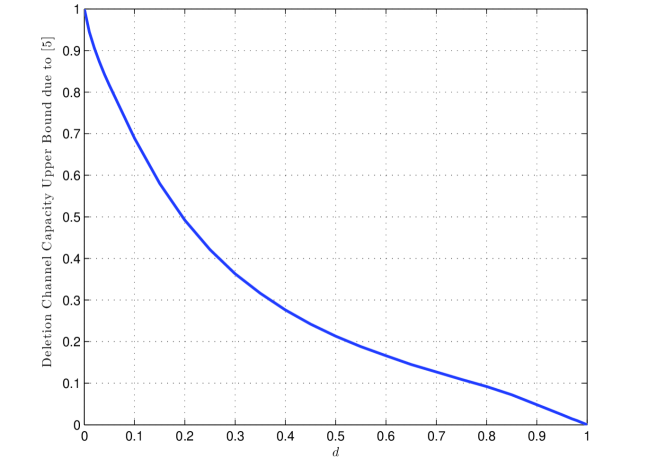
Figure 2: Previously best known upper bound on the i.i.d. deletion channel capacity.

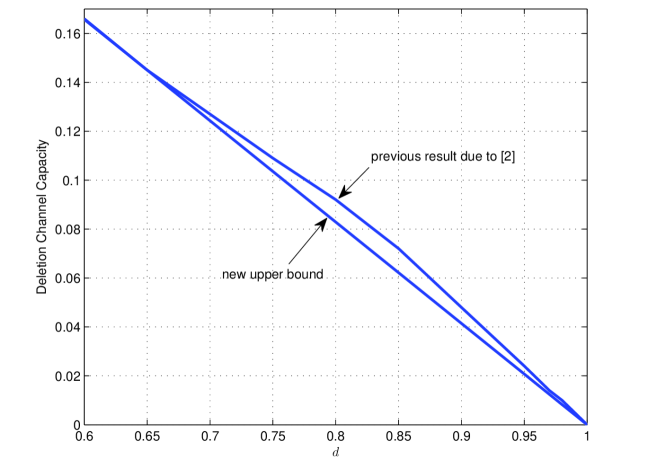
Figure 3: Improved upper bound on the deletion channel capacity employing $C(\lambda d+1-\lambda)\leq\lambda C(d)$.

We note that our result is a generalization of the one in [1] where it was shown that $C(d)\leq 0.4143(1-d)$ as $d\rightarrow 1$. We also note an earlier asymptotic result on a lower bound derived in [3] which states that $C(d)$ as $d\rightarrow 1$ is larger than $0.1185(1-d)$.

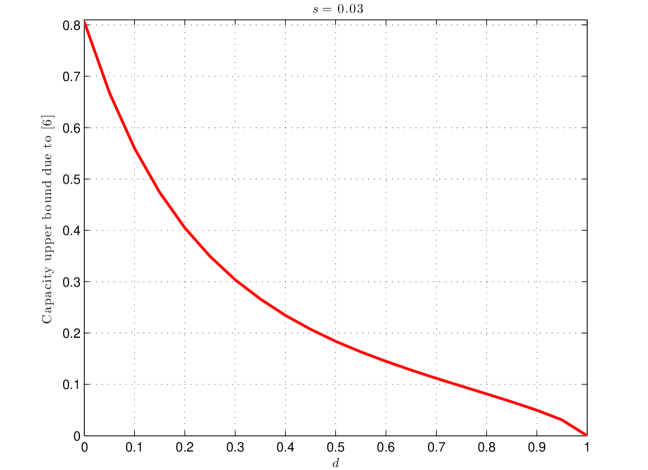
Figure 4: Previously best known upper bound on the deletion/substitution channel capacity for $s=0.03$.

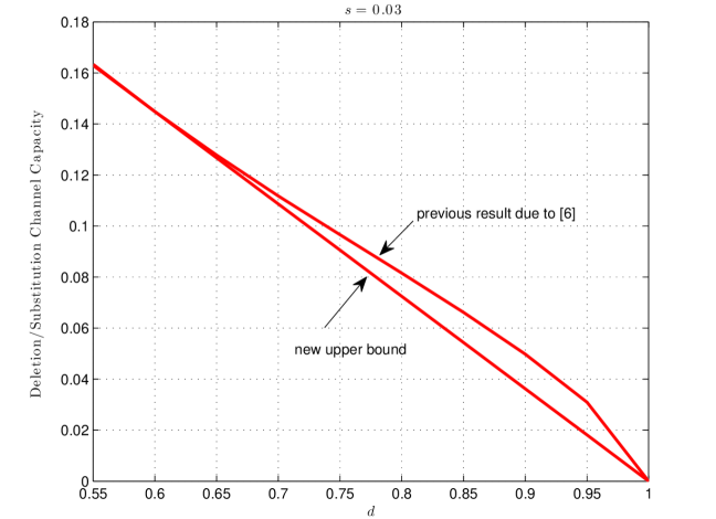
Figure 5: Improved upper bound on the deletion/substitution channel capacity for $s=0.03$.

As another application of the inequality derived in this paper, we can consider the capacity of the deletion/substitution channel. The best known capacity upper bound for this case is given in [7], e.g., Fig. 1 of [7] presents several upper bounds for fixed $s=0.03$ (see Fig. 4). It is clear that this bound is not a convex function of the deletion probability for $d\geq 0.6$, hence it can be improved. That is, applying the result in our paper, we obtain, for instance for $s=0.03$, $C_{s}(d,0.03)\leq 0.3621(1-d)$ for $d\geq 0.6$ which is a tighter bound as illustrated in Fig. 5.

V Conclusions

In this paper, an inequality relating the capacity of a deletion channel to two other deletion channels is found. The main idea is to consider parallel concatenation of two different independent deletion channels and relate the capacity of the resulting deletion channel with the capacity of the first two. An immediate application of this result is in obtaining improved upper bounds on the capacity of the deletion channel as the best available upper bounds are not convex in the deletion probability, and the derived inequality results in a tighter capacity characterization. For an i.i.d. deletion channel, we proved that $C(d)\geq 0.4143(1-d)$ for all $d\geq 0.65$. This is a stonger result than the earlier characterization in [1] which is valid only asymptotically as $d\rightarrow 1$. We also noted a generalization of the result to the case of a deletion/substitution channel and provided a tigher capacity upper bound for this case as well.

Appendix A Stochastic Properties of $\mbox{\boldmath$M$}_{1}$ and $\mbox{\boldmath$M$}_{2}$

For $P(\mbox{\boldmath$M$}_{1},\mbox{\boldmath$M$}_{2})$, we can write

$$P(\mbox{\boldmath$M$}_{1}=M_{1},\mbox{\boldmath$M$}_{2}=M_{2}) =\sum_{N_{1}=M_{1}}^{N-M_{2}}P(\mbox{\boldmath$M$}_{1}=M_{1},\mbox{\boldmath$M$}_{2}=M_{2}|\mbox{\boldmath$N$}_{1}=N_{1})P(\mbox{\boldmath$N$}_{1}=N_{1})$$

$$=\sum_{N_{1}=M_{1}}^{N-M_{2}}P(\mbox{\boldmath$M$}_{1}=M_{1}|\mbox{\boldmath$N$}_{1}=N_{1})P(\mbox{\boldmath$M$}_{2}=M_{2}|\mbox{\boldmath$N$}_{1}=N_{1})P(\mbox{\boldmath$N$}_{1}=N_{1})$$

$$=\sum_{N_{1}=M_{1}}^{N-M_{2}}{{N_{1}}\choose{M_{1}}}d_{1}^{N_{1}-M_{1}}(1-d_{1})^{M_{1}}{{N-N_{1}}\choose{M_{2}}}d_{2}^{N-N_{1}-M_{2}}(1-d_{2})^{M_{2}}\times$$

$$\quad\quad\quad\quad\times{N\choose{N_{1}}}\lambda^{N_{1}}(1-\lambda)^{N-N_{1}}$$

$$={{N-M_{2}}\choose{M_{1}}}{N\choose{M_{2}}}(\lambda(1-d_{1}))^{M_{1}}((1-\lambda)(1-d_{2}))^{M_{2}}\times$$

$$\quad\times\sum_{N_{1}=M_{1}}^{N-M_{2}}{{N-(M_{1}+M_{2})}\choose{N_{1}-M_{1}}}(\lambda d_{1})^{N_{1}-M_{1}}((1-\lambda)d_{2})^{N-N_{1}-M_{2}}$$

$$={{N-M_{2}}\choose{M_{1}}}{N\choose{M_{2}}}(\lambda(1-d_{1}))^{M_{1}}((1-\lambda)(1-d_{2}))^{M_{2}}d^{N-M_{1}-M_{2}}.$$ (17)

Furthermore, due to the structure of the channel $\cal{C}^{\prime}$, $\mbox{\boldmath$M$}_{2}$ is binomially distributed, i.e., $P(\mbox{\boldmath$M$}_{2}=M_{2})={N\choose{M_{2}}}((1-\lambda)(1-d_{2}))^{M_{2}}(\lambda+(1-\lambda)d_{2})^{N-M_{2}}$, and as a result $E\{\mbox{\boldmath$M$}_{2}\}=N(1-\lambda)(1-d_{2})$. On the other hand, to obtain $E_{\mbox{\boldmath$M$}_{1}}\{\mbox{\boldmath$M$}_{1}|\mbox{\boldmath$M$}_{2}\}$, we first need to obtain $P(\mbox{\boldmath$M$}_{1}|\mbox{\boldmath$M$}_{2})$, for which we can write

$$P(\mbox{\boldmath$M$}_{1}=M_{1}|\mbox{\boldmath$M$}_{2}=M_{2}) =\frac{P(\mbox{\boldmath$M$}_{1},\mbox{\boldmath$M$}_{2})}{P(\mbox{\boldmath$M$}_{2})}$$

$$={{N-M_{2}}\choose{M_{1}}}(\lambda(1-d_{1}))^{M_{1}}(\lambda d_{1}+(1-\lambda)d_{2})^{N-M_{1}-M_{2}}(\lambda+(1-\lambda)d_{2})^{M_{2}-N}.$$

Therefore, we obtain

$$E_{\mbox{\boldmath$M$}_{1}}\{\mbox{\boldmath$M$}_{1}|\mbox{\boldmath$M$}_{2}\} =\sum_{M_{1}=0}^{N-M_{2}}M_{1}{{N-M_{2}}\choose{M_{1}}}(\lambda(1-d_{1}))^{M_{1}}(\lambda d_{1}+(1-\lambda)d_{2})^{N-M_{1}-M_{2}}(\lambda+(1-\lambda)d_{2})^{M_{2}-N}$$

$$=(N-M_{2})\frac{\lambda(1-d_{1})}{\lambda+(1-\lambda)d_{2}}.$$ (18)

References

• [1] M.Β Dalai, β€œA new bound on the capacity of the binary deletion channel with high deletion probabilities,” in Proc. IEEE Int. Symp. Inf. Theory (ISIT), pp. 499–502, Aug. 2011.
• [2] R.Β L. Dobrushin, β€œShannon’s theorems for channels with synchronization errors,” Probs. Inf. Transm., vol.Β 3, no.Β 4, pp. 11–26, 1967.
• [3] M.Β Mitzenmacher and E.Β Drinea, β€œA simple lower bound for the capacity of the deletion channel,” IEEE Trans. Inf. Theory, vol.Β 52, no.Β 10, pp. 4657–4660, 2006.
• [4] E.Β Drinea and M.Β Mitzenmacher, β€œImproved lower bounds for the capacity of i.i.d. deletion and duplication channels,” IEEE Trans. Inf. Theory, vol.Β 53, no.Β 8, pp. 2693–2714, Aug. 2007.
• [5] A.Β Kirsch and E.Β Drinea, β€œDirectly lower bounding the information capacity for channels with i.i.d. deletions and duplications,” IEEE Trans. Inf. Theory, vol.Β 56, no.Β 1, pp. 86 –102, Jan. 2010.
• [6] D.Β Fertonani and T.Β M. Duman, β€œNovel bounds on the capacity of the binary deletion channel,” IEEE Trans. Inf. Theory, vol.Β 56, no.Β 6, pp. 2753–2765, June 2010.
• [7] D.Β Fertonani, T.Β M. Duman, and M.Β F. Erden, β€œBounds on the capacity of channels with insertions, deletions and substitutions,” IEEE Trans. on Communications, vol.Β 59, no.Β 1, pp. 2–6, Jan. 2011.
• [8] M.Β Rahmati and T.Β M. Duman, β€œAnalytical lower bounds on the capacity of insertion and deletion channels,” submitted to IEEE Trans. Inf. Theory, ArXiv e-prints:1101.1310[cs.IT], Jan. 2011.
• [9] β€”β€”, β€œAchievable rates for noisy channels with synchronization errors,” submitted to IEEE Trans. Inf. Theory, ArXiv e-prints:1203.6396[cs.IT], Mar. 2012.
• [10] T.Β M. Cover and J.Β A. Thomas, Elements of Information Theory.Β Β Β Wiley, 2006.
• [11] S.Β Diggavi, M.Β Mitzenmacher, and H.Β Pfister, β€œCapacity upper bounds for deletion channels,” in Proceedings of the International Symposium on Information Theory (ISIT), 2007, pp. 1716–1720.