A General Framework for Consistency of Principal Component Analysis

Abstract

A general asymptotic framework is developed for studying consistency properties of principal component analysis (PCA). Our framework includes several previously studied domains of asymptotics as special cases and allows one to investigate interesting connections and transitions among the various domains. More importantly, it enables us to investigate asymptotic scenarios that have not been considered before, and gain new insights into the consistency, subspace consistency and strong inconsistency regions of PCA and the boundaries among them. We also establish the corresponding convergence rate within each region. Under general spike covariance models, the dimension (or the number of variables) discourages the consistency of PCA, while the sample size and spike information (the relative size of the population eigenvalues) encourages PCA consistency. Our framework nicely illustrates the relationship among these three types of information in terms of dimension, sample size and spike size, and rigorously characterizes how their relationships affect PCA consistency.

, and

m1Corresponding Author t1Partially supported by NSF grant DMS-0854908 t2Partially supported by NSF grants DMS-1106912 and CMMI-0800575, NIH Challenge Grant 1 RC1 DA029425-01, and the Xerox Foundation UAC Award t3Partially supported by NSF grants DMS-0606577 and DMS-0854908

1 Introduction

Principal Component Analysis (PCA) is an important visualization and dimension reduction tool which finds orthogonal directions reflecting maximal variation in the data. This allows the low dimensional representation of data, by projecting data onto these directions. PCA is usually obtained by an eigen decomposition of the sample variance-covariance matrix of the data. Properties of the sample eigenvalues and eigenvectors have been analyzed under several domains of asymptotics.

In this paper, we develop a general asymptotic framework to explore interesting transitions among the various asymptotic domains. The general framework includes the traditional asymptotic setups as special cases, which allows careful study of the connections among the various setups, and more importantly it investigates scenarios that have not been considered before, and offers new insights into the consistency (in the sense that the angle between estimated and population eigen direction tends to 0, or the inner product tends to 1) and strong-inconsistency (where the angle tends to $\frac{\pi}{2}$, i.e., the inner product tends to 0) properties of PCA, along with some technically challenging convergence rates.

Existing asymptotic studies of PCA roughly fall into three domains:

1. the classical domain of asymptotics, under which the sample size $n\rightarrow\infty$ and the dimension $d$ is fixed (hence the ratio $\frac{n}{d}\rightarrow\infty$). For example, see [11, 19, 2, 3, 14].

2. the random matrix theory domain, where both the sample size $n$ and the dimension $d$ increase to infinity, with the ratio $\frac{n}{d}\rightarrow c$, a constant mostly assumed to be within $(0,\infty)$. Representative work includes [9, 29, 26, 13] from the statistical physics literature, as well as [15, 4, 5, 22, 23, 21, 16, 20, 8] from the statistics literature.

3. the high dimension low sample size (HDLSS) domain of asymptotics, which is based on the limit, as the dimension $d\rightarrow\infty$, with the sample size $n$ being fixed (hence the ratio $\frac{n}{d}\rightarrow 0$). HDLSS asymptotics was originally studied by [10], and recently rediscovered by [12]. PCA has been studied using the HDLSS asymptotics by [1, 17].

PCA consistency and (strong) inconsistency, defined in terms of angles, are important properties that have been studied before. A common technical device is the spike covariance model, initially introduced by Johnstone [15]. This model has been used in this context by, for example, Nadler [21], Johnstone and Lu [16], and Jung and Marron [17]. An interesting, more general model has been considered by Benaych-Georges and Nadakuditi [8].

Under the spike model, the first few eigenvalues are much larger than the others. A major point of the present paper is that there are three critical features whose relationships drive the consistency properties of PCA, namely

1. the sample information: the sample size $n$, which has a positive contribution to, i.e. encourages, the consistency of the sample eigenvectors.

2. the variable information: the dimension $d$, which has a negative contribution to, i.e. discourages, the consistency of the sample eigenvectors.

3. the spike information: the relative sizes of the several leading eigenvalues, which also has a positive contribution to the consistency.

Our general framework considers increasing sample size $n$, increasing dimension $d$, and increasing spike information. It clearly characterizes how their relationships determine the regions of consistency and strong-inconsistency of PCA, along with the boundary in-between. In addition, our theorems demonstrate the transitions among the existing domains of asymptotics, and for the first time to the best of our knowledge, enable one to understand the connections among them. Note that the classical domain ((a) above) assumes increasing sample size $n$ while fixing dimension $d$; the random matrix domain ((b) above) assumes increasing sample size $n$ and increasing dimension $d$, while fixing the spike information; the HDLSS domain ((c) above) fixes the sample size, and increases the dimension and the spike information; thus each of these three domains is a boundary case of our framework. Finally, our theorems also contain novel results on rates of convergence.

Sections 3 and 4 formally state very general theorems for the single and multiple component spike models, respectively. For illustration purposes only, in this section we first consider Examples 1.1 and 1.2 under some strong assumptions, which provide intuitive insight regarding the much more general theory presented in Sections 3 and 4.

For these two illustrative examples, the three types of information and their relationships can be mathematically quantified by two indices, namely the spike index $\alpha$ and the sample index $\gamma$. Within the context of these examples, we point out the significant contributions of our results in comparison with existing results. The comparisons and connections are graphically illustrated in Figure 1 and discussed below.

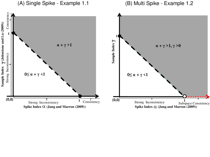
Figure 1: General consistency and strong inconsistency regions for PCA, as a function of the spike index $\alpha$ and the sample index $\gamma$. Panel (A) - single spike model in Example 1.1: PCA is consistent on the grey region ($\alpha+\gamma>1$), and strongly inconsistent on the white triangle ($0\leq\alpha+\gamma<1$). Panel (B) - multiple spike model in Example 1.2: the first $m$ sample PCs are consistent on the grey region ($\alpha+\gamma>1,\gamma>0$), subspace consistent on the dotted line segment ($\alpha>1,\gamma=0$) on the horizontal axis, and strongly inconsistent on the white triangle ($0\leq\alpha+\gamma<1$).

Example 1.1.

(Single-component spike model) Assume that $X_{1},\ldots,X_{n}$ are random sample vectors from a $d$-dimensional normal distribution $N(0,\Sigma)$, where the sample size $n\sim d^{\gamma}$ ($\gamma\geq 0$ is defined as the sample index) and the covariance matrix $\Sigma$ has the eigenvalues as

$$\lambda_{1}\sim d^{\alpha},\lambda_{2}=\cdots=\lambda_{d}=1,\alpha\geq 0,$$

where the constant $\alpha$ is defined as the spike index.

Theorem 3.1, when applied to this example, suggests that the maximal sample eigenvector is consistent when $\alpha+\gamma>1$ (grey region in Figure 1(A)), and strongly inconsistent when $0\leq\alpha+\gamma<1$ (white triangle in Figure 1(A)). These very general new results nicely connect with many existing ones:

• Previous Results I - the classical domain:

  For this example, Theorem 1 of Anderson [2] implied that for fixed dimension $d$ and finite eigenvalues, when the sample size $n\rightarrow\infty$ (i.e. $\gamma\rightarrow\infty$, the limit on the vertical axis), the maximal sample eigenvector is consistent. This case is the upper left corner of Figure 1(A).

• Previous Results II - the random matrix domain:

  1. The results of Johnstone and Lu [16] appear on the vertical axis in Panel (A) where the spike index $\alpha=0$ (as they fix the spike information): the first sample eigenvector is consistent when the sample index $\gamma>1$ and strongly inconsistent when $\gamma<1$.

  2. Nadler [21] explored the interesting boundary case of $\alpha=0,\gamma=1$ (i.e. $\frac{d}{n}\rightarrow c$ for a constant $c$) and showed that $<\hat{u}_{1},u_{1}>^{2}\xrightarrow{\rm a.s}\frac{((\lambda_{1}-1)^{2}-c)_{+}}{(\lambda_{1}-1)^{2}+c(\lambda_{1}-1)}$, where $\hat{u}_{1}$ and $u_{1}$ are the first sample and population eigenvector. This result appears in Panel (A) as the single solid circle $\gamma=1$ on the vertical axis.

• Previous Results III - the HDLSS domain:

  1. The theorems of Jung and Marron [17] are represented on the horizontal axis in Panel (A) when the sample index $\gamma=0$ (as they fix the sample size): the maximal sample eigenvector is consistent with the first population eigenvector when the spike index $\alpha>1$ and strongly inconsistent when $\alpha<1$.

  2. Jung et al. [18] deeply explored limiting behavior at the boundary $\alpha=1,\gamma=0$ (i.e. $\frac{d}{\lambda_{1}}\rightarrow c$ for a constant $c$) and showed that $<\hat{u}_{1},u_{1}>^{2}\Rightarrow\frac{\chi_{n}^{2}}{\chi_{n}^{2}+c}$, where $``\Rightarrow"$ means convergence in distribution and $\chi_{n}^{2}$ is the chi-squared distribution with $n$ degrees of freedom. This result appears in Panel (A) as the single solid circle $\alpha=1$ on the horizontal axis.

• Our Results hence nicely connect existing domains of asymptotics, and give a much more complete characterization for the regions of PCA consistency, subspace consistency, and strong inconsistency. We also investigate asymptotic properties of the other sample eigenvectors and all the sample eigenvalues.

Example 1.2.

(Multiple-component spike model) Assume that the covariance matrix $\Sigma$ in Example 1.1 has the following eigenvalues

$$\lambda_{j}=\begin{cases}c_{j}d^{\alpha}&\text{if $j\leq m$,}\\ 1&\text{if $j>m$,}\end{cases}\quad{\alpha\geq 0},$$

where $m$ is a finite positive integer, the constants $c_{j},j=1,\cdots,m$, are positive and satisfy that $c_{j}>c_{j+1}>1$, $j=1,\cdots,m-1$.

Theorem 4.1, when applied to this example, shows that the first $m$ sample eigenvectors are individually consistent with corresponding population eigenvectors when $\alpha+\gamma>1,\gamma>0$ (the grey region in Figure 1(B)), instead of being subspace consistent [17], and strongly inconsistent when $\alpha+\gamma<1$ (the white triangle in Panel (B)). This very general new result connects with many others in the existing literature:

• Previous Results I - the classical domain:

  For this example, Theorem 1 of Anderson [2] implied that for fixed dimension $d$ and finite eigenvalues, when the sample size $n\rightarrow\infty$ (i.e. $\gamma\rightarrow\infty$, the limit on the vertical axis), the first $m$ sample eigenvectors are consistent, while the other sample eigenvectors are subspace consistent. This case is the upper left corner of Figure 1(B).

• Previous Results II - the random matrix domain:

  Paul [23] explored asymptotic properties of the first $m$ eigenvectors and eigenvalues in the interesting boundary case of $\alpha=0,\gamma=1$, i.e., $\frac{d}{n}\rightarrow c$ with $c\in(0,1)$ and showed that $<\hat{u}_{j},u_{j}>^{2}\xrightarrow{\rm a.s}\frac{((\lambda_{j}-1)^{2}-c)_{+}}{(\lambda_{j}-1)^{2}+c(\lambda_{j}-1)}$ for $j=1,\cdots,m$. This result appears in Panel (B) as the solid circle $\gamma=1$ on the vertical axis. Paul and Johnstone [24] considered a similar framework but from a minimax risk analysis perspective. Nadler [21] and Johnstone and Lu [16] did not study multiple spike models.

• Previous Results III - the HDLSS domain:

  The theorems of Jung and Marron [17] are valid on the horizontal axis in Panel (B) where the sample index $\gamma=0$. In particular, for this example, their results showed that the first $m$ sample eigenvectors are not separable when the spike index $\alpha>1$ (the horizontal dotted red line segment), instead they are subspace consistent with their corresponding population eigenvectors, and are strongly inconsistent when the spike index $\alpha<1$ (the horizontal solid line segment). They and Jung et al. [18] did not study the asymptotic behavior on the boundary - the single open circle $(\alpha=1,\gamma=0)$ on the horizontal axis.

• Our Results cover the classical domain, and are stronger than what [17] obtained: the increasing sample size enables us to separate out the first few leading eigenvectors and characterize individual consistency, while only subspace consistency was obtained by [17].

The organization of the rest of the paper is as follows. Section 2 first introduces our notations and several relevant consistency concepts. Section 3 then presents the theoretical results of single-component spike models, stating the asymptotic properties of the sample eigenvalues and eigenvectors under our general framework. Section 3.1 first considers single-component spike models with the increasing sample size $n$, and Section 3.2 then studies single-component spike models where the sample size $n$ is fixed. Section 4 studies multiple-component spike models. For easy access to the main ideas, Section 4.1 first studies models with distinct eigenvalues, while Section 4.2 then considers models where the eigenvalues are grouped. Section 5 contains some discussion about the asymptotic properties of PCA when some small eigenvalues equal to zero and the challenges to obtain non-asymptotic results. Section 6 contains the technical proofs of the main theorem.

2 Notations and Concepts

We now introduce some necessary notations, and define consistency concepts relevant for our asymptotic study.

2.1 Notation

Let the population covariance matrix be $\Sigma$, whose eigen decomposition is

$$\Sigma=U\Lambda U^{T},$$

where $\Lambda$ is the diagonal matrix of population eigenvalues $\lambda_{1}\geq\lambda_{2}\geq\ldots\geq\lambda_{d}$, and $U$ is the matrix of corresponding eigenvectors $U=[u_{1},\ldots,u_{d}]$.

As in Jung and Marron [17], assume that $X_{1},\ldots,X_{n}$ are i.i.d. $\;d$-dimensional random sample vectors and have the following representation

$$~{}X_{i}=\sum_{j=1}^{d}z_{i,j}u_{j},$$ (2.1)

where the $z_{i,j}$’s are i.i.d random variables with zero mean, unit variance and finite fourth moment. An important special case is that the $z_{i,j}$’s follow the standard normal distribution $N(0,1)$.

Assumption 2.1.

$X_{1},\ldots,X_{n}$ are a random sample having the distribution described by  (2.1).

Denote the sample covariance matrix by $\hat{\Sigma}=n^{-1}XX^{T}$, where $X=[X_{1},\ldots,X_{n}]$. Note that $\hat{\Sigma}$ can also be decomposed as

$$\hat{\Sigma}=\hat{U}\hat{\Lambda}\hat{U}^{T},$$ (2.2)

where $\hat{\Lambda}$ is the diagonal matrix of sample eigenvalues $\hat{\lambda}_{1}\geq\hat{\lambda}_{2}\geq\ldots\geq\hat{\lambda}_{d}$ and $\hat{U}$ is the matrix of corresponding sample eigenvectors where $\hat{U}=[\hat{u}_{1},\ldots,\hat{u}_{d}]$.

Below we introduce asymptotic notations that will be used in our theoretical studies. Assume that $\{\xi_{n}:n=1,\ldots,\infty\}$ is a sequence of random variables, and $\{a_{n}:n=1,\ldots,\infty\}$ is a sequence of constant values.

• Denote $\xi_{n}={\rm o}_{\rm a.s}\left(a_{n}\right)$ if $\mbox{lim}_{n\rightarrow\infty}\frac{\xi_{n}}{a_{n}}=0$ almost surely.

• Denote $\xi_{n}={\rm O}_{\rm a.s}\left(a_{n}\right)$ if $\overline{\mbox{lim}}_{n\rightarrow\infty}\left|\frac{\xi_{n}}{a_{n}}\right|\leq z$ almost surely, where the random variable $z$ satisfies $P(0<z<\infty)=1$..

• Denote $\xi_{n}\stackrel{{\scriptstyle\rm a.s}}{{\sim}}a_{n}$ if $c_{2}\leq\underline{\mbox{lim}}_{n\rightarrow\infty}\frac{\xi_{n}}{a_{n}}\leq\overline{\mbox{lim}}_{n\rightarrow\infty}\frac{\xi_{n}}{a_{n}}\leq c_{1}$ almost surely, for two constants $c_{1}\geq c_{2}>0$.

In addition, we introduce the following notions to help understand the assumptions on the population eigenvalues in our theorems. Assume that $\{a_{k}:k=1,\ldots,\infty\}$ and $\{b_{k}:k=1,\ldots,\infty\}$ are two sequence of constant values, where $k$ can stand for either $n$ or $d$.

• Denote $a_{k}\gg b_{k}$ if $\mbox{lim}_{k\rightarrow\infty}\frac{b_{k}}{a_{k}}=0$.

• Denote $a_{k}\sim b_{k}$ if $c_{2}\leq\underline{\mbox{lim}}_{k\rightarrow\infty}\frac{a_{k}}{b_{k}}\leq\overline{\mbox{lim}}_{k\rightarrow\infty}\frac{a_{k}}{b_{k}}\leq c_{1}$ for two constants $c_{1}\geq c_{2}>0$.

2.2 Concepts

Below we list three important concepts relevant for consistency and strong inconsistency, some of which are modified from the related concepts given by Jung and Marron [17] and Shen et al. [27].

Let $\hat{u}_{j}$ be any normalized sample estimator of $u_{j}$ for $j=1,\ldots,[n\wedge d]$.

• Consistency with rate $a_{n}$: The estimator $\hat{u}_{j}$ is consistent with its population counterpart $u_{j}$ with the convergence rate $a_{n}$ if $\mid<\hat{u}_{j},u_{j}>\mid=1+{\rm O}_{\rm a.s}(a_{n})$. For example, $a_{n}=\left(\frac{n\lambda_{1}}{d}\right)^{\frac{1}{2}}$.

• Strong inconsistency with rate $a_{n}$: $\hat{u}_{j}$ is strongly inconsistent with $u_{j}$ with the convergence rate $a_{n}$ if $|<\hat{u}_{j},u_{j}>|={\rm O}_{\rm a.s}(a_{n})$.

Let $H$ be an index set, e.g. $H=\{m+1,\cdots,d\}$. Define $S=\mbox{span}\{u_{k},k\in H\}$ to be the linear span generated by $\{u_{k},k\in H\}$.

• Subspace consistency with rate $a_{n}$: $\hat{u}_{j}$, $j\in H$, is subspace consistent with $S$ with convergence rate $a_{n}$ if

  $$\mbox{angle}(\hat{u}_{j},S)={\rm O}_{a.s}(a_{n}),$$ (2.3)

  where the angle between the estimator $\hat{u}_{j}$ and the subspace $S$ is the angle between the estimator and its projection onto the subspace, see Jung and Marron [17]. For further clarification, we provide a graphical illustration of the angle in Section B of the supplement [28].

Terminology: In the following results, for simple general formulations, the term - consistent at the rate $a_{n}$ - will mean $``{\rm O}_{\rm a.s}(a_{n})"$ in situations where $a_{n}\rightarrow 0$. Otherwise it means $``{\rm o}_{\rm a.s}(a_{n})"$. Similarly for strong inconsistency and subspace consistency.

3 Single component spike models

Below we state our main theorems for single-component spike models. In Section 3.1, we study the asymptotic properties of PCA with increasing sample size $n$. In Section 3.2 , we investigate the asymptotic properties of PCA with fixed $n$.

3.1 Cases with increasing sample size $n$

We first state in Theorem 3.1 one of our main theoretical results regarding PCA consistency under our general framework. We then offer several remarks in regards to the conditions of the theorem as well as the connection between our results and the earlier ones in the literature.

To fix ideas, we assume the maximal eigenvalue $\lambda_{1}$ dominates the other eigenvalues. WLOG, we assume that as $n\rightarrow\infty$ or $d\rightarrow\infty$,

Assumption 3.1.

$\lambda_{1}>\lambda_{2}\rightarrow\cdots\rightarrow\lambda_{d}\rightarrow c_{\lambda}$, where $c_{\lambda}$ is a constant.

As discussed in the Introduction, we consider the delicate balance among the positive sample information $n$, the positive spike information $\lambda_{1}$, and the negative variable information $d$, and characterize the various PCA consistency and strong-inconsistency regions.

Theorem 3.1 below suggests that the asymptotic properties of the sample eigenvalues and eigenvectors depend on the relative strength of the positive information and the negative information, as particularly measured by two ratios: $\frac{d}{n\lambda_{1}}$ and $\frac{d}{n}$. The value of $\frac{d}{n\lambda_{1}}$ determines whether the maximal sample eigenvalue is separable from the other eigenvalues, and further determines the consistency of the maximal sample eigenvector. The value of $\frac{d}{n}$ determines the asymptotic properties of the second and higher sample eigenvalues and eigenvectors.

The following discussion and the scenarios in Theorem 3.1 are arranged according to a decreasing amount of positive information:

• Theorem 3.1(a): If the amount of positive information dominates the amount of negative information up to the maximal eigenvalue, i.e. $\frac{d}{n\lambda_{1}}\rightarrow 0$, then the maximal sample eigenvector is consistent, and the other sample eigenvectors are subspace consistent. In addition, the asymptotic properties of sample eigenvalues and eigenvectors whose index are greater than 1 depend on the value $\frac{d}{n}$.

• Theorem 3.1(b): On the other hand, if the amount of negative information always dominates, i.e. $\frac{d}{n\lambda_{1}}\rightarrow\infty$, then the sample eigenvalues are asymptotically indistinguishable, and the sample eigenvectors are strongly inconsistent.

Theorem 3.1.

Under Assumptions 2.1 and 3.1, as $n\rightarrow\infty$, the following results hold.

1. If $\frac{d}{n\lambda_{1}}\rightarrow 0$, then $\frac{\hat{\lambda}_{1}}{\lambda_{1}}\xrightarrow{\rm a.s}1$, $\hat{u}_{1}$ is consistent with $u_{1}$, and the other $\hat{u}_{j}$ are subspace consistent with $S=\mbox{span}\{u_{k},k\geq 2\}$. In addition,

   1. If $\frac{d}{n}\rightarrow 0$, then $\frac{\hat{\lambda}_{j}}{\lambda_{j}}\xrightarrow{\rm a.s}1$, $j=2,\cdots,[n\wedge(d-1)]$, and $\hat{\lambda}_{[n\wedge d]}={\rm O}_{\rm a.s}(1)$. The consistency rate for $\hat{u}_{1}$ and the subspace consistency rate for the other $\hat{u}_{j}$ are both $\left(\frac{1}{\lambda_{1}}\right)^{\frac{1}{2}}$.

   2. If $\frac{d}{n}\rightarrow\infty$, then $\frac{\hat{\lambda}_{j}}{\lambda_{j}}\stackrel{{\scriptstyle\rm a.s}}{{\rightarrow}}\frac{d}{n}$ for $j=2,\cdots,[n\wedge d]$; $\hat{u}_{1}$ is consistent with rate $\left(\frac{d}{n\lambda_{1}}\right)^{\frac{1}{2}}$, and the other $\hat{u}_{j}$ are strongly inconsistent with rate $\left(\frac{n\lambda_{j}}{d}\right)^{\frac{1}{2}}$.

   3. If $\overline{{\rm lim}}\frac{d}{n}=c^{*}$ ($0<c^{*}\leq\infty$), then for $j=2,\cdots,[n\wedge d]$, $\overline{{\rm lim}}\hat{\lambda}_{j}\leq c\times\overline{{\rm lim}}\frac{d}{n}$ almost surely, where $c$ is some constant. The consistency rate for $\hat{u}_{1}$ and the subspace consistency rate for the other $\hat{u}_{j}$ are both $\left(\frac{d_{n}}{n\lambda_{1}}\right)^{\frac{1}{2}}$, where $\{d_{n}\}$ is a sequence converging to $c^{*}$.

2. If $\frac{d}{n\lambda_{1}}\rightarrow\infty$, then $\hat{\lambda}_{j}\stackrel{{\scriptstyle\rm a.s}}{{\rightarrow}}c_{\lambda}\frac{d}{n}$ for $j=1,\cdots,[n\wedge d]$, and the corresponding eigenvectors $\hat{u}_{j}$ are strongly inconsistent with rate $(\frac{n\lambda_{j}}{d})^{\frac{1}{2}}$.

Having stated the main results for single-component spike models, we now offer several remarks regarding the conditions assumed in Theorem 3.1 and make connections with existing results about PCA consistency.

• If Assumption 3.1 is replaced by the alternative assumption $\lambda_{1}\gg\lambda_{2}\sim\cdots\lambda_{d}\sim 1$, then except for $\frac{\hat{\lambda}_{1}}{\lambda_{1}}\xrightarrow{\rm a.s}1$ in Scenario (a), all other $``\xrightarrow{\rm a.s}"$ for the sample eigenvalues should be replaced by $``\stackrel{{\scriptstyle\rm a.s}}{{\sim}}"$. The results for the sample eigenvectors remain the same.

• An assumption of the form (3.1), i.e $\lambda_{2}\rightarrow\cdots\rightarrow\lambda_{d}\rightarrow c_{\lambda}$, or else $\lambda_{2}\sim\cdots\lambda_{d}\sim 1$ is needed to obtain general convergence results for the non-spike sample eigenvalues $\hat{\lambda}_{j}$, $j>1$ under the wide range of scenarios: $\frac{d}{n}\rightarrow 0$, $\frac{d}{n}\rightarrow\infty$ or $\overline{{\rm lim}}\frac{d}{n}=c^{*}$ ($0<c^{*}\leq\infty$). When one focusses only on the spike eigenvalue, a weaker assumption, such as the slowly decaying non-spike eigenvalues assumed by Bai and Yao (2012) [7], is enough. Then the spike condition $\lambda_{1}\gg\lambda_{2}$ is enough to generate the consistency properties of $\hat{\lambda}_{1}$ and $\hat{u}_{1}$ in Scenario (a). In that case, the behaviors of the other sample eigenvalues and eigenvectors are very case-wise to formulate in general.

• Nadler [21] and Johnstone and Lu (2009) [16] studied the properties of the first sample eigenvalue and eigenvector under the normality assumption for fixed $\lambda_{1}$. Furthermore, if $d$ is fixed, Scenario (a) of Theorem 3.1 degenerates to the case studied by Anderson (1963) [2].

• Assuming fixed $\lambda_{1}$ and $\frac{d}{n}\rightarrow c$ with $c$ being a constant, Nadler [21], Johnstone and Lu [16] and Benaych-Georges and Nadakuditi [8] obtained the results in Previous Results II - the random matrix domain in Example 1.1, which indicate that, as $n\rightarrow\infty$, the maximal sample eigenvector $\hat{u}_{1}$ is consistent when $\frac{d}{n}\rightarrow 0$, and inconsistent when $\frac{d}{n}\rightarrow\infty$. Our Theorem 3.1 includes this as a special case. In addition, Theorem 3.1 offers more than just relaxing the fixed $\lambda_{1}$ assumption: it characterizes how an increasing $\lambda_{1}$ interacts with the ratio $\frac{d}{n}$, derives the corresponding convergence rate, and also studies the asymptotic properties of the higher order sample eigenvalues and eigenvectors, all of which have not been investigated before.

3.2 Cases with fixed $n$

Theorem 3.2 summarize the results for the fixed $n$ cases (i.e. the HDLSS domain). In comparison with Jung and Marron (2009) [17], we make more general assumptions on the population eigenvalues, and obtain the corresponding convergence rate results; furthermore, we obtain almost sure convergence, instead of convergence in probability [17].

Consider the $z_{i,j}$ in (2.1), and define

$$\widetilde{Z}_{j}=(z_{1,j},\cdots,z_{n,j})^{T},\quad j=1,\cdots,d,$$ (3.1)

which are needed here to describe the asymptotic properties of the sample eigenvalues in HDLSS settings. In addition, define $K=\lim_{d\rightarrow\infty}\frac{\sum_{j=2}^{d}\lambda_{j}}{nd}$.

Theorem 3.2.

Under Assumptions 2.1 and 3.1, for fixed $n$, as $d\rightarrow\infty$, the following results hold.

1. If $\frac{d}{\lambda_{1}}\rightarrow 0$, then $\frac{\hat{\lambda}_{1}}{\lambda_{1}}\stackrel{{\scriptstyle\rm a.s}}{{\rightarrow}}\frac{\widetilde{Z}_{1}^{T}\widetilde{Z}_{1}}{n}$, where $\widetilde{Z}_{1}$ is defined in (3.1), and the rest of the non-zero $\frac{\hat{\lambda}_{j}}{d}\stackrel{{\scriptstyle\rm a.s}}{{\rightarrow}}K$. In addition, $\hat{u}_{1}$ is consistent with rate $\left(\frac{d}{\lambda_{1}}\right)^{\frac{1}{2}}$, and the rest of the $\hat{u}_{j}$ are strongly inconsistent with rate $\left(\frac{\lambda_{j}}{d}\right)^{\frac{1}{2}}$.

2. If $\frac{d}{\lambda_{1}}\rightarrow\infty$, then the non-zero $\frac{\hat{\lambda}_{j}}{d}\stackrel{{\scriptstyle\rm a.s}}{{\rightarrow}}K$, and the corresponding $\hat{u}_{j}$ are strongly inconsistent with rate $(\frac{\lambda_{j}}{d})^{\frac{1}{2}}$, respectively.

Some comments about the conditions and results of Theorem 3.2

• Assumption 3.1 can be replaced by $\lambda_{1}\gg\lambda_{2}\sim\cdots\lambda_{d}\sim 1$. The results remain the same.

• Even if the non-spike eigenvalues $\lambda_{j}$, $j>2$, decay slowly, the condition $\lambda_{1}\gg\lambda_{2}$ is enough to generate the same properties for $\hat{\lambda}_{1}$ and $\hat{u}_{1}$ as in Scenario (a).

• If Assumption 2.1 is strengthened to a normality assumption, then $\frac{\hat{\lambda}_{1}}{\lambda_{1}}\stackrel{{\scriptstyle\rm a.s}}{{\rightarrow}}\frac{\chi_{n}^{2}}{n}$ in Scenario (a).

• Assumption 2.1 assumes that the $z_{i,j}$’s are i.i.d rather than $\rho$-mixing as in [17]. Thus, convergence in probability in [17] is strengthened to almost sure convergence here.

4 Multiple component spike models

We consider multiple spike models with finite $m(\in[1,n\wedge d])$ dominating spikes. In Section 4.1, we study models where the dominating eigenvalues are distinct. In Section 4.2, we consider the cases where the eigenvalues are not all distinct, by introducing the concept of tiered eigenvalues.

4.1 Multiple component spike models with distinct eigenvalues

4.1.1 Cases with increasing sample size $n$

WLOG, we assume that the first $m$ population eigenvalues have different strength and dominate the rest population eigenvalues, which are asymptotically equivalent.

Assumption 4.1.

as $n\rightarrow\infty$, $\lambda_{1}>\cdots>\lambda_{m}>\lambda_{m+1}\rightarrow\cdots\rightarrow\lambda_{d}\rightarrow c_{\lambda}.$

A useful quantity, for distinguishing the various cases among eigenvectors in the coming theorems, is

$$a_{l}=\mbox{max}_{1\leq k\leq l}\frac{\lambda_{k+1}}{\lambda_{k}},\quad l=1,\cdots,m.$$

This lower bound on the consecutive relative gap among the first $l$ eigenvalues provides a critical measure of the separation between the $l$-th sample eigenvector and the first $l-1$ sample eigenvectors.

Below we first state the main theoretical results in Theorem 4.1, and follow up with some remarks about the theorem conditions and the connections between the theorem and the existing results in the literature.

Similar to Theorem 3.1, Theorem 4.1 states the asymptotic properties of the sample eigenvalues and eigenvectors in a trichotomous manner, separated by the size of $\frac{d}{n\lambda_{j}}$, which again measures the relative strength of the positive information and the negative information. The three scenarios below and in Theorem 4.1 are arranged in a decreasing order of the amount of the positive information:

• Theorem 4.1(a): If the amount of positive information dominates the amount of negative information up to the $m$th spike, i.e. $\frac{d}{n\lambda_{m}}\rightarrow 0$, then each of the first $m$ sample eigenvector is consistent, and the additional ones are subspace consistent;

• Theorem 4.1(b): Otherwise, if the amount of positive information dominates the amount of negative information only up to the $h$th spike $(h\in[1,m])$, i.e. $\frac{d}{n\lambda_{h}}\rightarrow 0$ and $\frac{d}{n\lambda_{h+1}}\rightarrow\infty$, then each of the first $h$ sample eigenvector is consistent, and each of the remaining higher-order sample eigenvector is strongly-inconsistent;

• Theorem 4.1(c): Finally, if the amount of negative information always dominates, i.e. $\frac{d}{n\lambda_{1}}\rightarrow\infty$, then the sample eigenvalues are asymptotically indistinguishable, and the sample eigenvectors are strongly inconsistent.

Theorem 4.1.

Under Assumptions 2.1 and 4.1, as $n\rightarrow\infty$, the following results hold.

1. If $\frac{d}{n\lambda_{m}}\rightarrow 0$, then $\frac{\hat{\lambda}_{j}}{\lambda_{j}}\xrightarrow{\rm a.s}1$ for $1\leq j\leq m$. In addition, $\hat{u}_{j}$ are consistent with $u_{j}$ for $1\leq j\leq m$ and the other $\hat{u}_{j}$ are subspace consistent with $S=\mbox{span}\{u_{k},k\geq m+1\}$.

2. If there exists a constant $h$, $1\leq h\leq m$, such that $\frac{d}{n\lambda_{h}}\rightarrow 0$ and $\frac{d}{n\lambda_{h+1}}\rightarrow\infty$, then $\frac{\hat{\lambda}_{j}}{\lambda_{j}}\xrightarrow{\rm a.s}1$ for $1\leq j\leq h$, and the other non-zero $\hat{\lambda}_{j}\stackrel{{\scriptstyle\rm a.s}}{{\rightarrow}}c_{\lambda}\frac{d}{n}$. In addition, $\hat{u}_{j}$ are consistent with rate $\left(a_{j}\vee\frac{d}{n\lambda_{j}}\right)^{\frac{1}{2}}$ for $1\leq j\leq h$, and the other $\hat{u}_{j}$ are strongly inconsistent with rate $\left(\frac{n\lambda_{j}}{d}\right)^{\frac{1}{2}}$.

3. If $\frac{d}{n\lambda_{1}}\rightarrow\infty$, then the non-zero $\hat{\lambda}_{j}\stackrel{{\scriptstyle\rm a.s}}{{\rightarrow}}c_{\lambda}\frac{d}{n}$, and the corresponding $\hat{u}_{j}$ are strongly inconsistent with rate $(\frac{n\lambda_{j}}{d})^{\frac{1}{2}}$.

We now discuss the properties of the rest of the sample eigenvalues and the convergence rate in Scenario (a), and the conditions needed in the theorem and how the results connect with existing ones in the literature.

• The special case of $m=1$ is Theorem 3.1 for single spike models.

• As in Theorem 3.1, Scenario (a) in Theorem 4.1 contains three different cases.

  1. If $\frac{d}{n}\rightarrow 0$, then $\frac{\hat{\lambda}_{j}}{\lambda_{j}}\xrightarrow{\rm a.s}1$, $j=m+1,\cdots,[n\wedge(d-m)]$ and the rest of the non-zero $\hat{\lambda}_{j}={\rm O}_{\rm a.s}(1)$. In addition, the consistency rates for the $\hat{u}_{j}$ are $\left(a_{j}\vee\frac{1}{\lambda_{j}}\right)^{\frac{1}{2}}$ for $1\leq j\leq m$, and the subspace consistency rates for the other $\hat{u}_{j}$ are $\left(a_{m}\vee\frac{1}{\lambda_{m}}\right)^{\frac{1}{2}}$.

  2. The case $\frac{d}{n}\rightarrow\infty$ is considered in Scenario (b) ($h=m$) of Theorem 4.1.

  3. If $\overline{{\rm lim}}\frac{d}{n}=c^{*}$ ($0<c^{*}\leq\infty$), then for $j=m+1,\cdots,[n\wedge d]$, $\overline{{\rm lim}}\hat{\lambda}_{j}\leq c\times\overline{{\rm lim}}\frac{d}{n}$ almost surely, where $c$ is some constant. Also the consistency rates for the $\hat{u}_{j}$ are $\left(a_{j}\vee\frac{d_{n}}{n\lambda_{j}}\right)^{\frac{1}{2}}$ for $1\leq j\leq m$, and the subspace consistency rates for the rest of the $\hat{u}_{j}$ are $\left(\frac{d_{n}}{n\lambda_{m}}\right)^{\frac{1}{2}}$, where $\{d_{n}\}$ is a sequence converging to $c^{*}$.

• If Assumption 4.1 is replaced by the alternative assumption $\lambda_{1}>\cdots>\lambda_{m}\gg\lambda_{m+1}\sim\cdots\lambda_{d}\sim 1$, then we still have $\frac{\hat{\lambda}_{j}}{\lambda_{j}}\xrightarrow{\rm a.s}1$, $1\leq j\leq m$, as in Scenario (a) and $1\leq j\leq h$ as in Scenario (b), but all other results of the form $``\xrightarrow{\rm a.s}"$ for the sample eigenvalues should be replaced by $``\stackrel{{\scriptstyle\rm a.s}}{{\sim}}"$. The results for the sample eigenvectors remain same.

• Even if the non-spike eigenvalues $\lambda_{j}$, $j>m$, decay slowly, the condition $\lambda_{1}>\cdots>\lambda_{m}\gg\lambda_{m+1}$ is enough to generate the consistency properties of $\hat{\lambda}_{j}$ and $\hat{u}_{j}$, for $1\leq j\leq m$ in Scenario (a) and $1\leq j\leq h$ in Scenario (b).

• In Theorem 4.1, consider the special case of fixed dimension $d$ and $\infty>\lambda_{1}>\cdots>\lambda_{m}>\lambda_{m+1}\rightarrow\cdots\rightarrow\lambda_{d}\rightarrow c_{\lambda}$. Then, Theorem 4.1(a) is consistent with the classical results implied by Theorem 1 of Anderson [2].

• Considering fixed $\lambda_{1},\cdots,\lambda_{m}$ and $\frac{d}{n}\rightarrow c$, where $c\in(0,1)$, Paul [23] obtained results that are applicable to Example 1.2 to obtain Previous Results II - the random matrix domain in . As one can see, our Theorem 4.1 relaxes the assumptions of $\frac{d}{n}\rightarrow c\in(0,1)$ and that $\lambda_{1},\cdots,\lambda_{m}$ are fixed. In addition, we characterize how increasing $\lambda_{1},\cdots,\lambda_{m}$ interact with the ratio $\frac{d}{n}$ along with the corresponding convergence rates, and study the asymptotic properties of the higher order sample eigenvalues and eigenvectors, all of which have not been investigated before.

4.1.2 Cases with fixed $n$

The following Theorem 4.2 considers cases with fixed $n$. The multiple spike condition in Assumption 4.1 now becomes that the first $m$ population eigenvalues are of the different order and dominate the other population eigenvalues, which are asymptotically equivalent:

Assumption 4.2.

as $d\rightarrow\infty$, $\lambda_{1}\gg\cdots\gg\lambda_{m}\gg\lambda_{m+1}\sim\cdots\sim\lambda_{d}\sim 1.$

Note that for fixed $n$ and $d\rightarrow\infty$, assuming $\lambda_{j}>\lambda_{j+1}$ can not asymptotically separate the corresponding sample eigenvalues $\hat{\lambda}_{j}$ and $\hat{\lambda}_{j+1}$. Thus, we need to replace Assumption 4.1 with Assumption 4.2 to asymptotically separate the first $m$ sample eigenvalues. Define $K=\lim_{d\rightarrow\infty}\frac{\sum_{j=m+1}^{d}\lambda_{j}}{nd}$.

Theorem 4.2.

Under Assumptions 2.1 and 4.2, for fixed $n$, as $d\rightarrow\infty$, the following results hold.

1. If there exists a constant $h$, $1\leq h\leq m$, such that $\frac{d}{\lambda_{h}}\rightarrow 0$ and $\frac{d}{\lambda_{h+1}}\rightarrow\infty$, then $\frac{\hat{\lambda}_{j}}{\lambda_{j}}\stackrel{{\scriptstyle\rm a.s}}{{\rightarrow}}\frac{\widetilde{Z}_{j}^{T}\widetilde{Z}_{j}}{n}$ for $1\leq j\leq h$, where $\widetilde{Z}_{j}$ is defined in (3.1), and the other $\hat{\lambda}_{j}$’s satisfy $\frac{\hat{\lambda}_{j}}{d}\stackrel{{\scriptstyle\rm a.s}}{{\rightarrow}}K$. In addition, $\hat{u}_{j}$ are consistent with rate $\left(a_{j}\vee\frac{d}{\lambda_{j}}\right)^{\frac{1}{2}}$ for $1\leq j\leq h$, and the other $\hat{u}_{j}$’s are strongly inconsistent with rate $\left(\frac{\lambda_{j}}{d}\right)^{\frac{1}{2}}$.

2. If $\frac{d}{\lambda_{1}}\rightarrow\infty$, then the non-zero $\frac{\hat{\lambda}_{j}}{d}\stackrel{{\scriptstyle\rm a.s}}{{\rightarrow}}K$, and the corresponding $\hat{u}_{j}$ are strongly inconsistent with rate $(\frac{\lambda_{j}}{d})^{\frac{1}{2}}$.

Some comments are made for the results of Theorem 4.2

• If $m=1$, Theorem 4.2 becomes Theorem 3.2.

• Even if the non-spike eigenvalues $\lambda_{j}$, $j>m$, decay slowly, the condition $\lambda_{1}\gg\cdots\gg\lambda_{m}\gg\lambda_{m+1}$ is enough to guarantee the same properties for $\hat{\lambda}_{j}$ and $\hat{u}_{j}$, where $1\leq j\leq h$, in Scenario (a).

• If Assumption 2.1 is strengthened to a normality assumption, then $\frac{\hat{\lambda}_{j}}{\lambda_{j}}\stackrel{{\scriptstyle\rm a.s}}{{\rightarrow}}\frac{\chi_{n}^{2}}{n}$ for $1\leq j\leq h$ in Scenario (a).

4.2 Multiple component spike models with tiered eigenvalues

We now consider models where the $m$ eigenvalues can be grouped into $r$ tiers, where the eigenvalues within the same tier are either the same or have the same limit or are of the same order, and the eigenvalues within different tiers have either different limits or are of different orders.

4.2.1 Cases with increasing sample size $n$

To fix ideas, the first $m$ eigenvalues are grouped into $r$ tiers where there are $q_{l}(>0)$ eigenvalues in the $l$th tier with $\sum_{l=1}^{r}q_{l}=m$. Define $q_{0}=0$, $q_{r+1}=d-\sum_{l=1}^{r}q_{l}$, and the index set of the eigenvalues in the $l$th tier as

$$H_{l}=\left\{\sum_{k=0}^{l-1}q_{k}+1,\sum_{k=0}^{l-1}q_{k}+2,\cdots,\sum_{k=0}^{l-1}q_{k}+q_{l}\right\},\quad l=1,\cdots,r+1.$$ (4.1)

Assume the eigenvalues in the $l$th tier have the same limit $\delta_{l}(>0)$, i.e.

Assumption 4.3.

$\mbox{\rm lim}_{n\rightarrow\infty}\frac{\lambda_{j}}{\delta_{l}}=1,\;j\in H_{l},l=1,\cdots,r.$

The above assumption suggests that it is impossible to separate the sample eigenvectors whose indexes are in the same tier, and motives us to consider subspace consistency. In addition, we assume that the population eigenvalues from different tiers are asymptotically different and dominate the other population eigenvalues that are asymptotically equivalent:

Assumption 4.4.

as $n\rightarrow\infty$, $\delta_{1}>\cdots>\delta_{r}>\lambda_{m+1}\rightarrow\cdots\rightarrow\lambda_{d}\rightarrow c_{r}.$

Under the above setup, we have the following Theorem 4.3 which suggests that the eigenvalues with the same limit can not be consistently estimated individually; the corresponding eigenvector estimates are either subspace consistent with the linear space spanned by the eigenvectors, or strongly inconsistent. Similar to the earlier theorems, Theorem 4.3 is arranged according to a decreasing amount of positive information:

• Theorem 4.3(a): If the amount of positive information dominates the amount of negative information up to the $r$th tier, i.e. $\frac{d}{n\delta_{r}}\rightarrow 0$, then the estimates for the eigenvectors in the first $r$ tiers are subspace consistent, and the estimates for the rest are also subspace consistent (but) at a different rate;

• Theorem 4.3(b): Otherwise, if the amount of positive information dominates the amount of negative information only up to the $h$th tier $(h\in[1,r])$, i.e. $\frac{d}{n\delta_{h}}\rightarrow 0$ and $\frac{d}{n\delta_{h+1}}\rightarrow\infty$, then the estimates for the eigenvectors in the first $h$ tiers are subspace consistent, and the estimates for the rest eigenvectors are strongly-inconsistent;

• Theorem 4.3(c): Finally, if the amount of negative information always dominates, i.e. $\frac{d}{n\lambda_{1}}\rightarrow\infty$, then the sample eigenvalues are asymptotically indistinguishable, and the sample eigenvectors are strongly inconsistent.

In this setting, one key to distinguishing the cases in the theorem is

$$a_{l}=\mbox{max}_{1\leq k\leq l}\frac{\delta_{k+1}}{\delta_{k}},\quad l=1,\cdots,r,$$ (4.2)

where $\delta_{r+1}=1$, which measures the separation between the sample eigenvectors in the $l$-th tier and those in the first $l-1$ tiers. Define the subspace $S_{l}=\mbox{span}\{u_{k},k\in H_{l}\}$ for $l=1,\cdots,r+1$.

Theorem 4.3.

Under Assumptions 2.1, 4.3 and 4.4, as $n\rightarrow\infty$, the following results hold.

1. If $\frac{d}{n\delta_{r}}\rightarrow 0$, then $\frac{\hat{\lambda}_{j}}{\lambda_{j}}\xrightarrow{\rm a.s}1$ for $1\leq j\leq m$. In addition, $\hat{u}_{j}$ are subspace consistent with $S_{l}$ $j\in H_{l},l=1,\cdots,r+1$.

2. If there exists a constant $h$, $1\leq h\leq r$, such that $\frac{d}{n\delta_{h}}\rightarrow 0$ and $\frac{d}{n\delta_{h+1}}\rightarrow\infty$, then $\frac{\hat{\lambda}_{j}}{\lambda_{j}}\xrightarrow{\rm a.s}1$ for $j\in H_{l},l=1,\cdots,h$, and the other non-zero $\hat{\lambda}_{j}\stackrel{{\scriptstyle\rm a.s}}{{\rightarrow}}c_{\lambda}\frac{d}{n}$. In addition, $\hat{u}_{j}$ are subspace consistent with $S_{l}$ with rate $\left(a_{l}\vee\frac{d}{n\delta_{l}}\right)^{\frac{1}{2}}$ for $j\in H_{l},l=1,\cdots,h$, and the other $\hat{u}_{j}$ are strongly inconsistent with rate $\left(\frac{n\lambda_{j}}{d}\right)^{\frac{1}{2}}$.

3. If $\frac{d}{n\delta_{1}}\rightarrow\infty$, then the non-zero $\hat{\lambda}_{j}\stackrel{{\scriptstyle\rm a.s}}{{\rightarrow}}c_{\lambda}\frac{d}{n}$, and the corresponding $\hat{u}_{j}$ are strongly inconsistent with rate $(\frac{n\lambda_{j}}{d})^{\frac{1}{2}}$.

The following comments can be made for the results of Theorem 4.3.

• If each tier only contains one eigenvalue, i.e. $q_{1}=\cdots=q_{r}=1$, then Theorem 4.3 simplifies to Theorem 4.1.

• There are additional eigenvalue properties, which are entirely parallel to those in the 2nd remark following Theorem 4.1. The corresponding convergence rates in Scenario (a) of Theorem 4.3 can be attained by replacing $\lambda_{j}$ by $\delta_{j}$ in Scenario (a) of Theorem 4.1.

• Assumption 4.4 can be replaced by $\delta_{1}>\cdots>\delta_{r}\gg\lambda_{m+1}\sim\cdots\lambda_{d}\sim 1$. Then, the consistency results of the first $r$ tiers of sample eigenvalues in Scenario (a) or the first $h$ tiers in Scenario (b) remain the same, while all other results of the form $``\xrightarrow{\rm a.s}"$ for the sample eigenvalues should be replaced by $``\stackrel{{\scriptstyle\rm a.s}}{{\sim}}"$. The results for the sample eigenvectors remain same.

• Even if the non-spike eigenvalues $\lambda_{j}$, $j>m$, decay slowly, the condition $\delta_{1}>\cdots>\delta_{r}\gg\lambda_{m+1}$ is enough to generate the same properties for $\hat{\lambda}_{j}$ and $\hat{u}_{j}$, with $j\in H_{l}$, $l\leq r$ as in Scenario (a) and $j\in H_{l}$, $l\leq h$ as in Scenario (b).

• The cases covered by Theorem 4.3 were not studied by Paul (2007) [23], which required the eigenvalues to be individually estimable.

• In Theorem 4.3, the dimension $d$ can be fixed. In addition, suppose $\infty>\delta_{1}>\cdots>\delta_{r}>\lambda_{m+1}\rightarrow\cdots\rightarrow\lambda_{d}\rightarrow c_{\lambda}$ and the eigenvalues satisfying (4.3). Then, the results of Theorem 4.3(a) are consistent with the classical asymptotic subspace consistency results implied by Theorem 1 of Anderson (1963) [2].

4.2.2 Cases with fixed $n$

Similar results can be obtained for the fixed $n$ cases (i.e. the HDLSS domain) as summarized below in Theorem 4.4. For that, we assume that as $d\rightarrow\infty$, the first $m$ eigenvalues fall into $r$ tiers, where the eigenvalues in the same tier are asymptotically equivalent, as stated in the following assumption:

Assumption 4.5.

$\lambda_{j}\sim\delta_{l},\;j\in H_{l},l=1,\cdots,r.$

Different from Assumption 4.3 for diverging sample size $n$, now with a fixed $n$, the eigenvalues within the same tier are assumed to be of the same order, rather than of the same limit when $n$ increases to $\infty$. As we will see below in Theorem 4.4, one can not separately estimate the eigenvalues of the same order when $n$ is fixed, which is feasible with an increasing $n$ as long as they do not have the same limit as previously shown in Theorem 4.3.

In addition, we assume that the population eigenvalues from different tiers are of different orders and dominate the rest eigenvalues which are asymptotically equivalent:

Assumption 4.6.

as $d\rightarrow\infty$, $\delta_{1}\gg\cdots\gg\delta_{r}\gg\lambda_{m+1}\sim\cdots\sim\lambda_{d}\sim 1.$

Note that for fixed $n$ and $d\rightarrow\infty$, the assumption $\delta_{l}>\delta_{l+1}$ can not guarantee asymptotic separation of the corresponding sample eigenvalues $\hat{\lambda}_{j}$ for $j\in H_{l}$ and $\hat{\lambda}_{j}$ for $j\in H_{l+1}$. Thus, we need to replace Assumption 4.4 with Assumption 4.6 in order to asymptotically separate the first $r$ subgroups of sample eigenvalues. Define

$$K=\lim_{d\rightarrow\infty}\frac{\sum_{j=m+1}^{d}\lambda_{j}}{nd}\quad{\rm and}\quad A^{*}_{l}=\frac{1}{n}\sum_{k\in H_{l}}\widetilde{Z}_{k}\widetilde{Z}^{T}_{k},\quad l=1,\cdots,r,$$

which are used to describe the asymptotic properties of the sample eigenvalues in HDLSS settings.

Theorem 4.4.

Under Assumptions 2.1, 4.5 and 4.6, for fixed $n$, as $d\rightarrow\infty$, the following results hold.

1. If there exists a constant $h$, $1\leq h\leq r$, such that $\frac{d}{\delta_{h}}\rightarrow 0$ and $\frac{d}{\delta_{h+1}}\rightarrow\infty$, then for $j\in H_{l},l=1,\cdots,h$, we have almost surely that

   $$~{}\lambda_{\rm min}(A^{*}_{l})\times{\rm min}_{k\in H_{l}}\lambda_{k}\leq\hat{\lambda}_{j}\leq\lambda_{\rm max}(A^{*}_{l})\times{\rm max}_{k\in H_{l}}\lambda_{k},$$ (4.3)

   and the other $\hat{\lambda}_{j}$’s satisfy $\frac{\hat{\lambda}_{j}}{d}\stackrel{{\scriptstyle\rm a.s}}{{\rightarrow}}K$. In addition, $\hat{u}_{j}$ are subspace consistent with $S_{l}$ with rate $\left(a_{l}\vee\frac{d}{\delta_{l}}\right)^{\frac{1}{2}}$ for $j\in H_{l},l=1,\cdots,h$, and the other $\hat{u}_{j}$’s are strongly inconsistent with rate $\left(\frac{\lambda_{j}}{d}\right)^{\frac{1}{2}}$.

2. If $\frac{d}{\delta_{1}}\rightarrow\infty$, then the non-zero $\frac{\hat{\lambda}_{j}}{d}\stackrel{{\scriptstyle\rm a.s}}{{\rightarrow}}K$, and the corresponding $\hat{u}_{j}$ are strongly inconsistent with rate $\left(\frac{\lambda_{j}}{d}\right)^{\frac{1}{2}}$.

The following comments can be made about the results of Theorem 4.4.

• If each tier only contains one eigenvalue, i.e. $q_{1}=\cdots=q_{r}=1$, then (4.3) becomes $\frac{\hat{\lambda}_{j}}{\lambda_{j}}\stackrel{{\scriptstyle\rm a.s}}{{\rightarrow}}\frac{\widetilde{Z}^{T}_{j}\widetilde{Z}_{j}}{n}$ and Theorem 4.3 becomes Theorem 4.1.

• Even if the non-spike eigenvalues $\lambda_{j}$, $j>m$, decay slowly, the condition $\delta_{1}\gg\cdots\gg\delta_{r}\gg\lambda_{m+1}$ can still guarantee the same properties for $\hat{\lambda}_{j}$ and $\hat{u}_{j}$, with $j\in H_{l}$, $l\leq h$, in Scenario (a).

5 Discussion

Throughout the paper, we assume that the small eigenvalues have the same limit or the same order as 1, i.e. $\lambda_{m+1}\rightarrow\cdots\rightarrow\lambda_{d}\rightarrow c_{\lambda}$ or $\lambda_{m+1}\sim\cdots\sim\lambda_{d}\sim 1$. In fact, this is a convenient WLOG choice. Our results remain valid when these small eigenvalues are not of the same order, and even when some of them are 0. For example, suppose $\lambda_{d_{1}+1}=\cdots=\lambda_{d}=0$ for $m+1<d_{1}<d$. As shown in Section C of the supplementary material [28], the asymptotic properties of PCA are independent of the basis choice for the $d$-dimensional space. If the population eigenvectors $u_{j}$, $j=1,\ldots,d$, are chosen as the basis of the $d$-dimensional space, the population covariance matrix becomes

$$\Sigma=\Lambda=\begin{pmatrix}\Lambda_{1}&0_{d_{1}\times(d-d_{1})}\\ 0_{(d-d_{1})\times d_{1}}&0_{(d-d_{1})\times(d-d_{1})}\end{pmatrix},\;\;\mbox{where}\;\;\Lambda_{1}=\begin{pmatrix}\lambda_{1}&\cdots&0\\ \vdots&\ddots&\vdots\\ 0&\cdots&\lambda_{d_{1}}\end{pmatrix},$$

and $0_{k\times l}$ is the $k$-by-$l$ zero matrix. Then, the asymptotic properties of PCA under the population covariance matrix $\Sigma$ is the same as those under the covariance matrix $\Lambda_{1}$. Therefore, we only need to replace the dimension $d$ by the effective dimension $d_{1}$, and all the earlier results can be obtained.

It would be interesting but challenging to explore the non-asymptotic results such as large deviations of the angle between the sample and population eigenvectors. The properties of sample eigenvectors heavily depend on the sample eigenvalues’ properties. Since we are not aware of any non-asymptotic results for the eigenvalues of the random matrix, then it appears to be challenging to obtain non-asymptotic results for sample eigenvectors.

6 Proofs

We now provide detailed proofs for the general Theorem 4.3. To save space, proofs for Theorems 3.1, 3.2, 4.1, 4.2, and 4.4 (which are often similar, and simpler) are provided in the supplement [28]. We first provide some overview in Section 6.1 and list four lemmas in Section 6.2, and then prove the asymptotic properties of the sample eigenvalues and the sample eigenvectors in Sections 6.3 and 6.4, respectively.

In this paper, we study the consistency and strong inconsistency of PCA through the angle or the inner product between a sample eigenvector and the corresponding population eigenvector. We first note that this angle has a nice invariance property: it doesn’t depend on the specific choice of the basis for the $d$-dimensional space, as discussed in details in the supplement [28]. Given this invariance property, for the rest of the paper, we choose to use the population eigenvectors $u_{j}$, $j=1,\ldots,d$, as the basis of the $d$-dimensional space, which is equivalent to assuming that $X_{i}$, $i=1,\ldots,n$, is a $d$-dimensional random vector with mean zero and a diagonal covariance matrix as $\Sigma=\Lambda={\rm diag}\{\lambda_{1},\ldots,\lambda_{d}\}$. This will simplify our mathematical analysis, see for example (6.13) and (6.14).

We consider general cases where the first $m$ eigenvalues are grouped into $r$ tiers, and WLOG we assume that $\lambda_{1}=\cdots=\lambda_{q_{1}}=\delta_{1}$, $\cdots$, $\lambda_{\sum_{l=0}^{r-1}q_{l}+1}=\cdots=\lambda_{m}=\delta_{r}$ where $q_{0}=0$ and $q_{l}$ are positive integers for $l\geq 1$. In addition, we assume that each ratio ${\delta_{j}}/{\delta_{i}}$, where $1\leq i<j\leq r$, converges to a constant less than 1 as $n\rightarrow\infty$. (The following arguments can be extended to cases where only the upper limits of the ratios exist as stated in the theorems, through taking a converging subsequence of the diverging sequence of $n$.)

6.1 Overview

Our proof makes use of the connection between the sample covariance matrix $\hat{\Sigma}$ and its dual matrix $\hat{\Sigma}_{D}$, which share the same nonzero eigenvalues. Since $\Sigma=\Lambda={\rm diag}\{\lambda_{1},\ldots,\lambda_{d}\}$, then it follows from (2.1) and (3.1) that the dual matrix can be expressed as

$$\hat{\Sigma}_{D}=n^{-1}X^{T}X=\frac{1}{n}\sum_{j=1}^{d}\lambda_{j}\widetilde{Z}_{j}\widetilde{Z}^{T}_{j},$$

which can be rewritten as the sum of two matrices as follows:

$$\hat{\Sigma}_{D}=A+B,\quad\mbox{with}\quad A=\frac{1}{n}\sum_{j=1}^{m}\lambda_{j}\widetilde{Z}_{j}\widetilde{Z}^{T}_{j},\quad B=\frac{1}{n}\sum_{j=m+1}^{d}\lambda_{j}\widetilde{Z}_{j}\widetilde{Z}^{T}_{j}.$$ (6.1)

The proof involves the following several steps. First, we study the asymptotic properties of the eigenvalues of $A$ and $B$ in Lemmas 6.1 and 6.2, respectively. Then, the Wielandt’s Inequality (Rao [25]), now restated as Lemma 6.4, enables us to establish the asymptotic properties of the eigenvalues of the dual matrix in Section 6.3. Finally, we derive the asymptotic properties of the sample eigenvectors of $\hat{\Sigma}$ in Section 6.4. Some intuitive ideas are provided in the supplement [28] to help understanding the proof.

6.2 Lemmas

We list four lemmas that are used in our proof. Lemmas 6.1 and 6.2 are proven in our online supplement, the proofs of which need the following Lemma 6.3 that studies asymptotic properties of the largest and smallest non-zero eigenvalues of random matrix.

Lemma 6.1.

As $n\rightarrow\infty$, the eigenvalues of the matrix $A$ in (6.1) satisfy

$$\frac{\lambda_{j}(A)}{\lambda_{j}}\xrightarrow{\rm a.s}1,\quad\mbox{for}\quad j=1,\cdots,m,$$

where $\lambda_{j}(A)$ denotes the $j$th largest eigenvalue of the matrix $A$.

Lemma 6.2.

As $n\rightarrow\infty$, the eigenvalues of the matrix $B$ in (6.1) satisfy that, for $j=1,\cdots,[n\wedge(d-m)]$,

$$\frac{\lambda_{j}(B)}{\lambda_{j+m}}\stackrel{{\scriptstyle\rm a.s}}{{\rightarrow}}1,\quad{\rm for}\quad\frac{d}{n}\rightarrow 0,$$ (6.2)

$$\frac{\lambda_{j}(B)}{\lambda_{j+m}}\stackrel{{\scriptstyle\rm a.s}}{{\rightarrow}}\frac{d}{n},\quad{\rm for}\quad\frac{d}{n}\rightarrow\infty,$$ (6.3)

and almost surely,

$$\overline{{\rm lim}}\lambda_{1}(B)\leq c\times\overline{{\rm lim}}\frac{d}{n},\quad otherwise,$$ (6.4)

where $c$ is a constant.

Remark 6.1.

If $\lambda_{m+1}\rightarrow\cdots\rightarrow\lambda_{d}$ is relaxed to $\lambda_{m+1}\sim\cdots\sim\lambda_{d}$, then $``\stackrel{{\scriptstyle\rm a.s}}{{\rightarrow}}"$ is replaced by $``\stackrel{{\scriptstyle\rm a.s}}{{\sim}}"$ in (6.2) and (6.3).

Lemma 6.3.

Suppose $B=\frac{1}{q}VV^{T}$ where $V$ is an $p\times q$ random matrix composed of i.i.d. random variables with zero mean, unit variance and finite fourth moment. As $q\rightarrow\infty$ and $\frac{p}{q}\rightarrow c\in[0,\infty)$, the largest and smallest non-zero eigenvalues of $B$ converge almost surely to $(1+\sqrt{c})^{2}$ and $(1-\sqrt{c})^{2}$, respectively.

Remark 6.2.

Lemma 6.3 is known as the Bai-Yin’s law [6]. As in Remak 1 of [6], the smallest non-zero eigenvalue is the $p-q+1$ smallest eigenvalue of $B$ for $c>1$.

Lemma 6.4.

(Wielandt’s Inequality [25]). If $A,B$ are $p\times p$ real symmetric matrices, then for all $j=1,\ldots,p$,

$$\left\{\begin{array}[]{lll}\lambda_{j}(A)&+&\lambda_{p}(B)\\ \lambda_{j+1}(A)&+&\lambda_{p-1}(B)\\ &\vdots&\\ \lambda_{p}(A)&+&\lambda_{j}(B)\end{array}\right\}\leq\lambda_{j}(A+B)\leq\left\{\begin{array}[]{lll}\lambda_{j}(A)&+&\lambda_{1}(B)\\ \lambda_{j-1}(A)&+&\lambda_{2}(B)\\ &\vdots&\\ \lambda_{1}(A)&+&\lambda_{j}(B)\end{array}\right\}.$$

6.3 Asymptotic properties of the sample eigenvalues

We now study the asymptotic properties of the sample eigenvalues $\hat{\lambda}_{j}$, for $j=1,\cdots,[n\wedge d]$, which are the same as the eigenvalues of the dual matrix $\hat{\Sigma}_{D}$, denoted as $\lambda_{j}(\hat{\Sigma}_{D})=\lambda_{j}(A+B)$.

6.3.1 Scenario (a) in Theorem 4.3

Note that $\frac{d}{n\lambda_{m}}\rightarrow 0$ ($\delta_{r}=\lambda_{m}$) contains three different cases: $\frac{d}{n}\rightarrow 0$, $\infty$ or $\overline{{\rm lim}}\frac{d}{n}=c^{*}$ ($0<c^{*}\leq\infty$). The proofs are different for each case and are provided separately below.

Consider the first one: $\frac{d}{n}\rightarrow 0$. If in addition we have $\lambda_{m}\rightarrow\infty$, then Lemma 6.4 suggests that

$$~{}\frac{\lambda_{j}(A)}{\lambda_{j}}\leq\frac{\hat{\lambda}_{j}}{\lambda_{j}}\leq\frac{\lambda_{j}(A)}{\lambda_{j}}+\frac{\lambda_{1}(B)}{\lambda_{j}},$$ (6.5)

which, together with $\lambda_{m}\rightarrow\infty$, (6.2) and Lemma 6.1, yields that

$$~{}\frac{\hat{\lambda}_{j}}{\lambda_{j}}\stackrel{{\scriptstyle\rm a.s}}{{\rightarrow}}1,\quad j=1,\cdots,m.$$ (6.6)

Instead, if $\lambda_{m}<\infty$, according to Theorem 1 ($c=0$) of [5], we still have (6.6). In addition, according to Lemma 6.4, we have that

$$\frac{\lambda_{j}(B)}{\lambda_{j}}\leq\frac{\hat{\lambda}_{j}}{\lambda_{j}}\leq\frac{\lambda_{j}(A)}{\lambda_{j}}+\frac{\lambda_{1}(B)}{\lambda_{j}},$$ (6.7)

which, together with (6.2), $\lambda_{j}(A)=0$ for $j\geq m+1$ and $\lambda_{m+1}\rightarrow\lambda_{d}\rightarrow c_{\lambda}$ yields that

$$\frac{\hat{\lambda}_{j}}{\lambda_{j}}\stackrel{{\scriptstyle\rm a.s}}{{\rightarrow}}1,\quad j=m+1,\cdots,[n\wedge(d-m)],$$

$$\hat{\lambda}_{j}={\rm O}_{\rm a.s}(1),\quad j=[n\wedge(d-m)]+1,\cdots,[n\wedge d].$$

Now, consider the second case: $\frac{d}{n}\rightarrow\infty$. Since $\frac{d}{n\lambda_{m}}\rightarrow 0$, then $\lambda_{m}\rightarrow\infty$, which, together with (6.3), (6.5) and Lemma 6.1, yields (6.6). In addition, it follows from (6.3), (6.7), $\lambda_{j}(A)=0$ for $j\geq m+1$ and $\lambda_{m+1}\rightarrow\lambda_{d}$ that

$$~{}\frac{\hat{\lambda}_{j}}{\lambda_{j}}\stackrel{{\scriptstyle\rm a.s}}{{\rightarrow}}\frac{d}{n},\quad j=m+1,\cdots,[n\wedge d].$$ (6.9)

Finally, consider the third case: $\overline{{\rm lim}}\frac{d}{n}=c^{*}$ ($0<c^{*}\leq\infty$). Similarly, it follows from $\frac{d}{n\lambda_{m}}\rightarrow 0$ that $\lambda_{m}\rightarrow\infty$, which, jointly with (6.4), (6.5) and Lemma 6.1, yields (6.6). In addition, note that (6.4), (6.7), $\lambda_{j}(A)=0$ for $j\geq m+1$ and $\lambda_{m+1}\rightarrow\lambda_{d}\rightarrow c_{\lambda}$, and then almost surely we have

$$~{}\overline{{\rm lim}}\hat{\lambda}_{j}\leq c\times\overline{{\rm lim}}\frac{d}{n},\quad j=m+1,\cdots,[n\wedge d],$$ (6.10)

where $c$ is a constant.

All together, we have proved the consistency of the first $m$ sample eigenvalues in (6.6) and the asymptotic properties of the rest of the non-zero sample eigenvalues in (6.3.1), (6.9) and (6.10) for Scenario (a).

6.3.2 Scenario (b) in Theorem 4.3

Since $\frac{d}{n\delta_{h+1}}\rightarrow\infty$, then $\frac{d}{n}\rightarrow\infty$. According to (6.3),  (6.5) and $\frac{d}{n\delta_{h}}\rightarrow 0$, we have

$$~{}\frac{\hat{\lambda}_{j}}{\lambda_{j}}\stackrel{{\scriptstyle\rm a.s}}{{\rightarrow}}1,\quad j\in H_{l},l=1,\cdots,h.$$ (6.11)

In addition, note that

$$~{}\frac{\lambda_{j}(B)n}{d}\leq\frac{\hat{\lambda}_{j}n}{d}\leq\frac{\lambda_{j}(A)n}{d}+\frac{\lambda_{1}(B)n}{d},$$ (6.12)

which, together with $\frac{d}{n\delta_{h+1}}\rightarrow\infty$, (6.3) and Lemma 6.1, yields that

$$\hat{\lambda}_{j}\stackrel{{\scriptstyle\rm a.s}}{{\rightarrow}}c_{\lambda}\frac{d}{n},\quad j=\sum_{k=1}^{h}q_{k}+1,\cdots,[n\wedge d].$$

6.3.3 Scenario (c) in Theorem 4.3

Since $\frac{d}{n\delta_{1}}\rightarrow\infty$, then $\frac{d}{n}\rightarrow\infty$. Then it follows from (6.3), (6.12) and $\frac{d}{n\delta_{1}}\rightarrow\infty$ that

$$\hat{\lambda}_{j}\stackrel{{\scriptstyle\rm a.s}}{{\rightarrow}}c_{\lambda}\frac{d}{n},\quad j=1,\cdots,[n\wedge d].$$

6.4 Asymptotic properties of the sample eigenvectors

We first state two results that simplify the proof. As aforementioned, in light of the invariance property of the angle, we choose the population eigenvectors $u_{j}$, $j=1,\ldots,d$, as the basis of the $d$-dimensional space. It then follows that $u_{j}=e_{j}$ where the $j$th component of $e_{j}$ equals to 1 and all the other components equal to zero. This suggests that

$$\mid<\hat{u}_{j},u_{j}>\mid^{2}=\mid<\hat{u}_{j},e_{j}>\mid^{2}=\hat{u}^{2}_{j,j},$$ (6.13)

and for any index set $H$,

$$\mbox{cos}\left[\mbox{angle}\left(\hat{u}_{j},\mbox{span}\{u_{k},k\in H\}\right)\right]=\sum_{k\in H}\hat{u}^{2}_{k,j}.$$ (6.14)

As a reminder, the population eigenvalues are grouped into $r+1$ tiers and the index set of the eigenvalues in the $l$th tier $H_{l}$ is defined in (4.1). Define

$$\hat{U}_{k,l}=(\hat{u}_{i,j})_{i\in H_{k},j\in H_{l}},\quad 1\leq k,l\leq r+1.$$ (6.15)

Then, the sample eigenvector matrix $\hat{U}$ can be rewritten as the following:

$$\hat{U}=[\hat{u}_{1},\hat{u}_{2},\cdots,\hat{u}_{d}]=\begin{pmatrix}\hat{U}_{1,1}&\hat{U}_{1,2}&\cdots&\hat{U}_{1,r+1}\\ \hat{U}_{2,1}&\hat{U}_{2,2}&\cdots&\hat{U}_{2,r+1}\\ \vdots&\vdots&&\vdots\\ \hat{U}_{r+1,1}&\hat{U}_{r+1,2}&\cdots&\hat{U}_{r+1,r+1}\end{pmatrix}.$$

To derive the asymptotic properties of the sample eigenvectors $\hat{u}_{j}$, we consider the three scenarios of Theorem 4.3 separately.

6.4.1 Scenario (b) in Theorem 4.3

Under this scenario, there exists a constant $h\in[1,r]$, such that $\frac{d}{n\delta_{h}}\rightarrow 0$ and $\frac{d}{n\delta_{h+1}}\rightarrow\infty$. From (6.14), to show the subspace consistency with $S_{l}$ and rate $\left(a_{l}\vee\frac{d}{n\delta_{l}}\right)^{\frac{1}{2}}$, we only need to show that

$$\sum_{k\in H_{l}}\hat{u}^{2}_{k,j}=1+{\rm o}_{a.s}(a_{l})\vee{\rm O}_{a.s}(\frac{d}{n\delta_{l}}),\quad j\in H_{l},l=1,\cdots,h,$$ (6.16)

where, as defined in (4.2) in Section 4.2, $a_{l}=\mbox{max}_{1\leq k\leq l}\frac{\delta_{k+1}}{\delta_{k}}$, $l=1,\cdots,r$. Below we provide the proof for $l=1$. The process is similar for $l=2,\cdots,h$, which is omitted to save space.

Note that for $l=1$, the left hand side of (6.16) becomes the sum of squares of the column elements in the matrix $\hat{U}_{1,1}$ (defined in (6.15)). Thus, to prove (6.16), we first show that this sum of squares converges to 1, and then establish the convergence rate $a_{1}\vee\frac{d}{n\delta_{1}}$.

For the first step, let $Z=(Z_{1},\cdots,Z_{n})$, where $Z_{i}=(z_{i,1},\cdots,z_{i,d})^{T}=\Lambda^{-\frac{1}{2}}X_{i}$ from (2.1). Denote $S=\Lambda^{-\frac{1}{2}}\hat{U}\hat{\Lambda}^{\frac{1}{2}}$ where $\hat{U}$ is the sample eigenvector matrix and $\hat{\Lambda}$ is the sample eigenvalue matrix defined in (2.2). We can show that $SS^{T}=\frac{1}{n}ZZ^{T}.$ Considering the $k$-th diagonal entry of the matrices on the two sides and noting that $s_{k,j}=\lambda^{-\frac{1}{2}}_{k}\hat{\lambda}^{\frac{1}{2}}_{j}\hat{u}_{k,j}$, we have the following

$$\frac{1}{n}\sum_{i=1}^{n}z^{2}_{i,k}=\sum_{j=1}^{d}s^{2}_{k,j}=\lambda^{-1}_{k}\sum_{j=1}^{d}\hat{\lambda}_{j}\hat{u}^{2}_{k,j},\quad k=1,\cdots,d.$$ (6.17)

Select the first $[n\wedge d]$ rows of $Z$ and denote the resulting random matrix as $Z^{*}$. Then, we have ${\rm max}_{1\leq k\leq[n\wedge d]}\frac{1}{n}\sum_{i=1}^{n}z^{2}_{i,k}\leq\lambda_{\rm max}(\frac{1}{n}Z^{*}{Z^{*}}^{T})$. Note that $\frac{d}{n}\rightarrow\infty$ here, so $[n\wedge d]=n$. According to Lemma 6.3, we have $\lambda_{\rm max}(\frac{1}{n}Z^{*}{Z^{*}}^{T})\stackrel{{\scriptstyle\rm a.s}}{{\rightarrow}}4$, which suggests that almost surely $\hat{u}^{2}_{k,j}\leq 4\frac{\lambda_{k}}{\hat{\lambda}_{j}}$ for $j=1,\cdots,[n\wedge d]$, as $n\rightarrow\infty$. Then, given the asymptotic properties of $\hat{\lambda}_{j}$ in Scenario (b) of Theorem 4.3 (Section 6.3), it follows that

$$\hat{u}^{2}_{k,j}=\left\{\begin{array}[]{ll}{\rm O}_{\rm a.s}(\frac{\lambda_{k}}{\lambda_{j}})&\quad j\in H_{l},l=1,\cdots,h,\\ {\rm O}_{\rm a.s}(\frac{n\lambda_{k}}{d})&\quad j=\sum_{l=1}^{h}q_{l}+1,\cdots,[n\wedge d].\end{array}\right.$$ (6.18)

In addition, the $k$th diagonal entry of $S^{T}S$ is less than or equal to its largest eigenvalue, i.e. the largest eigenvalue of $\frac{1}{n}Z^{T}Z$. Hence, we have

$$\hat{\lambda}_{j}\sum_{k=1}^{d}\lambda^{-1}_{k}\hat{u}^{2}_{k,j}=\sum_{k=1}^{d}s^{2}_{k,j}\leq\lambda_{\mbox{max}}(\frac{1}{n}Z^{T}Z),\quad j\in H_{l},l=1,\cdots,h.$$ (6.19)

According to Lemma 6.3 and $\frac{d}{n}\rightarrow\infty$, we have that

$$\lambda_{\mbox{max}}(\frac{1}{n}ZZ^{T})\stackrel{{\scriptstyle\rm a.s}}{{\rightarrow}}(\frac{d}{n}).$$ (6.20)

From (6.11), (6.19), (6.20) and $\lambda_{m+1}\rightarrow\lambda_{d}\rightarrow c_{\lambda}$, we have

$$\sum_{k=m+1}^{d}\hat{u}^{2}_{k,j}={\rm O}_{\rm a.s}(\frac{d}{n\lambda_{j}}),\quad j\in H_{l},l=1,\cdots,h.$$ (6.21)

Note that $\lambda_{j}\ll\frac{d}{n}$, for $j=\sum_{l=1}^{h}q_{l}+1,\cdots,m$, which together with (6.18) and (6.21), yields that

$$\sum_{k=\sum_{t=1}^{h}q_{t}+1}^{d}\hat{u}^{2}_{k,j}={\rm O}_{\rm a.s}\left(\frac{d}{n\lambda_{j}}\right),\quad j\in H_{l},l=1,\cdots,h.$$ (6.22)

According to (6.17) and $\lambda_{k}=\delta_{1}$, $k\in H_{1}$, we obtain that for $k\in H_{1}$,

$$\frac{1}{n}\sum_{i=1}^{n}z^{2}_{i,k}=\lambda^{-1}_{k}\sum_{j=1}^{d}\hat{\lambda}_{j}\hat{u}^{2}_{k,j} \leq \delta^{-1}_{1}\sum_{j\in H_{1}}\hat{\lambda}_{1}\hat{u}^{2}_{k,j}+\delta^{-1}_{1}\sum_{j\notin H_{1}}\hat{\lambda}_{q_{1}+1}\hat{u}^{2}_{k,j}$$

$$= \delta^{-1}_{1}(\hat{\lambda}_{1}-\hat{\lambda}_{q_{1}+1})\sum_{j\in H_{1}}\hat{u}^{2}_{k,j}+\delta^{-1}_{1}\hat{\lambda}_{q_{1}+1}.$$ (6.23)

In addition, it follows from (6.11) that $\delta^{-1}_{1}(\hat{\lambda}_{1}-\hat{\lambda}_{q_{1}+1})\xrightarrow{\rm a.s}\delta^{-1}_{1}(\delta_{1}-\delta_{2})=(1-c)$, and $\delta^{-1}_{1}\hat{\lambda}_{q_{1}+1}\xrightarrow{\rm a.s}c$, where $c=\mbox{lim}_{n\rightarrow\infty}\frac{\delta_{2}}{\delta_{1}}<1$.

Note that $\frac{1}{n}\sum_{i=1}^{n}z^{2}_{i,k}=1+{\rm o}_{a.s}(1)$, which together with (6.23), yields that

$$1+{\rm o}_{a.s}(1) \leq (1-c)\underline{\mbox{lim}}_{n\rightarrow\infty}\sum_{j\in H_{1}}\hat{u}^{2}_{k,j}+c$$

$$\leq (1-c)\overline{\mbox{lim}}_{n\rightarrow\infty}\sum_{j\in H_{1}}\hat{u}^{2}_{k,j}+c\leq 1,$$

which yields $\sum_{j\in H_{1}}\hat{u}^{2}_{k,j}\xrightarrow{\rm a.s}1$, $k\in H_{1}$. The above means that the sum of squares of the row elements of $\hat{U}_{1,1}$ converges to 1. Given that the sample eigenvectors all have norm 1, the sum of squares of the row or the column elements of $\hat{U}_{1,1}$ is less than or equal to 1. It then follows that the sum of squares of the column elements of $\hat{U}_{1,1}$ converges to 1, which finishes the first step of the proof.

For the second step of the proof, we need to establish the convergence rate $a_{1}\vee\frac{d}{n\delta_{1}}$ of the above sum of squares. Having shown that the sum of squares of the row elements of $\hat{U}_{1,1}$ converges to 1, it follows that the sum of squares of the row elements of $\hat{U}_{1,2}$ converges to 0. Furthermore, the sum of the squares of the column elements of $\hat{U}_{1,2}$ converges to 0, as follows:

$$\sum_{k\in H_{1}}\hat{u}^{2}_{k,j}={\rm o}_{a.s}(1),\quad j\in H_{2}.$$ (6.24)

WLOG, we assume that $\frac{\delta_{3}}{\delta_{2}}\rightarrow 0$. (If the limit is greater than 0, we can combine the index sets $H_{2}$ and $H_{3}$ together to check whether $\frac{\delta_{4}}{\delta_{2}}\rightarrow 0$ converges to 0. If not, we keep combining the index sets together until the big jump appears.) Given that $\frac{\delta_{3}}{\delta_{2}}\rightarrow 0$,  (6.18) and (6.22), it follows that

$$\sum_{k\in H_{3}\cup\cdots\cup H_{r+1}}\hat{u}^{2}_{k,j}={\rm o}_{a.s}(1),\quad j\in H_{2}.$$ (6.25)

From (6.24) and (6.25), we have that

$$\sum_{k\in H_{2}}\hat{u}^{2}_{k,j}=1+{\rm o}_{a.s}(1),\quad j\in H_{2},$$

which means that the sum of squares of the column elements of $\hat{U}_{2,2}$ also converges to 1. Again, since the sum of squares of the row or column elements of $\hat{U}_{2,2}$ is less than or equal to 1, it follows that the sum of squares of the row elements of $\hat{U}_{2,2}$ must converge to 1:

$$\sum_{j\in H_{2}}\hat{u}^{2}_{k,j}=1+{\rm o}_{a.s}(1),\quad k\in H_{2}.$$ (6.26)

Given that $\hat{\lambda}_{j}\xrightarrow{a.s}\lambda_{j}=\delta_{2}$, $j\in H_{2}$, and (6.26), it follows that, for $k\in H_{2}$,

$$1+{\rm o}_{a.s}(1)=\frac{1}{n}\sum_{i=1}^{n}z^{2}_{i,k}=\lambda^{-1}_{k}\sum_{j=1}^{d}\hat{\lambda}_{j}\hat{u}^{2}_{k,j}$$

$$\geq\delta^{-1}_{2}\sum_{j\in H_{1}}\hat{\lambda}_{j}\hat{u}^{2}_{k,j}+\delta^{-1}_{2}\sum_{j\in H_{2}}\hat{\lambda}_{j}\hat{u}^{2}_{k,j}=\delta^{-1}_{2}\sum_{j\in H_{1}}\hat{\lambda}_{j}\hat{u}^{2}_{k,j}+1+{\rm o}_{a.s}(1),$$

which yields $\delta^{-1}_{2}\sum_{j\in H_{1}}\hat{\lambda}_{j}\hat{u}^{2}_{k,j}={\rm o}_{a.s}(1)$, $k\in H_{2}$.

For $j\in H_{1}$, we have that $\hat{\lambda}_{j}\xrightarrow{a.s}\lambda_{j}=\delta_{1}$; hence, it follows that

$$\sum_{j\in H_{1}}\hat{u}^{2}_{k,j}={\rm o}_{a.s}(\frac{\delta_{2}}{\delta_{1}}),\quad k\in H_{2},$$

which yields that

$$\sum_{k\in H_{2}}\hat{u}^{2}_{k,j}={\rm o}_{a.s}(\frac{\delta_{2}}{\delta_{1}}),\quad j\in H_{1}.$$ (6.27)

In addition, from (6.18) and (6.22), we have

$$\sum_{k\in H_{3}\cup\cdots\cup H_{r+1}}\hat{u}^{2}_{k,j}={\rm o}_{a.s}(\frac{\delta_{2}}{\delta_{1}}),\quad j\in H_{1}.$$ (6.28)

From (6.27),  (6.28) and $\frac{\delta_{2}}{\delta_{1}}\gg\frac{d}{n\delta_{1}}$, we have

$$\sum_{k\in H_{1}}\hat{u}^{2}_{k,j}=1+{\rm o}_{a.s}(\frac{\delta_{2}}{\delta_{1}})=1+{\rm o}_{a.s}(a_{1})\vee{\rm O}_{a.s}(\frac{d}{n\delta_{1}}),\quad j\in H_{1},$$

which suggests that the sum of squares of the column elements of $\hat{U}_{1,1}$ converges to 1 with the convergence rate $a_{1}\vee\frac{d}{n\delta_{1}}$, as stated in (6.16) for $l=1$. The proof of (6.16) is similar for $l=2,\cdots,h$. Thus, we have shown the subspace consistency portion of the results in Scenario (b).

Finally, the strong inconsistency in Scenario (b) follows directly from (6.18) by setting $k=j$:

$$\mid<\hat{u}_{j},u_{j}>\mid^{2}=\hat{u}^{2}_{j,j}={\rm O}_{\rm a.s}\left(\frac{n\lambda_{j}}{d}\right),\quad j=\sum^{h}_{l=1}q_{l}+1,\cdots,[n\wedge d].$$ (6.29)

Hence, we have finished the proof of Scenario (b) in Theorem 4.3.

6.4.2 Scenario (a) in Theorem 4.3

As in Section 6.3.1, $\frac{d}{n\lambda_{m}}\rightarrow 0$ ($\delta_{r}=\lambda_{m}$) contains three different cases: $\frac{d}{n}\rightarrow 0$, $\infty$, or $\overline{{\rm lim}}\frac{d}{n}=c^{*}$ ($0<c^{*}\leq\infty$), which we shall prove separately.

Consider that $\frac{d}{n}\rightarrow 0$, then (6.16) in Section 6.4.1 becomes

$$\sum_{k\in H_{l}}\hat{u}^{2}_{k,j}=1+{\rm o}_{a.s}(a_{l})\vee{\rm O}_{a.s}(\frac{1}{\delta_{l}}),\quad j\in H_{l},l=1,\cdots,r,$$ (6.30)

which, together with similar arguments as those in proving Scenario (b), leads to

$$\sum_{k\in H_{r+1}}\hat{u}^{2}_{k,j}=1+{\rm o}_{a.s}(a_{r})\vee{\rm O}_{a.s}(\frac{1}{\delta_{r}}),\quad m+1\leq j\leq[n\wedge d].$$ (6.31)

Note that if $\delta_{l}<\infty$, then $``{\rm O}_{a.s}(\frac{1}{\delta_{l}})"$ in (6.30) and (6.31) becomes $``{\rm o}_{a.s}(1)"$.

For the second case: $\frac{d}{n}\rightarrow\infty$, we have that $``{\rm O}_{a.s}(\frac{1}{\delta_{l}})"$ in (6.30) and (6.31) are replaced by $``{\rm O}_{a.s}(\frac{d}{n\delta_{l}})"$.

Finally, consider the third case: $\overline{{\rm lim}}\frac{d}{n}=c^{*}$ ($0<c^{*}\leq\infty$). If $c^{*}<\infty$, then the convergence rates are the same as those in (6.30) and (6.31). Otherwise, $``{\rm O}_{a.s}(\frac{1}{\delta_{l}})"$ in (6.30) and (6.31) are replaced by $``{\rm O}_{a.s}(\frac{d_{n}}{n\delta_{l}})"$, where the sequence $\{d_{n}\}$ is defined in Section E.2 of the Supplement [28].

6.4.3 Scenario (c) in Theorem 4.3

Finally, for Scenario (c) where $\frac{d}{n\delta_{1}}\rightarrow 0$, the strong inconsistency in Theorem 4.3 follows from (6.18) by setting $k=j$.

Additional Proofs Detailed proofs are provided for Theorems 3.1, 3.2, 3.3, 4.1, 4.2, 4.4, and the necessary lemmas. [url]http://www.unc.edu/ dshen/PCA/PCASupplment.pdf

References

- [1] {barticle}[author] \bauthor\bsnmAhn, \bfnmJ.\binitsJ., \bauthor\bsnmMarron, \bfnmJ.S.\binitsJ., \bauthor\bsnmMuller, \bfnmK.M.\binitsK. and \bauthor\bsnmChi, \bfnmY.Y.\binitsY. (\byear2007). \btitleThe high-dimension, low-sample-size geometric representation holds under mild conditions. \bjournalBiometrika \bvolume94 \bpages760–766. \endbibitem
- [2] {barticle}[author] \bauthor\bsnmAnderson, \bfnmT.W.\binitsT. (\byear1963). \btitleAsymptotic theory for principal component analysis. \bjournalThe Annals of Mathematical Statistics \bvolume34 \bpages122–148. \endbibitem
- [3] {bbook}[author] \bauthor\bsnmAnderson, \bfnmT.W.\binitsT. (\byear1984). \btitleAn introduction to multivariate statistical analysis. \bpublisherJohn Willey & Sons, New York. \endbibitem
- [4] {barticle}[author] \bauthor\bsnmBaik, \bfnmJ.\binitsJ., \bauthor\bsnmBen Arous, \bfnmG.\binitsG. and \bauthor\bsnmPéché, \bfnmS.\binitsS. (\byear2005). \btitlePhase transition of the largest eigenvalue for nonnull complex sample covariance matrices. \bjournalThe Annals of Probability \bvolume33 \bpages1643–1697. \endbibitem
- [5] {barticle}[author] \bauthor\bsnmBaik, \bfnmJinho\binitsJ. and \bauthor\bsnmSilverstein, \bfnmJack W\binitsJ. W. (\byear2006). \btitleEigenvalues of large sample covariance matrices of spiked population models. \bjournalJournal of Multivariate Analysis \bvolume97 \bpages1382–1408. \endbibitem
- [6] {barticle}[author] \bauthor\bsnmBai, \bfnmZD\binitsZ. and \bauthor\bsnmYin, \bfnmYQ\binitsY. (\byear1993). \btitleLimit of the smallest eigenvalue of a large dimensional sample covariance matrix. \bjournalThe Annals of Probability \bpages1275–1294. \endbibitem
- [7] {barticle}[author] \bauthor\bsnmBai, \bfnmZhidong\binitsZ. and \bauthor\bsnmYao, \bfnmJianfeng\binitsJ. (\byear2012). \btitleOn sample eigenvalues in a generalized spiked population model. \bjournalJournal of Multivariate Analysis \bvolume106 \bpages167–177. \endbibitem
- [8] {barticle}[author] \bauthor\bsnmBenaych-Georges, \bfnmF.\binitsF. and \bauthor\bsnmNadakuditi, \bfnmR.R.\binitsR. (\byear2011). \btitleThe eigenvalues and eigenvectors of finite, low rank perturbations of large random matrices. \bjournalAdvances in Mathematics \bvolume227 \bpages494–521. \endbibitem
- [9] {barticle}[author] \bauthor\bsnmBiehl, \bfnmM.\binitsM. and \bauthor\bsnmMietzner, \bfnmA.\binitsA. (\byear1994). \btitleStatistical mechanics of unsupervised structure recognition. \bjournalJournal of Physics A: Mathematical and General \bvolume27 \bpages1885–1897. \endbibitem
- [10] {barticle}[author] \bauthor\bsnmCasella, \bfnmG.\binitsG. and \bauthor\bsnmHwang, \bfnmJ.T.\binitsJ. (\byear1982). \btitleLimit expressions for the risk of James-Stein estimators. \bjournalCanadian Journal of Statistics \bvolume10 \bpages305–309. \endbibitem
- [11] {barticle}[author] \bauthor\bsnmGirshick, \bfnmMA\binitsM. (\byear1939). \btitleOn the sampling theory of roots of determinantal equations. \bjournalThe Annals of Mathematical Statistics \bvolume10 \bpages203–224. \endbibitem
- [12] {barticle}[author] \bauthor\bsnmHall, \bfnmP.\binitsP., \bauthor\bsnmMarron, \bfnmJ.S.\binitsJ. and \bauthor\bsnmNeeman, \bfnmA.\binitsA. (\byear2005). \btitleGeometric representation of high dimension, low sample size data. \bjournalJournal of the Royal Statistical Society: Series B \bvolume67 \bpages427–444. \endbibitem
- [13] {barticle}[author] \bauthor\bsnmHoyle, \bfnmDC\binitsD. and \bauthor\bsnmRattray, \bfnmM.\binitsM. (\byear2003). \btitlePCA learning for sparse high-dimensional data. \bjournalEurophysics Letters \bvolume62 \bpages117–123. \endbibitem
- [14] {bbook}[author] \bauthor\bsnmJackson, \bfnmJ.E.\binitsJ. (\byear1991). \btitleA user’s guide to principal components. \bpublisherJohn Willey & Sons, New York. \endbibitem
- [15] {barticle}[author] \bauthor\bsnmJohnstone, \bfnmI.M.\binitsI. (\byear2001). \btitleOn the distribution of the largest eigenvalue in principal components analysis. \bjournalThe Annals of Statistics \bvolume29 \bpages295–327. \endbibitem
- [16] {barticle}[author] \bauthor\bsnmJohnstone, \bfnmI.M.\binitsI. and \bauthor\bsnmLu, \bfnmA.Y.\binitsA. (\byear2009). \btitleOn consistency and sparsity for principal components analysis in high dimensions. \bjournalJournal of the American Statistical Association \bvolume104 \bpages682–693. \endbibitem
- [17] {barticle}[author] \bauthor\bsnmJung, \bfnmS.\binitsS. and \bauthor\bsnmMarron, \bfnmJ.S.\binitsJ. (\byear2009). \btitlePCA consistency in high dimension, low sample size context. \bjournalThe Annals of Statistics \bvolume37 \bpages4104–4130. \endbibitem
- [18] {barticle}[author] \bauthor\bsnmJung, \bfnmS.\binitsS., \bauthor\bsnmSen, \bfnmA.\binitsA. and \bauthor\bsnmMarron, \bfnmJS\binitsJ. (\byear2012). \btitleBoundary behavior in high dimension, low sample size asymptotics of PCA. \bjournalJournal of Multivariate Analysis \bvolume109 \bpages190–203. \endbibitem
- [19] {barticle}[author] \bauthor\bsnmLawley, \bfnmDN\binitsD. (\byear1956). \btitleTests of significance for the latent roots of covariance and correlation matrices. \bjournalBiometrika \bvolume43 \bpages128–136. \endbibitem
- [20] {barticle}[author] \bauthor\bsnmLee, \bfnmS.\binitsS., \bauthor\bsnmZou, \bfnmF.\binitsF. and \bauthor\bsnmWright, \bfnmF. A.\binitsF. A. (\byear2010). \btitleConvergence and prediction of principal component scores in high-dimensional settings. \bjournalThe Annals of Statistics \bvolume38 \bpages3605–3629. \endbibitem
- [21] {barticle}[author] \bauthor\bsnmNadler, \bfnmB.\binitsB. (\byear2008). \btitleFinite sample approximation results for principal component analysis: A matrix perturbation approach. \bjournalThe Annals of Statistics \bvolume36 \bpages2791–2817. \endbibitem
- [22] {barticle}[author] \bauthor\bsnmOnatski, \bfnmA.\binitsA. (\byear2006). \btitleAsymptotic distribution of the principal components estimator of large factor models when factors are relatively weak. \bjournalManuscript, Columbia University. \endbibitem
- [23] {barticle}[author] \bauthor\bsnmPaul, \bfnmD.\binitsD. (\byear2007). \btitleAsymptotics of sample eigenstructure for a large dimensional spiked covariance model. \bjournalStatistica Sinica \bvolume17 \bpages1617–1642. \endbibitem
- [24] {barticle}[author] \bauthor\bsnmPaul, \bfnmD.\binitsD. and \bauthor\bsnmJohnstone, \bfnmI.\binitsI. (\byear2007). \btitleAugmented Sparse Principal Component Analysis for High Dimensional Data. \bjournalTechnical Report, UC Davis. \endbibitem
- [25] {bbook}[author] \bauthor\bsnmRao, \bfnmC.R.\binitsC. (\byear2002). \btitleLinear statistical inference and its applications. \bpublisherJohn Willey & Sons, New York. \endbibitem
- [26] {barticle}[author] \bauthor\bsnmReimann, \bfnmP.\binitsP., \bauthor\bsnmBroeck, \bfnmC.\binitsC. and \bauthor\bsnmBex, \bfnmG.J.\binitsG. (\byear1996). \btitleA Gaussian scenario for unsupervised learning. \bjournalJournal of Physics A: Mathematical and General \bvolume29 \bpages3521–3535. \endbibitem
- [27] {barticle}[author] \bauthor\bsnmShen, \bfnmD.\binitsD., \bauthor\bsnmShen, \bfnmH.\binitsH. and \bauthor\bsnmMarron, \bfnmJ.S.\binitsJ. (\byear2012). \btitleConsistency of sparse PCA in high dimension and low sample size contexts. \bjournalJournal of Multivariate Analysis, forthcoming. \endbibitem
- [28] {barticle}[author] \bauthor\bsnmShen, \bfnmD.\binitsD., \bauthor\bsnmShen, \bfnmH.\binitsH. and \bauthor\bsnmMarron, \bfnmJ.S.\binitsJ. (\byear2012). \btitleA General Framework for Consistency of Principal Component Analysis: Supplement Materials. \bjournalAvailable online at http://www.unc.edu/ dshen/PCA/PCASupplement.pdf. \endbibitem
- [29] {barticle}[author] \bauthor\bsnmWatkin, \bfnmTLH\binitsT. and \bauthor\bsnmNadal, \bfnmJ.P.\binitsJ. (\byear1994). \btitleOptimal unsupervised learning. \bjournalJournal of Physics A: Mathematical and General \bvolume27 \bpages1899–1915. \endbibitem