Causality of spacetimes admitting a parallel null vector and weak KAM theory

The causal spacetimes admitting a covariantly constant null vector provide a connection between relativistic and non-relativistic physics. We explore this relationship in several directions. We start proving a formula which relates the Lorentzian distance in the full spacetime with the least action of a mechanical system living in a quotient classical space time. The timelike eikonal equation satisfied by the Lorentzian distance is proved to be equivalent to the Hamilton-Jacobi equation for the least action. We also prove that the Legendre transform on the classical base corresponds to the musical isomorphism on the light cone, and the Young-Fenchel inequality is nothing but a well known geometric inequality in Lorentzian geometry. A strategy to simplify the dynamics passing to a reference frame moving with the E.-L. flow is explained. It is then proved that the causality properties can be conveniently expressed in terms of the least action. In particular, strong causality coincides with stable causality and is equivalent to the lower semi-continuity of the classical least action on the diagonal, while global hyperbolicity is equivalent to the coercivity condition on the action functional. The classical Tonelli’s theorem in the calculus of variations corresponds, then, to the well known result that global hyperbolicity implies causal simplicity. The well known problem of recasting the metric in a global Rosen form is shown to be equivalent to that of finding global solutions to the Hamilton-Jacobi equation having complete characteristics.

1 Introduction

Let ${Q}$ be a $d$-dimensional manifold (the space) endowed with the (all possibly time dependent) positive definite metric $a_{t}$, 1-form field $b_{t}$ and potential function $V(t,q)$ (all $C^{r}$, $r\geq 2$). On the classical spacetime $E=T\times{Q}$, $T$ connected interval of the real line, let $t$ be the time coordinate and let $e_{0}=(t_{0},q_{0})$ and $e_{1}=(t_{1},q_{1})$ be events, the latter in the future of the former i.e. $t_{1}>t_{0}$. Consider the classical mechanics action functional

$$\mathcal{S}_{e_{0},e_{1}}[q]=\int_{t_{0}}^{t_{1}}[\frac{1}{2}a_{t}(\dot{q},\dot{q})+b_{t}(\dot{q})-V(t,q)]{\rm d}t,$$ (1)

on the space $C^{1}_{e_{0},e_{1}}$ of $C^{1}$ curves $q:[t_{0},t_{1}]\to{Q}$ with fixed endpoints $q(t_{0})=q_{0}$, $q(t_{1})=q_{1}$. The $C^{1}$ stationary points are smoother than the Lagrangian (namely $C^{r+1}$, see [49, Theor. 1.2.4]), and by the Hamilton’s principle, they solve the Euler-Lagrange equation (see Eq. (31)) coming from the Lagrangian

$$L(t,q,v)=\frac{1}{2}\,a_{t}(v,v)+b_{t}(v)-V(t,q).$$ (2)

Historically this has proved to be one of the most important variational problems because the mechanical systems of particles subject to (possibly time dependent) holonomic constraints move according to Hamilton’s principle with a Lagrangian given by (2) (see [39]).

Brinkmann [10] (see also [27, 86, 90]) considered the most general $(d+1)+1$-spacetime $(M,g)$ admitting a covariantly constant lightlike vector field $n$. He proved that it is locally isometric to the spacetime $M:=T\times{Q}\times\mathbb{R}$ with coordinates $(t,q,y)$, metric

$$g=a_{t}\!-\!{\rm d}t\otimes({\rm d}y-\!b_{t})-\!({\rm d}y-\!b_{t})\otimes{\rm d}t-2V{\rm d}t^{2},$$ (3)

and time orientation given by the global timelike vector $W=-[V-\frac{1}{2}]\partial_{y}+\partial_{t}$, $g(W,W)=-1$. The covariantly constant future directed lightlike vector is $n=\partial_{y}$. Indeed, $n$ is covariantly constant because, as the metric does not depend on $y$ the vector $n$ is Killing, that is $n_{\mu;\nu}+n_{\mu;\nu}=0$, and since ${\rm d}\,g(\cdot,n)={\rm d}(-{\rm d}t)=0$ we have $n_{\mu;\nu}-n_{\mu;\nu}=0$.

Spacetimes of the form $T\times{Q}\times\mathbb{R}$, endowed with the metric (3), and generically denoted in the following as $(M,g)$, will be referred as generalized gravitational waves, Eisenhart’s spacetime or Brinkmann’s spacetimes. It is understood that these spacetimes don’t need to solve the Einstein equations nor the manifold needs to be four dimensional. This is just a terminology which recalls that gravitational wave solutions of the Einstein equations are special cases of the spacetimes considered here.

In the expression of the spacetime metric $a_{t}$, $b_{t}$ and $V$ are time dependent tensor fields of the same nature of the ingredients used to define the Lagrangian (2). Indeed, Eisenhart [26] proved that the spacelike geodesics project to the stationary points of the associated classical Lagrangian problem. Similar connections were rediscovered from a different perspective by authors working on Newton-Cartan theory and on the Bargmann structures [53, 20, 21]. In [61] I proved that analogous results hold in the timelike and lightlike case. The lightlike case is the most convenient as it allows us to use methods from causality theory to attack problems of classical Lagrangian systems, and, conversely, one could use results on classical Lagrangian problems to infer the causal properties of the spacetimes of Brinkmann type. In [61] I suggested that a dictionary could be built between the mathematics of Lagrangian mechanical systems, and the causality of generalized gravitational wave spacetimes. This work is meant to give a significative step in this direction.

As we just mentioned Brinkmann and other authors proved that every spacetime admitting a parallel null vector $n$ is locally isometric to a generalized gravitational wave. This result can be globally extended under the assumption that $(M,g)$ is a principal $(\mathbb{R},+)$ bundle, $\pi:M\to E$, the group action being given by the flow $\varphi_{s}$ generated by $n$, see [61]. If $M$ is strongly causal the existence of such quotient manifold and smooth projection can be easily deduced from standard results from manifold theory [54, Theor. 9.16].

The proof of the global isometry [61], obtained through the detailed construction of the coordinate system $(t,q,y)$, gives a lot of insight into the invariant properties of the mechanical system whose Lagrangian is given by Eq. (2). In particular the space $Q$ is constructed as the quotient of a complete vector field $v:E\to TE$ with the property ${\rm d}t[v]=1$ (a Newtonian flow or frame). To change the flow means to change the “body frame” with respect to which the natural motion described by the Lagrangian is observed. Such changes imply corresponding changes in the Lagrangian itself but not in the dynamics (Sect. 3.2). For simplicity, we shall assume that a choice of Newtonian flow has been made, and hence that the space $Q$ has been defined from the start.

With respect to other works in gravitational waves, e.g. [23, 24, 25, 32, 33], here we do not assume neither $\partial_{t}a_{t}=0$ nor $b_{t}=0$. Nevertheless, when it comes to consider the time independent case it is often natural to add the condition $b_{t}=0$. Indeed, for a mechanical system subject to time independent constraints one has $b_{t}=0$ (see [39]).

There seems to be some confusion in the literature concerning the possible simplifications of the metric. Indeed, some simplifications might hold locally while failing globally. This is the case with the condition $b_{t}=0$ as well as with the issue of rewriting the metric in Rosen coordinates, an interesting problem to which we shall later return (Sect. 3.3).

The Eisenhart metric takes its simplest and most symmetric form in the case of a free particle in Euclidean space: $Q=\mathbb{R}^{d}$, $a_{t,bc}=\delta_{bc}$, $b_{c}=0$, for $a,b,c=1\ldots d$, and $V=const$. Remarkably, in this case the Eisenhart metric becomes the Minkowski metric.

The spacetimes admitting a covariantly constant null vector are important because on the one hand they include the gravitational plane waves as the most physically interesting subfamily, and because, on the other hand, they provide exact classical backgrounds for string theory (vanishing of $\alpha^{\prime}$ corrections). Thus, after some pioneering works [75, 22, 23], more recently the study of the causal aspects of these spacetimes has received considerable attention [45, 46, 32, 33]. The determination of the causal behavior of the spacetime is indeed important in order to determine the boundary of the spacetime, the knowledge of the boundary being fundamental for the study of some theoretical physics applications (AdS/CFT correspondence).

Among the questions that can be raised on the causal behavior of a spacetime, that as to whether the distinction property is satisfied is particularly important. Indeed, if distinction does not hold then the Geroch, Kronheimer and Penrose boundary construction cannot be applied. This problem will be reduced to the verification of a lower semi-continuity property for the mechanical least action [61] (Hamilton’s principal function) $S:E\times E\to[-\infty,+\infty]$ given by

$$S(e_{0},e_{1}) =\inf_{q\in C^{1}_{e_{0},e_{1}}}\mathcal{S}_{e_{0},e_{1}}[q],\qquad\textrm{ for }\ t_{0}<t_{1},$$

$$S(e_{0},e_{1}) =0,\qquad\textrm{ for }\ t_{0}=t_{1}\textrm{ and }q_{0}=q_{1},$$

$$S(e_{0},e_{1}) =+\infty,\qquad\textrm{ elsewhere}.$$

Actually, we shall establish a formula (Eq. (21)) which connects the function $S$ with the Lorentzian distance of the spacetime. This result will provide the most clear evidence of the useful interplay between classical Lagrangian problems and spacetimes of Brinkmann type. More importantly, since most of the causalily properties of a spacetime can be expressed in terms of the Lorentzian distance (see [4] and [62]) this result will suggest to reformulate them as condition on the least action $S$ alone, and then to infer those properties from the behavior of the metric coefficients $a_{t}$, $b_{t}$ and $V$.

We refer the reader to [72] for most of the conventions used in this work. In particular, by ($C^{k}$) spacetime we mean a connected, paracompact, Hausdorff, time-oriented Lorentzian ($C^{k}$) manifold without boundary of arbitrary dimension $n\geq 2$ and signature $(-,+,\dots,+)$. A tensor field over a manifold is smooth if its degree of differentiability is maximum compatibly with the degree of differentiability of the manifold. Thus, if the manifold is $C^{k}$, by smooth vector field we mean a $C^{k-1}$ vector field, namely one for which its components with respect to a coordinate basis are $C^{k-1}$. In this respect, the generalized gravitational wave spacetime $(M,g)$, which has been introduced in this section, is $C^{r+1}$ where the fields $a_{t},b_{t},V$, entering the spacetime metric and the Lagrangian are $C^{r}$. Thus the spacetime metric and the Lagrangian have the same degree of differentiability. Since we assume that $r\geq 2$ we can safely speak of Levi-Civita connection, and Riemann tensor.

The subset symbol $\subset$ is reflexive, thus $X\subset X$. The boundary of a subset $A$ of a topological space is denoted $\dot{A}$ or $\partial A$. Given two events, $x,y\in M$, with $x<y$ we mean that there is a future directed causal curve joining $x$ and $y$, and we write $x\leq y$ (also denoted $(x,y)\in J^{+}$) if $x<y$ or $x=y$. If there is a timelike curve joining the events $x$ and $y$ we write $x\ll y$ or $(x,y)\in I^{+}$. The horismos relation is the difference $E^{+}=J^{+}\backslash I^{+}$, and as it is well known [43], $(x,y)\in E^{+}$ if and only if there is an achronal lightlike geodesic connecting $x$ to $y$. As a matter of convention, the timelike, causal, or lightlike vectors are always non zero vectors, and the curves of the corresponding causal types are always future oriented and regular. Lines are inextendible curves which maximize the Lorentzian distance between any pair of their points. Rays are defined analogously but are only required to be past or future inextendible.

1.1 Some relevant semi-time functions

On a spacetime a semi-time function, according to the terminology introduced by Seifert [80], is a function $f:M\to\mathbb{R}$ that increases over every timelike curve $x\ll y\Rightarrow f(x)<f(y)$. By continuity (i.e. by $J^{+}\subset\overline{I^{+}}$), every semi-time function is non-decreasing over every causal curve, that is $x\leq y\Rightarrow t(x)\leq t(y)$.

An important property of the spacetime $(M,g)$ is the presence of the semi-time function $t:M\to\mathbb{R}$. If $\gamma$ is a causal curve then ${\rm d}t[\gamma^{\prime}]=-g(n,\gamma^{\prime})\geq 0$ where the equality holds iff $\gamma^{\prime}\propto n$. In particular, since the integral lines of $n$ are diffeomorphic to $\mathbb{R}$ the spacetime is causal. It is often useful to regard the spacetime $M$ as a principal bundle $\pi:M\to E$ over the group $(\mathbb{R},+)$ giving the translations generated by the parallel vector $n$.

The hypersurfaces $t=const.$, denoted $\mathcal{N}_{t}$, are lightlike as ${\rm d}t[n]=-g(n,n)=0$, and totally geodesic. Indeed, if $\eta$ is a geodesic with starting point in $\mathcal{N}_{t}$ and there tangent to that hypersurface we have ${\rm d}t[\eta^{\prime}]=-g(n,\eta^{\prime})=cnst$, as $n$ is covariantly constant. However, at the starting point $g(n,\eta^{\prime})=0$, thus $t$ is constant over $\eta$.

Under some additional conditions we can find other interesting semi-time functions. We recall that a time function is a continuous function which increases over every casual curve, that is $x<y\Rightarrow t(x)<t(y)$. It is well known that a spacetime is stably causal if and only if it admits a time function [6, 70].

Proposition 1.1.

Let $B=\sup_{E}[V+\frac{1}{2}a_{t}^{-1}(b_{t},b_{t})]$ and suppose that $B<+\infty$, then $y+Bt$ is a semi-time function. Furthermore, if $B^{\prime}>B$ then $y+B^{\prime}t$ is a time function. Thus, if $B<+\infty$ then $(M,g)$ is stably causal.

Proof.

Let $\gamma:I\to M$, $\lambda\to\gamma(\lambda)$, be a causal curve. If ${\gamma}^{\prime}\propto n$ at the considered event then clearly both functions have positive derivative at the event. Otherwise $\gamma$ can be parametrized with respect to $t$ in a neighborhood of the event and the casuality condition reads

$$0\leq-g(\dot{\gamma},\dot{\gamma})=2[\dot{y}-L(t,q(t),\dot{q}(t))],$$ (4)

which becomes

$$\dot{y}\geq L(t,q(t),\dot{q}(t))\geq-[V+\frac{1}{2}a_{t}^{-1}(b_{t},b_{t})]\geq-B,$$

from which we get easily the desired conclusion. ∎

1.2 Legendre transform as the musical isomorphism on the light cone

Let $\pi_{T}:E\to T$ be the projection on the first factor of $E=T\times Q$. Every (local) section $\sigma:T\to E$ represent a motion on the classical spacetime $E$. Its tangent vector has the form $w=\frac{\partial}{\partial t}+\dot{q}$ where $\dot{q}\in TQ$ is expressed in local coordinates as $\dot{q}=\dot{q}^{k}\partial/\partial{q^{k}}$. This example suggests to look in detail to tangent vectors $w\in TE$ satisfying ${\rm d}t[w]=1$ as they can be written as

$$w=\frac{\partial}{\partial t}+v$$

with $v\in TQ$. In [61] I suggested to represent these vectors through their light lift on $M$. In other words, if $e=(t,q)$, $w\in TE_{e}$, ${\rm d}t[w]=1$, $y\in\mathbb{R}$, then there is one and only one tangent vector $w^{L}\in TM_{(e,y)}$ which is lightlike and such that $\pi_{*}(w^{L})=w$. This vector can be easily found by writing it as $w^{L}=w+\alpha n$, $n=\partial_{y}$, and by fixing $\alpha$ through the condition $g(w^{L},w^{L})=0$. The result is

$$w^{L}=\frac{\partial}{\partial t}+v+L(t,q,v)\,n.$$ (5)

Let us now consider a slice $N_{t}\subset M$ where the semi-time function $t$ is constant. This slice can be regarded as a fiber bundle $\pi:N_{t}\to Q_{t}$, $Q_{t}=\{t\}\times Q$, with structure group $(\mathbb{R},+)$ generated by the action of the Killing field $n$. A (abelian) connection $\omega_{t}$ on $N_{t}$ is a 1-form field satisfying the properties $L_{n}\omega_{t}=0$, $\omega_{t}(n)=1$ (see [50]), and it can be written $\omega_{t}={\rm d}y-p_{t}$ where $p_{t}$ is a 1-form field over $Q_{t}$ (the minus potential).

This example suggests to consider at $(t,q,y)\in N_{t}$, 1-forms of the form

$$\omega={\rm d}y-p$$

with $p\in T^{*}Q_{q}$, that is, those 1-forms that satisfy $\omega(n)=1$. As done above we represent them through the only 1-form on $M$ which restrict to $\omega$ on ${N}_{t}$ and which is lightlike accordingly to the contravariant metric

$$g^{-1}=a_{t}^{-1}-[\frac{\partial}{\partial t}-a_{t}^{-1}(\cdot,b_{t})]\otimes\frac{\partial}{\partial y}-\frac{\partial}{\partial y}\otimes[\frac{\partial}{\partial t}-a_{t}^{-1}(\cdot,b_{t})]+[2V+a_{t}^{-1}(b_{t},b_{t})](\frac{\partial}{\partial y})^{2}.$$ (6)

This unique lightlike 1-form is

$$\omega^{L}={\rm d}y-p+H(t,q,p){\rm d}t,$$ (7)

where

$$H(t,q,p)=\frac{1}{2}a_{t}^{-1}(p-b_{t},p-b_{t})+V(t,q),$$ (8)

as it can be easily proved writing $\omega^{L}=\omega+\alpha{\rm d}t$ and by fixing $\alpha$ through the condition $g^{-1}(\omega^{L},\omega^{L})=0$. Clearly, $H(t,q,p)$ is the Legendre transform of $L(t,q,v)$, namely the Hamiltonian of the mechanical system on the base.

Remark 1.2.

If we weaken the condition of being lightlike to that of being causal then we find

$$\omega^{C}={\rm d}y-p+F{\rm d}t,$$ (9)

and the causality condition reads $H(t,q,p)\leq F$.

Given a lightlike vector $w^{L}$ one can obtain a lightlike 1-form by using the musical isomorphism between $TM$ and $T^{*}M$ provided by the spacetime metric: $(w^{L})^{\flat}=g(\cdot,w^{L})$. Conversely, given a lightlike 1-form $\omega^{L}$ we can obtain a corresponding lightlike vector again through the musical isomorphism $(\omega^{L})^{\sharp}=g^{-1}(\cdot,\omega^{L})$. It is now easy to check that

$$-(\frac{\partial}{\partial t}+v+L(t,q,v)\,n)^{\flat} ={\rm d}y-p+H(t,q,p){\rm d}t\ \ \textrm{where}\ p=\frac{\partial L}{\partial v}=a_{t}(\cdot,v)+b_{t},$$

$$-({\rm d}y-p+H(t,q,p){\rm d}t)^{\sharp} =\frac{\partial}{\partial t}+v+L(t,q,v)\,n\ \ \textrm{where}\ v=\frac{\partial H}{\partial p}=a_{t}^{-1}(p-b_{t}).$$

The previous results can be summarized as follows

Theorem 1.3.

To every vector $w\in TE$, ${\rm d}t[w]=1$, corresponds one and only one lightlike vector $w^{L}\in TM_{x}$, $x\in\pi^{-1}(e)$, such that $\pi_{*}(w^{L})=v$. This vector is future directed and given by Eq. (5).

To every 1-form $\omega\in T^{*}N_{t}$, $\omega(n)=1$, where $N_{t}$ is a slice of constant time $t$, there corresponds one and only one lightlike 1-form $\omega^{L}\in T^{*}M$ such that the pullback of $\omega^{L}$ to $N_{t}$ under the inclusion $N_{t}\hookrightarrow M$, coincides with $\omega$ (i.e. $\omega^{L}(V)=\omega(V)$ on every vector $V$ tangent to $N_{t}$). This 1-form is given by Eq. (7).

The (minus) musical isomorphism restricted to the light cone, namely to lightlike vectors and lightlike 1-forms, acts a Legendre transformation for the components.

This result clarifies that the Lagrangian or the Hamiltonian point of views are essentially the same. In the former on works preferably on the spacetime tangent bundle, and in particular with the vectors tangent to the light cone, while in the latter one works preferably in the spacetime cotangent bundle, and in particular with the planes tangent to the light cone.

1.2.1 The Young-Fenchel inequality

The Young-Fenchel inequality has a simple spacetime interpretation. Given two future directed lightlike vectors $v,w$, the scalar product satisfies $g(v,w)\leq 0$ with equality if and only if $v$ and $w$ are proportional [43] (this statement can be easily proved in local Minkowski coordinates). Taking any lightlike vector of the form $w^{L}$ and any 1-form of type $\omega^{L}$ we have $\omega^{L}(w^{L})=g((\omega^{L})^{\sharp},w^{L})=-g(-(\omega^{L})^{\sharp},w^{L})\geq 0$, because $-(\omega^{L})^{\sharp}$ is future directed. Taking into account the expressions for $\omega^{L}$ and $w^{L}$, the inequality reads

$$L(t,q,v)+H(t,q,p)-p(v)\geq 0,$$

where the equality holds if and only if $v^{L}\propto-(\omega^{L})^{\sharp}$, which implies $v^{L}=-(\omega^{L})^{\sharp}$ that is $v=\partial H/\partial p$.

1.2.2 The velocity potential

Through the musical isomorphism on the light cone (Legendre transform) we can pass from a section $p:Q\to T^{*}Q$ to a section $v:Q\to TQ$ and conversely. The 1-form fields which are exact $p(q)={\rm d}f$, where $d$ is the exterior differentiation on $Q$, will have special relevance in connection with the Hamilton-Jacobi equation. In this case the velocity field will take the form

$$v=a_{t}^{-1}({\rm d}f-b_{t})=a_{t}^{-1}(D^{t}f-b_{t})$$

where $D^{t}$ is the Levi-Civita covariant derivation compatible with $a_{t}$. We shall say that $f$ is the velocity potential for the field of velocities and we shall say that in this case the velocity field is vortex free at large. If $p(q)$ is only closed then we shall say that $v(q)$ is vortex free. Of course, if $Q$ is simply connected then any vortex free field of velocities is vortex free at large.

We shall prove that the solution to the Hamilton-Jacobi equation has indeed the physical meaning of a velocity potential, and that passing to the frame determined by the velocity field $v(q)$ we can remove completely the $b_{t}$ term from the Lagrangian (Theor. 3.13).

Locally, the condition of being vortex free is preserved in time. Indeed, more generally, the circulation $\int_{\alpha}p$ where $\alpha$ is a closed curve on $Q$ is preserved following the E.-L. solutions with initial condition given by the velocity field $v(q)$ defined on the image of $\alpha$. Indeed, this circulation invariant is known under the name of invariant integral of Poincaré-Cartan [1]. It must be observed that the solutions to the E.-L. equation with initial condition $v(q)$ might develop caustics. Thus, if $v$ is defined on the whole $Q_{t_{0}}$, even if the map $Q_{t_{0}}\to Q_{t}$ induced by the E.-L. flow were surjective, it could be non-injective. As a result a closed curve $\alpha(t)$ on $Q_{t}$ might be the image of an open curve on $Q_{t_{0}}$. As a consequence, even though the initial condition had vanishing circulation over every closed path, after some time this property might not hold anymore. This failure, and the subsequent fact that the velocity potential does not exist for all times, will be reflected by the generic impossibility of finding a $C^{1}$ solution to the Hamilton-Jacobi equation defined on the whole time axis.

1.3 The light lift and the action functional

A basic idea that I shall use is that of light lift [60, 71, 61]. It has been introduced in [60] for the case of spacelike dimensional reduction (which leads to the relativistic Lorentz force equation) and since then it has been used to solve problems of existence and multiplicity for stationary points of the charged particle action [71, 36]. It has been introduced in the lightlike dimensional reduction context of this work in [61] and then taken up again in [34].

In short, given a $C^{1}$ curve on the quotient manifold generated by the Killing vector, the classical spacetime $E$ in our case, one seeks the (unique in the present lightlike dimensional reduction case) $C^{1}$ lightlike curve (the light lift) that projects on it (Fig. 1).

\psfrag{M}{{\small M} }\psfrag{T}{{\small t} }\psfrag{M0}{{\small$x_{0}$}}\psfrag{N}{{\small$n=\partial_{y}$}}\psfrag{Q0}{{\small$e_{0}$}}\psfrag{Q1}{{\small$e_{1}$}}\psfrag{Q}{{\small$E$}}\psfrag{P}{{\small$\pi$}}\psfrag{Ga}{{\small$e(t)$}}\includegraphics[width=170.71652pt]{fermat}

Figure 1: The light lift.

Now, it happens that the extra-coordinate along the light lift is proportional to the action as calculated on the base curve, a fact which allows us to relate the stationary points of the geodesic functional on the full spacetime with the stationary points of the action on the base by means of a lightlike version of the more common timelike Fermat’s principle [51, 78]. The reader is referred to [61] for the proof of these results in the lightlike dimensional reduction case.

Lemma 1.4.

Let $q:[t_{0},t_{1}]\to Q$ be a $C^{1}$ curve of endpoints $q_{0}$ and $q_{1}$ and let $e(t)=(t,q(t))$, be the corresponding $C^{1}$ curve on $E$ then the curve

$$x(t)=(t,q(t),y_{0}+\mathcal{S}_{e_{0},e(t)}[q|_{[t_{0},t]}])$$ (10)

gives the unique lightlike curve (the light lift) which projects on $e(t)$ and starts from $x_{0}=(t_{0},q_{0},y_{0})$. Conversely, every $C^{1}$ lightlike curve with tangent vector nowhere proportional to $n$ is the light lift of its ($C^{1}$) projection on the base $E$.

Note that, as claimed, the extra-coordinate of the light lift is related to the classical action functional. The origin of this result can be easily grasped by noting that any causal curve $\gamma$ which can be parametrized by $t$ satisfies (see Eq. (3))

$$-g(\dot{\gamma},\dot{\gamma})=2[\dot{y}-L(t,q(t),\dot{q}(t))].$$ (11)

I recall a result obtained in [61] (see also Prop. 5.1). The correspondence holds also for minimizing curves (see corollary 2.8).

Theorem 1.5.

Every lightlike geodesic of $(M,g)$ not coincident with a flow line of $n=\partial_{y}$, admits as affine parameter the function $t$, and for any such curve $x(t)=(t,q(t),y(t))$, the function $q(t)$ is a $C^{r+1}$ stationary point of functional (1) on $C^{1}_{e_{0},e_{1}}$ for any pair $e_{0},e_{1}$, $t_{0}<t_{1}$, on the projection $e(t)=(t,q(t))$, and $x(t)$ is the light lift of $e(t)$, that is

$$y(t)=y_{0}+\mathcal{S}_{e_{0},e(t)}[q|_{[t_{0},t]}].$$

Conversely, given a stationary point $q(t)$ of functional (1) on $C^{1}_{e_{0},e_{1}}$, the light lift $x(t)=(t,q(t),y_{0}+\mathcal{S}_{e_{0},e(t)}[q|_{[t_{0},t]}])$ is an affinely parametrized lightlike geodesic of $(M,g)$ necessarily not coincident with a flow line of $n$.

In mathematical relativity a causal curve $\gamma:(a,b)\to M$ is future extendible if it admits a future endpoint $p$, namely $\lim_{s\to b}\gamma(s)=p$. We have therefore a notion of inextendibility for causal curves [43]. Fortunately, for causal geodesics the concept of geodesic inextendibility (that is maximality) coincides with that of inextendibility for causal curves [73, Lemma 8, Chap. 5].

An immediate consequence of the previous theorem is that the projection of a maximal (i.e. inextendible, in relativists’ terminology) lightlike geodesic not coincident with an integral line of $n$ is a maximal solution to the E.-L. equations, and conversely, the light lift of a maximal solution to the E.-L. equations is an inextendible lightlike geodesic not coincident with an integral line of $n$ .

2 Relationship between Lorentzian distance and least action

As a first step we are going to study the causal relations on $(M,g)$. As we shall see the function $S$ will play a key role. It is convenient to introduce suitable causal relations on $E$, although $E$ is not a Lorentzian manifold. Let us define

$$I^{+}(e) =\{(t(e),+\infty)\times{Q}\},$$ (12)

$$J^{+}(e) =\{e\}\cup I^{+}(e),$$ (13)

$$E^{+}(e) =\{e\}.$$ (14)

Thus $e_{1}\in I^{+}(e_{0})$ iff $t_{1}>t_{0}$, $e_{1}\in J^{+}(e_{0})$ iff $t_{1}>t_{0}$ or $e_{1}=e_{0}$, and $e_{1}\in E^{+}(e_{0})$ iff $e_{1}=e_{0}$. Observe that $I^{+}(e)$ is open while $J^{+}(e)$ is not closed. Note, moreover, that $I^{+}(e)=\textrm{Int}J^{+}(e)$ and $\dot{I}^{+}(e)=\dot{J}^{+}(e)$ is the set $t=t(e)$.

Let us denote with $r_{x}$ the image of the future directed lightlike ray starting from $x\in M$ generated by the lightlike vector field $n$.

We have (see also [34, Prop. 4.3])

Lemma 2.1.

For every $x_{0}=(e_{0},y_{0})\in M$,

$$I^{+}(x_{0}) =\{x_{1}:y_{1}-y_{0}>S(e_{0},e_{1})\textrm{ and }e_{1}\in I^{+}(e_{0})\},$$ (15)

$$J^{+}(x_{0}) \subset\{x_{1}:y_{1}-y_{0}\geq S(e_{0},e_{1})\},$$ (16)

$$E^{+}(x_{0}) \subset r_{x_{0}}\cup\{x_{1}:y_{1}-y_{0}=S(e_{0},e_{1})\}.$$ (17)

Analogous past versions hold.

Remark 2.2.

Note that in Eq. (16) the set on the right-hand side is the same of $\{x_{1}:y_{1}-y_{0}\geq S(e_{0},e_{1})\textrm{ and }e_{1}\in J^{+}(e_{0})\}$ because $y_{1}-y_{0}$ is finite while for $e_{1}\notin J^{+}(e_{0})$, $S(e_{0},e_{1})=+\infty$.

Proof.

If $x_{1}=(e_{1},y_{1})\in I^{+}(x_{0})$ let $x(t)$ be a $C^{1}$ timelike curve connecting $x_{0}$ to $x_{1}$. The function $t$ can be taken as parameter because $t$ is increasing over timelike curves, in particular $t_{1}>t_{0}$ i.e. $e_{1}\in I^{+}(e_{0})$. Thus $x(t)=(t,q(t),y(t))$, where $e(t)=(t,q(t))$ is the projected curve on $E$. The condition of being timelike reads, see Eq. (11), $\dot{y}>L$ from which it follows $y_{1}-y_{0}>\mathcal{S}_{e_{0},e_{1}}[q]\geq S(e_{0},e_{1})$. Conversely, assume $x_{1}$ is such that $y_{1}-y_{0}>S(e_{0},e_{1})$ and $t_{1}>t_{0}$. Let $e(t)=(t,q(t))$ be any $C^{1}$ curve connecting $e_{0}$ and $e_{1}$ such that $y_{1}-y_{0}>\mathcal{S}_{e_{0},e_{1}}[q]\geq S(e_{0},e_{1})$. Its light lift $x(t)=(t,q(t),y_{0}+\mathcal{S}_{e_{0},e(t)}[q|_{[t_{0},t]}])$ is a $C^{1}$ lightlike curve which connects $x_{0}$ to $(e_{1},y_{0}+\mathcal{S}_{e_{0},e_{1}}[q])$. Note that this point is in the same fiber of $x_{1}$ but in the past of it because $y_{1}>y_{0}+\mathcal{S}_{e_{0},e_{1}}[q]$, thus composing the curve $x(t)$ with a segment of the fiber one gets a causal curve joining $x_{0}$ to $x_{1}$ which is not a lightlike geodesic (otherwise it would be $t_{0}=t_{1}$) thus $x_{1}\gg x_{0}$.

If $x_{1}=(e_{1},y_{1})\in J^{+}(x_{0})$ let $x(t)$ be a $C^{1}$ causal curve $\gamma$ connecting $x_{0}$ to $x_{1}$. If it is not a lightlike geodesic then $x_{1}\in I^{+}(x_{0})$ and hence $x_{1}$ belong to the right-hand side of Eq. (15) which is included in the right-hand side of (16). If it is a lightlike geodesic then $g(\gamma^{\prime},n)=const.\leq 0$. If this constant is zero then $\gamma$ is necessarily a segment of the fiber starting from $x_{0}$. The whole ray starting from $x_{0}$ is included in the right-hand side of (16). If it is different from zero then ${\rm d}t[\gamma^{\prime}]=-g(\gamma^{\prime},n)>0$ thus $t$ is an affine parameter. Let $x(t)=(t,q(t),y(t))$ be the curve $\gamma$ parametrized with respect to $t$. The condition of being causal reads, see Eq. (11), $\dot{y}\geq L$ from which it follows $y_{1}-y_{0}\geq\mathcal{S}_{e_{0},e_{1}}[q]\geq S(e_{0},e_{1})$. The last inclusion for $E^{+}(x_{0})=J^{+}(x_{0})\backslash I^{+}(x_{0})$ follows from the former equations. ∎

2.1 Relationship between the l.s.c. of the action and the u.s.c. of the Lorentzian length

The relationship between the Lorentzian length functional $l$ and the action functional $\mathcal{S}$ is given by the following maximization result

Theorem 2.3.

Let $x_{1}\in J^{+}(x_{0})$ and $t_{0}<t_{1}$, thus in particular, $y_{1}-y_{0}\geq S(e_{0},e_{1})$. Let $e(t)=(t,q(t))$ be a $C^{1}$ curve which is the projection of some $C^{1}$ causal curve connecting $x_{0}$ to $x_{1}$, then $y_{1}-y_{0}\geq\mathcal{S}_{e_{0},e_{1}}[{q}]$. Among all the $C^{1}$ causal curves $x(t)=(t,q(t),y(t))$, connecting $x_{0}$ to $x_{1}$, which project on $e(t)$, the causal curve $\gamma(t)=(t,q(t),y(t))$ with

$$y(t)=y_{0}+\mathcal{S}_{e_{0},{e}(t)}[{q}|_{[t_{0},t]}]+\frac{t-t_{0}}{t_{1}-t_{0}}(y_{1}-y_{0}-\mathcal{S}_{e_{0},e_{1}}[{q}])$$ (18)

is the one and the only one that maximizes the Lorentzian length. The maximum is

$$l(\gamma)=\{2(y_{1}-y_{0}-\mathcal{S}_{e_{0},e_{1}}[q])(t_{1}-t_{0})\}^{1/2}.$$ (19)

Remark 2.4.

Thus in particular Eq.(18) can be rewritten in the equivalent form

$$y(t)=y_{0}+\mathcal{S}_{e_{0},{e}(t)}[{q}|_{[t_{0},t]}]+\frac{l(\gamma)^{2}}{2(t_{1}-t_{0})^{2}}(t-t_{0}).$$ (20)

Proof.

Let $\eta(t)=(t,q(t),w(t))$ be a $C^{1}$ causal curve connecting $x_{0}$ to $x_{1}$, then since it is causal by Eq. (11), $\dot{w}\geq L$, and integrating, $y_{1}-y_{0}\geq\mathcal{S}_{e_{0},e_{1}}[{q}]$.

The curve $\gamma$ is causal because (use Eq. (11))

$$-g(\dot{\gamma},\dot{\gamma})=\!\frac{2}{t_{1}\!-\!t_{0}}(y_{1}-y_{0}-\mathcal{S}_{e_{0},e_{1}}[{q}])\geq 0,$$

taking the square root and integrating one gets Eq. (19). If $\tilde{\gamma}=(t,q(t),\tilde{y}(t))$ is another $C^{1}$ timelike curve connecting $x_{0}$ to $x_{1}$ and projecting on $e(t)$

$$-g(\dot{\gamma},\dot{\gamma})=\!\frac{2}{t_{1}\!-\!t_{0}}(y_{1}-y_{0}-\mathcal{S}_{e_{0},e_{1}}[{q}])=\!\frac{1}{t_{1}\!-\!t_{0}}\!\int_{t_{0}}^{t_{1}}\!\!\!\!\![-g(\dot{\tilde{\gamma}},\dot{\tilde{\gamma}})]{\rm d}t.$$

Using the Cauchy-Schwartz inequality $\int_{t_{0}}^{t_{1}}\![-g(\dot{\tilde{\gamma}},\dot{\tilde{\gamma}})]{\rm d}t\geq(t_{1}-t_{0})^{-1}l(\tilde{\gamma})^{2}$, remplacing in the above equation, taking the square root and integrating $l(\gamma)\geq l(\tilde{\gamma})$, thus $\gamma$ is longer than $\tilde{\gamma}$. In order to prove the uniqueness note that the equality sign in $l(\gamma)\geq l(\tilde{\gamma})$ holds iff it holds in the Cauchy-Schwarz inequality which is the case iff $g(\dot{\tilde{\gamma}},\dot{\tilde{\gamma}})=const.$, that is iff $\dot{\tilde{y}}-L=const.$ which once integrated, and using suitable boundary conditions, gives Eq. (18). ∎

As it is well known the functional $l$ is not lower semi-continuous on the set of connecting continuous causal curves with the $C^{0}$ topology. The reason is that in any neighborhood of the curve it is possible to find a curve which is lightlike and connects the same endpoints. Analogously, the functional $\mathcal{S}$ is not upper semi-continuous on the set of $C^{1}$ curves endowed with the $C^{0}$ topology. The reason is that in any neighborhood of a curve $q$ one can always find a rapidly oscillating $C^{1}$ curve which makes the functional $\mathcal{S}$ arbitrarily large thanks to the contribution of the kinetic energy.

It is also known that the functional $l$ is upper semi-continuous on the set of connecting continuous causal curves with the $C^{0}$ topology [4, 65]. Although we shall not use this result, we are going to prove that the functional $\mathcal{S}$ is lower semi-continuous. The proof will be based on the limit curve theorem in Lorentzian geometry. The notion of continuous casual curve is defined in [43], through local covex neighborhoods. That definition is equivalent to: a continuous curve which is locally Lipschitz (in some local chart, not any) with causal, future directed tangents (they exist almost everywhere) [72].

Theorem 2.5.

Let $e_{0}=(t_{0},q_{0})$, $e_{1}=(t_{1},q_{1})$, $t_{0}<t_{1}$. The functional $\mathcal{S}_{e_{0},e_{1}}[q]$ is lower semi-continuous in the $C^{0}$ topology on the $C^{1}$ connecting curves $q$. More precisely, let $q:[t_{0},t_{1}]\to Q$, be a $C^{1}$ connecting curve: $q(t_{0})=q_{0}$, $q(t_{1})=q_{1}$. For every $\epsilon>0$ there is an open set $O\subset Q$ containing the image of $q(t)$ such that any $C^{1}$ curve $q^{\prime}:[t_{0},t_{1}]\to Q$ whose image is contained in $O$ satisfies $\mathcal{S}_{e_{0},e_{1}}[q^{\prime}]>\mathcal{S}_{e_{0},e_{1}}[q]-\epsilon$.

Proof.

Let $K$ be a compact neighborhood of the image of $q(t)$. Let $h$ be a Riemannian metric on $Q$ such that for every $v\in TK$, $t\in[t_{0},t_{1}]$, $h(v,v)\leq a_{t}(v,v)$. Let $O_{n}\subset K$ be the open set of points at $h$-distance less that $1/n$ from the compact $q([t_{0},t_{1}])$. Suppose by contradiction that $\mathcal{S}_{e_{0},e_{1}}$ is not lower semi-continuous. There is an $\epsilon>0$ and a sequence of connecting curves $q_{n}$, whose image is contained in $O_{n}$, such that $\mathcal{S}_{e_{0},e_{1}}[q_{n}]<\mathcal{S}_{e_{0},e_{1}}[q]-\epsilon$. Let $y_{0}\in\mathbb{R}$; the light lifts $x_{n}(t)$ of $(t,q_{n}(t))$ starting from $x_{0}=(t_{0},q_{0},y_{0})$ are lightlike curves thus, by the limit curve theorem [4, 65], there is a continuous causal curve $\eta(\lambda)$ starting from $x_{0}$ which is either future inextendible or it reaches some point in $\pi^{-1}(e_{1})$. This continuous causal curve projects necessarily on $\cap_{n}O_{n}$, namely on $q(I)$, where $I$ is some interval containing $t_{0}$ (possibly $I=\{t_{0}\}$). As a consequence, if it connects $x_{0}$ to $\pi^{-1}(e_{1})$ then $I=[t_{0},t_{1}]$, and the $y$ coordinate on the last point on $\pi^{-1}(e_{1})$ is bounded from below by the $y$-coordinate of the last point of the light lift of $(t,q(t))$ (e.g. Theor. 2.3 ), that is $y_{0}+\mathcal{S}_{e_{0},e_{1}}$. This is a contradiction with $\mathcal{S}_{e_{0},e_{1}}[q_{n}]<\mathcal{S}_{e_{0},e_{1}}[q]-\epsilon$ according to which its value should be no larger than $y_{0}+\mathcal{S}_{e_{0},e_{1}}[q]-\epsilon$ (recall that by the limit curve theorem the convergence is uniform on compact subsets).

Let $\bar{V}$ be an upper bound for $V(t,q)$ on K and let $B^{2}$ be an upper bound of $h^{-1}(b_{t},b_{t})$ on $K$. The remaining possibility is that $t_{1}\notin I$. In this case, as $\eta$ is inextendible the $y$ coordinate must be unbounded from above. In particular, there is some $\bar{t}\in[t_{0},t_{1})$ for which $(\bar{t},q(\bar{t}),\bar{y})$ belongs to $\eta(\lambda)$, for $\bar{y}>y_{0}+\mathcal{S}_{e_{0},e_{1}}[q]+(\frac{B^{2}}{2}+\overline{V})(t_{1}-t_{0})$. We can find a sequence $\epsilon(n)$ which goes to $0$ as $n\to+\infty$ such that $y(x_{n}(\bar{t}+\epsilon(n)))>y_{0}+\mathcal{S}_{e_{0},e_{1}}[q]+(\frac{B^{2}}{2}+\overline{V})(t_{1}-t_{0})$.

For any given path (image of $q_{n}(t)$) the kinetic energy is minimized by that reparametrization which makes the speed constant (Cauchy-Schwarz inequality). As a consequence, for every $n$

$$\mathcal{S}_{e(\bar{t}+\epsilon(n)),e_{1}}[q_{n}] \geq\int_{\bar{t}+\epsilon(n)}^{t_{1}}[\frac{1}{2}a_{t}(\dot{q}_{n},\dot{q}_{n})+b_{t}(\dot{q}_{n})-V(t,q_{n}(t))]{\rm d}t$$

$$\geq\int_{\bar{t}+\epsilon(n)}^{t_{1}}[\frac{1}{2}h(\dot{q}_{n},\dot{q}_{n})-B\sqrt{h(\dot{q}_{n},\dot{q}_{n})}-\overline{V}]{\rm d}t$$

$$\geq\frac{(l_{h}[q_{n}|_{[\bar{t}+\epsilon(n),t_{1}]}])^{2}}{2(t_{1}-\bar{t}-\epsilon(n))}-Bl_{h}[q_{n}|_{[\bar{t}+\epsilon(n),t_{1}]}]-\overline{V}(t_{1}-\bar{t}-\epsilon(n))$$

$$\geq-(\frac{B^{2}}{2}+\overline{V})(t_{1}-\bar{t}-\epsilon(n))\geq-(\frac{B^{2}}{2}+\overline{V})(t_{1}-t_{0})$$

where $l_{h}$ is the Riemannian $h$-length. Finally, the last point of $x_{n}(t)$ has $y$-coordinate

$$y_{0}+\mathcal{S}_{e_{0},e_{1}}[q_{n}]>\bar{y}-\epsilon/2+\mathcal{S}_{e(\bar{t}+\epsilon(n)),e_{1}}[q_{n}]\geq y_{0}+\mathcal{S}_{e_{0},e_{1}}[q]-\epsilon/2,$$

a contradiction. ∎

Remark 2.6.

The family of $C^{1}$ connecting curves is somewhat small, as it is not preserved under limits. Nevertheless, the previous proof works also if this family is replaced by those connecting curves on $E$ which are projections of continuous causal curves. This is the family of continuous almost everywhere differentiable curves whose derivative is $L^{2}$ (the continuous causal curve is $H^{1,2}$ and so is its projection by [11, Theor. 2.24]) where the role of $\theta$ is played by the projection $\pi$). This last family coincides with the most natural family of curves for the study of variational problems for which the Lagrangian is of classical type, i.e., quadratic in the velocities (see the discussion in [11, Chap. 2]). Nevertheless, the whole point of working on $(M,g)$ rather that $E$ is that it makes it very easy to deal with limit curves, as only continuous or $C^{1}$ causal curves need to be considered. As the mathematics simplifies, the geometrical content becomes much more transparent.

We observe that the found inversion of properties, namely the fact that $\mathcal{S}$ is lower semi-continuous while $l$ is upper semi-continuous, is reflected by the minus sign in front of $\mathcal{S}$ in Eq. (19).

2.2 Relation between least action and Lorentzian distance, and between Hamilton-Jacobi and eikonal equations

We are ready to establish the relation between the least action $S$ and the Lorentzian distance $d:M\times M\to[0,+\infty]$.

Theorem 2.7.

Let $x_{0},x_{1}\in M$, $x_{0}=(e_{0},y_{0})$, $x_{1}=(e_{1},y_{1})$ then if $x_{1}\in J^{+}(x_{0})$,

$$d(x_{0},x_{1})=\sqrt{2[y_{1}-y_{0}-S(e_{0},e_{1})](t_{1}-t_{0})}.$$ (21)

In particular, $S(e_{0},e_{1})=-\infty$ iff $d(x_{0},x_{1})=+\infty$.

Proof.

If $x_{1}\in J^{+}(x_{0})$ then $y_{1}-y_{0}-S(e_{0},e_{1})\geq 0$ and $e_{1}\in J^{+}(e_{0})$ by lemma 2.1. Let us consider separately the cases $y_{1}-y_{0}-S(e_{0},e_{1})=0$ and $y_{1}-y_{0}-S(e_{0},e_{1})>0$. In the former case the right-hand side vanishes and by lemma 2.1 we have $x_{1}\notin I^{+}(x_{0})$, thus $d(x_{0},x_{1})=0$, i.e., in this case the formula is verified. In the latter case by lemma 2.1 $x_{1}\in I^{+}(x_{0})$ and $t_{1}>t_{0}$. Now, the Lorentzian distance is usually defined as the least-upper bound of the Lorentzian lengths of the causal connecting curves. Nevertheless, since $x_{1}\in I^{+}(x_{0})$, and since every connecting causal curve which is not a lightlike geodesic (hence of length zero) can be replaced by a connecting timelike curve with no less Lorentzian length [55], the least-upper bound of the Lorentzian lengths can be taken over the connecting timelike curves. These curves can be parametrized by $t$ and by theorem 2.3 the Lorentzian distance is the least-upper bound of the right-hand side of Eq. (19) over the set $C^{1}_{e_{0},e_{1}}$, from which the thesis follows. Note that the proof works even if $S(e_{0},e_{1})=-\infty$.

∎

Corollary 2.8.

Let $\gamma(t)=(t,q(t),y(t))$, $t\in[t_{0},t_{1}]$, be a $C^{1}$ causal curve projecting on $e(t)=(t,q(t))$. We have

$$d(x_{0},x_{1})^{2}-l(\gamma)^{2}\geq 2\{\mathcal{S}_{e_{0},e_{1}}[q]-S(e_{0},e_{1})\}(t_{1}-t_{0}).$$ (22)

Moreover, the equality sign holds iff (i) or (ii), where (i): $d(x_{0},x_{1})=-S(e_{0},e_{1})=+\infty$ and (ii): $\gamma$ has extra-coordinate dependence

$$y(t)=y_{0}+\mathcal{S}_{e_{0},e(t)}[q|_{[t_{0},t]}]+c(t-t_{0}),$$ (23)

for a suitable constant $c\geq 0$ (necessarily related to the length of $\gamma$ by $l(\gamma)^{2}=c\,2(t_{1}-t_{0})^{2}$). Finally, $\gamma$ is Lorentzian distance maximizing iff (ii) and $q$ is action minimizing.

Proof.

The equation (22) as well as the study of the equality sign follows from theorems 2.3 and 2.7. The last statement is a trivial consequence of Eq. (22) if it is taken into account that $\mathcal{S}_{e_{0},e_{1}}[q]-S(e_{0},e_{1})\geq 0$. ∎

Corollary 2.9.

The function $S$ is upper semi-continuous everywhere but on the diagonal of $E\times E$ and satisfies the triangle inequality: for every $e_{0},e_{1},e_{2}\in E$

$$S(e_{0},e_{2})\leq S(e_{0},e_{1})+S(e_{1},e_{2}),$$

with the convention that $(+\infty)+(-\infty)=+\infty$.

Proof.

The case in which some of the term equals $+\infty$ it is readily verified considering the various sign cases for the time differences. Let us assume that all the terms are bounded from above and hence that $e_{1}\in J^{+}(e_{0})$ and $e_{2}\in J^{+}(e_{1})$.

Since the set of curves $e(t)=(t,q(t))$ which connect $e_{0}$ to $e_{2}$ contains the subset of curves passing through $e_{1}$ the triangle inequality is obvious (but note that it was important to define $S(e_{1},e_{2})=0$ for $e_{1}=e_{2}$). The upper semi-continuity of ${S}$ at $(e_{0},e_{1})$ with $t_{0}<t_{1}$ is immediate from Eq. (21) and the lower semi-continuity of $d$, it suffices to choose $y_{0}$ and $y_{1}$ so that $x_{0}=(e_{0},y_{0})$ and $x_{1}=(e_{1},y_{1})$ are chronologically related. The upper semi-continuity of ${S}$ at $(e_{0},e_{1})$ with (i) $t_{1}<t_{0}$ or with (ii) $t_{0}=t_{1}$ and $q_{0}\neq q_{1}$, follows from the fact that $S(e_{0},e_{1})=+\infty$. ∎

Eq. (21) establishes a relation between the Lorentzian distance and the least action that explains the many analogies between the two functions, from the continuity properties to the triangle inequalities.

Both functions satisfy suitable differential equations. In a distinguishing spacetime $d(x_{0},x)$ regarded as a function of $x$ coincides with the local distance function [4] because there is a neighborhood $V\ni x_{0}$ such that no causal curve starting from $x_{0}$ can return in $V$ after escaping it [43, 72]. Moreover, this same local Lorentzian distance function satisfies in a neighborhood of $x_{0}$ the timelike eikonal equation [28],

$$g(\nabla d,\nabla d)+1=0,$$

while it is well known that locally $S(e_{0},e)$ regarded as a function of $e=(t,q)$ satisfies the Hamilton-Jacobi equation. Thanks to Eq. (21) they can be regarded as the same equation, indeed a calculation gives

$$g(\nabla d,\!\nabla d)+1=\!\frac{2(t-t_{0})^{2}}{d^{2}}\,[\,\frac{\partial S}{\partial t}+H(t,q,\frac{\partial S}{\partial q})].$$ (24)

3 $C^{1}$ solutions to the Hamilton-Jacobi equation and null hypersurfaces

Let $N$ be a $C^{r+1}$ spacetime. Let $S$ be a $C^{k}$ hypersurface in $N$, $1\leq k\leq r$, namely the image of a co-dimension one embedded $C^{k}$ submanifold, $\phi:\phi^{-1}(S)\to N$, where $\phi$ is $C^{k}$.

Remark 3.1.

For every $p\in S$ there is a neighborhood $V\ni p$ and a $C^{k}$ function $f:V\to\mathbb{R}$ such that $S\cap V=f^{-1}(0)$.

Proof.

For every $p\in S$ we can find a neighborhood $U\subset N$ of $p$, and a smooth (i.e. $C^{r}$) nowhere vanishing vector field whose integral lines intersect $S\cap U$ only once. The flow $\varphi_{t}$ generated by this field is $C^{r}$ [54, Theor. 17.19], thus the map $(t,s)\to\varphi_{t}\circ\phi(s)$ is $C^{k}$. By the implicit function theorem [37, Theor. 2.2, Chap. 7], the parameter $t$ of the integral lines of this field, with the zero value fixed on $S\cap U$, provides a $C^{k}$ function $f:V\to\mathbb{R}$, for some open set $V$, $p\in V\subset U$, such that $f^{-1}(0)=S\cap V$. ∎

Since $k\geq 1$, the pushforward of the tangent space at $\phi^{-1}(p)$, namely the tangent space to $S$ at $p\in S$, is the kernel of the $C^{k-1}$ 1-form ${\rm d}f$. In particular any other 1-form on $T^{*}N_{p}$ with the same kernel is proportional to ${\rm d}f(p)$. The pullback $\phi^{*}g$ is a $C^{k-1}$ metric which is degenerate at $p$ if and only if ${\rm d}f$ is a lightlike 1-form at $p$ [43]. If this is the case for every $p\in S$, then $S$ is called $C^{k}$ null (or lightlike) hypersurface in $M$. The $C^{k-1}$lightlike vector field on $V\cap S$ orthogonal to ${\rm d}f$ is $W=-g^{-1}(\cdot,{\rm d}f)$, and it is tangent to $S$ because $({\rm d}f)(W)=-g^{-1}({\rm d}f,{\rm d}f)=0$. If needed we redefine the sign of $f$ so as to make $W$ future directed. Thus $g^{-1}(\cdot,{\rm d}f)$, dual to ${\rm d}f$, is past directed.

If $k\geq 2$ then $W$ is geodesic because, as $W_{\mu}{\rm d}x^{\mu}=-{\rm d}f$, we have $W_{\mu;\nu}-W_{\nu;\mu}=0$, from which we obtain $(\nabla_{W}W)_{\mu}=W_{\mu;\nu}W^{\nu}=W_{\nu;\mu}W^{\nu}=\frac{1}{2}(W^{\nu}W_{\nu})_{;\mu}=0$.

Lemma 3.2.

Let ${\rm d}f$ be an exact $C^{0}$ 1-form defined on some open set $\pi^{-1}(V)\subset M$, $V\subset E$, where $(M,g)$, $M=E\times\mathbb{R}$, is a generalized gravitational wave spacetime, and assume that ${\rm d}f$ is a connection for the $(\mathbb{R},+)$ bundle $\pi:\pi^{-1}(V)\to V$, namely ${\rm d}f(n)=1$ and $\forall\Delta y\in\mathbb{R}$, $\varphi^{*}_{\Delta y}{\rm d}f={\rm d}f$ where $\varphi_{\Delta y}$ is the flow of $n$, then

• $df$ is lightlike if and only if $f=y-u(t,q)$ for some $C^{1}$ function $u:V\to\mathbb{R}$, where $u$ satisfies the Hamilton-Jacobi equation: $\frac{\partial u}{\partial t}+H(t,q,\frac{\partial u}{\partial q})=0$,

• $df$ is causal if and only if $f=y-u(t,q)$ for some $C^{1}$ function $u:V\to\mathbb{R}$, where $u$ is a subsolution to the Hamilton-Jacobi equation: $\frac{\partial u}{\partial t}+H(t,q,\frac{\partial u}{\partial q})\leq 0$.

Proof.

The hypersurface $N_{t}\cap\pi^{-1}(V)$ is naturally included in $M$, and under the assumptions the pullback of ${\rm d}f$ under this inclusion is a connection for the $(\mathbb{R},+)$ bundle $\pi:N_{t}\cap\pi^{-1}(V)\to V$.

Suppose that ${\rm d}f$ is lightlike. By theorem 1.3 ${\rm d}f$ reads ${\rm d}f={\rm d}y-p_{t}+H(t,q,p_{t}){\rm d}t$ for some time dependent 1-form field $p_{t}\in T^{*}Q$. Let $f=y-u(t,q,y)$, plugging this expression into the previous equation we obtain that $u$ is independent of $y$ and satisfies the Hamilton-Jacobi equation. The converse is trivial by theorem 1.3.

Suppose that ${\rm d}f$ is causal. By remark 1.2 it takes the form ${\rm d}f={\rm d}y-p_{t}+F(t,q){\rm d}t$, where $F\geq H(t,q,p_{t})$ for some time dependent 1-form field $p_{t}\in T^{*}Q$. Let $f=y-u(t,q,y)$, plugging this expression into the previous equation we obtain that $u$ is independent of $y$ and is a subsolution to the Hamilton-Jacobi equation. The converse is trivial by remark 1.2. ∎

The next result clarifies the connection between lightlike hypersurfaces transverse to the flow of $n$ and the Hamilton-Jacobi equation.

Theorem 3.3.

Let $V=I\times Q$, $I$ connected open subset of $T=\mathbb{R}$, and let $S$ be a $C^{1}$ hypersurface on $\pi^{-1}(V)$ which intersects each integral line of $n$ in $\pi^{-1}(V)$ once and only once and transversally. Then $S$ is the image of a map $(t,q)\to(t,q,u(t,q))$ for some $C^{1}$ function $u:V\to\mathbb{R}$. Moreover, $S$ is lightlike if and only if $u$ satisfies the Hamilton-Jacobi equation and has causal normals (i.e. with tangent spaces which are spacelike or lightlike) if and only if $u$ is a H.-J. subsolution.

Conversely, given a $C^{1}$ function $u:V\to\mathbb{R}$ its graph regarded as a subset of $M$ is a $C^{1}$ hypersurface which is lightlike if $u$ satisfies the Hamilton-Jacobi equation, while it has causal normals if $u$ is just a subsolution.

In the lightlike case $S$ is generated by inextendible achronal lightlike geodesics whose projections give maximal solution to the E.-L. equations on $V$ which are action-minimizing between any pair of points. These projections are the characteristics in the sense that they satisfy $p=\partial L/\partial\dot{q}=\partial u/\partial q$. Finally, $S$ is achronal and if $[t_{0},t_{1}]\in I$, then

$$u(t_{1},q_{1})\leq\inf_{q,\,q(t_{1})=q_{1}}[u(t_{0},q(t_{0}))+\int_{t_{0}}^{t_{1}}L(t,q(t),\dot{q}(t))\,{\rm d}t]$$

where the infimum is taken over the $C^{1}$ maps $q:[t_{0},t_{1}]\to Q$, such that $q(t_{1})=q_{1}$. The equality holds if and only if the characteristic passing through $(t_{1},q_{1})$ extends to the past up to time $t_{0}$, in which case the infimum is attained on that characteristic (this is the case if the E.-L. flow is complete on $[t_{0},t_{1}]$).

In the previous statement it is understood that the properties of inextendibility and maximality are referred to the portion of spacetime comprised in the interval $I$. We remark that we do not assume neither that $Q$ is compact, nor that the E.-L. flow is complete.

Proof.

For simplicity we give the proof with $V=E$. The map $\phi:\phi^{-1}(S)\to M$ defining the hypersurface is $C^{1}$ thus $\pi\circ\phi:S\to E$ is $C^{1}$ and locally invertible (with $C^{1}$ inverse) by transversality and the implicit function theorem. The inverse exists globally, thus $\pi\circ\phi$ provides a $C^{1}$ diffeomorphism. The $C^{1}$ map $\phi\circ(\pi\circ\phi)^{-1}:E\to M$ reads $(t,q)\to(t,q,u(t,q))$ for some $C^{1}$ map $u:E\to\mathbb{R}$.

The hypersurface $S\subset M$ has equation $y-u(t,q)=0$, thus at any point its tangent plane is the kernel of the $C^{0}$ 1-form ${\rm d}(y-u(t,q))={\rm d}y-\frac{\partial u}{\partial t}{\rm d}t-\frac{\partial u}{\partial q}$. From Eqs. (7) and (9) we find that this 1-form is lightlike if and only if $u$ satisfies the Hamilton-Jacobi equation, and causal if and only if $u$ is a H.-J. subsolution.

The claim “given a $C^{1}$ function $u:V\to\mathbb{R}$ its graph regarded as a subset of $M$ is a $C^{1}$ hypersurface which is lightlike if $u$ satisfies the Hamilton-Jacobi equation, while it has causal normals if $u$ is just a subsolution” is trivial given the fact that this graph has equation $f=0$ with $f=y-u(t,q)$ and given theorem 1.3 and remark 1.2.

Let us consider the lightlike case. Let $p\in S$, and let $\gamma:(a^{\prime},c^{\prime})\to S$, $t\to\gamma(t)$, $\gamma(b)={p}$, $b\in(a^{\prime},c^{\prime})$ be a maximal integral curve passing through $p$ of the the $C^{0}$ lightlike vector field $W$ tangent to $S$. Since $W$ is transverse to the fibers and lightlike we have ${\rm d}t(W)=-g(W,n)>0$, thus the curve $\gamma$ can be assumed to be parametrized with the semi-time function $t$ so that $\dot{\gamma}\propto W$ (since $W$ is only $C^{0}$ and not necessarily Lipschitz we cannot use the uniqueness of the solution to the Cauchy problem, but we shall find in a moment that the curve, once parametrized with respect to $t$, must be a geodesic and hence that it is uniquely determined).

Let us prove that $\gamma$ is achronal, and hence that it is an inextendible lightlike geodesic (note that we do not assume that $u$ is $C^{2}$). We shall prove it by proving the achronality of $S$.

Let us suppose by contradiction that there are two events $\check{p}=(a,\check{q},u(a,\check{q}))$, and $\hat{p}=(c,\hat{q},u(c,\hat{q}))$ in $S$ which are chronologically related. There is a $C^{1}$ timelike curve $\sigma:[a,c]\to M$ joining $\check{p}$ with $\hat{p}$. We can assume that $\sigma$ is parametrized with $t$ because, being a timelike curve, its tangent vector has negative scalar product with $n=-g^{-1}(\cdot,{\rm d}t)$.

Let $\tilde{\sigma}=\pi\circ\sigma$, and let us write $\tilde{\sigma}(t)=(t,q(t))$. Since in Eq. (11), $-g(\dot{\tilde{\sigma}},\dot{\tilde{\sigma}})>0$, we have $u(c,\hat{q})-u(a,\check{q})>\int_{a}^{c}L(t,q,\dot{q}){\rm d}t$. However, since $u$ satisfies the Hamilton-Jacobi equation

$$u(c,\hat{q})-u(a,\check{q})=\int_{\tilde{\sigma}}{\rm d}u=\int_{a}^{c}[\frac{\partial u}{\partial q}(\dot{q})-H(t,q,\frac{\partial u}{\partial q})]{\rm d}t,$$

thus by the Young-Fenchel inequality

$$u(c,\hat{q})-u(a,\check{q})-\int_{a}^{c}L(t,q,\dot{q}){\rm d}t=\int_{a}^{c}[\frac{\partial u}{\partial q}(\dot{q})-H(t,q,\frac{\partial u}{\partial q})-L(t,q,\dot{q})]{\rm d}t\leq 0.$$

The contradiction proves that $S$ is achronal and hence that $\gamma$ is an achronal lightlike geodesic. Since $\dot{\gamma}$ is lightlike it can be written $\partial_{t}+v+L(t,q,v)n$, and the hyperplane orthogonal (and tangent) to it is the kernel of the 1-form (theorem 1.3) $-(\frac{\partial}{\partial t}+v+L(t,q,v)\,n)^{\flat}={\rm d}y-p+H(t,q,p)$ where $p=\partial L/\partial v$. But since $S$ has equation $y-u(t,q)=0$ this 1-form must coincide with ${\rm d}(y-u(t,q))$ (as they have the same kernel and the same coefficient in ${\rm d}y$) thus $p=\partial u/\partial q$ on the projection of $\gamma$, i.e. the projections are characteristics.

The fact that there can be only one inextendible lightlike geodesic passing through a point of an achronal hypersurface $S$, can be easily proved showing that the presence of another geodesic, not coincident with the first one, would imply that $S$ is not achronal (through a typical corner argument: recall that any two events causally related but not chronologically related, are joined only by achronal lightlike geodesics).

For every $C^{1}$ map $q:[t_{0},t_{1}]\to Q$, such that $q(t_{1})=q_{1}$, and every $\epsilon>0$, the event $(t_{1},q_{1},u(t_{0},q(t_{0}))+\int_{t_{0}}^{t_{1}}L(t,q(t),\dot{q}(t))\,{\rm d}t+\epsilon)$ stays in the chronological future of $(t_{0},q_{0},u(t_{0},q(t_{0}))$ (see Eq. (15) or (11)) and for $\epsilon=0$ it stays in the causal future of $(t_{0},q_{0},u(t_{0},q(t_{0}))$ (consider the light lift of $(t,q(t))$. Since $S$ is achronal $u(t_{1},q_{1})\leq u(t_{0},q(t_{0}))+\int_{t_{0}}^{t_{1}}L(t,q(t),\dot{q}(t))\,{\rm d}t$. If the equality holds for some curve $q(t)$ ending at $q_{1}$ then its light lift gives a lightlike curve connecting $x_{0}=(t_{0},q_{0},u(t_{0},q(t_{0}))$ to $x_{1}=(t_{1},q_{1},u(t_{1},q(t_{1}))$, and since they belong to $S$ which is achronal, this light lift must be a lightlike generator of $S$ (otherwise take $x_{0}^{\prime}<x_{0}$ along the generator passing through $x_{0}$, and $x_{1}^{\prime}>x_{1}$ along the generator passing through $x_{1}$; then $x_{0}^{\prime}\ll x_{1}^{\prime}$ which gives a contradiction) and its projection $(t,q(t))$ is therefore a characteristic by the argument given above. Conversely, if there is a characteristic $(t,q(t))$ connecting $(t_{0},q_{0})$ with $(t_{1},q_{1})$, then

$$u(t_{1},q_{1})-u(t_{0},q_{0}) =\int_{(t,q(t))}{\rm d}u=\int_{t_{0}}^{t_{1}}[\frac{\partial u}{\partial q}(\dot{q})-H(t,q,\frac{\partial u}{\partial q})]{\rm d}t$$

$$=\int_{t_{0}}^{t_{1}}[p(t)(\dot{q})-H(t,q,p(t))]{\rm d}t=\int_{t_{0}}^{t_{1}}L(t,q,\dot{q}){\rm d}t,$$

that is, the equality is attained on the characteristic. ∎

Proposition 3.4.

Let $V=I\times Q$, $I$ connected open subset of $T=\mathbb{R}$, and suppose that $u:V\to\mathbb{R}$ is a $C^{1}$ subsolution to the Hamilton-Jacobi equation, then the Hamilton’s principal function $S(e_{0},e_{1})$ is finite on $V^{2}$ whenever $t_{0}<t_{1}$. In particular, $u(t_{1},q_{1})-u(t_{0},q_{0})\leq S(e_{0},e_{1})$.

Proof.

Let $e(t)=(t,q(t))$ be a ($C^{1}$) curve on the classical spacetime $V$ connecting $e_{0}=(t_{0},q_{0})$ to $e_{1}=(t_{1},q_{1})$. We have

$$u(t_{1},q_{1})-u(t_{0},q_{0})-\mathcal{S}_{e_{0},e_{1}}[q]=\int_{t_{0}}^{t_{1}}[\frac{\partial u}{\partial q}(\dot{q})+\frac{\partial u}{\partial t}-L(t,q,\dot{q})]{\rm d}t.$$

Since $u$ is a subsolution $\frac{\partial u}{\partial t}\leq-H(t,q,\frac{\partial u}{\partial q})$ thus

$$u(t_{1},q_{1})-u(t_{0},q_{0})-\mathcal{S}_{e_{0},e_{1}}[q]\leq\int_{t_{0}}^{t_{1}}[\frac{\partial u}{\partial q}(\dot{q})-H(t,q,\frac{\partial u}{\partial q})-L(t,q,\dot{q})]{\rm d}t\leq 0.$$

Where for the last step we used the Young-Fenchel inequality. Taking the infimum of $u(t_{1},q_{1})-u(t_{0},q_{0})\leq\mathcal{S}_{e_{0},e_{1}}[q]$ over all possible connecting curves, we obtain $u(t_{1},q_{1})-u(t_{0},q_{0})\leq S(e_{0},e_{1})$, thus $S(e_{0},e_{1})\neq-\infty$.

∎

The next result clarifies that stable causality is a necessary condition on $(M,g)$ for the existence of a $C^{1}$ time-local solution to the Hamilton-Jacobi equation.

Theorem 3.5.

Let $V=I\times Q$, $I$ connected open subset of $T=\mathbb{R}$, and suppose that $u:V\to\mathbb{R}$ is a $C^{1}$ subsolution to the Hamilton-Jacobi equation, then the function $f:M\to\mathbb{R}$ defined by $f(t,q,y)=y-u(t,q)$ is a $C^{1}$ semi-time function, which is a time function if and only if $u$ is a strict subsolution. Furthermore, suppose that $u$ is a $C^{1}$ subsolution, then for every constant $\alpha>0$, the function $f+\alpha t$ is a $C^{1}$ time function with timelike gradient. As a consequence, the spacetime $\pi^{-1}(V)$ endowed with the induced metric, is a stably causal spacetime.

Suppose $V=E$. If additionally the E.-L. flow on $E$ is complete, (or, which is the same, $M$ is null geodesically complete (Theorem 5.3)), then $M$ is globally hyperbolic and on $V$ one can actually find a smooth (i.e. $C^{r+1}$) strict subsolution.

Proof.

Let $u$ be a $C^{1}$ subsolution. The $C^{0}$ 1-form ${\rm d}f$ and hence the vector $W=-g^{-1}(\cdot,{\rm d}f)$ $=-\nabla f$ is causal and timelike if and only if $u$ is a strict subsolution (Eqs. (7) and (9)). Moreover, $W$ is future directed because the scalar product with $n$ is -1 and hence negative. If $\gamma:I\to\pi^{-1}(V)$, $s\to\gamma(s)$, is a future directed causal curve then $\partial_{s}f={\rm d}f(\gamma_{s})=-g(W,\gamma_{s})\geq 0$ which proves that $f$ is a semi-time function. The strict inequality holds if and only if $W$ is lightlike, that is $f$ is a time function if and only if $u$ is a strict subsolution.

Let $\alpha>0$. We have $\partial_{s}(f+\alpha t)=({\rm d}f+\alpha{\rm d}t)(\gamma_{s})=-g(W,\gamma_{s})+\alpha{\rm d}t(\gamma_{s})$. The term ${\rm d}t(\gamma_{s})$ is non-negative because $t$ is a semi-time function, and the term $-g(W,\gamma_{s})$ is strictly positive unless $\gamma_{s}\propto W$. However, since ${\rm d}f(n)=1$, $W$ is not proportional to $n$, thus if $\gamma_{s}\propto W$ then ${\rm d}t(\gamma_{s})>0$. We conclude that since $\partial_{s}(f+\alpha t)>0$, the function $f+\alpha t$ is a $C^{1}$ time function with timelike gradient. The existence of such function implies that $\pi^{-1}(V)$ is stably causal [43].

Let us prove that if we have a $C^{1}$ subsolution on $E$ and if the E.-L. flow on $E$ is complete then $M$ is globally hyperbolic. The idea is to show that if $F=y-u(t,q)+\alpha t$ the set $F^{-1}(0)$, necessarily acausal as $F$ is a time function, is in fact a Cauchy hypersurface. Due to [35, Property 6] we have just to show that every inextendible lightlike geodesic on $M$ intersects it. If the geodesic is an integral line of $n$ this is obvious. If it is not then $t$ provides an affine parameter which takes all the values in $\mathbb{R}$ and since $y-u(t,q)$ is a semi-time function the conclusion follows from continuity.

Every globally hyperbolic spacetime admits a smooth time function $T$ with timelike gradient [6, 30]. Since every Let $u(t,q)$ be the graph of its constant slice $T^{-1}(0)$. As every integral line of $n$ is causal it intersects $T^{-1}(0)$, thus $u(t,q)$ is finite. By theorem 3.3 (or Eqs. (7)-(9)) this is actually a strict subsolution as its normals are timelike. ∎

3.1 The light cone as the Monge cone for the H.-J. equation

Let us consider a first order partial differential equation (PDE) on $\mathbb{R}\times Q$

$$F(t,q,a,b)=0,\qquad a=u_{t},\ b=u_{q},$$ (25)

where $F$ is a $C^{2}$ function with the property $\partial_{a}F\neq 0$. In the case of the H.-J. equation we have

$$F=a+H(t,q,b).$$ (26)

Let $y=u(t,q)$ be a solution to the PDE (25), and let $(t_{0},q_{0},y_{0})$ be a point on its graph, that is $y_{0}=u(t_{0},q_{0})$. The tangent plane to the graph is the kernel of the 1-form ${\rm d}y-b-a{\rm d}t$ where we regard $b=\partial_{q}u$ as an element of $T^{*}Q$. Furthermore, $a$ and $b$ are constrained at each point $(t_{0},q_{0},y_{0})$ as in Eq. (25). As the pair $(a,b)$ solving Eq. (25) varies, the tangent planes at ${(t_{0},q_{0},y_{0})}$ envelope a cone which is called the Monge cone of the first-order PDE [15]. In our H.-J. case, with the Hamiltonian given by Eq. (8), the condition $F=0$ implies that these planes are determined by the kernel of ${\rm d}y-b+H(t,q,b){\rm d}t$ and we already know, from the study of section 1.2, that they are tangent to the light cone of the Eisenhart’s metric at $(t_{0},q_{0},y_{0})$. We conclude that the Monge cone coincides with the light cone for the spacetime $(M,g)$.

According to the theory of characteristics for the PDE (25), the Monge cone is tangent to the graph of any solution of the PDE. The tangent vector at a point of the graph which belongs to the intersection between the tangent plane to the graph and the Monge cone determines a special direction, whose integral lines are called the characteristics of the PDE solution. The method of characteristics inverts this development and builds the solution from the characteristics issued from the graph of the initial condition [15, 29].

It is clear that the developments of the previous section fits this general construction once the the light cone and the Monge cone are identified. Indeed, in the previous section we have found that the graph of a solution to the H.-J. equation is a lightlike hypersurface. The characteristics are the lightlike geodesics running on the lightlike hypersurface.

As we just mentioned, the method of characteristics allows us to convert the PDE into a system of ordinary differential equations (ODE). While the usual approach fixes a coordinate chart and works locally in some space $\mathbb{R}^{k}$, we reduce here the PDE to an ODE which determines curves $\Gamma:U\to T\times Q\times\mathbb{R}\times T^{*}Q$, $U\subset T$. Each of them might be called characteristic strip. Its projection $\gamma:U\to T\times Q\times\mathbb{R}$ is the characteristic curve (which is tangent to the Monge cone) and the projection $c:U\to T\times Q$ is the base characteristic [5]. We take advantage of the special form of the Lagrangian (Hamiltonian) to assign to $Q$ a (time dependent) affine connection $D^{t}$ induced from $a_{t}$. It makes sense to take derivatives of tensor fields with this connection at any time. Using it the ODE for the curve $t\to(t,q(t),y(t),p(t))$ obtained with the method of characteristics [5, Eq. 8.3, Chap. I] reads

$$\dot{t} =1,$$ (27)

$$\dot{q} =a_{t}^{-1}(\cdot,p-b_{t}),$$ (28)

$$\dot{y} =L(t,q,\dot{q}),$$ (29)

$$\frac{D^{t}}{{\rm d}t}p =(D^{t}b_{t})(a_{t}^{-1}(\cdot,p-b_{t}))-\partial_{q}V.$$ (30)

It is understood that in last expression, if expressed in coordinate form, the contravariant index of $a_{t}^{-1}(\cdot,p-b_{t})(=\dot{q})$ is contracted with the covariant index of $b_{t}$ and not with that of $D^{t}$. Equations (28) and (30) are Hamilton’s equations, which joined together give the Euler-Lagrange equation

$$a_{t}(\cdot,\frac{D^{t}}{{\rm d}t}\dot{q})=F_{t}(\cdot,\dot{q})-(\partial_{t}a_{t})(\cdot,\dot{q})-(\partial_{t}b_{t}+\partial_{q}V).$$ (31)

In this expression $F_{t}={\rm d}b_{t}$, where $d$ is the exterior differentiation on $Q$ (thus $d$ does not differentiate with respect to the time dependence of $b_{t}$).

Remark 3.6.

The whole section 1.2 and the above considerations could be easily generalized to the case in which the field coefficients entering the spacetime metric, $a_{t}$, $b_{t}$, $V$, depend also on the extra coordinate $y$. The dependence of the Lagrangian and Hamiltonian on these fields would not change. One would still recover that the Monge cone of the differential equation $u_{t}+H(t,q,u,u_{t},u_{q})=0$ is $g$ and hence a Lorentzian cone. In this case the characteristics are still null geodesics but on the quotient $E$ the base characteristics are interpreted as solutions to a problem of control. Indeed, in this case Eq. (29) is no more decoupled with the other equations. We shall leave this interesting generalization for future work.

Let $Q_{t_{0}}=\{t_{0}\}\times Q$ and let $u_{t_{0}}:Q_{t_{0}}\to\mathbb{R}$ be a $C^{2}$ function. The subset of $T\times Q\times\mathbb{R}\times T^{*}Q$ given by $\mathscr{S}_{0}=\{(t_{0},q,u_{t_{0}}(q),\partial_{q}u_{t_{0}}(q)):q\in Q\}$ provides the initial condition for the ODE above. The method of characteristics consists in integrating the ODE and in proving that $y$, as a function of the base point, is a solution to the PDE, at least in some neighborhood of the initial base manifold $Q_{t_{0}}$. In this respect it is useful to note that the proof of existence and uniqueness works also non-locally provided: (i) the flow on $E$ obtained with the method of characteristics has non singular Jacobian, that is, provided one excludes focusing points; (ii) one localizes the solution in a region of $E$ that can be reached by the characteristics. More precisely, with the method of characteristics it is possibile to prove the following theorem whose proof does not differ significatively from the standard ones [42, 15, 12, 29, 5]. Unfortunately, the given references do not formulate it with this degree of generality.

Theorem 3.7.

Let $Q_{t_{0}}=\{t_{0}\}\times Q$ and let $u_{t_{0}}:Q_{t_{0}}\to\mathbb{R}$ be a $C^{2}$ function. Let $e_{0}=(t_{0},q_{0})\in Q_{t_{0}}$ and and let $\psi(t,q_{0})$ be the base characteristic curve passing through $q_{0}$. There is an open neighborhood $W\subset E$, $W\supset Q_{t_{0}}$, with the property that for each $e_{1}=(t_{1},q_{1})\in W$ there is one and only one $e_{0}\in Q_{t_{0}}$ such that $e_{1}=\psi(t_{1},q_{0})$ and the base characteristic connecting $e_{0}$ to $e_{1}$ is entirely contained in $W$. The map $\psi:(t,q_{0})\to(t,q(t,q_{0}))$ is such that $q(t,q_{0})$ is differentiable with respect to $q_{0}$ and of maximum rank (i.e. it is a local diffeomorphism). For every open set $V$ with these same properties there is a a unique $C^{2}$ function $u:V\to\mathbb{R}$ which solves the H.-J. equation with initial condition $u(t_{0},q)=u_{t_{0}}(q)$. This function is obtainable with the method of characteristics.

We remark that $V$ does not need to be projectable on $T$, that is, it is not necessarily of the form $\pi_{T}^{-1}(\pi_{T}(V))$. For this reason, this theorem proves the existence and uniqueness of solutions to the H.-J. equation only in a spacetime-local sense. Indeed, a time-local version would certainly require more assumptions for otherwise, according to theorem 3.5, any generalized gravitational wave spacetime $(M,g)$ would be stably causal, which is not true.

The next corollary clarifies the good local causal behavior of the spacetimes under study. (actually we could prove causal continuity using some later results).

Corollary 3.8.

On $(M,g)$ every slice $N_{t}$ admits a projectable neighborhood $\pi^{-1}(V)$, $Q_{t}\subset V\subset E$, which is stably causal.

Proof.

Follows at once from theorem 3.5 and the fact that we can construct a $C^{2}$ solution of the $H.-J.$ equation over some open neighborhood $V$ of $Q_{t}$ using the method of characteristics. ∎

Corollary 3.9.

Under the assumption of theorem 3.7, if $Q$ is compact then the $C^{2}$ functions there cited are defined on projectable neigborhoods, that is $u(t,q)$ solves the H.-J. equation time-locally.

Proof.

Every point $e\in Q_{t_{0}}$ is contained in a rectangular open set $O(e)=(\check{t}(e),\hat{t}(e))\times U(e)$, $O(e)\subset V$, where $U(e)\subset Q$ is an open set, $t_{0}\in(\check{t}(e),\hat{t}(e))$ and $O(e)\subset V$. The compact set $Q$ can be covered with a finite number of sets of the form $U(e_{i})$, then defined $\check{t}=\max\check{t}(e_{i})$ and $\hat{t}=\min\hat{t}(e_{i})$, we have that $V^{\prime}=\pi_{T}^{-1}((\check{t},\hat{t}))\subset V$ is projectable. ∎

Remark 3.10.

Let us denote with $C^{1,Lip}$ the space of differentiable functions with locally (uniformly) Lipschitz partial derivatives. The optimal version of theorem 3.7 is due to Severini [81], Wazewski [87, 88] and Digel [18]. It is obtained by replacing $C^{2}$ for $u_{t_{0}}$ and $u$ with $C^{1,Lip}$, and by assuming that on $W$ the map $\psi:(t,q_{0})\to(t,q(t,q_{0}))$ is such that $q(t,q_{0})$ is a local (uniform) Lipomorphism for any given $t$ (see also [42, 56, 74] and the references of [16]). Often this theorem is formulated with stronger assumptions in order to obtain time-local solutions [85]. It seems to this author that a relatively simple proof of this theorem could pass through the Lipschitz version of Frobenius theorem given by Simić [82].

3.2 Gauges, reference frames, and the geometrization of dynamics

In this work we have first introduced the Lagrangian problem, and then we have built a classical spacetime $E=T\times Q$, $T=\mathbb{R}$, and an extended relativistic spacetime $M=E\times\mathbb{R}$, as tools to study it. Nevertheless, we have mentioned that we can, in fact, follow a different path.

Indeed, we can start from a spacetimes $M$ which admits a covariantly constant null vector $n$ with open $\mathbb{R}$ orbits, and in fact such that $M$ is turned into an abelian $(\mathbb{R},+)$ bundle over a quotient space $E$. The space $E$ is then interpreted as the classical spacetime, and on it one can naturally define a function $t:E\to T$, defined through ${\rm d}t=-g(\cdot,n)$, which is interpreted as a classical time with its absolute simultaneity slices. A complete splitting of $E$, $\pi_{Q}:E\to Q$, $E\sim T\times Q$, is provided by a complete vector field $v:E\to TE$ such that ${\rm d}t(v)=1$ (the Newtonian flow). This field represents a flow, which defines a frame of reference, namely it specifies the motion of the points which we are going to regard as ‘at rest’ with respect to the frame. The diffeomorphism $E\sim T\times Q$ is thus not a natural one, in fact it depends, or better it defines, the frame chosen where $Q$ has to be interpreted as the “body space” or the “reference frame space” .

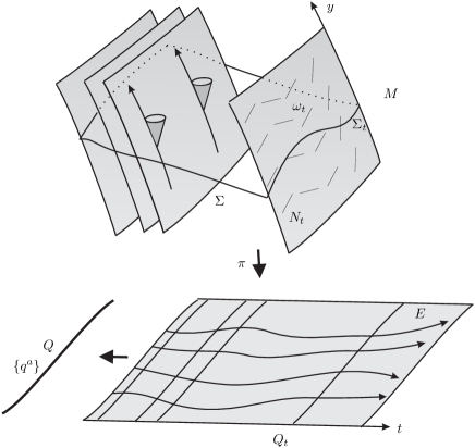
Figure 2: The flow on the base $E$ generates the splitting $E=\mathbb{R}\times Q$. The figure depicts the section $\Sigma:E\to M$, of the fiber bundle $\pi:M\to E$, and its slices $\Sigma_{t}:Q_{t}\to N_{t}$. The 1-forms $\omega_{t}={\rm d}y-b_{t}$ over $N_{t}$ are represented through their kernel.

This discussion clarifies that while the Lagrangian function depends on the choice of coordinates, namely in the way we split the trivial bundles $\pi:M\to E$ and $t:E\to T$, the dynamics, captured in the spacetime lightlike geodesics, is independent of such choice. Therefore, it is natural to investigate whether there are particularly simple choices for those splittings which simplify the dynamics. We shall devote this section to answer to this problem.

3.2.1 Change of gauge

The chosen splitting of the fiber bundle $\pi:M\to E$ will be referred to as a “gauge” and the change of splitting as a “change of gauge”. A change of gauge amounts to a redefinition of the coordinate $y$, namely there is a function $\alpha:\mathbb{E}\to\mathbb{R}$ such that

$$y^{\prime}=y+\alpha(t,q),$$ (32)

whereas the other coordinates are left unchanged: $t^{\prime}=t$, $q^{\prime}=q$. Since our old coordinates of the form $(t,q,y)$ provided a $C^{r+1}$ atlas, the new coordinates of the form $(t,q,y^{\prime})$ provide a $C^{r+1}$ atlas only if $\alpha$ is $C^{r+1}$, otherwise the new atlas is a $C^{k}$ atlas, $k<r+1$, where $k$ is the degree of differentiability of $\alpha$.

Under the above change of section the components of the spacetime metric change as follows

$$a^{\prime}_{t} =a_{t},$$ (33)

$$b_{t}^{\prime} =b_{t}+\partial_{q}\alpha,$$ (34)

$$V^{\prime} =V-\partial_{t}\alpha.$$ (35)

The Lagrangian changes by a ‘total differential’ (as expected, this change does not affect the action and hence the dynamics)

$$L^{\prime}(t,q,v)=L(t,q,v)+[\partial_{q}\alpha(v)+\partial_{t}\alpha]=L+\frac{{\rm d}}{{\rm d}t}\alpha.$$ (36)

The Hamiltonian description changes as follows

$$p^{\prime} =p+\partial_{q}\alpha,$$ (37)

$$H^{\prime}(t,q,p^{\prime}) =H(t,q,p^{\prime}-\partial_{q}\alpha)-\partial_{t}\alpha.$$ (38)

3.2.2 Change of reference frame

Coming to the bundle $\pi:E\to T$, the chosen splitting will be referred to as “reference frame” or “observer” and the change of splitting as a “change of reference frame” or a “change of observer”. We remark that the splitting is induced by a projection $\pi_{Q}:E\to Q$ on a quotient manifold, rather than by a section $\sigma:T\to E$, because $\pi:E\to T$ is not a principal bundle. To change splitting means to change projection $\pi_{Q^{\prime}}:E\to Q^{\prime}$. Of course, $Q$ and $Q^{\prime}$ are diffeomorphic, as for any $t\in T$, $Q$ is diffeomorphic to $Q_{t}$, $Q^{\prime}$ is diffeomorphic to $Q^{\prime}_{t}$ and $Q_{t}=Q^{\prime}_{t}$. On $Q^{\prime}$ we are given coordinate charts $\{q^{k^{\prime}}\}$, and the time dependent coordinate transformation (diffeomorphism) $\nu_{t}:Q^{\prime}\to Q$ can be written

$$q^{\prime}=q^{\prime}(t,q)=\nu_{t}^{-1}(q),$$ (39)

whereas the other coordinates are left unchanged: $y^{\prime}=y$, $t^{\prime}=t$. Let $\hat{v}(t,q)$ be the velocity of the Newtonian flow associated to $Q^{\prime}$ as seen from $Q$. That is, if we write the inverse map as $q=q(t,q^{\prime})=\nu_{t}(q^{\prime})$, then $\hat{v}=\partial q/\partial t$ (this is an element of $TQ$, and by means of the diffeomorphism, it can be regarded as an element $\nu_{t*}^{-1}\hat{v}$ of $TQ^{\prime}$). This change modifies the fields entering the Lagrangian and the spacetime metric as follows

$$a^{\prime}_{t} =\nu_{t}^{*}a_{t},$$

$$b^{\prime}_{t} =\nu_{t}^{*}[b_{t}+a_{t}(\cdot,\hat{v})],$$

$$V^{\prime} =\nu_{t}^{*}[V-\frac{1}{2}a_{t}(\hat{v},\hat{v})].$$

If the diffeomorphism (39) is $C^{k}$, $1\leq k\leq r+1$, then the new fields are $C^{k-1}$. The Lagrangian changes as follows

$$L^{\prime}(t,q^{\prime},v^{\prime})=\nu_{t}^{*}[L(t,q,\nu_{t*}v^{\prime})],$$

and the Hamiltonian description changes as follows

$$p^{\prime} =\nu_{t}^{*}[p+a_{t}(\cdot,\hat{v})],$$

$$H^{\prime}(t,q,p^{\prime}) =\nu_{t}^{*}[H(t,q,\nu_{t}^{-1*}p^{\prime}-a_{t}(\cdot,\hat{v}))-\frac{1}{2}a_{t}(\hat{v},\hat{v})].$$

3.2.3 Geometrization of dynamics through $C^{2}$ solutions of the H.-J. equation

The existence of a solution to the Hamilton-Jacobi equation determines a distinguished section for the bundle $\pi:M\to E$, and the base characteristics provide a flow on $E$ which determines a projection $\pi_{Q}:E\to Q$, and hence a splitting of the bundle $\pi_{T}:E\to T$. In this section we wish to show that we can take advantage of these splittings to simplify the dynamics.

Let us first use the arbitrariness in the choice of gauge.

Theorem 3.11.

Let $u:V\to\mathbb{R}$ be a $C^{k}$, $1\leq k\leq r+1$, solution of the H.-J. equation where $V\supset Q_{t_{0}}$ is an open set with the properties enumerated in theorem 3.7 (there is at least one such neighborhood). Let us redefine $y\to y^{\prime}=y-u(t,q)$, then $a_{t}^{\prime}=a_{t}$ and the new ($C^{k-1}$) Lagrangian takes the Mañe form

$$L^{\prime}(t,q,v)=\frac{1}{2}a_{t}(v+{b^{\prime}}_{t}^{\sharp},v+{b^{\prime}}_{t}^{\sharp}),$$

where ${b^{\prime}}_{t}^{\sharp}=a_{t}^{-1}(\cdot,b^{\prime}_{t})$. The Hamiltonian takes the form

$$H^{\prime}(t,q,p^{\prime})=\frac{1}{2}a_{t}^{-1}(p^{\prime},p^{\prime})-a_{t}^{-1}(p^{\prime},b_{t}^{\prime}).$$

Remark 3.12.

In the $k=1$ case the Lagrangian $L^{\prime}$ is only $C^{0}$ (but smooth in $v$). Nevertheless, the Lagrangian problem makes still sense since $L^{\prime}$ being continuous is integrable, and the dynamics depends on the minimization of the action. One can therefore write the action as usual, express it in terms of the old Lagrangian, and show from there a number of results such as the $C^{r+1}$ nature of the stationary points.

Proof.

We already know that under a change of gauge, $a^{\prime}_{t}=a_{t}$. The change of gauge is $y^{\prime}=y+\alpha(t,q)$ with $\alpha(t,q)=-u(t,q)$. We can rewrite equation (38) as

$$\frac{1}{2}{a}_{t}^{-1}(p^{\prime}-b^{\prime}_{t},p^{\prime}-b^{\prime}_{t})+V^{\prime}(t,q) =H^{\prime}(t,q,p^{\prime})=H(t,q,p^{\prime}+\partial_{q}u)+\partial_{t}u$$

$$=H(t,q,p^{\prime}+\partial_{q}u)-H(t,q,\partial_{q}u).$$

Plugging $p^{\prime}=0$ into the equation we obtain the identity $\frac{1}{2}{a}_{t}^{-1}(b^{\prime}_{t},b^{\prime}_{t})+V^{\prime}=0$. Thus the new Lagrangian is

$$L^{\prime}(t,q,v)=\frac{1}{2}\,a_{t}(v,v)+b^{\prime}_{t}(v)+\frac{1}{2}a_{t}({b^{\prime}}_{t}^{\sharp},{b^{\prime}}_{t}^{\sharp})=\frac{1}{2}a_{t}(v+{b^{\prime}}_{t}^{\sharp},v+{b^{\prime}}_{t}^{\sharp}).$$

Equation (35) shows that $b^{\prime}_{t}$ is $C^{k-1}$ thus $L^{\prime}$ is $C^{k-1}$. The derivation of the Hamiltonian is straightforward. ∎

It must be noted that an Hamiltonian of the form $H^{\prime}$ admits the constant functions as solutions to the Hamilton-Jacobi equation. Indeed, the lightlike hypersurface of equation $y=u(t,q)$, under the change of coordinate, is determined by the new equation $y^{\prime}=0$.

The mentioned lightlike hypersurface is generated by lightlike lines which project into maximal solution to the E.-L. equations. The idea is to use this flow of characteristics as the reference frame. We expect that this choice could simplify the motion of particles ‘moving outside the flow’. This flow could be defined just in the neighborhood of a point $e\in E$ of interest, thus the same is true for the required solution to the H.-J. equation. For simplicity we give the proof of the next theorem in the case in which we have a solution of the H.-J. equation in a time-local sense, that is, defined over a whole connected open interval $I$ of the real line.

Theorem 3.13.

Let $V=[t_{0},t_{1}]\times Q$, and suppose that $u:V\to\mathbb{R}$ is a $C^{k}$, $2\leq k\leq r+1$, solution of the H.-J. equation. Suppose that the base characteristics induced on $V$ by $u$ are defined on the whole interval $[t_{0},t_{1}]$ (this is assured if the E.-L. flow is complete on the interval, which in turn is the case if $Q$ is compact). Identify $Q_{t_{0}}$ with the body frame manifold $Q^{\prime}$ of this (base) characteristic flow $\nu_{t}:Q^{\prime}\to Q$. Then $\nu_{t}:Q^{\prime}\to Q$ is a $C^{k-1}$ diffeomorphism (including the time dependence) and redefined

$$y^{\prime} =y-u(t,q),$$ (40)

$$q^{\prime} =\nu_{t}^{-1}(q),$$ (41)

the Lagrangian in the new variables reads

$$L^{\prime}(t,q^{\prime},v^{\prime})=\frac{1}{2}a^{\prime}_{t}(v^{\prime},v^{\prime}).$$

where $a_{t}^{\prime}$ is $C^{k-2}$. That is, the solutions of the E.-L. equations, as seen from the new frame, appear as geodesics on the new time dependent Riemannian geometry of metric $a^{\prime}_{t}=\nu_{t}^{*}a_{t}$.

Proof.

Let us identify $Q^{\prime}$ with $Q_{t_{0}}$. The characteristics are solutions to the E.-L. equations, pass through every point of $V$, and establish a one to one correspondence between $Q_{t_{0}}$ and $Q_{t}$. Since $Q$ can be identified with any $Q_{t}$, this correspondence is the map $\nu_{t}:Q^{\prime}\to Q$. This is a $C^{k-1}$ flow of equation $\dot{q}=a_{t}^{-1}(\cdot,\partial_{q}u-b_{t})$, thus the map $\nu_{t}$ is $C^{k-1}$ (see [54, Theor.17.19]) and mixed derivatives involving $t$ exist and are continuous up to the $k$th order [41, Chap. 5, Cor. 3.2], that is, both $\nu_{t},\partial_{t}\nu_{t}:Q\to Q^{\prime}$ are $C^{k-1}$. The metric $a^{\prime}_{t}$ is therefore $C^{k-2}$. ∎

According to theorem 3.7, given any event $e_{0}\in E$, $e_{0}=(t_{0},q_{0})$, by choosing a sufficiently smooth initial condition $u_{t_{0}}$ it is indeed possible to find a $C^{2}$ solution $u(t,q)$ of the H.-J. equation which is defined over a neighborhood of $e_{0}$. As a consequence, at any event $e_{0}$ we can observe the motion from the frame given by the characteristics of $u$ to conclude that it locally looks like a geodetic motion in an time dependent geometry.

It must be stressed that, generically, the frame will be local in space unless we can find a time-local (rather than spacetime-local) $C^{2}$ solution to the H.-J. equation, and it will last only a finite time interval because the flow might develop caustics or some characteristic might go to infinity in a finite time (blow up).

3.2.4 Motion in a time dependent geometry

The previous section suggest to study the E.-L. equation for the Lagrangian $L(t,q,v)=\frac{1}{2}a_{t}(v,v)$, that is (see Eq. 31),

$$\frac{D^{t}}{{\rm d}t}\,\dot{q}=-(a_{t}^{-1}\partial_{t}a_{t})(\dot{q}),$$ (42)

where $D^{t}$ is the Levi-Civita connection for $a_{t}$. A special case is that of a uniformly expanding or contracting geometry: $a_{t}=s^{2}(t)a$, where $s(t)>0$ is a scale factor and $a$ is a Riemannian metric. In this case $D^{t}$ is independent of time and coincides with the affine connection for $a$. The equation of motion becomes

$$\frac{D}{{\rm d}t}\dot{q}=-2(\partial_{t}\ln s)\dot{q},$$ (43)

and redefined $\eta=\int_{0}^{t}\frac{{\rm d}r}{s(r)^{2}}+cnst.$, we obtain

$$\frac{D}{{\rm d}\eta}\frac{{\rm d}q}{{\rm d}\eta}=0.$$ (44)

In other words, with respect to the comoving observer, the expansion of geometry can be removed with a redefinition of time. By using a convenient time parameter $\eta$, the motion of neighboring particles which move outside the flow appears as geodesic (this result can also be understood rewriting the spacetime metric as $g=s^{2}(a-\frac{{\rm d}t}{s^{2}}\otimes{\rm d}y-{\rm d}y\otimes\frac{{\rm d}t}{s^{2}})$ and recalling that null geodesics get just reparametrized under conformal changes).

More generally, the right-hand side of Eq. (42) provides the acceleration induced from the dynamics of geometry, and in order to appreciate its effect one can choose coordinates $q$ so at to diagonalize the metric $a_{t}$ at the event $e$ of interest. Once $a_{t}$ is made Euclidean at $e$ one can decompose the matrix $(a_{t}^{-1}\partial_{t}a_{t})$ in its antisymmetric, symmetric and traceless, proportional to the identity, components where the latter represents the expansive term. One can work out the effect of each term. For instance, the antisymmetric part induces a kind of Coriolis force.

3.3 Local and global existence of Rosen coordinates

The subject of this work is the study of the manifold $M=T\times{Q}\times\mathbb{R}$ endowed with the Brinkmann’s (Eisenhart’s) metric

$$g=a_{t}\!-\!{\rm d}t\otimes({\rm d}y-\!b_{t})-\!({\rm d}y-\!b_{t})\otimes{\rm d}t-2V{\rm d}t^{2}.$$ (45)

A well known question is whether this spacetime metric can be rewritten, under a change of variables, in the simplified Rosen form

$$g=a^{\prime}_{t}\!-\!{\rm d}t\otimes{\rm d}y^{\prime}-\!{\rm d}y^{\prime}\otimes{\rm d}t.$$ (46)

where $\partial_{y^{\prime}})_{t,q^{\prime}}$ is still the null Killing field $n=\partial_{y})_{t,q}$. It must be noted that under the assumption $\partial_{y}=\partial_{y^{\prime}}$, the coordinate $t$ does not change because ${\rm d}t=-g(\cdot,\partial_{y})=-g(\cdot,\partial_{y^{\prime}})={\rm d}t^{\prime}$, namely $t$ and $t^{\prime}$ differ by an irrelevant additive constant. We shall speak of Rosen coordinates $(t,q^{\prime},y^{\prime})$, but we do not mean with this terminology that a single coordinate patch suffices to cover $Q$.

A proof that, at least locally, this simplification can indeed be accomplished can be found in [90, Chap. 10], [8], [40, Chap. 4], [19, Sect. 20.5], [84, Sect. 24.5]. These proofs are given under some additional assumptions on the Brinkmann form (four dimensionality, time independence of the space metric, flatness of the space metric, $b_{t}=0$, quadratic dependence of $V(t,q)$ on $q$, etc.). These restriction arise naturally if one imposes the vacuum Einstein equations (which we do not impose). The mentioned proofs are quite technical. As we shall realize in a moment, this transformation problem is in fact quite geometrical although, to appreciate it, the general framework of this paper will be required.

Unfortunately, the fact that such local transformation can hardly be globalized is not so often mentioned. A relevant exception is Penrose [77]. He reminds us that Rosen showed that any non-flat vacuum metric of the form (46) necessarily encounters singularities when one attempts to extend the range of coordinates in order to obtain a geodesically complete spacetime. Unfortunately, Rosen interpreted it as evidence that gravitational plane waves do not exist in general relativity. It was later shown by Robinson [9] that these singularities are due to a mere coordinate effect and that in the four-dimensional case, vacuum metrics admit a global coordinate chart in which they take the form

$$g=\sum_{i=1}^{2}({\rm d}q_{i})^{2}\!-\!{\rm d}t\otimes{\rm d}y-\!{\rm d}y\otimes{\rm d}t-2(\sum_{i=1}^{2}h_{ij}(t)q_{i}q_{j})\,{\rm d}t^{2},$$

that is, they fall into the class of Brinkmann’s metrics studied in this work.

Let us return to our spacetimes $(M,g)$. We are going to show that the possibility of finding local (global) Rosen coordinates is equivalent to the possibility of finding local (resp. global) solutions to the Hamilton-Jacobi equation. The existence of local solutions to the H.-J. equation is then assured by the method of characteristics.

Theorem 3.14.

At any point $p\in M$, the spacetime $(M,g)$ admits ($C^{r-1}$) coordinates in a neighborhood of $p$ which allow us to rewrite $g$ in the Rosen form (46) with a $C^{r-2}$ space metric.

The spacetime $(M,g)$ admits global (time-local at $t=t_{0}$) Rosen coordinates if and only if there is a global (resp. time-local at $t=t_{0}$) solution of the H.-J. equation with Hamiltonian (8) whose base characteristics are complete (resp. defined on a common time interval neighborhood of $t_{0}$). (for the details on the differentiability properties see the proof)

Proof.

Let $p=(t_{0},q^{\prime},y)$. Since the Lagrangian is $C^{r}$, $r\geq 2$, the flow $(t,q^{\prime})\to(t,q(t,q^{\prime}))$ induced by the base characteristics is $C^{r-1}$. We can always choose an initial condition $u_{t_{0}}$, $u_{t_{0}}(q^{\prime})=y$, which is $C^{r}$ and prove that the obtained solution of the H.-J. equation is $C^{r}$ in a neighborhood of $(t,q^{\prime})$. The new coordinate $y^{\prime}=y-u(t,q)$ is therefore $C^{r}$ while the map $q(t,q^{\prime})$ is $C^{r-1}$ together with its (local) inverse $q^{\prime}(t,q)$. The fact that with this change the metric simplifies to the Rosen form follows from the spacetime-local version of theorem 3.13.

As for the last statement, we give the proof in the global case, the time-local case being analogous. Suppose that there are $C^{1}$ coordinates through which the metric can be written in Rosen form for some continuous metric coefficients. The hypersurface $\mathcal{N}$ of equation $y^{\prime}=0$ is $C^{1}$, lightlike and transverse to $\partial_{y^{\prime}})_{t,q^{\prime}}=n$. Let us look at this hypersurface using the original Brinkmann coordinates. According to theorem 3.3 there is a global $C^{1}$ solution of the H.-J. equation whose graph coincides with $\mathcal{N}$. Using again the Rosen form, the base characteristics of this solution are the curves $q^{\prime}=const.$ thus, by assumption, they are defined on the whole time axis.

Conversely, suppose that $u(t,q)$ is a $C^{k}$, $2\leq k\leq r+1$, solution of the H.-J. equation and that the base characteristics are complete. According to theorem 3.13 there are $C^{k-1}$ coordinates $y^{\prime},q^{\prime}$ which bring the metric in Rosen form.

∎

4 The causal hierarchy for spacetimes admitting a parallel null vector

We have already pointed out that the spacetime $(M,g)$ is causal. In this section we wish to establish the position of the generalized gravitational wave spacetime $(M,g)$ in the causal hierarchy of spacetimes [43, 72]. We shall see that, at least for the lower levels, the spacetime is the more causally well behaved the better the continuity properties of the associated least action $S$. The identities $\overline{I^{\pm}(x)}=\overline{J^{\pm}(x)}$, $\overline{I^{+}}=\overline{J^{+}}$, will be used without further mention [43, 72]. Since the causality results depend only on the conformal class of the metric, most of the results of this section will immediately extend to spacetimes which are conformal to those considered here.

A spacetime is non-total imprisoning if no future inextendible causal curve can be contained in a compact set. Replacing future with past gives an equivalent property [3, 66]. Every distinguishing spacetime is non-total imprisoning and every non-total imprisoning spacetime is causal [66].

Theorem 4.1.

The spacetime $(M,g)$ is non-total imprisoning.

Proof.

Suppose, by contradiction, that there is a future (or past) inextendible causal curve contained in a compact set $C$, then, according to [66, Theor. 3.9], there is an inextendible achronal lightlike geodesic $\gamma$ entirely contained in $C$ with the property that, chosen $p\in\gamma$ and $q\in\gamma$ with $q<p$, the portion of $\gamma$ after $p$ accumulates on $q$, in particular $q\in\overline{J^{+}(x)}\backslash\{p\}$. The geodesic $\gamma$ cannot coincide with an integral line of $n$ because $y$ is continuous and would increase along the curve. In the other cases $t$ provides an affine parameter for $\gamma$, it is $t(q)<t(p)$, and since $t$ is continuous and cannot decrease along a causal curve we find again that this case does not apply. The contradiction proves that $(M,g)$ is non-total imprisoning. ∎

Lemma 4.2.

For every $e_{0},e_{1}\in E$ we have

$$\liminf_{e\to e_{1}}\,S(e_{0},e) =S(e_{0},e_{1})\quad\textrm{or}\quad-\infty,$$ (47)

$$\liminf_{e\to e_{0}}\,S(e,e_{1}) =S(e_{0},e_{1})\quad\textrm{or}\quad-\infty,$$ (48)

$$\liminf_{(e,e^{\prime})\to(e_{0},e_{1})}S(e,e^{\prime}) =S(e_{0},e_{1})\quad\textrm{or}\quad-\infty.$$ (49)

Moreover,

$$\overline{J^{+}}=\{(x_{0},x_{1}):y_{1}-y_{0}\geq\liminf_{(e,e^{\prime})\to(e_{0},e_{1})}S(e,e^{\prime})\}.$$ (50)

For every $x_{0}=(e_{0},y_{0})\in M$,

$$\overline{J^{+}(x_{0})} =\{x_{1}:y_{1}-y_{0}\geq\liminf_{e\to e_{1}}S(e_{0},e)\},$$ (51)

$$\overline{J^{-}(x_{1})} =\{x_{0}:y_{1}-y_{0}\geq\liminf_{e\to e_{0}}S(e,e_{1})\}.$$ (52)

Proof.

Proof of Eq. (51), the proof of Eq. (52) being analogous. Let us first prove the inclusion $\{x_{1}:y_{1}-y_{0}\geq\liminf_{e\to e_{1}}S(e_{0},e)\}\subset\overline{J^{+}(x_{0})}$. Let $x_{1}$ be such that $y_{1}\geq y_{0}+\liminf_{e\to e_{1}}S(e_{0},e)$ so that $\liminf_{e\to e_{1}}S(e_{0},e)\neq+\infty$.

There are two cases, either $\liminf_{e\to e_{1}}S(e_{0},e)$ is finite or it is $-\infty$. In the former case let $\epsilon>0$ and let $U\ni e_{1}$ be an open set, then there is $\hat{e}\in U$ such that $S(e_{0},\hat{e})<\liminf_{e\to e_{1}}S(e_{0},e)+\epsilon$. Note that we can assume $S(e_{0},\hat{e})\neq-\infty$ otherwise it would be, from the arbitrariness of $U$, $\liminf_{e\to e_{1}}S(e_{0},e)=-\infty$. Since $\liminf_{e\to e_{1}}S(e_{0},e)\neq+\infty$, we have that $S(e_{0},\hat{e})<+\infty$ and hence $\hat{t}>t_{0}$ or $\hat{e}=e_{0}$. We can assume that we can always choose $\hat{e}\neq e_{0}$ otherwise from the arbitrariness of $U$ and $\epsilon$, $e_{0}=\hat{e}=e_{1}$ and taking the limit of the inequality, $S(e_{0},\hat{e})<\liminf_{e\to e_{1}}S(e_{0},e)+\epsilon$, we get $0=S(e_{0},e_{1})\leq\liminf_{e\to e_{1}}S(e_{0},e)$, thus $y_{1}\geq y_{0}$ and the points $(e_{0},y_{1})$ with $y_{1}\geq y_{0}$ are included in $J^{+}(x_{0})$. Thus let us assume the other case, $\hat{t}>t_{0}$. By Eq. (15) the point $\hat{x}=(\hat{e},y_{1}+\epsilon)$ belongs to $I^{+}(x_{0})$. Since $\epsilon$ and $U$ are arbitrary, $x_{1}\in\overline{I^{+}(x_{0})}=\overline{J^{+}(x_{0})}$.

If $\liminf_{e\to e_{1}}S(e_{0},e)=-\infty$ then there is a sequence $\hat{e}_{n}\to e_{1}$ such that $S(e_{0},\hat{e}_{n})\to-\infty$. Since $S(e_{0},\hat{e}_{n})<+\infty$, $t_{n}>t_{0}$ or $\hat{e}_{n}=e_{0}$. We can assume that the latter possibility does not apply for no value of $n$ because if there were a subsequence $\hat{e}_{k}$ with that property $S(e_{0},\hat{e}_{k})=S(e_{0},{e}_{0})=0$ and could not converge to $-\infty$. By Eq. (15) the points $\hat{x}_{n}=(\hat{e}_{n},y_{1})$ are such that for sufficiently large $n$, $\hat{x}_{n}\in I^{+}(x_{0})$ but $\hat{x}_{n}\to x_{1}$, thus $x_{1}\in\overline{I^{+}(x_{0})}=\overline{J^{+}(x_{0})}$.

For the converse, let $x_{1}\in\overline{J^{+}(x_{0})}=\overline{I^{+}(x_{0})}$. This means that there is a sequence of points $\hat{x}_{n}\in I^{+}(x_{0})$ such that $\hat{x}_{n}\to x_{1}$. By Eq. (15) $\hat{y}_{n}-y_{0}>S(e_{0},\hat{e}_{n})$, and since $\hat{e}_{n}\to e_{1}$, $\liminf_{n\to+\infty}S(e_{0},\hat{e}_{n})\leq y_{1}-y_{0}$ from which the thesis follows.

Proof of Eq. (47), the proof of Eq (48) being analogous. Assume that $\liminf_{e\to e_{1}}S(e_{0},e)<S(e_{0},e_{1})$ (note that it can be $S(e_{0},e_{1})=+\infty$) then, given $y_{0}$, we can choose $y^{\prime}$ such that

$$y_{0}+\liminf_{e\to e_{1}}S(e_{0},e)<y^{\prime}<y_{0}+S(e_{0},e_{1})$$

thus defined $x^{\prime}=(e_{1},y^{\prime})$ and $x_{0}=(e_{0},y_{0})$ we have $x^{\prime}\in\overline{J^{+}(x_{0})}\,\backslash J^{+}(x_{0})$. By the limit curve theorem [4, 65] there is a past inextendible lightlike ray $\eta$ ending at $x^{\prime}$ such that $\eta\subset\overline{J^{+}(x_{0})}$. This null geodesic must belong to the null congruence generated by $n$, otherwise taking $\tilde{y}$ such that

$$y_{0}+\liminf_{e\to e_{1}}S(e_{0},e)<y^{\prime}<\tilde{y}<y_{0}+S(e_{0},e_{1})$$

any point of $\eta\backslash\{x^{\prime}\}$ would be connected to $\tilde{x}=(e_{1},\tilde{y})$ by a timelike curve and thus $\tilde{x}\in I^{+}(x_{0})$, a contradiction with Eq. (15). Since $\eta$ belongs to the congruence and it is past inextendible, every point of the form $(e_{1},y)$ with $y\leq y^{\prime}$ belongs to $\overline{J^{+}(x_{0})}$, and hence from Eq. (51) we get $\liminf_{e\to e_{1}}S(e_{0},e)=-\infty$.

Proof of Eq. (50). Let us first prove the inclusion

$$\{(x_{0},x_{1}):y_{1}-y_{0}\geq\liminf_{(e,e^{\prime})\to(e_{0},e_{1})}S(e,e^{\prime})\}\subset\overline{J^{+}}.$$

Let $x_{0},x_{1}$, be such that $y_{1}\geq y_{0}+\liminf_{(e,e^{\prime})\to(e_{0},e_{1})}S(e,e^{\prime})$ so that

$$\liminf_{(e,e^{\prime})\to(e_{0},e_{1})}S(e,e^{\prime})\neq+\infty.$$

There are two cases, either $\liminf_{(e,e^{\prime})\to(e_{0},e_{1})}S(e,e^{\prime})$ is finite or it is $-\infty$. In the former case let $\epsilon>0$ and let $U,V,$ be open sets such that $U\times V\ni(e_{0},e_{1})$, then there is $(\hat{e},\hat{e}^{\prime})\in U\times V$ such that

$$S(\hat{e},\hat{e}^{\prime})<\liminf_{(e,e^{\prime})\to(e_{0},e_{1})}S(e,e^{\prime})+\epsilon.$$

Note that we can assume $S(\hat{e},\hat{e}^{\prime})\neq-\infty$ otherwise it would be, from the arbitrariness of $U\times V$, $\liminf_{(e,e^{\prime})\to(e_{0},e_{1})}S(e,e^{\prime})=-\infty$. Since

$$\liminf_{(e,e^{\prime})\to(e_{0},e_{1})}S(e,e^{\prime})\neq+\infty,$$

we have that $S(\hat{e},\hat{e}^{\prime})<+\infty$ and hence $\hat{t}^{\prime}>\hat{t}$ or $\hat{e}=\hat{e}^{\prime}$.

We can assume that we can always choose $\hat{e}\neq\hat{e}^{\prime}$ otherwise from the arbitrariness of $U\times V$ and $\epsilon$, $e_{0}=e_{1}$ and $\hat{e}=\hat{e}^{\prime}$ and taking the limit of the inequality, $S(\hat{e},\hat{e}^{\prime})<\liminf_{(e,e^{\prime})\to(e_{0},e_{1})}S(e,e^{\prime})+\epsilon$, we get $0=S(e_{0},e_{1})\leq\liminf_{(e,e^{\prime})\to(e_{0},e_{1})}S(e,e^{\prime})$, thus $y_{1}\geq y_{0}$ and the points $(e_{0},y_{1})$ with $y_{1}\geq y_{0}$ are included in $J^{+}(x_{0})$. Thus let us assume the other case, $\hat{t}>\hat{t}^{\prime}$. By Eq. (15) the points $\hat{x}=(\hat{e},y_{0})$ and $\hat{x}^{\prime}=(\hat{e}^{\prime},y_{1}+\epsilon)$ are chronologically related. Since $\epsilon$ and $U\times V$ are arbitrary, $(x_{0},x_{1})\in\overline{I^{+}}=\overline{J^{+}}$.

If $\liminf_{(e,e^{\prime})\to(e_{0},e_{1})}S(e,e^{\prime})=-\infty$ then there is a sequence $(\hat{e}_{n},\hat{e}^{\prime}_{n})\to(e_{0},e_{1})$ such that $S(\hat{e}_{n},\hat{e}^{\prime}_{n})\to-\infty$. Since $S(\hat{e}_{n},\hat{e}^{\prime}_{n})<+\infty$, we have $t_{n}^{\prime}>t_{n}$ or $\hat{e}_{n}=\hat{e}^{\prime}_{n}$. We can assume that the latter possibility does not apply for no value of $n$ because if there were a subsequence $(\hat{e}_{k},\hat{e}^{\prime}_{k})$ with that property $S(\hat{e}_{k},\hat{e}^{\prime}_{k})=S(\hat{e}_{k},\hat{e}_{k})=0$ and could not converge to $-\infty$. By Eq. (15) the points $\hat{x}_{n}=(\hat{e}_{n},y_{0})$, $\hat{x}_{n}^{\prime}=(\hat{e}_{n},y_{1})$, are such that for sufficiently large $n$, $\hat{x}_{n}^{\prime}\in I^{+}(\hat{x}_{n})$ but $(\hat{x}_{n},\hat{x}_{n}^{\prime})\to(x_{0},x_{1})$, thus $(x_{0},x_{1})\in\overline{I^{+}}=\overline{J^{+}}$.

For the converse, let $(x_{0},x_{1})\in\overline{J^{+}}=\overline{I^{+}}$. This means that there is a sequence of points $(\hat{x}_{n},\hat{x}_{n}^{\prime})\in I^{+}$ such that $(\hat{x}_{n},\hat{x}_{n}^{\prime})\to(x_{0},x_{1})$. By Eq. (15) $\hat{y}^{\prime}_{n}-\hat{y}_{n}>S(\hat{e}_{n},\hat{e}^{\prime}_{n})$, and since $(\hat{e}_{n},\hat{e}_{n}^{\prime})\to(e_{0},e_{1})$, $\liminf_{n\to+\infty}S(\hat{e}_{n},\hat{e}^{\prime}_{n})\leq y_{1}-y_{0}$ from which the thesis follows.

Proof of Eq. (49). Assume that $\liminf_{(e,e^{\prime})\to(e_{0},e_{1})}S(e,e^{\prime})<S(e_{0},e_{1})$ (note that it can be $S(e_{0},e_{1})=+\infty$) then we can choose $\Delta y>0$, $y_{0}$, $y_{1}$, such that

$$\liminf_{(e,e^{\prime})\to(e_{0},e_{1})}S(e,e^{\prime})<y_{1}-y_{0}-\Delta y<y_{1}-y_{0}<S(e_{0},e_{1})$$

thus defined $x=(e_{0},y_{0}+\Delta y/2)$ and $x^{\prime}=(e_{1},y_{1}-\Delta y/2)$ we have $(x,x^{\prime})\in\overline{J^{+}}\,\backslash J^{+}$. By the limit curve theorem [4, 65] there is a future inextendible causal curve $\eta$ starting at $x$ and a past inextendible causal curve $\eta^{\prime}$ ending at $x^{\prime}$ such that for every $w\in\eta$ and $w^{\prime}\in\eta^{\prime}$, $(w,w^{\prime})\in\overline{J^{+}}$. Let us define $x_{0}=(e_{0},y_{0})$ and $x_{1}=(e_{1},y_{1})$. Let us show that either $\eta$ or $\eta^{\prime}$ is a lightlike geodesic generated by $n$. If not there are $w\in\eta\backslash\{x\}$ and $w^{\prime}\in\eta^{\prime}\backslash\{x^{\prime}\}$ such that $(x_{0},w)\in I^{+}$ and $(w^{\prime},x_{1})\in I^{+}$ so that, since $I^{+}$ is open, we have $(x_{0},x_{1})\in I^{+}$ and hence by Eq. (15) $y_{1}-y_{0}>S(x_{0},x_{1})$, a contradiction.

Let us assume that $\eta^{\prime}$ belongs to the congruence generated by $n$, the case of $\eta$ being analogous. Since $\eta^{\prime}$ is past inextendible every point of the form $\tilde{x}=(e_{1},y)$ with $y\leq y_{1}-\Delta y/2$, is such that $(x,\tilde{x})\in\overline{J^{+}}$, thus from Eq. (51) we get $\liminf_{(e,e^{\prime})\to(e_{0},e_{1})}S(e,e^{\prime})=-\infty$.

∎

Lemma 4.3.

If $\liminf_{e\to e_{1}}\,S(e_{0},e)=-\infty$ and $e_{1}^{\prime}$ is such that $t_{1}^{\prime}\geq t_{1}$ then $\liminf_{e\to e_{1}^{\prime}}\,S(e_{0},e)=-\infty$. Under the strict inequality $t_{1}<t_{1}^{\prime}$ we have the stronger conclusion $S(e_{0}^{\prime},e_{1}^{\prime})=-\infty$. Analogously, if $\liminf_{e\to e_{0}}\,S(e,e_{1})=-\infty$ and $e_{0}^{\prime}$ is such that $t_{0}^{\prime}\leq t_{0}$ then $\liminf_{e\to e_{0}^{\prime}}\,S(e,e_{1})=-\infty$. Under the strict inequality $t_{0}^{\prime}<t_{0}$ we have the stronger conclusion $S(e_{0}^{\prime},e_{1}^{\prime})=-\infty$.

Proof.

Let $U\ni e_{1}^{\prime}$ be an open set and let $e\in U$, $t(e)>t_{1}^{\prime}\geq t_{1}$, so that $S(e_{1},e)<+\infty$ and we can find $\Delta y>S(e_{1},e)$ such that for every $y_{1}$, $(e,y_{1}+\Delta y)\in I^{+}((e_{1},y_{1}))$. Since $\liminf_{e\to e_{1}}\,S(e_{0},e)=-\infty$, for every $y_{1}$, $(e_{1},y_{1})\in\overline{J^{+}((e_{0},y_{0}))}$ and hence $(e,y_{1}+\Delta y)\in{I^{+}((e_{0},y_{0}))}$. Since $y_{1}$ is arbitrary, chosen any $r\in\mathbb{R}$, $(e,r)\in{I^{+}((e_{0},y_{0}))}$, and since $U$ is arbitrary, $(e_{1}^{\prime},r)\in\overline{I^{+}((e_{0},y_{0}))}$. From Eq. (51) we get $\liminf_{e\to e_{1}^{\prime}}\,S(e_{0},e)=-\infty$.

If $t_{1}<t_{1}^{\prime}$ then $S(e_{1},e_{1}^{\prime})<+\infty$ and we can find $\Delta y>S(e_{1},e)$. For every $y_{1}$, $(e_{1}^{\prime},y_{1}+\Delta y)\in I^{+}((e_{1},y_{1}))$ but $(e_{1},y_{1})\in\overline{J^{+}((e_{0},y_{0}))}$ thus $(e_{1}^{\prime},y_{1}+\Delta y)\in I^{+}((e_{0},y_{0}))$ and from Eq. (15) and the arbitrariness of $y_{1}$ we get $S(e_{0},e_{1}^{\prime})=-\infty$.

∎

Lemma 4.4.

If $\liminf_{(\check{e},\hat{e})\to(e_{0},e_{1})}\,S(\check{e},\hat{e})=-\infty$ and $(e_{0}^{\prime},e_{1}^{\prime})$ is such that $t_{0}^{\prime}\leq t_{0}$ and $t_{1}\leq t_{1}^{\prime}$ then $\liminf_{(\check{e},\hat{e})\to(e_{0}^{\prime},e_{1}^{\prime})}\,S(\check{e},\hat{e})=-\infty$. Under the strict inequalities $t_{0}^{\prime}<t_{0}$ and $t_{1}<t_{1}^{\prime}$ we have the stronger conclusion $S(e_{0}^{\prime},e_{1}^{\prime})=-\infty$.

Proof.

The assumption $\liminf_{(\check{e},\hat{e})\to(e_{0},e_{1})}\,S(\check{e},\hat{e})=-\infty$ implies that $t_{0}\leq t_{1}$. Let $U,V,$ be open sets, $U\times V\ni(e_{0}^{\prime},e_{1}^{\prime})$ and let $(\hat{e},\check{e})\in U\times V$, such that $t(\check{e})<t_{0}^{\prime}\leq t_{0}$ and $t(\hat{e})>t_{1}^{\prime}\geq t_{1}$, so that $\max(S(\check{e},e_{0}),S(e_{1},\hat{e}))<+\infty$ and we can find $\Delta y>\max(S(\check{e},e_{0}),S(e_{1},\hat{e}))$ so that for every $\check{y},\hat{y}$, $(\check{e},\check{y}-\Delta y)\in I^{-}((e_{0},\check{y}))$ and $(\hat{e},\hat{y}+\Delta y)\in I^{+}((e_{1},\hat{y}))$. Since $\liminf_{({e},{e}^{\prime})\to(e_{0},e_{1})}\,S({e},{e}^{\prime})=-\infty$, for every $\check{y},\hat{y}$, $((e_{0},\check{y}),(e_{1},\hat{y}))\in\overline{J^{+}}$ and hence $((\check{e},\check{y}-\Delta y),(\hat{e},\hat{y}+\Delta y))\in{I^{+}}$. From the arbitrariness of $\check{y}$ and $\hat{y}$ we have that for every $\check{r},\hat{r}\in\mathbb{R}$, $((\check{e},\check{r}),(\hat{e},\hat{r}))\in{I^{+}}$. Since $U\times V$ is arbitrary, $((e_{0}^{\prime},\check{r}),(e_{1}^{\prime},\hat{r}))\in\overline{I^{+}}$ and from Eq. (50) we get the thesis.

For the last statement, since $t_{0}^{\prime}<t_{0}$ and $t_{1}<t_{1}^{\prime}$, we have $e_{0}^{\prime}\neq e_{1}^{\prime}$ and there is a constant $C<+\infty$ such that $S(e_{0}^{\prime},e_{0})<C$ and $S(e_{1},e_{1}^{\prime})<C$. Let $(\check{e}_{n},\hat{e}_{n})\to(e_{0},e_{1})$ be a sequence such that $\lim S(\check{e}_{n},\hat{e}_{n})\to-\infty$. Since $S$ is upper semi-continuous outside the diagonal (corollary 2.9) we can assume $S(e_{0}^{\prime},\check{e}_{n})<C$ and $S(\hat{e}_{n},e_{1}^{\prime})<C$. From the triangle inequality we get

$$S(e_{0}^{\prime},e_{1}^{\prime})\leq S(e_{0}^{\prime},\check{e}_{n})+S(\check{e}_{n},\hat{e}_{n})+S(\hat{e}_{n},e_{1}^{\prime})\leq 2C+S(\check{e}_{n},\hat{e}_{n}),$$

and thus $S(e_{0}^{\prime},e_{1}^{\prime})=-\infty$.

∎

An immediate consequence of lemmas 4.2 and 4.4 is

Proposition 4.5.

If $S(e_{0},e_{1})$ is finite for every $e_{0},e_{1}\in E$ with $t_{0}<t_{1}$ then $S:E\times E\to(-\infty,+\infty]$ is (everywhere) lower semi-continuous.

Proof.

If $S$ were not lower semi-continuous at $e_{0},e_{1}$ then $\liminf_{(\check{e},\hat{e})\to(e_{0},e_{1})}\,S(\check{e},\hat{e})<S(e_{0},e_{1})$ which would imply $t_{0}\leq t_{1}$ and, by lemma 4.2, $\liminf_{(\check{e},\hat{e})\to(e_{0},e_{1})}\,S(\check{e},\hat{e})=-\infty$ and from lemma 4.4 would give for chosen $e_{0}^{\prime},e_{1}^{\prime}$ with $t_{0}^{\prime}<t_{0}$ and $t_{1}<t_{1}^{\prime}$, $S(e_{0}^{\prime},e_{1}^{\prime})=-\infty$, a contradiction. ∎

4.1 Equivalence between stable and strong causality

It is well known that in a generic spacetime the relation $\overline{J^{+}}$ is not transitive. Indeed, the smallest closed and transitive relation which contains $J^{+}$, denoted $K^{+}$ by Sorkin and Woolgar [83], is particularly important. Seifert had also introduced a closed and transitive relation [79], denoted $J^{+}_{S}$, whose antisymmetry is equivalent to stable causality and hence to the existence of a time function [44, 64]. The equivalence between the antisymmetry of $K^{+}$, called $K$-causality, and stable causality has been recently established in [69], and will be central to establish the equivalence between strong causality and stable causality for generalized gravitational wave spacetimes.

Usually, $K^{+}$ does not identify with any simple relation constructed in terms of causal curves, but for causally simple spacetimes and a few other exceptions. Fortunately, in the case of generalized gravitational wave spacetimes considered in this work the next result holds

Theorem 4.6.

On the spacetime $(M,g)$ the relation $\overline{J^{+}}$ is transitive and thus coincident with $K^{+}$.

Proof.

Let $(x_{0},x_{1})\in\overline{J^{+}}$ and $(x_{1},x_{2})\in\overline{J^{+}}$, so that $t_{0}\leq t_{1}\leq t_{2}$.
If $\liminf_{({e},{e}^{\prime})\to(e_{0},e_{1})}\,S({e},{e}^{\prime})$ $=-\infty$ or $\liminf_{({e},{e}^{\prime})\to(e_{1},e_{2})}\,S({e},{e}^{\prime})$ $=-\infty$ then by lemma 4.4, $\liminf_{({e},{e}^{\prime})\to(e_{0},e_{2})}\,S({e},{e}^{\prime})=-\infty$ and hence by Eq. (50), $(x_{0},x_{2})\in\overline{J^{+}}$. If, on the contrary, both liminf are finite then by lemma 4.2 they coincide respectively with $S(e_{0},e_{1})$ and $S(e_{1},e_{2})$ and hence

$$y_{1}-y_{0} \geq S(e_{0},e_{1}),$$

$$y_{2}-y_{1} \geq S(e_{1},e_{2}),$$

which, using the triangle inequality for $S$ give

$$y_{2}-y_{0}\geq S(e_{0},e_{1})+S(e_{1},e_{2})\geq S(e_{0},e_{2}),$$

and hence by Eq. (50), $(x_{0},x_{2})\in\overline{J^{+}}$. ∎

The previous result simplifies considerably the causal ladder for generalized gravitational wave spacetimes. A strongly causal spacetime for which $\overline{J^{+}}$ is transitive is called causally easy. It has been proved [69] that causal continuity implies causal easiness which implies stable causality. Thus the previous theorem implies

Theorem 4.7.

For the generalized gravitational wave spacetime $(M,g)$, strong causality and stable causality are equivalent (they are actually equivalent to causal easiness).

This result implies that the infinite causality levels that one may construct between strong causality and stable causality are actually all coincident for this type of spacetime.

It is therefore interesting to establish under which conditions strong causality holds.

Theorem 4.8.

The spacetime $(M,g)$ is strongly causal at an event $x$ iff it is strongly causal at every other event $y$ on the same time slice (i.e. $t(y)=t(x)$) iff $S:E\times E\to[-\infty,+\infty]$ is lower semi-continuous at $(e_{x},e_{x})$. In particular strong causality holds iff $S$ is lower semi-continuous on the diagonal $\{(e,e):e\in E\}$.

Proof.

Assume that for some event $x$, $\liminf_{(e,e^{\prime})\to(e_{x},e_{x})}S(e,e^{\prime})=-\infty$ and let $y$ be an event such that $t(y)=t(x)$. By lemma 4.4

$$\liminf_{(e,e^{\prime})\to(e_{y},e_{x})}S(e,e^{\prime})=\liminf_{(e,e^{\prime})\to(e_{x},e_{y})}S(e,e^{\prime})=\liminf_{(e,e^{\prime})\to(e_{y},e_{y})}S(e,e^{\prime})=-\infty.$$

Strong causality is violated at $p$ iff there is a point $q\in J^{-}(p)$, $q\neq p$, such that $(p,q)\in\overline{J^{+}}$ (see [76, Lemma 4.16] or the proof of [63, theorem 3.4]).

By lemmas 4.2 and 4.4, strong causality is violated at $x$ if and only if $\liminf_{(e,e^{\prime})\to(e_{x},e_{x})}S(e,e^{\prime})=-\infty$ (which, by Eq. (49), holds iff $S$ is not lower semi-continuous at $e_{x}$). Indeed, if the latter equality holds then $w=(e_{x},y_{x}-1)$ is such that $(w,x)\in J^{+}$, $w\neq x$ and $(x,w)\in\overline{J^{+}}$. Conversely, if there is some $w$ with these properties then as $(w,x)\in J^{+}$, $t_{w}\leq t_{x}$, and since $(x,w)\in\overline{J^{+}}$ and $t$ is continuous, $t_{x}\leq t_{w}$, so that they stay in the same time slice. Using again $(w,x)\in J^{+}$ it follows that $w$ stays in the past lightlike ray generated by $n$ that ends at $x$, so that $e_{w}=e_{x}$. Thus $(x,w)\in\overline{J^{+}}$, $w\neq x$, and Eq. (50) together with $S(e_{x},e_{x})=0$ implies that $\liminf_{(e,e^{\prime})\to(e_{x},e_{x})}S(e,e^{\prime})=-\infty$. ∎

4.2 Distinguishing spacetimes

Let us recall [52, 67] that a spacetime is future distinguishing if $I^{+}(x)=I^{+}(y)\Rightarrow x=y$; past distinguishing if $I^{-}(x)=I^{-}(y)\Rightarrow x=y$; and weakly distinguishing if ‘$I^{+}(x)=I^{+}(y)$ and $I^{-}(x)=I^{-}(y)$’$\Rightarrow x=y$. The spacetime is distinguishing if it is both future and past distinguishing, namely if ‘$I^{+}(x)=I^{+}(y)$ or $I^{-}(x)=I^{-}(y)$’$\Rightarrow x=y$. Another useful characterization of future distinction is the fact that at the point $x$ there are arbitrarily small neighborhoods such that no causal curve issued from $x$ can escape and later reenter the neighborhood [43, 72]. Similar characterizations hold for past distinction and distinction (but not for weak distinction).

There are other useful characterizations. Let us recall that the relations $D^{+}_{f}=\{(x,y):y\in\overline{I^{+}(x)}\}$, $D^{+}_{p}=\{(x,y):x\in\overline{I^{-}(x)}\}$, and $D^{+}=D^{+}_{f}\cap D^{+}_{p}$ are transitive [63]. Moreover, $D^{+}_{f}$ ($D^{+}_{p}$) is antisymmetric iff the spacetime is future (resp. past) distinguishing, and $D$ is antisymmetric iff the spacetime is weakly distinguishing [63].

It is clear from lemma 2.1 that the chronological relation is determined by the least action $S$. The conformal structure follows also from the chronological relation and hence from $S$ provided the spacetime is distinguishing (Malament’s theorem [57], see [72, Prop. 3.13]). It is possible to completely characterize the distinction of the spacetime $(M,g)$ using the function $S$.

Theorem 4.9.

The spacetime $(M,g)$ is future (resp. past) distinguishing at $x=(e_{1},y_{1})$ iff $S(e_{1},\cdot)$ (resp. $S(\cdot,e_{1})$) is lower semi-continuous at $e_{1}$.

Proof.

Assume $(M,g)$ is not future distinguishing at $x=(t_{x},q_{x},y_{x})$. Then there is $z=(t_{z},q_{z},y_{z})$ such that $I^{+}(x)=I^{+}(z)$ which implies $t_{x}=t_{z}$ because $t$ is a semi-time function. The violation of future distinction implies the existence of a sequence of timelike curves $\tilde{\gamma}_{n}$ of endpoints $x$ and $x_{n}$ such that $x_{n}\to x$, and $z$ is an accumulation point for $\tilde{\gamma}_{n}$. By the limit curve theorem [4, 65], since the spacetime is chronological, there is a lightlike past ray ending at $x$ entirely contained in $\overline{I^{+}(x)}$. Necessarily this lightlike ray $r$ coincides with the portion of the fiber passing through $x$ which stays in the causal past of $x$. Indeed, if it were different, as $-g(n,r^{\prime})={\rm d}t[r^{\prime}]$ is a positive constant, $t$ would be an affine parameter for $r$ and thus $r$ would contain points with $t<t_{x}$ which is impossible since no points of this kind can be contained in $\overline{I^{+}(x)}$. From Eq. (51) we get

$$\liminf_{e\to e_{x}}S(e_{x},e)=-\infty,$$

which violates lower semi-continuity as $S(e_{x},e_{x})=0$.

Conversely, assume $S(e_{x},\cdot)$ is not lower semi-continuous at $e_{x}$, then from lemma 4.2 it follows that the whole past lightlike ray $\eta$ generated by $n$ and ending at $x$ is contained in $\overline{J^{+}(x)}$. Take $w\in\eta\backslash\{x\}$ then as $(w,x)\in J^{+}$ and $w\in\overline{J^{+}(x)}$ we have $I^{+}(x)=I^{+}(w)$, so that future distinction is violated at $x$. ∎

4.3 Reflectivity, causal continuity and independence of time

A spacetime is future reflective if $x\in\overline{I^{-}(y)}\Rightarrow y\in\overline{I^{+}(x)}$, past reflective if $x\in\overline{I^{-}(y)}\Leftarrow y\in\overline{I^{+}(x)}$ and reflective if it is both past and future reflective.

Equivalently [63], future reflectivity reads $D^{+}_{f}=\overline{J^{+}}$ and past reflectivity reads $D^{+}_{p}=\overline{J^{+}}$.

From Eqs. (51) and (52) we get

Theorem 4.10.

The spacetime $(M,g)$ is future reflective iff for every $e_{0},e_{1}\in E$

$$\liminf_{e\to e_{1}}S(e_{0},e)\leq\liminf_{e\to e_{0}}S(e,e_{1}),$$ (53)

and past reflective iff for every $e_{0},e_{1}\in E$

$$\liminf_{e\to e_{1}}S(e_{0},e)\geq\liminf_{e\to e_{0}}S(e,e_{1}).$$ (54)

Moreover, in the former case

$$\liminf_{e\to e_{1}}S(e_{0},e)=\liminf_{(e,e^{\prime})\to(e_{0},e_{1})}S(e,e^{\prime}),$$ (55)

while in the latter case

$$\liminf_{e\to e_{0}}S(e,e_{1})=\liminf_{(e,e^{\prime})\to(e_{0},e_{1})}S(e,e^{\prime}).$$ (56)

An important case is that of autonomous Lagrangians

Theorem 4.11.

If the Lagrangian $L(t,q,v)$ does not depend on time then the spacetime $(M,g)$ is reflective.

Proof.

Let $x_{1}\in\overline{I^{+}(x_{0})}$, $x_{1}=(t_{1},q_{1},y_{1})$, and make a coordinate change change $y^{\prime}=y+Ct$, $t^{\prime}=t$, so that $\partial_{t})_{y^{\prime}}=\partial_{t})_{y}-C\partial_{y}$. From Eq. (3) it follows that this operation changes the Lagrangian by a constant and thus keeps it independent of time. With $C=V(q_{1})-1/2$, $\partial_{t})_{y^{\prime}}$ is timelike at $x_{1}$. For this reason with no loss of generality we can assume that $\partial_{t}$ is timelike at $x_{1}$. The sequence $w_{n}=(\tau_{n},q_{1},y_{1})$ with $\tau_{n}>t_{1}$ and $\tau_{n}\to t_{1}$ stays in the integral line of $\partial_{t}$ passing through $x_{1}$, thus as $\partial_{t}$ is timelike in a neighborhood of $x_{1}$, $w_{n}\in I^{+}(x_{1})$ and hence $w_{m}\in I^{+}(x_{0})$. Let $\sigma_{n}=(t,q_{n}(t),y_{n}(t))$, $w_{n}=\sigma_{n}(\tau_{n})$, $y_{n}(\tau_{n})=y_{1}$, $q_{n}(\tau_{n})=q_{1}$, $\sigma_{n}:[t_{0},\tau_{n}]\to M$ be a sequence of timelike curves starting from $x_{0}$ of final endpoints $w_{n}$. Consider the curves $\tilde{\sigma}_{n}(t)=(t,q_{n}(t-t_{1}+\tau_{n}),y_{n}(t-t_{1}+\tau_{n}))$, $\sigma:[t_{0}+t_{1}-\tau_{n},t_{1}]\to M$ which are obtained translating $\sigma_{n}$ backward under the flow of $\partial_{t}$ by a parameter $\tau_{n}-t_{1}$. By construction the curves $\tilde{\sigma}_{n}$ end at $x_{1}$ and start at $(t_{0}+t_{1}-\tau_{n},q_{0},y_{0})$ which converges to $x_{0}$ for $\tau_{n}\to t_{1}$. Finally, $\tilde{\sigma}_{n}$ is timelike because the causal character of a vector is preserved under the action of the flow of a Killing field, and in our case $\partial_{t}$ is Killing. We conclude that $x_{0}\in\overline{I^{-}(x_{1})}$ and hence past reflectivity holds. The proof of the other direction is analogous. ∎

A theorem by Clarke and Joshi [14, Prop. 3.1] states that every spacetime admitting a complete timelike Killing vector field is reflective. Their theorem is in a way connected to the above result. Indeed, one could hope to prove theorem 4.11 by showing that under independence of time for $L$ the spacetime $(M,g)$ admits a complete timelike Killing vector field. This alternative strategy seems to work only in particular cases. In fact note that while, under time independence, the vector $\partial_{t}+k\partial_{y}$ is complete and Killing for any constant $k$, it is not necessarily globally timelike (although it can be made timelike at some event for some $k$) unless the potential is bounded from below [61, Theor. 2.8].

A spacetime which is distinguishing and reflective is called causally continuous. From theorems 4.9 and 4.10 we obtain

Theorem 4.12.

The spacetime $(M,g)$ is causally continuous iff

$$\liminf_{e\to e_{1}}S(e_{0},e)=\liminf_{e\to e_{0}}S(e,e_{1}),$$ (57)

and this quantity vanishes for $e_{0}=e_{1}$.

Remark 4.13.

Since under Eq. (57) the Eq. (55) holds, then $S$, under the assumptions of theorem 4.12, is lower semi-continuous on the diagonal, which is equivalent to stable causality. This fact is consistent with the well known result that causal continuity implies stable causality.

Corollary 4.14.

If $S:E\times E\to[-\infty,+\infty]$ is lower semi-continuous then $(M,g)$ is causally continuous.

Proof.

If $S$ is lower semi-continuous then

$$\liminf_{e\to e_{1}}S(e_{0},e)=S(e_{0},e_{1})=\liminf_{e\to e_{0}}S(e,e_{1}),$$

and this quantity vanishes for $e_{0}=e_{1}$, because by definition $S(e,e)=0$. ∎

Under reflectivity it is especially important to establish if a spacetime is distinguishing as this property would imply causal continuity. Fortunately, the next proposition shows that it is necessarily to check for distinction at just one point for every time slice (as it happens for strong causality, see theorem 4.8).

Proposition 4.15.

Assume the spacetime $(M,g)$ is reflective. If $(M,g)$ is past or future distinguishing at an event $x$ then it is past and future distinguishing at every other event $y$ on the same time slice (i.e. $t(y)=t(x)$). Moreover, if this is not the case then the events in the time slice have the same chronological past and the same chronological future.

Proof.

Assume that future distinction is violated at $x$ and let us prove that past distinction is violated at $y$ with $t(y)=t(x)$. The violation of future distinction at $x$ implies (see lemma 4.2 and theorem 4.9)

$$\liminf_{e\to e_{x}}S(e_{x},e)=-\infty,$$

thus by lemma 4.3

$$\liminf_{e\to e_{y}}S(e_{x},e)=-\infty,$$ (58)

and using past reflectivity, that is Eq. (54),

$$\liminf_{e\to e_{x}}S(e,e_{y})=-\infty,$$ (59)

and using again lemma 4.3

$$\liminf_{e\to e_{y}}S(e,e_{y})=-\infty,$$

which from lemma 4.2 and theorem 4.9 implies that past distinction is violated at $y$. Analogously, if past distinction is violated at $x$ then future distinction is violated at $y$. As $y$ is arbitrary and can be taken equal to $x$, future distinction is violated at a point iff past distinction is violated at the point, from which the first statement follows. As for the last statement, the previous analysis shows that if future or past distinction is violated at a point then future distinction is violated at $x$, and Eqs. (58) and (59) imply (i) $y\in\overline{J^{+}(x)}$ and (ii) $x\in\overline{J^{-}(y)}$. The analogous omitted part of proof gives (a) $y\in\overline{J^{-}(x)}$ and (b) $x\in\overline{J^{+}(y)}$ from (i) and (b) we get $I^{+}(y)=I^{+}(x)$ and from (ii) and (a) we get $I^{-}(x)=I^{-}(y)$. ∎

Corollary 4.16.

In the time independent case if past or future distinction holds at a point then distinction holds at every point.

Proof.

If past or future distinction holds at $x$ then it holds on the whole time slice passing through $x$. As $\partial_{t}$ is Killing (not necessarily timelike) every event is obtained from a point on the time slice of $x$ by applying the the flow $\phi_{s}$ of the Killing field $\partial_{t}$. As the maps $\phi_{s}$ are isometries one gets the thesis. ∎

4.4 A partially time-independent case: subquadratic potentials

In this subsection we investigate the special case $\partial_{t}a_{t}=b_{t}=0$, and obtain some useful result which improve those obtained in [32]. Further result will be given in the next sections, e.g. Theor. 4.23 and Cor. 4.29. The assumption $\partial_{t}a_{t}=b_{t}=0$ will be explicitly stated wherever it is used.

Definition 4.17.

We shall say that the functional $\mathcal{S}_{e_{0},e_{1}}$ is coercive at $(e_{0},e_{1})$ if given any sequence of $C^{1}$ curves $q_{n}:[t_{0},t_{1}]\to Q$ such that $\mathcal{S}_{e_{0},e_{1}}[q_{n}]$ is bounded from above, the images $q_{n}([t_{0},t_{1}])$ are all contained in a compact subset of $Q$. We shall say that the functional $\mathcal{S}_{e_{0},e_{1}}$ is coercive at if it is coercive everywhere on $E\times E$.

Definition 4.18.

Let $I$ be an interval of the real line, and let $(Q,a)$ be a Riemannian space. A potential $V(t,q)$ defined over $I\times Q$ is said to be

almost quadratic if $$V(t,q) \leq c_{1}D(q_{B},q)^{2}+c_{2},$$

subquadratic if $$V(t,q) \leq c_{1}\,o(D(q_{B},q)^{2})+c_{2},$$

superquadratic if $$V(t,q) \geq c_{1}\omega(D(q_{B},q)^{2})+c_{2},$$

where $q_{B}\in Q$, $c_{1},c_{2}$, are positive constants, and $D(q_{0},q)$ is the Riemannian distance calculated through $a$.

Clearly if $Q$ and $I$ are compact then $V$ is almost quadratic, and it cannot be neither subquadratic nor superquadratic.

It is understood that the little-$o$ and little-$\omega$ Landau notation used above refers to the limit $(t,q)\to+\infty$ on $\mathbb{R}\times Q$, with the Alexandrov one-point compactification topology for the point $+\infty$ (its open sets are the complements to compact sets). In particular, since $D$ is continuous, for fixed $q_{B}$, $D(q_{B},q)\to+\infty$ implies $q\to+\infty$, but the converse holds if and only if $(Q,a)$ is complete (Hopf-Rinow theorem).

Remark 4.19.

The reference point $q_{B}$ can be chosen arbitrarily because, if $q^{\prime}_{B},q_{B}^{\prime\prime}\in Q$ are any two points

$$c_{1}^{\prime}D(q_{B}^{\prime},q)^{2}+c_{2}^{\prime}\leq c_{1}^{\prime}[D(q_{B}^{\prime},q_{B}^{\prime\prime})+D(q_{B}^{\prime\prime},q)]^{2}+c^{\prime}_{2}\leq c_{1}^{\prime\prime}D(q_{B}^{\prime\prime},q)^{2}+c_{2}^{\prime\prime},$$

where $c_{1}^{\prime\prime}=c_{1}^{\prime}+{c_{1}^{\prime}}^{2}$ and $c_{2}^{\prime\prime}=c_{2}^{\prime}+2D(q_{B}^{\prime},q_{B}^{\prime\prime})^{2}$.

The next result allows us to establish the lower semi-continuity of the least action, and hence to infer strong causality. According to a previous result this fact implies stable causality. The theorem rephrases and improves some results contained in [32] where the key role of the quadraticity of the potential was recognized.

Theorem 4.20.

Let us consider the special case $\partial_{t}a_{t}=b_{t}=0$. Suppose that for some compact time interval $I$ the potential $V(t,q)$ on $I\times Q$ is

• Almost quadratic. There is a constant $\epsilon>0$ such that the least action $S({e_{0},e_{1}})$, is finite on $(I\times Q)^{2}$ provided $t_{0}<t_{1}<t_{1}+\epsilon$ (as a consequence $S$ is lower semi-continuous on the diagonal on $(I\times Q)^{2}$, see Theor. 4.5). Moreover, under the same conditions on $t_{1}$, if $(Q,a)$ is complete then $\mathcal{S}_{e_{0},e_{1}}$ is coercive.

• Subquadratic. Same as (a) but we can take $\epsilon=+\infty$.

• Superquadratic. Let $\tilde{e}\in I\times Q$ be such that $\tilde{t}\in\textrm{Int}\,I$. Then $S(\tilde{e},\cdot)$ and $S(\cdot,\tilde{e})$ are not lower semi-continuous at $\tilde{e}$.

Proof.

Let $(e_{0},e_{1})\in(I\times Q)^{2}$ with $t_{0}<t_{1}$, and let us set $q_{B}=q_{0}$. Let $q:[t_{0},t_{1}]\to Q$ be a $C^{1}$ curve connecting $q_{0}$ to $q_{1}$, and let $\tilde{q}$ be a point on the image of $q(t)$ with maximum distance from $q_{B}$ (we recall that the Riemannian distance is continuous). For any given path (image of $q(t)$) the kinetic energy is minimized by that reparametrization which makes the speed constant (Cauchy-Schwarz inequality). As a consequence, the kinetic energy satisfies the lower bound

$$T[q] =\int_{t_{0}}^{t_{1}}\frac{1}{2}a(\dot{q},\dot{q}){\rm d}t\geq\frac{1}{2}\frac{l[q]^{2}}{t_{1}-t_{0}}\geq\frac{1}{2}\frac{[D(q_{0},\tilde{q})+D(\tilde{q},q_{1})]^{2}}{t_{1}-t_{0}}$$

$$\geq\frac{[2D(q_{B},\tilde{q})-D(q_{0},q_{1})]^{2}}{t_{1}-t_{0}},$$

where $l[q]$ is the Riemannian length of the path.

Proof of (a). For an almost quadratic potential we get

$$\mathcal{S}_{e_{0},e_{1}}[q] \geq T[q]-\int_{t_{0}}^{t_{1}}V(t,q(t)){\rm d}t\,\geq T[q]-\int_{t_{0}}^{t_{1}}[c_{1}D(q_{B},q(t))^{2}+c_{2}]{\rm d}t$$

$$\geq T[q]-\int_{t_{0}}^{t_{1}}[c_{1}D(q_{B},\tilde{q})^{2}+c_{2}]{\rm d}t$$

$$\geq\frac{[2D(q_{B},\tilde{q})-D(q_{0},q_{1})]^{2}}{t_{1}-t_{0}}-[c_{1}D(q_{B},\tilde{q})^{2}+c_{2}](t_{1}-t_{0}).$$

If $t_{1}<t_{0}+\epsilon$ with $\epsilon<2/\sqrt{c_{1}}$ then the right-hand side is bounded from below by a constant independent of $\tilde{q}$ and hence of $q(t)$. Taking the infimum over all paths connecting $q_{0}$ to $q_{1}$ we obtain that $S(e_{0},e_{1})\neq-\infty$. Suppose $(Q,a)$ is complete and let us make the same choice for $\epsilon$. The last inequality proves that if $\mathcal{S}_{e_{0},e_{1}}[q]<C$ for some constant $R$, then $D(q_{B},\tilde{q})<R(C,t_{0},t_{1},c_{1},c_{2})$, where the constant in the last equation does not depend on the curve $q(t)$. Thus, as for every $t$, $D(q_{B},q(t))\leq D(q_{B},\tilde{q})$, all connecting curves are contained in a ball of radius $R$, which is compact by the Hopf-Rinow theorem.

Proof of (b). Suppose that the potential is subquadratic. Let us observe that for each $\delta>0$ there is some compact set $K\subset Q$ such that $V(t,q)\leq\delta c_{1}D(q_{B},{q})^{2}+c_{2}$ for $(t,q)\in I\times(Q\backslash K)$. Since over the compact $I\times K$ the potential $V(t,q)$ attains a maximum, there is a constant $c_{2}^{\prime}(\delta)$ such that $V(t,q)\leq\delta c_{1}D(q_{B},{q})^{2}+c_{2}^{\prime}(\delta)$. Thus

$$\mathcal{S}_{e_{0},e_{1}}[q] \geq T[q]-\int_{t_{0}}^{t_{1}}V(t,q(t)){\rm d}t\,\geq T[q]-\int_{t_{0}}^{t_{1}}[\delta c_{1}D(q_{B},q(t))^{2}+c_{2}^{\prime}(\delta)]{\rm d}t$$

$$\geq T[q]-\int_{t_{0}}^{t_{1}}[\delta c_{1}D(q_{B},\tilde{q})^{2}+c_{2}^{\prime}(\delta)]{\rm d}t$$

$$\geq\frac{[2D(q_{B},\tilde{q})-D(q_{0},q_{1})]^{2}}{t_{1}-t_{0}}-[\delta c_{1}D(q_{B},\tilde{q})^{2}+c_{2}^{\prime}(\delta)](t_{1}-t_{0}).$$

Choosing $\delta<\frac{4}{(t_{1}-t_{0})^{2}c_{1}}$ we obtain that the right-hand side is bounded from below by a constant independent of $\tilde{q}$ and hence of $q(t)$. Taking the infimum over all paths connecting $q_{0}$ to $q_{1}$ we obtain that $S(e_{0},e_{1})\neq-\infty$. Arguing as in (a) we also obtain that $\mathcal{S}_{e_{0},e_{1}}[q]$ is coercive.

Proof of (c). Since the potential is superquadratic $Q$ is non compact. Let $q_{B}\in Q$ be any point, even if $(Q,a)$ is not complete there is a small compact ball $B$ of radius $r$ centered at $q_{B}$. Let us define $t_{0}\in\textrm{Int}I$, $e_{0}=(t_{0},q_{B})$, $e_{1}=(t_{0}+3\epsilon,q_{B})$ and let $\epsilon>0$. We wish to prove that $S(e_{0},e_{1}(\epsilon))$ goes to $-\infty$ for $\epsilon\to 0$ (and hence $e_{1}\to e_{0}$), thus proving that $S(e_{0},\cdot)$ is not lower semi-continuous, the proof to the dual claim being analogous.

Let us observe that for each $\delta$, such that $0<\delta<c_{1}\epsilon^{2}/2$ there is some compact set $K\subset Q$, $q_{B}\in K$, such that $V(t,q)\geq\frac{1}{\delta}c_{1}D(q_{B},{q})^{2}+c_{2}$ for $(t,q)\in I\times(Q\backslash K)$. Let $C$ be a lower bound for $V(t,q)$ on the compact set $I\times K$, then $F:=\textrm{min}(C,c_{2})$ is a lower bound for $V(t,q)$ all over $I\times Q$. Let us consider a curve $q:[t_{0},t_{0}+3\epsilon]\to Q$ such that for $t\in[t_{0},t_{0}+\epsilon]$ the point $q(t)$ starts from $q_{B}$, moves at constant speed till it reaches a point $\hat{q}\notin K$, there it stays at rest during the interval $[t_{0}+\epsilon,t_{0}+2\epsilon]$, and then it returns to $q_{B}$ at constant speed along the initial path. Thus

$$S(e_{0},e_{1}) \leq\mathcal{S}_{e_{0},e_{1}}[q]\leq T[q]-\int_{t_{0}}^{t_{0}+3\epsilon}V(t,q(t)){\rm d}t\,$$

$$\leq\frac{D(q_{B},\hat{q})^{2}}{\epsilon}-\int_{t_{0}+\epsilon}^{t_{0}+2\epsilon}[\frac{1}{\delta}c_{1}D(q_{B},q(t))^{2}+c_{2}]{\rm d}t-2\epsilon F$$

$$\leq\frac{D(q_{B},\hat{q})^{2}}{\epsilon}-\epsilon[\frac{1}{\delta}c_{1}D(q_{B},\hat{q})^{2}+c_{2}]-2\epsilon F$$

$$\leq-\frac{D(q_{B},\hat{q})^{2}}{\epsilon}-\epsilon(c_{2}+2F)\leq-\frac{r^{2}}{\epsilon}-\epsilon(c_{2}+2F).$$

This inequality proves that $S(e_{0},e_{1}(\epsilon))\to-\infty$ for $\epsilon\to 0$. ∎

Corollary 4.21.

In the special case $\partial_{t}a_{t}=b_{t}=0$, if the potential $V(t,q)=$ is almost quadratic then the spacetime is stably causal.

Remark 4.22.

We stress that the previous result for the small family of gravitational plane waves was already known. In fact Ehrlich and Emch proved that for $Q=\mathbb{R}^{2}$, $a_{ij}=\delta_{ij}$, $V(t,q)=f(t)(w^{2}-z^{2})+g(t)wz$ the spacetime is even causally continuous [23, Theor. 6.9]. Similarly, Hubeny, Rangamani and Ross [47] showed that if $Q=\mathbb{R}^{d}$, $a_{ij}=\delta_{ij}$, $V(t,q)=A_{ij}(t)x^{i}x^{j}$, then the spacetime is stably causal. Contrary to these references we do not assume any symmetry, nor an exact quadratic dependence. These last authors claim [47] that a proof of the above corollary can be found in [32], but in this paper the authors do not mention stable causality, and prove just strong causality. In fact, we have seen that the above result depends on the recently proved equivalence between $K$-causality and stable casuality [69, 70].

The following result improves [32, Prop. 2.1], because our superquadraticity condition is less restrictive, the Riemannian manifold $(Q,a)$ is not assumed complete, and $V(t,q)$ is not necessarily non-negative.

Theorem 4.23.

Let us consider the special case $\partial_{t}a_{t}=b_{t}=0$. If $V(t,q)$ is superquadratic for every $t\in I$, with $I\subset\mathbb{R}$ open interval, then $(M,g)$ is not distinguishing on any point of $\pi^{-1}(I\times Q)$.

Proof.

It follows from Theorem 4.20 and Theorem 4.9. ∎

4.5 Global hyperbolicity and causal simplicity: from coercivity to Tonelli’s theorem

A spacetime is causally simple if it is causal and $\overline{J^{+}}=J^{+}$ (see [72]). The level of causal simplicity has been characterized by the author in [61]. Here I provide a shorter proof of the following theorem taking advantage of the previous results.

Theorem 4.24.

The spacetime $(M,g)$ is causally simple iff the following properties hold

• if $S(e_{0},e_{1})$, $t_{0}<t_{1}$, is finite then the functional $\mathcal{S}_{e_{0},e_{1}}$ attains its infimum at a certain (non necessarily unique) ${q}(t)\in C^{1}_{e_{0},e_{1}}$, i.e. $\mathcal{S}_{e_{0},e_{1}}[{q}]=S(e_{0},e_{1})$,

• $S$ is lower semi-continuous.

Proof.

From Eq. (16) and (50) we have

$$\overline{J^{+}}\backslash J^{+}\supset\{(x_{0},x_{1}):\liminf_{(e,e^{\prime})\to(e_{0},e_{1})}S(e,e^{\prime})\leq y_{1}-y_{0}<S(e_{0},e_{1})\},$$

thus causal simplicity implies (b). Assume $S(e_{0},e_{1})$, $t_{0}<t_{1}$, is finite and for any $y_{0}$ define $x_{0}=(e_{0},y_{0})$ and $x_{1}=(e_{1},y_{0}+S(e_{0},e_{1}))$. By Eq. (50), $(x_{0},x_{1})\in\overline{J^{+}}=J^{+}$. However, from Eq. (15) we infer $x_{1}\notin I^{+}(x_{0})$ thus $x_{1}\in E^{+}(x_{0})$ and there is an achronal lightlike geodesic $\gamma$ connecting $x_{0}$ to $x_{1}$ necessarily (because $t_{1}>t_{0}$) with tangent vector nowhere parallel to $n$. Let $(t,q(t))$ be the $C^{1}$ curve projection of the geodesic $\gamma$ on $E$. By corollary 2.8, $\mathcal{S}_{e_{0},e_{1}}[q]=S(e_{0},e_{1})$ thus (a) holds.

For the converse, since by (b) $S$ is lower semi-continuous, Eq. (50) gives

$$\overline{J^{+}}=\{(x_{0},x_{1}):y_{1}-y_{0}\geq S(e_{0},e_{1})\}.$$

Given $(x_{0},x_{1})\in\overline{J^{+}}$ we have by the previous equation, $S(e_{0},e_{1})<+\infty$, thus either $e_{0}=e_{1}$ and hence $(x_{0},x_{1})\in J^{+}$ and we have finished, or $t_{0}<t_{1}$. In this last case by (a) there is some $C^{1}$ curve $(t,q(t))$ which connects $e_{0}$ to $e_{1}$ and such that $\mathcal{S}_{e_{0},e_{1}}[{q}]=S(e_{0},e_{1})$. Then the light lift $\gamma(t)=(t,q(t),y_{0}+\mathcal{S}_{e_{0},e(t)}[q|_{[t_{0},t]}])$ is a causal curve connecting $x_{0}$ to $x_{1}$, thus $\overline{J^{+}}=J^{+}$.

∎

In order to assure the existence of a minimizer for a variational problem it is common to add some coercivity assumption which guarantees that the minimizing sequence does not escape to infinity.

Proposition 4.25.

Assume that $\mathcal{S}_{e_{0},e_{1}}$ is coercive then the same is true for $\mathcal{S}_{e_{0}^{\prime},e_{1}^{\prime}}$ where $e_{0}^{\prime},e_{1}^{\prime}\in E$ are any points such that $e_{0}^{\prime}\in J^{+}(e_{0})$, $e_{1}^{\prime}\in J^{-}(e_{1})$, $t_{0}^{\prime}<t_{1}^{\prime}$.

Proof.

Let $e_{n}^{\prime}=(t,q_{n}^{\prime}(t))$, $q_{n}^{\prime}:[t_{0}^{\prime},t_{1}^{\prime}]\to Q$, be a sequence of $C^{1}$ curves connecting $e_{0}^{\prime}$ to $e_{1}^{\prime}$, such that $\mathcal{S}_{e_{0}^{\prime},e_{1}^{\prime}}[q_{n}^{\prime}]$ is bounded from above by $C\in\mathbb{R}$. Let $(t,\alpha(t))$ be a $C^{1}$ curve which connects $e_{0}$ to $e_{0}^{\prime}$ and $(t,\beta(t))$ be a $C^{1}$ curve which connects $e_{1}^{\prime}$ to $e_{1}$, then the curves $q_{n}=\beta\circ q_{n}^{\prime}\circ\alpha$ have an action functional bounded above by $C+\mathcal{S}_{e_{0},e_{0}^{\prime}}[\alpha]+\mathcal{S}_{e_{1}^{\prime},e_{1}}[\beta]$ thus, by coercivity of $\mathcal{S}_{e_{0},e_{1}}$, the curves $q_{n}$ and hence the curves $q_{n}^{\prime}$ are all contained in a compact set. ∎

Proposition 4.26.

If $\mathcal{S}_{e_{0},e_{1}}$, $t_{0}<t_{1}$, is coercive, then $S(e_{0},e_{1})$ is finite.

Proof.

Let $q_{n}:[t_{0},t_{1}]\to Q$ be a sequence such that $\lim_{n\to+\infty}\mathcal{S}_{e_{0},e_{1}}[q_{n}]=S(e_{0},e_{1})$. Since $t_{0}<t_{1}$, we have that $S(e_{0},e_{1})<+\infty$ and hence $\mathcal{S}_{e_{0},e_{1}}[q_{n}]$ is bounded from above. By coercivity there is a compact $K\subset Q$ such that the images of the curves $q_{n}$ are all contained in $K$, and hence the corresponding curves on $E$, $e_{n}(t)=(t,q_{n}(t))$, are all contained in the compact set $\hat{K}=[t_{0},t_{1}]\times K$. By compactness of $\hat{K}$ and continuity of $a_{t}$, $b_{t}$ and $V(t,q)$ on $\hat{K}$ we can find a ($C^{0}$) space metric $h:K\to T^{*}K\otimes T^{*}K$, such that $h(v,v)<a_{t}(v,v)$ for every $v\in TK$. Let $B$ be an upper bound for $\sqrt{h^{-1}(b_{t},b_{t})}$ on $\hat{K}$, and let $\overline{V}$ be an upper bound for $V(t,q)$ in $\hat{K}$. Using the Cauchy-Schwarz inequality $|b_{t}(\dot{q})|\leq\sqrt{h^{-1}(b_{t},b_{t})}\sqrt{h(\dot{q},\dot{q})}$, thus

$$\mathcal{S}_{e_{0},e_{1}}[q_{n}] =\int_{t_{0}}^{t_{1}}[\frac{1}{2}a_{t}(\dot{q}_{n},\dot{q}_{n})+b_{t}(\dot{q}_{n})-V(t,q_{n}(t))]{\rm d}t$$

$$\geq\int_{t_{0}}^{t_{1}}[\frac{1}{2}h(\dot{q}_{n},\dot{q}_{n})-B\sqrt{h(\dot{q},\dot{q})}-\overline{V}]{\rm d}t$$

$$\geq\frac{1}{2}\frac{l_{h}[q_{n}]^{2}}{t_{1}-t_{0}}-Bl_{h}[q_{n}]-\bar{V}(t_{1}-t_{0})\geq-(t_{1}-t_{0})(\frac{B^{2}}{2}+\overline{V}),$$

where $l_{h}[q_{n}]$ is the $h$-length of the path $q_{n}$. ∎

A spacetime is globally hyperbolic if it is causal and for every $x_{0},x_{1}\in M$, $J^{+}(x_{0})\cap J^{-}(x_{1})$ is compact [7]. Equivalently, global hyperbolicity can be defined as follows [68, Corollary 3.3]: a spacetime is globally hyperbolic if it is non-total imprisoning and for every $x_{0},x_{1}\in M$, $\overline{I^{+}(x_{0})\cap I^{-}(x_{1})}$ is compact.

Theorem 4.27.

The spacetime $(M,g)$ is globally hyperbolic iff for every $e_{0},e_{1}\in E$, $t_{0}<t_{1}$, the functional $\mathcal{S}_{e_{0},e_{1}}$ is coercive.

Proof.

Assume $(M,g)$ is globally hyperbolic and let $e_{0},e_{1}\in E$, $t_{0}<t_{1}$, so that $S(e_{0},e_{1})<+\infty$. Choose any $y_{0}\in\mathbb{R}$ and define $x_{0}=(e_{0},y_{0})$.

Let $e_{n}(t)=(t,q_{n}(t))$ be $C^{1}$ curves which connect $e_{0}$ to $e_{1}$ such that $\mathcal{S}_{e_{0},e_{1}}[q_{n}]\leq C$ for some constant $C$. The light lifts $\gamma_{n}(t)=(t,q_{n}(t),y_{0}+\mathcal{S}_{e_{0},e(t)}[q_{n}(t)])$ are causal curves which connect $x_{0}$ to $w_{n}=(e_{1},y_{0}+\mathcal{S}_{e_{0},e_{1}}[q_{n}])$.

Choose $y_{1}$ such that $y_{1}-y_{0}>C>S(e_{0},e_{1})$, and define $x_{1}=(e_{1},y_{1})$ so that by Eq. (15), $x_{1}\in I^{+}(x_{0})$. Since $y_{1}>y_{0}+C\geq y_{0}+\mathcal{S}_{e_{0},e_{1}}[q_{n}]$, we have $w_{n}\in J^{-}(x_{1})$ (the point $x_{1}$ can be reached from $w_{n}$ by moving forward along the fiber generated by $n$) thus the images of the curves $\gamma_{n}$ are contained in the compact $J^{+}(x_{0})\cap J^{-}(x_{1})$. The images of the curves $e_{n}$ are all contained in the compact $\pi(J^{+}(x_{0})\cap J^{-}(x_{1}))$, and finally if $\pi_{Q}:E\to Q$ is the natural projection of the splitting $E=T\times Q$, the images of the curves $q_{n}$ are all contained in the compact $\pi_{Q}(\pi(J^{+}(x_{0})\cap J^{-}(x_{1})))$, that is, $\mathcal{S}_{e_{0},e_{1}}$ is coercive.

Let us prove the converse. From theorem 4.1 $(M,g)$ is non-total imprisoning (alternatively, from proposition 4.5 and the finiteness of $S(e_{0},e_{1})$ for $t_{0}<t_{1}$, it follows that $S$ is lower semi-continuous, in particular $(M,g)$ is strongly causal (theorem 4.8) and hence non-total imprisoning [43, 66]). We have to show that for every $x_{0},x_{1}\in M$, $\overline{I^{+}(x_{0})\cap I^{-}(x_{1})}$ is compact. Clearly, we can assume $x_{0}\ll x_{1}$, as the empty set is compact, thus $t_{0}<t_{1}$.

Let $\gamma_{n}$ be a sequence of timelike curves connecting $x_{0}$ to $x_{1}$. Since the curves $\gamma_{n}$ are timelike they can be parametrized by $t$ as $\gamma_{n}(t)=(t,q_{n}(t),y_{n}(t))$ for $C^{1}$ functions $q_{n}$ and $y_{n}$. By theorem 2.3 we have $\mathcal{S}_{e_{0},e_{1}}[q_{n}]\leq y_{1}-y_{0}$, and by coercivity the images of the curves $q_{n}$ are all contained in a compact set $K\subset Q$.

By Prop. 4.26 $S$ is finite, and by Prop. LABEL:pfj, $S$ is lower semi-continuous. As $([t_{0},t_{1}]\times K)^{2}$ is compact the function $S$ reaches a minimum there which must be finite since $S\neq-\infty$ on this set. Thus there is a constant $N<0$ such that $S(e,e^{\prime})>N$ for $(e,e^{\prime})\in([t_{0},t_{1}]\times K)^{2}$.

Since $y_{n}(t)-y_{0}\geq\mathcal{S}_{e_{0},e_{n}(t)}[q_{n}]\geq S(e_{0},e_{n}(t))>N$ and $y_{1}-y_{n}(t)\geq\mathcal{S}_{e_{n}(t),e_{1}}[q_{n}]\geq S(e_{n}(t),e_{1})>N$ (for the first steps use theorem 2.3) we have that the curves $\gamma_{n}$ are all contained in the compact set $[t_{0},t_{1}]\times K\times[y_{0}+N,y_{1}-N]$. ∎

With this result we can now interpret the well known result “global hyperbolicity $\Rightarrow$ causal simplicity” [4, Prop. 3.16] as a typical Tonelli’s type result for the existence of minimizers [11] where the typical ingredients for obtaining the existence of minimizers are: (a) the coercivity and (b) the lower semi-continuity of the action functional. Here, we do not need to mention the latter condition because of the special form of the Lagrangian.

Corollary 4.28.

If for every $e_{0},e_{1}\in E$, functional $\mathcal{S}_{e_{0},e_{1}}$ is coercive then its attains its infimum provided $t_{0}<t_{1}$.

It must be remarked that here the notion of coercivity is rather weak and we do not have to bother on the usual variational space of absolutely continuous curves as all our curves are $C^{1}$ (minimizers being projection of geodesics are actually $C^{r+1}$).

Given our improved definition of subquadraticity the next result improves slightly that of [32].

Corollary 4.29.

Let us consider the special case $\partial_{t}a_{t}=b_{t}=0$. If $(Q,a)$ is complete and $V(t,q)$ is subquadratic then $(M,g)$ is globally hyperbolic.

Proof.

Follows at once from Theorem 4.20 and Theorem 4.27. ∎

Corollary 4.30.

If $Q$ is compact then $(M,g)$ is globally hyperbolic.

Proof.

Immediate, because the functional $\mathcal{S}_{e_{0},e_{1}}$ is clearly coercive. ∎

In this section we proved that the causality properties of the spacetime $(M,g)$ can be ultimately recast as properties of the lest action $S$ and the action functional $\mathcal{S}$. We have therefore reduced the problem of determining the causal type of a spacetime to a problem in mechanics. We can use here several well known result to establish if $\mathcal{S}$ is coercive. For instance, Tonelli’s superlinearity condition

$$L(t,q,\dot{q})\geq c_{0}\,\dot{q}^{\,m}-c_{1}\ \textrm{ for constants }m>1,\ c_{0}>0,\ c_{1}\geq 0,\$$

assures coercivity. Unfortunaltey, this result is somewhat weak for our purposes because it can be used only if the energy potential is bounded from above. In this sense one needs a more accurate analysis, as that made in the $\partial_{t}a_{t}=b_{t}=0$ case, which takes advantage of the fact that $L$ is not a general Lagrangian but one having the special dependence given by Eq. (2).

5 Completeness

The proof of the next result goes as in [61, Sect. 4.1] where the treatment is somehow more complicated by the presence of a conformal factor. We recall that the hypersurface $\mathcal{N}_{t^{\prime}}$ is made of the events $x$ such that $t(x)=t^{\prime}$, and it is a totally geodesic hypersurface. Notice that the geodesics of the next proposition can be spacelike.

Proposition 5.1.

Every geodesic on $(M,g)$ not tangent to (in which case it would be entirely contained in) some totally geodesic submanifold $\mathcal{N}_{t}$, admits the function $t$ as affine parameter and once so parametrized projects on a solution to the E-L equations.

Proof.

Let $\gamma$ be a geodesic not tangent to $\mathcal{N}_{t^{\prime}}$ for some (and hence every) $t^{\prime}$, and let $\gamma^{\prime}$ be its tangent vector, then ${\rm d}t[\gamma^{\prime}]=-g(\gamma^{\prime},n)=cnst.\neq 0$ because $n$ is covariantly constant, thus $t$ is an affine parameter for $\gamma$. In what follows we shall assume that $\gamma$ is parametrized by $t$. Given the interval $[t_{0},t_{1}]$ the curve $\gamma$ being a geodesic is a stationary point for the action (we denote with a prime differentiation with respect to the generic parameter $\lambda$ and with a dot differentiation with respect to $t$)

$$\mathcal{I}[\eta] =\frac{1}{2}\int_{\lambda_{0}}^{\lambda_{1}}g({\eta}^{\prime},{\eta}^{\prime})\,{\rm d}\lambda=\frac{1}{2}\int_{t_{0}}^{t_{1}}g(\dot{\eta},\dot{\eta})(t^{\prime})\,{\rm d}t$$

$$=\int_{t_{0}}^{t_{1}}[L(t,q(t),\dot{q}(t))-\dot{y}]\,(t^{\prime})\,{\rm d}t.$$

Here we have used the fact that, since $|{\rm d}t[\gamma^{\prime}]|=cnst.>0$ and $[t_{0},t_{1}]$ is a compact set, the same is true for all the curves in a given $C^{1}$ variation provided the variation is sufficiently small. That is, we can assume that all the curves in the variation can be parametrized by $t$. The first variation of $\mathcal{I}$ around $\gamma$ must vanish and this is true in particular for the variations such that for all the longitudinal curves the parametrization is such that $t^{\prime}=1$. Now, for every $C^{1}$ variation $(t,q(t,r))$ on the base around the projection of $\gamma=(t,q(t,0),y(t))$ one has the $C^{1}$ variation of $\gamma$, $(t,q(t,r),y(t))$, that projects on it, thus the variation of

$$\int_{t_{0}}^{t_{1}}L(t,q(t),\dot{q}(t)){\rm d}t-y_{1}+y_{0}$$

must vanish on the projection of $\gamma$, hence the thesis.

∎

Since $a_{t}$ is non-singular the Euler-Lagrange equations can be regarded as describing a flow on $TE$, the so called Euler-Lagrange flow. We shall say that this flow is complete on $(t_{0},t_{1})$ if it is complete as a vector field in $T((t_{0},t_{1})\times Q)$, namely, if every every local solution to the E-L equations in the time interval $(t_{0},t_{1})$ can be extended to the whole interval. We shall say that the E-L flow is complete if it is complete on $\mathbb{R}$. Analogous definitions with a future or past attribute can be given but will not be considered here.

Proposition 5.2.

Every geodesic $\lambda\to\gamma(\lambda)$ on $(M,g)$ tangent to (and hence contained in) some totally geodesic submanifold $\mathcal{N}_{t}$, and not coincident with an integral line of $n$ is spacelike and projects under $\pi:M\to E$, on a geodesic $\lambda\to q(\lambda)$ of $(Q_{t},a_{t})$. Furthermore, the coordinate $y$ reads

$$y(\lambda)=y_{0}+\int_{q|_{[0,\lambda]}}b_{t}+k\int_{q|_{[0,\lambda]}}{\rm d}l$$

where ${\rm d}l=\sqrt{a_{t}(\frac{{\rm d}q}{{\rm d}\lambda},\frac{{\rm d}q}{{\rm d}\lambda})}\,{\rm d}\lambda$ and $k\in\mathbb{R}$ is an arbitrary constant. Conversely, every geodesic on $(Q_{t},a_{t})$ lifted to a curve on $\mathcal{N}_{t}$, using the previous expression for $y(\lambda)$, gives a spacelike geodesic.

Proof.

The geodesic $\gamma$ is a stationary point of the action functional

$$\mathcal{I}[\eta] =\frac{1}{2}\int_{\lambda_{0}}^{\lambda_{1}}g({\eta}^{\prime},{\eta}^{\prime})\,{\rm d}\lambda=\frac{1}{2}\int_{\lambda_{0}}^{\lambda_{1}}{\rm d}\lambda\,[a_{t}(\frac{{\rm d}q}{{\rm d}\lambda},\frac{{\rm d}q}{{\rm d}\lambda})\!-\!2\frac{{\rm d}t}{{\rm d}\lambda}[\frac{{\rm d}y}{{\rm d}\lambda}-\!b_{t}(\frac{{\rm d}q}{{\rm d}\lambda})]-2V(\frac{{\rm d}t}{{\rm d}\lambda})^{2}],$$

and since $\gamma$ is contained in $\mathcal{N}_{t}$ we already know that $\frac{{\rm d}t}{{\rm d}\lambda}=0$ on it. The variation with respect to $q$ proves that the projection $q(\lambda)$ is a geodesic on $(Q_{t},a_{t})$. It cannot degenerate into a fixed point since $\gamma$ is not an integral line of $n$. Thus, we have in particular ${\rm d}l/{\rm d}\lambda=1/k>0$ where $k$ is a constant. The variation with respect $t$ gives the equation $\frac{{\rm d}y}{{\rm d}\lambda}-\!b_{t}(\frac{{\rm d}q}{{\rm d}\lambda})=cnst$, and redefining $\lambda$ we can assume that this constant is equal to 1. The claims then follow easily.

∎

Theorem 5.3.

The E.-L. flow is complete iff the spacetime $(M,g)$ is null geodesically complete. In this case $(M,g)$ is causally geodesically complete.

The E-L flow is complete and the Riemann spaces $(Q_{t},a_{t})$ are complete iff $(M,g)$ is geodesically complete.

Proof.

The lightlike geodesic generated by $n=\partial_{y}$ are complete because the coordinate $y$ is an affine parameter and it takes values in $\mathbb{R}$. The causal geodesics not generated by $n$ admit $t$ as affine parameter, project to solutions of the E.-L. equations and are complete if so are their projections. Indeed, any causal geodesic $\gamma$ is a lift of its projection where the coordinate $y$ has dependence (see Eq. (11)) $y(t)=y_{0}+\mathcal{S}_{e_{0},e(t)}[q|_{[t_{0},t]}]-\frac{g(\dot{\gamma},\dot{\gamma}}{2}(t-t_{0})$. Moreover, any solution of the E-L equations has a light lift which is a lightlike geodesic not coincident with a flow line of $n$. These facts imply the the E.-L. flow is complete iff the spacetime $(M,g)$ is null geodesically complete, and that in this case $(M,g)$ is actually causally geodesically complete..

The last statement follows from propositions 5.1 and 5.2. ∎

5.1 Space imprisonment and completeness

In the following $I\subset\mathbb{R}$ is an interval of the time axis (not necessarily proper). For short, by solution $q:I\to Q$ to Euler-Lagrange equations (ELE, Eq. (31)) we mean a curve which solves ELE and which is at least $C^{2}$, and hence $C^{r+1}$, over $J$.

Definition 5.4.

A solution to ELE $q:I\to Q$ is future (past) inextendible or maximal if no other solution $q^{\prime}:I^{\prime}\to Q$ coinciding with $q(t)$ on $I\cap I^{\prime}$ exists such that there is a $t^{\prime}\in I^{\prime}$, $t^{\prime}>t$ (resp. $t^{\prime}<t$) for any $t\in I$. A solution which is both past and future inextendible is said to be inextendible.

The ELE satisfies the hypothesis of the Picard-Lindelöf theorem [17], thus joining the uniqueness properties of the solution with Zorn lemma, we obtain that through each point on $TQ$ passes one and only one inextendible solution to the ELE. Note that if $q(t)$ is future (past) inextendible then $\sup_{I}t\notin I$ ($\inf_{I}t\notin I$).

Definition 5.5.

If $I$ is not bounded from above (below) then we say that the solution to the ELE $q:I\to Q$ is future (past) complete.

Definition 5.6.

The dynamical system is $[t_{0},t_{1}]$-complete if every solution to the ELE, $q:I\to Q$, such that $I\cap[t_{0},t_{1}]\neq\emptyset$, can be extended to $I^{\prime}$, $[t_{0},t_{1}]\subseteq I^{\prime}$. The dynamical system is complete or singularity free if it is $[t_{0},t_{1}]$-complete for arbitrary $t_{0},t_{1}$.

Definition 5.7.

If the inextendible solution to the ELE $q:I\to Q$ has an image contained in a compact $K$ for $t>t_{K}$ ($t<t_{K}$) then we say that $q(t)$ is future (past) imprisoned.

Definition 5.8.

The inextendible solution to the ELE $q:I\to Q$ is said to be future (past) recurrent or partially imprisoned if there is a compact $K$ such that no matter how large $t<\bar{t}=\sup_{I}t$ there is a $t^{\prime}>t$ such that $q(t)\in K$.

Remark 5.9.

In the Alexandrov one-point compactification, a solution to the ELE is not future (past) imprisoned iff it has $\{\infty\}$ as accumulation point in the future (past) time direction, and it is not future (past) recurrent if it has $\{\infty\}$ as limit point in the future (past) time direction.

Remark 5.10.

Although the inextedible solution to the ELE $q:I\to Q$ is not future imprisoned there may well exist a compact $K$ such that no matter how large $t<\bar{t}=\sup_{I}t$, the curve returns in $K$ for a suitable $t^{\prime}>t$. However, if $q(t)$ is incomplete, this fact implies that the velocity must grow towards infinity as $t\to\bar{t}<+\infty$.

Lemma 5.11.

Let $\tilde{K}=[t_{0},\bar{t}]\times K$, $K\subset Q$ a compact, and let $B:\tilde{K}\to\overbrace{T^{*}Q\otimes\cdots\otimes T^{*}Q}^{m\ {\rm factors}}$, , be a continuous time dependent covariant tensor. Moreover, let $h:\tilde{Q}\to T^{*}Q\otimes T^{*}Q$ be a continuous time dependent metric tensor on $Q$, then there is a constant $C>0$ such that for any $q=(t,s)\in\tilde{K}$, $v\in TQ_{q}$, it is $B(q)(v,\cdots,v)\leq C\{h(q)(v,v)\}^{m/2}$. In particular any pair of metrics $h$, $h^{\prime}$ of the above form is Lipschitz equivalent, that is, there are constant $C,C^{\prime}>0$, such that for any $e=(t,q)\in\tilde{K}$, $v\in TQ_{q}$, it is $\frac{1}{C}h^{\prime}(v,v)\leq h(v,v)\leq C^{\prime}h^{\prime}(v,v)$.

Proof.

For any point $e=(t,q)\in\tilde{K}$ consider the continuous function $B(u,\cdots,u)$ on the the compact set made of unitary vectors $u\in TQ_{q}$, $h(e)(u,u)=1$. $B(u,\cdot,u)$ reaches a maximum $M$ and hence choosing $C_{e}>M$, we have $B(u,\cdot,u)<C_{e}$. By continuity the same inequality must hold, with the same $C_{e}$, in an open neighborhood of $e$. Thus since $[t_{0},\bar{t}]\times K$ is compact there is a $C$ such that for any $e\in\tilde{K}$, $v\in TQ_{q}$, it is $B(v/\sqrt{h(v,v)},\cdot,v/\sqrt{h(v,v)})<C$ from which the thesis follows. ∎

Lemma 5.12.

If the future (past) inextendible solution $q:I\to Q$ to ELE is future (past) incomplete then $q:I\to Q$ is not future imprisoned (i.e. it escapes every compact). In particular if $Q$ is compact every inextendible solution to ELE is complete. Finally, if the system is also autonomous then $q(t)$ is not recurrent, that is it coverges to the boundary $\{\infty\}$ in the Alexandrov topology.

Proof.

We give the proof in the future case, the past case being analogous. Let $t_{0}\in I$, $A^{+}=[t_{0},+\infty)\cap I$ and define $q^{+}=q|_{A^{+}}$, so that $q(t)$ is future inextendible iff $q^{+}(t)$ is future inextendible.

We mentioned that the integration of the ELE is equivalent to the integration of a time dependent Hamiltonian vector field $X$ on $T^{*}Q$, or equivalently to the integration of the field $(1,X)$ on $\mathbb{R}\times T^{*}Q$, see Eqs. (27, (28) and (30)) that is, we can introduce a new time parameter $\tau$ and a new differential equation ${\rm d}t/{\rm d}\tau=1$ to obtain a vector field independent of $\tau$ on a $(d+2)$-dimensional manifold. Then [38, Prop. 1.10, Chapt. 5] proves that if the closure of the image of $(q^{+},\dot{q}^{+}):A^{+}\to TQ$ is compact then $I$ in not bounded from above.

Let us assume by contradiction that $\sup_{I}t=\bar{t}<+\infty$ and there is a compact $K\subset Q$ and a $t_{K}\in[t_{0},\bar{t})$, such that for $t>t_{K}$, $q^{+}(t)\in K$. The ELE (31) implies

$$\frac{{\rm d}}{{\rm d}t}a(t)(\dot{q},\dot{q})=-\{(\partial_{t}a)(\dot{q},\dot{q})+2(\partial_{t}b)(\dot{q})+2{\rm d}V(\dot{q})\}.$$ (60)

Here $\partial_{t}a$, $\partial_{t}b$ and ${\rm d}V$ are continuous covariant time dependent tensor fields on $\tilde{K}$ thus we can apply lemma 5.11 to obtain that a suitable constants $C_{0},C_{2}>0$ exists such that

$$|\frac{{\rm d}}{{\rm d}t}a(t)(\dot{q},\dot{q})|\leq|(\partial_{t}a)(\dot{q},\dot{q})|+2|(\partial_{t}b)(\dot{q})|+2|{\rm d}V(\dot{q})|\leq C_{0}+C_{2}{a(t)(\dot{q},\dot{q})}.$$

Then

$$a(t)(\dot{q},\dot{q})\leq\frac{C_{0}}{C_{2}}(e^{C_{0}C_{2}(t-t_{k})}-1)+a(t_{K})(\dot{q},\dot{q})e^{C_{0}C_{2}(t-t_{k})}$$

which implies, since $t$ is bounded from above, that $a(\dot{q},\dot{q})$ is bounded and hence that $(q^{+},\dot{q}^{+}):A^{+}\to TQ$ can not escape every bounded set on $TQ$ in its domain of definition. The contradiction proves that $q^{+}(t)$ cannot be future imprisoned in a compact set (if $Q$ is compact the contradiction proves that no inextendible solution to ELE is future or past incomplete).

Let us show that for an autonomous system the future incomplete inextendible curve $q(t)$ cannot be recurrent. Of course this hypothesis makes sense only if $Q$ is not compact. Let $K$ be a compact set and assume that $q(t)$ returns to $K$ indefinitely. Since $Q$ is not compact we can find an open set $A$ of compact closure $\overline{A}\neq Q$ such that $K\subset A$. Let $h$ be a Riemannian metric on $Q$ and denote with $d_{h}$ the distance. Then $d_{h}(K,\overline{A^{C}})>\epsilon>0$ being the distance between a compact and a disjoined closed set is positive. Note that $q(t)$ must leave indefinitely the compact $\overline{A}$ and then return indefinitely to $K\subset\overline{A}$ (which implies that $q(t)$ is recurrent also with respect to $\overline{A}$), thus the image of the curve inside $\overline{A}$ has infinite length as it goes from $K$ to $A^{C}$ and back indefinitely. Nevertheless, it does this oscillation in a finite time $\leq|\bar{t}-t_{0}|$, a fact which implies that a sequence $t_{n}\to\bar{t}$ must exist such that $h(\dot{q}(t_{n}),\dot{q}(t_{n}))\to+\infty$, $q(t_{n})\in\overline{A}$. But this result is in contradiction with the conservation of energy (as it follows from ELE)

$$\frac{1}{2}a(\dot{q},\dot{q})+V=E$$ (61)

which implies that on the compact $\overline{A}$, $a(\dot{q},\dot{q})<C>0$ for a suitable constant $C$ and because of lemma 5.11, $h(\dot{q}(t_{n}),\dot{q}(t_{n}))<C^{\prime}>0$. ∎

Corollary 5.13.

If $Q$ is compact then $(M,g)$ is geodesically complete.

Proof.

If $Q$ is compact then $(Q,a_{t})$ is complete for every $t$ by the Hopt-Rinow theorem. The E.-L. flow is complete by Lemma 5.12 thus, by Theorem 5.3, $(M,g)$ is geodesically complete. ∎

Definition 5.14.

A point $p\in Q$ is a future (past) endpoint for the curve $q:I\to Q$, if for every neighborhood $\mathcal{U}$ of $q$, there is a $t(\mathcal{U})\in I$ such that for $t^{\prime}\geq t$ (resp. $t^{\prime}\leq t$), $q(t)\in\mathcal{U}$.

Proposition 5.15.

Let $q:I\to S$ be a future (past) inextendible and future (past) incomplete solution to the ELE, then it has no future (past) endpoint.

Proof.

Indeed, if $p$ is a future endpoint then $q(t)$ is future imprisoned in the closure of a neighborhood of $p$, a contradiction with lemma 5.12. ∎

5.2 Completeness and lest action finiteness implies coercivity

Suppose that coercivity fails at $(e_{0},e_{1})$, then there is some constant $K>0$ and a sequence of $C^{1}$ curves $\alpha_{n}:[t_{0},t_{1}]\to Q$, connecting $q_{0}$ to $q_{1}$, not all contained in a compact set such that $\mathcal{S}_{e_{0},e_{1}}[\alpha_{n}]\leq K$. From this fact it follows that $S(e_{0},e_{1})\leq K$. We define $C(e_{0},e_{1})$ to be the infimum of all the constants $K$ with such non coercivity property. If coercivity holds at $(e_{0},e_{1})$ then we set $C(e_{0},e_{1})=+\infty$. By construction $S(e_{0},e_{1})\leq C(e_{0},e_{1})$.

Lemma 5.16.

Let $e_{0},e_{1}\in E$ with $t_{0}<t_{1}$ be such that $S(e_{0},e_{1})$ is finite and assume that the least action $S$ is lower semi-continuous at $(e_{0},e_{1})$. Suppose that coercivity fails at $(e_{0},e_{1})$, then for every $y_{0},y_{1}\in\mathbb{R}$, such that $y_{1}-y_{0}=C(e_{0},e_{1})$ defined $x_{0}=(e_{0},y_{0})$, $x_{1}=(e_{1},y_{1})$, there is a past inextendible lightlike ray $\gamma^{x_{1}}$, ending at $x_{1}$ and contained in $\overline{J^{+}(x_{0})}$.

Proof.

Since $S(e_{0},e_{1})\leq C(e_{0},e_{1})$ we have that $C$ is finite. Let $H_{i}$ be a sequence of compact sets $H_{i}\subset H_{i+1}$ such that $\cup_{i}H_{i}=Q$ and every compact set is contained in some $H_{i}$ (the existence of such a sequence characterizes the property of hemicompactness which is implied by the second countability and the local compactness of $Q$). Let $K_{i}>C$, $K_{i}\to C$, and take for each $i$, a $C^{1}$ curve $q_{i}(t)$ which is not entirely contained in the compact $H_{i}$ and is such that $\mathcal{S}_{e_{0},e_{1}}[q_{i}]\leq K_{i}$.

The $C^{1}$ curves $e_{n}(t)=(t,q_{n}(t))$ connect $e_{0}$ to $e_{1}$ and are such that

$$\liminf_{n}\mathcal{S}_{e_{0},e_{1}}[q_{n}]\leq C,$$

and the curves $q_{n}$ are not all contained in a compact set. Actually,

$$\liminf_{n}\mathcal{S}_{e_{0},e_{1}}[q_{n}]=C,$$

otherwise we could find a subsequence which escapes every compact and whose action is bounded by a constant smaller than $C$, in contradiction with the definition of $C$. The inequality $\limsup_{n}\mathcal{S}_{e_{0},e_{1}}[q_{n}]\leq C$ follows from $\mathcal{S}_{e_{0},e_{1}}[q_{i}]\leq K_{i}$, thus $\lim\mathcal{S}_{e_{0},e_{1}}[q_{n}]=C$.

The light lifts $\gamma_{n}(t)=(t,q_{n}(t),y_{0}+\mathcal{S}_{e_{0},e(t)}[q_{n}(t)])$ are causal curves which connect $x_{0}$ to $w_{n}=(e_{1},y_{0}+\mathcal{S}_{e_{0},e_{1}}[q_{n}])$ and are not all contained in a compact set. Choose $y_{1}=y_{0}+C$ and define $x_{1}=(e_{1},y_{1})$ so that $w_{n}\in J^{+}(x_{0})$ and $w_{n}\to x_{1}$. Since the curves $\gamma_{n}$ are not all contained in a compact, by the limit curve theorem [65] there is some past inextendible continuous causal curve $\gamma^{x_{1}}$ to which some subsequence $\gamma_{k}$ converges uniformly on compact subsets (e.g. with respect to the parametrizations obtained from a complete Riemannian metric measuring the length of the curve from its future endpoint, see [65]). Moreover, for every $y\in\gamma^{x_{1}}$, we have $y\in\overline{J^{+}(x_{0})}$. Now note that if $\gamma^{x_{1}}$ were not achronal then there would be some $z\in\gamma^{x_{1}}$ such that $z\in I^{-}(x_{1})$. It would be possible to find $w$, such that $z\ll w\ll x_{1}$ and to join $x_{0}$ to $x_{1}$ with a sequence of causal curves $\eta_{n}$ which follow $\gamma_{n}$ till they reach a neighborhood of $z$ in the past of $w$, pass through $w$ and take the same final timelike path from $w$ to $x_{1}$. Now observe that the curves $\gamma_{k}$ converge uniformly to $\gamma^{x_{1}}$ on compact subsets thus they escape every compact set before coming close to $z$, and so the same can be said of the sequence $\eta_{n}$. As their last timelike segment from $w$ to $x_{1}$ is independent of $n$ and timelike, they can be deformed to give a sequence $\beta_{n}=(t,r_{n}(t),s_{n}(t))$ of timelike curves with projections $r_{n}(t)$ escaping every compact and connecting $x_{0}$ with some point $x_{1}^{\prime}$ before $x_{1}$ in the lightlike fiber of $e_{1}$. Integrating Eq. (11) we have $C=y_{1}-y_{0}>y_{1}^{\prime}-y_{0}\geq\mathcal{S}_{e_{0},e_{1}}[r_{n}]$. We have therefore shown that $C$ is not the infimum of all the constants with the above mentioned non coercivity property. This contradiction proves that $\gamma^{x_{1}}$ is achronal and hence a past lightlike ray. ∎

Theorem 5.17.

Let $e_{0},e_{1}\in E$ with $t_{0}<t_{1}$ be such that $S(e_{0},e_{1})$ is finite. The E-L flow completeness on $(t_{0},t_{1})$ and the lower semi-continuity of the least action $S$ at $(e_{0},e_{1})$ implies the coercivity of $\mathcal{S}_{e_{0},e_{1}}$ and the fact that the infimum $S(e_{0},e_{1})$ is attained by some minimizer.

Proof.

Assume by contradiction that $\mathcal{S}_{e_{0},e_{1}}$ is not coercive. From lemma 5.16 we infer the existence of a past lightlike ray $\gamma^{x_{1}}$ ending at $x_{1}$ and contained in $\overline{J^{+}(x_{0})}$.

However, as $\gamma^{x_{1}}\subset\overline{J^{+}(x_{0})}$ by Eq. (51) and the lower semi-continuity of $S$ it follows that $\gamma^{x_{1}}$ is nowhere tangent to $n$, thus, by proposition 5.1, it admits as affine parameter the function $t$ and hence the completeness and the past inextendibility imply that the affine parameter $t$ can take values smaller than $t_{0}$ which is impossible again by $\gamma^{x_{1}}\subset\overline{J^{+}(x_{0})}$. The contradiction proves that $\mathcal{S}_{e_{0},e_{1}}$ is coercive.

We know that $S(e_{0},e_{1})$ is finite, $S$ is lower semi-continuous at $(e_{0},e_{1})$ and $\mathcal{S}_{e_{0},e_{1}}$ is coercive. Let (they are not the same curves as above) $e(t)=(t,q_{n}(t))$ be a sequence of $C^{1}$ curves which connect $e_{0}$ to $e_{1}$ and such that $\mathcal{S}_{e_{0},e_{1}}[q_{n}]\to S(e_{0},e_{1})$. By coercivity the curves $q_{n}$ are all contained in a compact set $K\subset Q$. Let $y_{0}\in\mathbb{R}$; the light lifts $\gamma_{n}(t)=(t,q_{n}(t),y_{0}+\mathcal{S}_{e_{0},e(t)}[q_{n}|_{[t_{0},t]}])$ connect $x_{0}=(e_{0},y_{0})$ to $z_{n}=(e_{1},y_{0}+\mathcal{S}_{e_{0},e_{1}}[q_{n}])$. Thus if $x_{1}=(e_{1},y_{0}+S(e_{0},e_{1}))$ we have as $y_{0}+\mathcal{S}_{e_{0},e_{1}}[q_{n}]\geq y_{0}+S(e_{0},e_{1})$ that $z_{n}\in J^{+}(x_{1})\cap J^{+}(x_{0})$ and $z_{n}\to x_{1}$. By the limit curve theorem [65] either there is a continuous causal curve joining $x_{0}$ to $x_{1}$ or there is a past inextendible continuous causal curve $\gamma^{x_{1}}$ ending at $x_{1}$ and such that $\gamma^{x_{1}}\subset\overline{J^{+}(x_{0})}$. Let us consider the latter case. The curve $\gamma^{x_{1}}$ must be achronal otherwise it would be possible to connect $x_{0}$ to $x_{1}$ with a timelike curve in contradiction with Eq. (15). Thus $\gamma^{x_{1}}$ is a past lightlike ray which by Eq. (51) and the lower semi-continuity of $S$ is nowhere tangent to $n$, thus, by proposition 5.1, it admits as affine parameter the function $t$ and hence the completeness and the past inextendibility implies that the affine parameter $t$ can take values smaller than $t_{0}$ which is impossible again by $\gamma^{x_{1}}\subset\overline{J^{+}(x_{0})}$. The contradiction proves that the latter case does not apply and that there is a causal curve joining $x_{0}$ to $x_{1}$. Again, this curve must be an achronal lightlike geodesic $\gamma(t)=(t,q(t),y(t))$, otherwise $x_{0}$ and $x_{1}$ would be connected by a timelike curve in contradiction with Eq. (15). Therefore, the curve $\gamma(t)$ is the light lift of $(t,q(t))$, thus $y_{0}+\mathcal{S}_{e_{0},e_{1}}[q]=y_{1}=y_{0}+S(e_{0},e_{1})$ and hence the thesis.

∎

Corollary 5.18.

If the E-L flow is complete and for every $e_{0},e_{1}\in E$, such that $t_{0}<t_{1}$, we have that $S$ is finite, then $\mathcal{S}_{e_{0},e_{1}}$ is coercive and $(M,g)$ is globally hyperbolic.

Proof.

The finiteness of $S$ implies its lower semi-continuity (Prop. 4.5), and lower semi-continuity, the finiteness and the completeness properties imply coercivity (Theor. 5.17) hence the thesis. ∎

5.3 Time independence: global hyperbolicity and Jacobi space metric completeness

Global hyperbolicity places some conditions on the completeness of the Jacobi metric obtained from $a$.

Proposition 5.19.

Let us consider the time independent case (but possibly $b\neq 0$), and let us assume that $\mathcal{S}_{e_{0},e_{1}}[q]$ is coercive. Further, let us suppose that $\sup_{Q}V<E<+\infty$ where $E$ is a constant. Then the Jacobi metric ${(E-V)}a$ is complete.

We remark that if $a$ is complete then ${(E-V)}a$ is complete as $E-V$ is positive and bounded from below. The theorem states only the completeness of ${(E-V)}a$.

Proof.

If $Q$ is compact the conclusion follows from the Hopf-Rinow theorem, thus we can assume that $Q$ is non compact.

Let $t_{0}\in\mathbb{R}$. We will proceed by contradiction. We are going to identify a point $q_{0}$ and a time $t_{1}>t_{0}$ such that defined $e_{0}=(t_{0},q_{0})$, $e_{1}=(t_{1},q_{0})$ there is a sequence of piecewise $C^{1}$ curves $q_{n}$ which escape every compact and are such that $\mathcal{S}_{e_{0},e_{1}}[q_{n}]<I<+\infty$ (failure of coercivity). The sequence could be taken $C^{1}$ smoothing the corners. We shall choose the path of $q_{n}$ in such a way that it can be decomposed into two parts, the latter part being equal to the former part apart from the direction taken over it. As a consequence, the action functional term $\int_{q_{n}}b$ will cancel out and will play no role.

Let us come to the details of the proof. If $(E-V)a$ is not complete then there is some Jacobi-incomplete Jacobi-geodesic $\sigma$ which escapes every compact set. Let us parametrize it by the $a$-arc-length parameter $s$, so that $\sigma:[0,b)\to Q$ is such that $\sigma(s)$ escapes every compact set as $s\to b$. It must be $b<+\infty$, otherwise, as $(E-V)$ is bounded from below, $\sigma$ would be Jacobi-complete.

Let $q_{0}=\sigma(0)$. We can suppose that $V(q_{0})=0$, otherwise we can just redefine the potential (an operation which corresponds to a change of coordinate $y^{\prime}=y+Ct$ in the spacetime interpretation). Let $B=\sup_{Q}V$ and let $E>B$, we define $t_{1}=t_{0}+2\int_{\sigma}\frac{{\rm d}s}{\sqrt{2(E-V(\sigma(s)))}}$. The integral on the right hand side is smaller than $b/\sqrt{2(E-B)}$, thus the definition makes sense.

The increasing real function $f_{n}:[t_{0},\tau_{n}]\to\mathbb{R}$, $f_{n}(t_{0})=0$, is chosen so as to be a stationary point of the action functional $\int[\frac{1}{2}\dot{f}^{2}-V(\sigma(f(t))]{\rm d}t$ with energy $E$. The last instant $\tau_{n}$ is fixed through the condition $f_{n}(\tau_{n})=b-1/n$. Since by energy conservation $\frac{1}{2}\dot{f}_{n}^{2}+V(\sigma(f(t))=E$, we have $\tau_{n}-t_{0}=\int_{0}^{b-1/n}\frac{{\rm d}s}{\sqrt{2(E-V(\sigma(s)))}}\leq\frac{t_{1}-t_{0}}{2}$, that is $\tau_{n}\leq(t_{0}+t_{1})/2$.

The curves $q_{n}$ will have the form $q_{n}(t)=\sigma(f_{n}(t))$ for $t_{0}\leq t\leq\tau_{n}$; $q_{n}(t)=\sigma(f_{n}(\tau_{n}-t))$ for $\tau_{n}\leq t\leq 2\tau_{n}$, and $q_{n}(t)=q_{0}$ for $2\tau_{n}\leq t\leq(t_{0}+t_{1})/2$. It should be noted that $\dot{f}^{2}=a(\frac{d}{dt}\sigma(f(t),\frac{d}{dt}\sigma(f(t))$ since $\sigma$ is $a$-arc-length parametrized.

Over the last stationary segment the action functional gives a vanishing contribution. The contribution of the other two time intervals is the same, up to the terms $\int b$ which cancel out, thus the sum equals

$$2\int_{t_{0}}^{\tau_{n}}(T-V){\rm d}t=-2E(\tau_{n}-t_{0})+4\int_{t_{0}}^{\tau_{n}}T{\rm d}t$$

$$=-2E(\tau_{n}-t_{0})+4\int_{t_{0}}^{\tau_{n}}(E-V){\rm d}t=-2E(\tau_{n}-t_{0})+4\int_{0}^{b}\frac{(E-V)}{\sqrt{2(E-V)}}{\rm d}s$$

$$\leq 2\int_{0}^{b}\sqrt{2(E-V)}{\rm d}s-2E(\tau_{n}-t_{0})<I<+\infty$$

by the definition of $\sigma$, for some finite constant $I(E)$ independent of $n$.

∎

Remark 5.20.

A Riemannian metric depending continuously on a parameter $t$ can be incomplete for some value of the parameter and complete for all the other values. For instance, consider on $\mathbb{R}$ the metric ${\rm d}s^{2}=(1+t^{2}x^{2})/(1+x^{2})^{3/2}{\rm d}x^{2}$ which is incomplete only for $t=0$. For this reason in the previous proposition we have considered only the time independent case.

\psfrag{c}{{\small(E.-L.) Completeness}}\psfrag{t}{{\small Time independence}}\psfrag{q}{{\small$Q$ is compact}}\psfrag{e}{{\small\parbox{56.9055pt}{\small Global subsolution to H.-J.}}}\psfrag{g}{{\scriptsize Global hyperbolicity:}}\psfrag{f}{{\small$S(e_{0},e_{1})$, $t_{0}<t_{1}$, is finite}}\includegraphics[width=312.9803pt]{unito}

Figure 3: The causal ladder for the generalized gravitational wave spacetimes, and its connection with the properties of the action potential $S$ and action functional $\mathcal{S}$. The spacetime is necessarily non-total imprisoning.

6 Some examples

The problem as to whether a distinguishing generalized gravitational wave has to be causally continuous proved to be complex and was left open by previous studies.

With theorem 4.7 we proved that for generalized gravitational wave spacetimes the levels of the causal ladder of spacetimes between strong causality and stable causality coincide. In this section we shall show that, nevertheless, distinction and strong casuality differ and so that not all distinguishing generalized gravitational waves have to be reflective.

We shall give some remarkable examples which prove that causal simplicity differs from global hyperbolicity, and we shall also give new examples that distinction does not necessarily hold. Moreover, we shall show that gravitational plane waves are causally continuous but not causally simple, as a consequence of the mechanics of the classical harmonic oscillator.

We begin by noting that there are examples of generalized gravitational wave spacetimes which are globally hyperbolic. As observed in the introduction, Minkowski $(d+1)+1$ spacetime provides the simplest example. It corresponds to the dynamical system of a free particle moving in Euclidean space.

6.1 Causal simplicity differs from global hyperbolicity:
Marchal-Chenciner’s theorem

The configuration of $N$ point particles in the Euclidean 3-dimensional space $(E,\langle\rangle)$, is given by $E^{N}$. Each point on the space is determined by an $N$-tuple $q=(\vec{r}_{1},\vec{r_{2}},\ldots,\vec{r}_{N})$. The non-collision configuration space $Q\subset E^{N}$ is given by the $N$-tuples for which no two positions of the particles coincide, namely for all $i\neq j$, $\vec{r_{i}}\neq\vec{r_{j}}$.

Let us assign to each particle a mass $m_{j}$. We endow $TE^{N}$ with the “mass scalar product” $a_{t}(v,w)=\sum_{j}m_{j}\langle\vec{v}_{j},\vec{w}_{j}\rangle$ where $v=(\vec{v}_{1},\vec{v_{2}},\ldots,\vec{v}_{N})$ and analogously for $w$. Let us introduce the Newtonian potential

$$V=-\sum_{i<j}\frac{m_{i}m_{j}}{\|\vec{r}_{i}-\vec{r}_{j}\|}$$

Finally, we set $b_{t}=0$ so that the Lagrangian (2) of the system is that of the Newtonian $N$-body problem.

Since $V<0$ the action functional is non-negative over every curve, which implies that the least action satisfies $S(e_{0},e_{1})\geq 0$. By Prop. 4.5 $S:E\times E\to(-\infty,+\infty]$ is lower semi-continuous.

We are going to prove that $\mathcal{S}_{e_{0},e_{1}}$ is not coercive for some $e_{0},e_{1}\in E$, $t_{0}<t_{1}$, (thus $(M,g)$ is not globally hyperbolic) and that, provided $S(e_{0},e_{1})$ is finite, there is a minimizer $q:[t_{0},t_{1}]\to Q$ (necessarily smooth).

As a matter of terminology, we remark that in works on the Newtonian $N$-body problem one can often find the statement that the action functional is coercive. The reason is that in this field the collision points are not regarded as points a ‘infinity’. In our terminology the collision points $E^{N}\backslash Q$ are outside $Q$ and hence at infinity.

If we can find a sequence of curves $q_{n}:[t_{0},t_{1}]\to Q$ which escape every compact set (on $Q$) and keep the action bounded from above then the action functional is not coercive. It is well known that this possibility is realized in the Newtonian $N$-body problem because, as it was noted by Poincaré, for some $e_{0},e_{1}\in E$, curves connecting $e_{0}$ and $e_{1}$ exist which are made of connected pieces satisfying Newton’s law which present singularities, and whose total action stay finite (thus the singularities are collisions otherwise the action would not stay finite, see von Zeipel theorem [89]). For instance, one could divide the masses in two groups, where the points inside the same group are placed at negligible distance to each other, and then consider the head-on collision of the two groups, i.e. the so called collision-ejection solution of the Kepler problem. It is then easy to construct the sequence $q_{n}$ as a sequence converging to these collision curves.

Another method to prove that $(M,g)$ is not globally hyperbolic passes through Prop. 5.19. Indeed, it is easy to prove that the Jacobi metric for a positive energy fails to be complete because of the collisions.

It remains to prove that $S(e_{0},e_{1})$ is attained by some (collision-free) minimizer. Remarkably, this problem has been recently solved in the affirmative by C. Marchal [58] and A. Chenciner [13] (see also [31] for a generalization). We conclude that the spacetime $M=\mathbb{R}\times Q\times\mathbb{R}$ equipped with the metric

$$g=\sum_{j}^{N}m_{j}({\rm d}\vec{r}_{j})^{2}\!-\!{\rm d}t\otimes{\rm d}y-\!{\rm d}y\otimes{\rm d}t+2\sum_{i<j}\frac{m_{i}m_{j}}{\|\vec{r}_{i}-\vec{r}_{j}\|}\,{\rm d}t^{2},$$

is causally simple but not globally hyperbolic. Furthermore, it is not hard to prove that since $V$ is harmonic with respect to every variable $\vec{r}_{j}$, the spacetime satisfies the vacuum Einstein equations on $M$ (see e.g. [23], for the calculation of the Einstein tensor for a gravitational wave).

A simpler example can be obtained by considering the 2-body problem. Introduced the relative position $\vec{r}=\vec{r}_{2}-\vec{r}_{1}$, the center of mass position $\vec{r}_{G}=\frac{m_{1}\vec{r}_{1}+m_{2}\vec{r}_{2}}{m_{1}+m_{2}}$, the total mass $M=m_{1}+m_{2}$, and the reduced mass $\mu=m_{1}m_{2}/M$, the kinetic energy can be rewritten $T=\frac{1}{2}M\dot{\vec{r}}_{G}^{2}+\frac{1}{2}\mu\dot{\vec{r}}^{2}$ and the potential $V=-\frac{M\mu}{r}$. The mass metric can be rewritten $m_{1}{\rm d}\vec{r}_{1}^{2}+m_{2}{\rm d}\vec{r}_{2}^{2}=M{\rm d}\vec{r}_{G}^{2}+\mu{\rm d}\vec{r}^{2}$. With no loss of generality, as the motion takes place on a plane, we can restrict ourselves to the planar case. As the total momentum $M\dot{\vec{r}}_{G}$ is conserved, the center of mass proceeds at constant velocity while the relative motion is determined by the minimization of the Lagrangian $\frac{1}{2}\mu\dot{\vec{r}}^{2}+\frac{M\mu}{r}$ where $\vec{r}=w\vec{i}+z\vec{j}$ is a planar vector.

We conclude that in this mechanical problem, as the space is $Q=\mathbb{R}^{2}\backslash\{(0,0)\}$, the corresponding spacetime $M$ is 4-dimensional and endowed with the metric

$$g=\mu({\rm d}w^{2}+{\rm d}z^{2})-\!{\rm d}t\otimes{\rm d}y-\!{\rm d}y\otimes{\rm d}t+2\frac{\mu M}{\sqrt{w^{2}+z^{2}}}\,{\rm d}t^{2}.$$

Since by Marchal’s theorem the minimizers of the 2-point action functional exist and are collisionless, we conclude, arguing as above, that $(M,g)$ is causally simple but not globally hyperbolic. However, the potential $1/r$ is not harmonic in two dimensions, thus $g$ does not solve the vacuum Einstein equations. Moreover, the metric cannot be made of Einstein type through multiplication by a conformal factor.

Fortunately, in a recent work [2] Barutello, Ferrario and Terracini proved, elaborating Marchal’s strategy, that for logarithmic potentials the action minimizing orbits are also collisionless. As a consequence, for $Q=\mathbb{R}^{2}\backslash\{(0,0)\}$, and the same coordinates as above with $r=\sqrt{w^{2}+z^{2}}$, the metric

$$g=\mu({\rm d}r^{2}+r^{2}{\rm d}\theta^{2})-\!{\rm d}t\otimes{\rm d}y-\!{\rm d}y\otimes{\rm d}t+2\mu M\ln r\,{\rm d}t^{2}.$$

defines a very simple causally simple non-globally hyperbolic spacetime which satisfies the vacuum Einstein equations.

Remark 6.1.

The previous metrics clarify the following point. One could be lead to suspect that if, say, stable causality holds at an event $x=(t,q,y)$, then the generic gravitational wave spacetime, restricted to a sufficiently small time interval $(t_{0},t_{1})\ni t$, should be globally hyperbolic. This belief is incorrect as for a given time $t$, and for any $r=\sqrt{w^{2}+z^{2}}$ we can find a collision-ejection trajectory connecting two points at the same distance $r$ from the central singularity. As the time needed in the collision goes to zero with $r$ going to zero, we conclude that the collision-ejection can happen in a time smaller than $(t_{1}-t)/2$ thus that no ‘sandwich’ portion of the above spacetime can be globally hyperbolic.

6.2 Causal continuity differs from causal simplicity: plane waves and harmonic oscillators

The simplest causally continuous but not causally simple example is given by $(M,g)$ where $M$ is Minkowski 2+1 spacetime endowed with coordinate $y,t,z$ and metric $g=-2{\rm d}y{\rm d}t+{\rm d}z^{2}$ and where we have removed a lightlike geodesic generated by $\partial_{y}$. It is not causally simple because condition (a) of Theorem 4.24 is not satisfied (while (b) holds true). It can be easily checked to be causally continuous.

We can also find an example of causally continuous spacetime which is not causally simple because condition (b) of Theorem 4.24 is not satisfied (while (a) holds true). Consider $Q=\mathbb{R}$, $a_{t}={\rm d}q^{2}$, $b_{t}=0$, $V(t,q)=\frac{1}{2}kq^{2}$. Let $(e_{0},e_{1})$ be such that $t_{1}<t_{0}+\pi/\sqrt{k}$, then an application of the Poincaré-Dirichlet inequality gives that the action is bounded and hence lower semi-continuous (Prop. 4.5), and furthermore, it is easy to check that the minimum exists. If $t_{1}=t_{0}+\pi/\sqrt{k}$, then the action is finite only for $q_{0}=q_{1}$ but is not lower semi-continuous there, and hence $S(e_{0},e_{1})=-\infty$ whenever $t_{1}>t_{0}+\pi/\sqrt{k}$ (Lemma 4.3, 4.4). Thus in this case (b) does not hold but (a) holds.

Let us consider the plane fronted gravitational waves. For these spacetimes $Q=\mathbb{R}^{2}$ has coordinates $(w,z)$, $a_{t}$ is the usual Euclidean metric, $b_{t}=0$, $M=\mathbb{R}\times Q\times\mathbb{R}$, and $V=\frac{1}{2}f(t)[w^{2}-z^{2}]+h(t)wz$, where $f,h:\mathbb{R}\to\mathbb{R}$ are arbitrary $C^{2}$ functions. As a consequence, the spacetime metric is

$$g=[{\rm d}w^{2}+{\rm d}z^{2}]-{\rm d}t\otimes{\rm d}y-{\rm d}y\otimes{\rm d}t-\{f(t)[w^{2}-z^{2}]+2h(t)wz\}{\rm d}t^{2}.$$

These spacetimes are vacuum solutions to the Einstein equations and it has been proved by Ehrlich and Emch [23, Prop. 5.12,Theor. 6.9] that for suitable choices of $f$ and $g$ they are causally continuous but not causally simple (with $f=h=0$ we get Minkowski spacetime which is globally hyperbolic). Storically the first result on the causality properties of these solutions was obtained by Penrose who proved that for some choices of $f$ and $h$, they are not globally hyperbolic [75].

It is easy to visualize the lack of causal simplicity using the mechanical behavior on the quotient space. Let $h=0$, let $k>0$ be a constant and let $f$ be such that $f=k/2$ on the interval $[0,2\pi/\sqrt{k}]$, and arbitrary elsewhere. The Lagrangian of the mechanical problem on $Q$ is

$$L=\frac{1}{2}[\dot{w}^{2}+\dot{z}^{2}]-\frac{k}{2}[w^{2}-z^{2}].$$

It is clear that the coordinates $w$ and $z$ are decoupled, and that the coordinate $w$ represents the amplitude of an harmonic oscillator with period $2\pi/\sqrt{k}$. Let $q_{0}=q_{1}=(0,0)$, $t_{0}=0$, $t_{1}=\pi/\sqrt{k}$. Let us consider the solutions $q_{A}(t)=(A\sin(\sqrt{k}t),0)$ of the E-L equation of the harmonic oscillator connecting $e_{0}$ with $e_{1}$. They are parametrized by the amplitude $A\geq 0$ and, as it is easy to check, the value of the action functional $\mathcal{S}_{e_{0},e_{1}}[q_{A}]$ over such paths is zero and hence independent of the amplitude. On the spacetime this leads to the phenomenon of refocusing discovered by Penrose [75], namely the lightlike geodesics that correspond to the light lift of those solutions leave $x_{0}=(e_{0},0)$ and meet again at the event $x_{1}=(e_{1},0)$. These lightlike geodesics accumulate on the past lightlike ray generated by $n$ ending at $x_{1}$ while no point of this ray different from $x_{1}$ is causally related to $x_{0}$. This fact implies that $J^{+}(x_{0})$ is not closed and hence that $(M,g)$ is not causally simple. Another way to put it is that $S$ is not lower semi-continuous at $(e_{0},e_{1})$. Indeed,

$$\mathcal{S}_{e_{0},(q_{0},\frac{1}{\sqrt{k}}(\pi-\epsilon))}[q_{A}]=\int_{0}^{\frac{1}{\sqrt{k}}(\pi-\epsilon)}\frac{1}{2}(\dot{w}^{2}-w^{2}){\rm d}t=-\frac{A^{2}}{4}\sqrt{k}\sin(2\epsilon),$$

thus for $A=1/\epsilon$, we see that the limit $\epsilon\to 0$ does not give $\mathcal{S}_{e_{0},e_{1}}[q_{A}](=0)$.

Coming to the positive results, let $f=k$ everywhere and let $h=0$. The spacetime is reflective as a consequence of the independence of time (see theorem 4.11). In order to prove casual continuity it suffice to prove strong causality, which, according to our characterization, follows from the lower semi-continuity of the action functional (Theor. 4.8) at $(e_{0},e_{0})$ (recall that by time independence strong casuality at a time implies strong causality at any other time). It suffices to show that $S(e_{0}^{\prime},e_{1}^{\prime})$ is bounded from below for some events such that $t_{0}^{\prime}<t_{0}$, $t_{0}=t_{1}<t_{1}^{\prime}$. Thus let these events be $e_{0}^{\prime}=(t_{0}-\epsilon,0,0)$ and $e_{1}^{\prime}=(t_{0}+\epsilon,0,0)$, with $2\epsilon<1/\sqrt{k}$. Taking the integral over a curve $t\to(t,w(t),z(t))$ which starts from $e_{0}^{\prime}$ and returns to $e_{1}^{\prime}$, we have

$$\int L\,{\rm d}t=\frac{1}{2}\int[\dot{z}^{2}+kz^{2}]{\rm d}t+\frac{1}{2}\int[\dot{w}^{2}-kw^{2}]{\rm d}t\geq 0$$

because the former integral on the right-hand side is clearly non-negative, while the last integral is also non-negative because of the Dirichlet-Poincaré inequality, $\int^{t_{1}^{\prime}}_{t_{0}^{\prime}}{w}^{2}{\rm d}t\leq(t_{1}^{\prime}-t_{0}^{\prime})^{2}\int^{t_{1}^{\prime}}_{t_{0}^{\prime}}\dot{w}^{2}{\rm d}t$.

6.3 Strong causality and distinction differ

Let $Q=\mathbb{R}$, $a_{t}={\rm d}q^{2}$, $b_{t}=0$, and $V(t,q)=q^{4}e^{-aq^{2}t^{2}}$. We wish to show that distinction holds everywhere on $M$, but strong causality does not hold at any point of $\pi^{-1}(e)$, $e=(0,0)$.

Step 1. Strong causality does not hold everywhere

For any positive integer $n$, let us consider the piecewise $C^{1}$ curve $q_{n}:[-\frac{1}{n},\frac{1}{n}]\to Q$ given by

$$q_{n}(t) =\frac{8n^{2}}{a}(t+\frac{1}{n}), t\in[-\frac{1}{n},-\frac{1}{2n}],$$

$$q_{n}(t) =-\frac{2}{at}, t\in[-\frac{1}{2n},-\frac{1}{3n}],$$

$$q_{n}(t) =\frac{6n}{a}, t\in[-\frac{1}{3n},+\frac{1}{3n}],$$

$$q_{n}(t) =\frac{2}{at}, t\in[\frac{1}{3n},\frac{1}{2n}],$$

$$q_{n}(t) =\frac{8n^{2}}{a}(\frac{1}{n}-t), t\in[\frac{1}{2n},\frac{1}{n}].$$

The curve starts from $q=0$ at time $-1/n$ and returns to this same point at time $1/n$. Let $\check{e}_{n}=(-1/n,0)$ and $\hat{e}_{n}=(1/n,0)$ be the starting and ending points of $e(t)=(t,q_{n}(t))$. We wish to prove that $\liminf_{n\to+\infty}S({\check{e}_{n},\hat{e}_{n}})=-\infty$, that is that $S$ is not lower semi-continuous at $(e,e)$.

Let us evaluate an upper bound for $\mathcal{S}_{\check{e}_{n},\hat{e}_{n}}[q_{n}]$. Since $q_{n}(t)$ starts from the origin, reaches the maximum distance $\frac{6n}{a}$, and comes back to the origin in a total time $2/n$, the kinetic term is bounded from above by $\frac{2}{n}(\frac{6n}{a})^{2}$.

The potential $V$ is positive, thus $\int V{\rm d}t$ is bounded from below by its integral on a subset of its original domain, in particular by

$$\int_{-\frac{1}{2n}}^{-\frac{1}{3n}}V(t,q(t)){\rm d}t+\int_{\frac{1}{3n}}^{\frac{1}{2n}}V(t,q(t)){\rm d}t=2\int_{\frac{1}{3n}}^{\frac{1}{2n}}(\frac{2}{a})^{4}\frac{1}{t^{4}}e^{-2}{\rm d}t=\frac{2}{3}(\frac{2}{a})^{4}e^{-2}[(3n)^{3}-(2n)^{3}].$$

We conclude that

$$\mathcal{S}_{\check{e}_{n},\hat{e}_{n}}[q_{n}]\leq{2n}(\frac{6}{a})^{2}-\frac{10}{3}(\frac{2}{a})^{4}e^{-2}n^{3}.$$

As the right-hand goes to $-\infty$ for $n\to+\infty$, the desired conclusion follows.

Step 2. Distinction holds

We observe that $V(t,q)$, for fixed $t$ is given by $q^{4}$ for $t=0$, while for $t\neq 0$ it reaches a maximum $V^{*}(t)=(\frac{2}{a})^{4}e^{-2}\frac{1}{t}^{4}$ at $q^{*}(t):=\frac{2}{a}\frac{1}{|t|}$ and $-q^{*}(t)$. Moreover, for given $q$, $V(t,q)$ decreases on $[0,+\infty)$ and increases on $(-\infty,0]$.

Let $t\neq 0$, and let us consider the point $e_{0}=(t_{0},q_{0})$. There is some small compact interval $I$, $t_{0}\in\textrm{I}$, $0\notin I$, such that there are $m,\epsilon>0$, with the property that for every $t\in{I}$ and $q\in\mathbb{R}$, $V(t,q)\leq m+\frac{\epsilon}{2}q^{2}$. By theorem 4.8 and 4.20 point (a), the spacetime is strongly causal at $x_{0}$.

Let us consider the event $\hat{e}=(0,\hat{q})$ in the time slice $Q_{0}$. Let $q_{n}:[0,1/n]\to Q$, $q_{n}(0)=\hat{q}$, $q_{n}(1/n)\to\hat{q}$ for $n\to+\infty$. We wish to prove that $\mathcal{S}_{\hat{e},(1/n,q_{n}(1/n))}[q_{n}]$ is bounded from below by a constant $C$ independent of $n$ and $q_{n}(t)$, for that would imply by Lemma 4.2 Eq. (47) that $S(\hat{e},\cdot)$ is lower semi-continuous at $\hat{e}$.

Let us set $\theta_{n}=1$ if $q_{n}(t)$ intersects $q^{*}(t)$ at a certain time $\bar{t}_{n}\in[0,1/n]$, and $\theta_{n}=0$, $\bar{t}_{n}=1/n$, if they do not intersect. Moreover, let $\tilde{t}_{n}\in[0,\bar{t}_{n}]$ be the time of the maximum distance of $q_{n}(t)$ from $q=0$, as it is reached in the interval $[0,\bar{t}_{n}]$, and set $\tilde{q}_{n}=q_{n}(\tilde{t}_{n})$. We have

$$\frac{1}{2}\int_{0}^{1/n}\dot{q}_{n}^{2}{\rm d}t\geq\frac{1}{2}\int_{0}^{\tilde{t}_{n}}\dot{q}_{n}^{2}{\rm d}t\geq\frac{(\tilde{q}_{n}-\hat{q})^{2}}{2\tilde{t}_{n}}.$$

Observe that for $t\in[0,\bar{t}_{n}]$ we have $q_{n}(t)\leq\tilde{q}_{n}=q(\tilde{t}_{n})\leq q^{*}(\tilde{t}_{n})$, and $V(t,\cdot)$ increases on $[0,q^{*}(t)]$, thus

$$\int_{0}^{1/n}V(t,q_{n}(t)){\rm d}t =\int_{0}^{\bar{t}_{n}}V(t,q_{n}(t)){\rm d}t+\theta_{n}\int_{\bar{t}_{n}}^{1/n}V(t,q_{n}(t)){\rm d}t$$

$$\leq\int_{0}^{\bar{t}_{n}}V(t,\tilde{q}_{n}){\rm d}t+\theta_{n}\int_{\bar{t}_{n}}^{1/n}V^{*}(t){\rm d}t$$

$$\leq\int_{0}^{+\infty}V(t,\tilde{q}_{n}){\rm d}t+\frac{e^{-2}}{3}(\frac{2}{a})^{4}\theta_{n}[\frac{1}{\bar{t}_{n}^{3}}-n^{3}]$$

$$\leq\frac{1}{2}\sqrt{\frac{\pi}{a}}\,|\tilde{q}_{n}|^{3}+\frac{e^{-2}}{3}(\frac{2}{a})^{4}\theta_{n}[\frac{1}{\tilde{t}_{n}^{3}}-n^{3}].$$

The action functional is bounded by

$$\mathcal{S}_{e_{0},e_{n}(1/n)}[q_{n}] \geq\frac{(\tilde{q}_{n}-\hat{q})^{2}}{2\tilde{t}_{n}}-\frac{1}{2}\sqrt{\frac{\pi}{a}}\,|\tilde{q}_{n}|^{3}-\frac{e^{-2}}{3}(\frac{2}{a})^{4}\theta_{n}\frac{1}{\tilde{t}_{n}^{3}}+n^{3}\theta_{n}\frac{e^{-2}}{3}(\frac{2}{a})^{4}$$

$$\geq\left[\frac{a}{4}-\frac{1}{2}\sqrt{\frac{\pi}{a}}-\frac{2e^{-2}}{3a}\theta_{n}\right]|\tilde{q}_{n}|^{3}-\frac{a}{2}\hat{q}\,\tilde{q}_{n}^{2}+\frac{a}{4}\hat{q}^{2}\,\tilde{q}_{n}+n^{3}\theta_{n}\frac{e^{-2}}{3}(\frac{2}{a})^{4}$$

where we used $|\tilde{q}_{n}|\leq q^{*}(\tilde{t}_{n})=\frac{2}{a}\frac{1}{\tilde{t}_{n}}$. Let us take $a$ sufficiently large in such a way that, $\frac{a}{4}-\frac{1}{2}\sqrt{\frac{\pi}{a}}-\frac{2e^{-2}}{3a}>0$, then the right-hand side, which we regard as a function of $(\tilde{q}_{n},\theta_{n})$ and hence of $q(t)$, is bounded from below.

6.4 Distinction does not necessarily hold

Flores and Sánchez [32] and Hubeny, Rangamani and Ross [46, 47, 48] have observed that spacetimes of Brinkmann type do not need to be distinguishing. The simplest example, according to Theorem 4.23, is obtained for a time independent Euclidean metric $a_{t}$ ($Q=\mathbb{R}$), $b_{t}=0$, and a potential $V(t,q)$ which grows faster than quadratically, e.g. $V(t,q)=kq^{4}$, where $k$ is a constant.

There are other interesting examples of spacetimes belonging to the class considered in this work which are not distinguishing. Using our characterization in terms of the lower-semicontinuity of the partial least action, it is not difficult to check if a spacetime is distinguishing or not. For instance, the choice $a_{t\,ij}=\delta_{ij}$, $i=1,2$, $b_{t}=f(\sqrt{q_{1}^{2}+q_{2}^{2}}\,)\,(q_{1}{\rm d}q_{2}-q_{2}{\rm d}q_{1})$, $V=0$, is distinguishing if $f(r)$ stays bounded and non-distinguishing if $f(r)\to+\infty$ as $r\to+\infty$.

References

- [1] V. I. Arnold. Mathematical methods of classical mechanics. Springer-Verlag, New York, 1978.
- [2] V. Barutello, D. L. Ferrario, and S. Terracini. On the singularities of generalized solutions to the -body type problems. Int. Math. Res. Notices, pages Art. ID rnn 069, 78 pp., 2008.
- [3] J. K. Beem. Conformal changes and geodesic completeness. Commun. Math. Phys., 49:179–186, 1976.
- [4] J. K. Beem, P. E. Ehrlich, and K. L. Easley. Global Lorentzian Geometry. Marcel Dekker Inc., New York, 1996.
- [5] S. H. Benton, Jr. The Hamilton-Jacobi equation: a global approach. Academic Press, New York, 1977.
- [6] A. N. Bernal and M. Sánchez. Smoothness of time functions and the metric splitting of globally hyperbolic spacetimes. Commun. Math. Phys., 257:43–50, 2005.
- [7] A. N. Bernal and M. Sánchez. Globally hyperbolic spacetimes can be defined as ‘causal’ instead of ‘strongly causal’. Class. Quantum Grav., 24:745–749, 2007.
- [8] M. Blau. Plane Wave Geometry and Quantum Physics, volume Quantum Field Theory: competitive models, pages 197–216. Birkhäuser, Basel/Switzerland, 2009.
- [9] H. Bondi, A. E. Pirani, and I. Robinson. Gravitational waves in general relativity iii: exact plane waves. Proc. Roy. Soc. London, A251:519–533, 1959.
- [10] H. W. Brinkmann. Einstein spaces which are mapped conformally on each other. Math. Ann., 94:119–145, 1925.
- [11] G. Buttazzo and M. Giaquinta. One-dimensional variational problems. Oxford University Press, Oxford, 1998.
- [12] C. Carathéodory. Calculus of variations and partial differential equations of the first order. AMS, Providence, Rhode Island, 1965.
- [13] A. Chenciner. Action minimizing solutions of the n-body problem: from homology to symmetry. Proceedings ICM, Beijing, III:279–294, 2002.
- [14] C. J. S. Clarke and P. S. Joshi. On reflecting spacetimes. Class. Quantum Grav., 5:19–25, 1988.
- [15] R. Courant and D. Hilbert. Methods of Mathematical Physics: Volume II. John Wiley & Sons, New York, 1962.
- [16] M. G. Crandall and P.-L. Lions. Viscosity solutions of Hamilton-Jacobi equations. Trans. Am. Math. Soc., 277:1–42, 1983.
- [17] J. Cronin. Differential equations. Marcel Dekker, Inc., New york, 1994.
- [18] E. Digel. Ueber die bedingungen der existenz der integrale partieller differentialgleichungen erster ordnung. Math. Zeit., 44:445–451, 1938.
- [19] R. D’Inverno. Introducing Einsteins Relativity. Oxford University Press/Clarendon, Oxford, 1992.
- [20] C. Duval, G. Burdet, H. P. Künzle, and M. Perrin. Bargmann structures and Newton-Cartan theory. Phys. Rev. D, 31:1841–1853, 1985.
- [21] C. Duval, G. Gibbons, and P. Horváthy. Celestial mechanics, conformal structures, and gravitational waves. Phys. Rev. D, 43:3907–3922, 1991.
- [22] J. Ehlers and W. Kundt. Exact solutions of the gravitational field equations, volume Gravitation: an introduction to current research, L. Witten (Ed.), chapter 2, pages 49–101. John Wiley & Sons, New York, 1962.
- [23] P. E. Ehrlich and G. G. Emch. Gravitational waves and causality. Rev. Math. Phys., 4:163–221, 1992.
- [24] P. E. Ehrlich and G. G. Emch. Quasi-time functions in Lorentzian geometry. Lecture Notes Pure Appl. Math., 144:203–212, 1992.
- [25] P. E. Ehrlich and G. G. Emch. Geodesic and causal behaviour of gravitational plane waves: astigmatic conjugacy. Proc. Symp. Pure Math., 54:203–209, 1993.
- [26] L. P. Eisenhart. Dynamical trajectories and geodesics. Ann. Math. (Ser 2), 30:591–606, 1929.
- [27] L. P. Eisenhart. Fields of parallel vectors in Riemannian space. Ann. Math. (Ser 2), 39:316–321, 1938.
- [28] F. Erkekoğlu, E. García-Río, and D. N. Kupeli. On level sets of Lorentian distance function. Gen. Relativ. Gravit., 35:1597–1615, 2003.
- [29] L. C. Evans. Partial differential equations. American Mathematical Society, Providence, 1998.
- [30] A. Fathi and A. Siconolfi. On smooth time functions. Math. Proc. Camb. Phil. Soc., 152:303–339, 2012.
- [31] D. Ferrario and S. Terracini. On the existence of collisionless equivariant minimizers for the classical n-body problem. Invent. Math., 155:305–362, 2004.
- [32] J. L. Flores and M. Sánchez. Causality and conjugate points in general plane waves. Class. Quantum Grav., 20:2275–2291, 2003.
- [33] J. L. Flores and M. Sánchez. On the geometry of pp-wave type spacetimes. Lect. Notes Phys., 692:79–9, 2006.
- [34] J. L. Flores and M. Sánchez. The causal boundary of wave-type spacetimes. 2008.
- [35] R. Geroch. Domain of dependence. J. Math. Phys., 11:437–449, 1970.
- [36] R. Giambò and M. Á. Javaloyes. A second-order variational principle for the Lorentz force equation: conjugacy and bifurcation. Proc. Roy. Soc. Edin., 17A:923–936, 2007.
- [37] G. Gilardi. Analisi due. McGraw-Hill, Milano, 1992.
- [38] C. Godbillon. Géométrie différentielle et mécanique analytique. Hermann, Paris, 1969.
- [39] H. Goldstein. Classical mechanics. Addison-Wesley Publishing Company, Reading, Massachusetts, 1965.
- [40] J. B. Griffiths. Colliding plane waves. Oxford University Press, Oxford, 1991.
- [41] P. Hartman. Ordinary differential equations. John Wiley & Sons, New York, 1964.
- [42] P. Hartman. Ordinary differential equations. SIAM, Philadelphia, 2002.
- [43] S. W. Hawking and G. F. R. Ellis. The Large Scale Structure of Space-Time. Cambridge University Press, Cambridge, 1973.
- [44] S. W. Hawking and R. K. Sachs. Causally continuous spacetimes. Commun. Math. Phys., 35:287–296, 1974.
- [45] V. E. Hubeny and M. Rangamani. Causal structures of pp-waves. JHEP, 0212:043, 2002.
- [46] V. E. Hubeny and M. Rangamani. Horizons and plane waves: A review. Mod. Phys. Lett., A18:2699–2712, 2003.
- [47] V. E. Hubeny, M. Rangamani, and S. F. Ross. Causal inheritance in plane wave quotients. Phys. Rev. D, 69:024007, 2004.
- [48] V. E. Hubeny, M. Rangamani, and S. F. Ross. Causally pathological spacetimes are physically relevant. Int. J. Mod. Phys., D14:2227–2232, 2005.
- [49] J. Jost and X. Li-Jost. Calculus of Variations. Cambridge University Press, Cambridge, 1998.
- [50] S. Kobayashi and K. Nomizu. Foundations of Differential Geometry, volume I of Interscience tracts in pure and applied mathematics. Interscience Publishers, New York, 1963.
- [51] I. Kovner. Fermat principle in arbitrary gravitational fields. Astrophys. J., 351:114–120, 1990.
- [52] E. H. Kronheimer and R. Penrose. On the structure of causal spaces. Proc. Camb. Phil. Soc., 63:482–501, 1967.
- [53] H. P. Künzle. Galilei and Lorentz structures on space-time: comparison of the correspondig geometry and physics. Ann. Inst. H. Poincaré Phys. Theor., 17:337–362, 1972.
- [54] J. M. Lee. Introduction to smooth manifolds. Springer-Verlag, New York, 2003.
- [55] D.E. Lerner. Techniques of topology and differential geometry in general relativity. In Springer Lecture Notes in Physics, volume 14, pages 1–44, 1972.
- [56] P. L. Lions. Generalized solutions of the Hamilton-Jacobi equation. Pitman, Boston, 1982.
- [57] D. B. Malament. The class of continuous timelike curves determines the topology of spacetime. J. Math. Phys., 18:1399–1404, 1977.
- [58] C. Marchal. How the method of minimization of action avoids singularities. Celestial Mechanics and Dynamical Astronomy, 83:325–353, 2002.
- [59] E. Minguzzi. A connection between Lorentzian distance and mechanical least action. Slides published at http://www.lmpt.univ-tours.fr/bekaert/Conference_2010/Proceedings.html.
- [60] E. Minguzzi. On the existence of maximizing curves for the charged-particle action. Class. Quantum Grav., 20:4169–4175, 2003.
- [61] E. Minguzzi. Eisenhart’s theorem and the causal simplicity of Eisenhart’s spacetime. Class. Quantum Grav., 24:2781–2807, 2007.
- [62] E. Minguzzi. On the causal properties of warped product spacetimes. Class. Quantum Grav., 24:4457–4474, 2007.
- [63] E. Minguzzi. The causal ladder and the strength of -causality. I. Class. Quantum Grav., 25:015009, 2008.
- [64] E. Minguzzi. The causal ladder and the strength of -causality. II. Class. Quantum Grav., 25:015010, 2008.
- [65] E. Minguzzi. Limit curve theorems in Lorentzian geometry. J. Math. Phys., 49:092501, 2008.
- [66] E. Minguzzi. Non-imprisonment conditions on spacetime. J. Math. Phys., 49:062503, 2008.
- [67] E. Minguzzi. Weak distinction and the optimal definition of causal continuity. Class. Quantum Grav., 25:075015, 2008.
- [68] E. Minguzzi. Characterization of some causality conditions through the continuity of the Lorentzian distance. J. Geom. Phys., 59:827–833, 2009.
- [69] E. Minguzzi. -causality coincides with stable causality. Commun. Math. Phys., 290:239–248, 2009.
- [70] E. Minguzzi. Time functions as utilities. Commun. Math. Phys., 298:855–868, 2010.
- [71] E. Minguzzi and M. Sánchez. Connecting solutions of the Lorentz force equation do exist. Commun. Math. Phys., 264:349–370, 2006.
- [72] E. Minguzzi and M. Sánchez. The causal hierarchy of spacetimes, volume H. Baum, D. Alekseevsky (eds.), Recent developments in pseudo-Riemannian geometry of ESI Lect. Math. Phys., pages 299–358. Eur. Math. Soc. Publ. House, Zurich, 2008. arXiv:gr-qc/0609119.
- [73] B. O’Neill. Semi-Riemannian Geometry. Academic Press, San Diego, 1983.
- [74] A. Pelczar. Remarks on some properties of solutions of certain partial differential equations of the first order. Univ. Iagel. Acta Math., 28:55–61, 1991.
- [75] R. Penrose. A remarkable property of plane waves in general relativity. Rev. Mod. Phys., 37:215–220, 1965.
- [76] R. Penrose. Techniques of Differential Topology in Relativity. Cbms-Nsf Regional Conference Series in Applied Mathematics. SIAM, Philadelphia, 1972.
- [77] R. Penrose. Any spacetime has a plane wave as a limit, volume Differential Geometry and Relativity, pages 271–275. D. Reidel Publishing Company, Dordrecht-Holland, 1976.
- [78] V. Perlick. On Fermat’s principle in general relativity: I. The general case. Class. Quantum Grav., 7:1319–1331, 1990.
- [79] H. Seifert. The causal boundary of space-times. Gen. Relativ. Gravit., 1:247–259, 1971.
- [80] H. J. Seifert. Smoothing and extending cosmic time functions. Gen. Relativ. Gravit., 8:815–831, 1977.
- [81] C. Severini. Sul problema di Cauchy. Atti dell’Accademia Gioenia di Scienze Naturali in Catania, X(serie V), 1916.
- [82] S. Simić. Lipschitz distribution and Anosov flows. Proc. Amer. Math. Soc., 124:1869–1877, 1996.
- [83] R. D. Sorkin and E. Woolgar. A causal order for spacetimes with Lorentzian metrics: proof of compactness of the space of causal curves. Class. Quantum Grav., 13:1971–1993, 1996.
- [84] H. Stephani. General Relativity. Cambridge University Press, Cambridge, 1982.
- [85] J. Szarski. Characteristics and Cauchy problem for nonlinear partial differential equations of first order, volume Technical Report 21 of Studies in eigenvalue problems. University of Kansas, Lawrence, Kansas, 1959.
- [86] A. G. Walker. Canonical form for a Riemannian space with a parallel field of null planes. Quart. J. Math. Oxford, 1:69–79, 1950.
- [87] T. Wazewski. Sur l’appréciation du domain d’existence des intégrales de l’équation aux dérivées partielles du premiere ordre. Ann. Soc. Polon. Math., 14:149–177, 1935.
- [88] T. Wazewski. Über die bedingungen der existenz der integrale partieller differentialgleichungen erster ordnung. Math. Zeit., 43:522–532, 1938.
- [89] Z. Xia. The existence of noncollision singularities in Newtonian systems. Ann. Math., 135:411–468, 1992.
- [90] V. D. Zakharov. Gravitational waves in Einstein theory. John Wiley & Sons, New York, 1973.