On the AGN radio luminosity distribution and the black hole fundamental plane

Abstract

We have studied the dependence of the AGN nuclear radio (1.4 GHz) luminosity on both the AGN 2-10 keV X-ray and the host-galaxy K-band luminosity. A complete sample of 1268 X-ray selected AGN (both type 1 and type 2) has been used, which is the largest catalogue of AGN belonging to statistically well defined samples where radio, X and K band information exists. At variance with previous studies, radio upper limits have been statistically taken into account using a Bayesian Maximum Likelihood fitting method. It resulted that a good fit is obtained assuming a plane in the 3D L_R-L_X-L_K space, namely logL_R= $\xi_{X}$logL_X+ $\xi_{K}$logL_K + $\xi_{0}$, having a $\sim$1 dex wide (1$\sigma$) spread in radio luminosity. As already shown by La Franca, Melini & Fiore (2010), no evidence of bimodality in the radio luminosity distribution was found and therefore any definition of radio loudness in AGN is arbitrary. Using scaling relations between the BH mass and the host galaxy K-band luminosity, we have also derived a new estimate of the BH fundamental plane (in the L_5GHz-L_X-M_BH space). Our analysis shows that previous measures of the BH fundamental plane are biased by $\sim$0.8 dex in favor of the most luminous radio sources. Therefore, many AGN studies, where the BH fundamental plane is used to investigate how AGN regulate their radiative and mechanical luminosity as a function of the accretion rate, or many AGN/galaxy co-evolution models, where radio-feedback is computed using the AGN fundamental plane, should revise their conclusions.

1 Introduction

In the last years, in many galaxy formation models, Active Galactic Nuclei (AGN) have been considered related to mechanisms capable to switch off the star formation in the most massive galaxies, thus reproducing both the observed shape of the galaxy luminosity function and the red, early type, passive evolving nature of local massive galaxies. It is expected that the AGN and galaxy evolutions are closely connected to each other (the AGN/galaxy co-evolution) through feedback processes coupling both the star formation and the black hole (BH) accretion rate histories. Some of these models assume that the AGN feedback into the host galaxy is due to the kinetic energy released by the radio jets and is, therefore, dependent on the AGN radio luminosity (Croton et al., 2006; Cattaneo et al., 2006; Marulli et al., 2008). It has been, indeed, already demonstrated that the conversion of the AGN radio luminosity function into a kinetic luminosity function provides the adequate amount of energy (Best et al., 2006; Merloni & Heinz, 2008; Shankar et al., 2008; Körding, Jester & Fender, 2008; Cattaneo & Best, 2009; Smolčić et al., 2009; La Franca, Melini & Fiore, 2010).

In this context, in order to build up more realistic AGN/galaxy co-evolutionary models, it is very useful to measure the dependence of the AGN core radio luminosity on other physical quantities, related to the AGN/galaxy evolutionary status, such as the BH and galaxy star masses and their time derivatives: accretion and star formation rates. These quantities can be, either directly or indirectly, measured.

A good estimate of galaxy star masses can be obtained by spectral energy distribution (SED) analyses in the optical and near infrared (NIR) domains (see e.g. Merloni et al., 2010; Pozzi et al., 2012), or, still satisfactorily, from NIR (e.g. K-band) luminosity measures, as the mass-to-light ratio in the K band has a 1$\sigma$ scatter of 0.1 dex (Madau, Pozzetti & Dickinson, 1998; Bell et al., 2003).

BH masses can be estimated using reverberation mapping techniques or measuring the width of broad emission lines observed in optical and NIR spectra (the single epoch method; see e.g. Vestergaard, 2002). Less direct estimates are obtained using the scaling relations observed between the BH mass and the bulge or spheroid mass, or between the BH mass and the bulge luminosity of the host galaxies (eg. Dressler, 1989; Kormendy & McClure, 1993; Kormendy & Richstone, 1995; Magorrian et al., 1998). In this framework, even the total host galaxy K-band luminosity, if converted into the bulge luminosity, can be used as a good proxy of the BH mass (see e.g. Fiore et al., 2012).

The accretion rate, $\dot{m}$, is related to the AGN hard (>2 keV) X-ray luminosity, L_X, via the knowledge of the X-ray bolometric correction, K_X, and the efficiency, $\epsilon$, of conversion of mass accretion into radiation,

$$L_{X}={L_{bol}\over K_{X}}={\epsilon\dot{m}{c^{2}}\over{(1-\epsilon)K_{X}}},$$ (1)

where L_bol is the bolometric luminosity and typical values for $\epsilon$ are about $0.1$ (Marconi et al., 2004; Vasudevan & Fabian, 2009).

The AGN radio luminosity distribution and its relationship to either the optical or X-ray luminosity has been studied by many authors. Some of these studies discussed the AGN radio luminosity in terms of a bimodal distribution where two separate populations of radio loud and radio quiet objects exist (e.g. Kellermann et al., 1989; Miller, Peacock & Mead, 1990). Many other studies have alternatively measured a relationship between the radio and X-ray luminosities (e.g. Brinkmann et al., 2000; Terashima & Wilson, 2003; Panessa et al., 2007; Bianchi et al., 2009; Singal et al., 2011). However almost all these studies are based on incomplete samples due to the lack of deep radio observations. AGN samples selected in other bands (typically optical or X-ray) are therefore not fully detected in the radio band.

However, in order to properly study the AGN radio luminosity properties and their relation to X-ray and optical luminosities, it is necessary to use fully (or almost) radio detected and complete AGN samples and when needed, to properly take into account the radio upper limits. More recently, using deep radio observations, it has been shown that both the AGN radio/optical and the radio/X-ray luminosity ratios span continuously more than 5 decades (Best et al., 2005; La Franca, Melini & Fiore, 2010; Singal et al., 2011; Baloković et al., 2012), without evidences of a bi-modal distributions, and it is, therefore, inaccurate to deal with the AGN radio properties in terms of two separate populations of radio loud and radio quiet objects. La Franca, Melini & Fiore (2010) used a sample of about 1600 hard X-ray (mostly 2-10 keV) selected AGN to measure (taking also into account the presence of censored radio data) the probability distribution function (PDF) of the ratio between the nuclear radio (1.4 GHz) and the X-ray luminosity R_X= log[$\nu$ L_ν(1.4 GHz)/L_X(2-10 keV)] (see Terashima & Wilson, 2003, for a discussion on the difference between the radio to optical and the radio to X-ray ratio distributions in AGN). The probability distribution function of R_X was functionally fitted as dependent on the X-ray luminosity and redshift, $P(R_{X}|L_{X},z)$. The measure of the probability distribution function of R_X eventually allowed to compute the AGN kinetic luminosity function and the kinetic energy density.

In this paper, using the same sample and a similar method as used by La Franca, Melini & Fiore (2010), we describe the measure of the dependence of the AGN radio core luminosity, L_R, distribution, on both the X-ray (2-10 keV) luminosity, L_X, and the host galaxy (AGN subtracted) K-band luminosity, L_K. This measurement, in the context of the AGN/galaxy coevolution scenario (see above discussion), is vey useful in order to relate the kinetic (radio) feedback to the accretion rate (L_X) and the galaxy assembled star mass (L_K). In order to accurately take into account the presence of censored data in the radio band, an ad hoc Bayesian Maximum Likelihood (ML) method and a three dimensional Kolmogorov Smirnov test have been developed.

Many authors have observed the existence of an analogous relationship between the radio luminosity, the X-ray luminosity, and black hole mass ($M$), the BH fundamental plane, namely ${\rm log}L_{R}=\xi_{RX}{\rm log}L_{X}+\xi_{RM}{\rm log}M+constant$ (see Merloni, Heinz & di Matteo, 2003; Falcke, Körding & Markoff, 2004; Gültekin et al., 2009a). The measure of such a relation is very useful in order to discriminate among several theoretical models of jet production in AGN, as it suggests that BH regulate their radiative and mechanical luminosity in the same way at any given accretion rate scaled to Eddington (Falcke & Biermann, 1995; Heinz & Sunyaev, 2003; Churazov et al., 2005; Laor & Behar, 2008).

As relations have been observed between the BH mass and the K-band bulge luminosity (see discussion above), in section 6 we convert our measure of the relation in the log$L_{R}$-log$L_{X}$-log$L_{K}$ space, into a relation into the log$L_{R}$-log$L_{X}$-log$M$ space, and discuss how much important is to properly take into account the presence of radio upper limits in order to measure the BH fundamental plane.

Unless otherwise stated, all quoted errors are at the 68% confidence level. We assume H₀=70 Km s^-1 Mpc^-1, $\Omega_{m}$=0.3 and $\Omega_{\Lambda}$=0.7.

2 The data

In our analysis we used the same data-set used by La Franca, Melini & Fiore (2010), where radio (1.4 GHz) observations (either detections or upper limits) were collected for 1641 AGN (both type 1, AGN1, and type 2, AGN2, i.e. showing or not the broad line region in their optical spectra) belonging to complete (i.e. with almost all redshift and N_H measures available) hard X-ray ($>$2 keV; mostly 2-10 keV) selected AGN samples, with unabsorbed 2-10 keV luminosities larger than 10⁴² erg/s.

As the goal was to use the radio luminosity in order to estimate the kinetic luminosity, La Franca, Melini & Fiore (2010) measured a radio emission which was as much as possible causally linked (contemporary) to the observed X-ray activity (accretion). Radio fluxes were measured in a region as close as possible to the AGN, therefore minimizing the contribution of objects like the radio lobes in FRII sources (Fanaroff & Riley, 1974). For this reason they built up a large data-set of X-ray selected AGN (where redshift and N_H column densities estimates were available) observed at 1.4 GHz with a $\sim$1^′′ typical spatial resolution (1^′′ corresponds, at maximum, to about 8 Kpc at $z$$\sim$2). The cross correlation of the X-ray and radio catalogues was carried out inside a region with 5^′′ of radius (almost less than, or equal to, the size of the central part of a galaxy like ours), following a maximum likelihood algorithm as described by Sutherland & Saunders (1992) and Ciliegi et al. (2003). The off-sets between the X-ray and radio positions of the whole sample resulted to have a root mean square (rms) of 1.4^′′(similar to the typical values obtained in X-ray to optical cross-correlations; e.g. Cocchia et al., 2007).

In order to measure the K-band galaxy luminosity, the 1641 AGN from La Franca, Melini & Fiore (2010) have been cross-correlated with already existing K-band photometric catalogues as explained below.

2.1 The local Sample: SWIFT and Grossan

At the lowest redshift we have used a sample of 33 AGN belonging to the 22 month SWIFT catalogue (Tueller et al., 2008). These AGNs have been detected at high galactic latitude ($|b|>15\deg$) in the 14-195 keV band with fluxes brighter than 10^-11 erg s^-1 cm^-2; all objects have N_H column density and optical spectroscopic classification available. The radio luminosity at 1.4 GHz has been derived using the Faint Image of the Radio Sky at Twenty cm (FIRST) Very Large Array (VLA) survey (Becker, White & Helfand, 1995). In the case of no radio detection, a 5$\sigma$ upper limit of 0.75 mJy was adopted. The correlation between catalogues was made through the likelihood ratio technique (Sutherland & Saunders, 1992; Ciliegi et al., 2003). $K_{S}$ magnitudes have been associated to the sources using the 2MASS (Two Micron All Sky Survey) catalogue which has a $\sim$14.3 mag completeness limit magnitude (Skrutskie et al., 2006). The cross-correlation with the K-band data has been carried out by comparing the positions of the the 2MASS sources on the K-band image of the AGN counterpart.

To enlarge the local sample, La Franca, Melini & Fiore (2010) used the hard X-ray selected AGN catalogue detected by the HEAO-1 mission (2-10 keV fluxes brighter than $2\times 10^{-11}$ erg s^-1 cm^-2) described by Grossan (1992) and revised by Brusadin (2003). As for the SWIFT sample these sources have been cross correlated with the FIRST and 2MASS radio and K-band catalogues, respectively.

In summary, the local sample contains 43 X-ray sources all having a K_S band detection.

2.2 HBSS

We have used the 32 AGN selected by the Hard Bright Sensitivity Survey of the XMM-Newton satellite, carried out at 4.5-7.5 keV fluxes brighter than 7$\times 10^{-14}$ erg s^-1 cm^-2 (Della Ceca et al., 2008). K_S detections and upper limits were obtained for 19 and 13 sources, respectively, from the 2MASS catalogue. The cross-correlation was carried using the same technique used for the local sample. Those sources missing a K_S detection were eventually excluded from the analysis.

2.3 The ASCA surveys: AMSS and ALSS

Two samples come from observations of the ASCA satellite: the ASCA Medium Sensitivity Survey (AMSS; Akiyama et al., 2003), which is composed of 43 AGN, and the ASCA Large Sky Survey (LASS; Ueda et al., 1999), which is composed of 30 AGN. For both of these catalogues we used the K_S photometric measures by Watanabe et al. (2004). Only one source (belonging to the AMSS) misses the K_S detection.

2.4 COSMOS

COSMOS is the biggest catalogue used in this work. The catalogue by Cappelluti et al. (2009) of XMM-Newton sources with 2-10 keV fluxes brighter than $\sim$3$\times 10^{-15}$ erg s^-1 cm^-2 was used. K-band magnitudes for 648 out of 677 sources were taken from Brusa et al. (2010, and private communication).

Sample	$N$	$N_{K}$	$N_{K-GL}$	NR
	(1)	(2)	(3)	(4)
	La Franca (2010)	K detected	K glx lum	Radio det
SWIFT	33	33	21	19
GROSSAN	10	10	0	0
HBSS	32	19	17	4
ALSS	30	30	19	4
AMSS	43	42	19	4
COSMOS	677	648	575	121
CLANS	139	125	91	52
ELAIS	421	363	283	37
CDF-S	94	86	85	12
CDF-N	162	161	158	40
Total	1641	1517	1268	293

Table 1: Samples breakdown

2.5 CLANS

K-band photometry for 125 out of 139 AGN belonging to the Chandra Lockman Area North Survey were obtained from Trouille et al. (2008). The radio data comes Owen & Morrison (2008).

2.6 ELAIS-S1

In the field S1 of the European Large Area ISO Survey (ELAIS-S1) we used the catalogue of X-ray sources detected by XMM-Newton by Puccetti et al. (2006) which reaches a 2-10 keV flux limit of 2$\times 10^{-15}$ erg s^-1 cm^-2. Radio data were taken from Middelberg et al. (2008), while spectroscopic and photometric identifications were taken from La Franca et al. (2004); Berta et al. (2006); Feruglio et al. (2008) and Sacchi et al. (2009). In Feruglio et al. (2008) K_S detections for 363 objects out of the 421 sources used by La Franca, Melini & Fiore (2010) are available.

2.7 Deep samples: CDF South and North

The deepest X-ray catalogues used in this work are those available in the Chandra Deep Field South (CDFS) and North (CDFN). These are sub-samples of the GOOD-S and GOOD-N multi-wavelength surveys with 2-10 keV flux limits of $2.6\times 10^{-16}$ erg s^-1 cm^-2 and $1.4\times 10^{-16}$ erg s^-1 cm^-2, respectively.

In the CDFS we used 94 sources from the catalogue of Alexander et al. (2003) and identified by Brusa et al. (2010). These sources were correlated with radio data taken from Miller et al. (2008). K_S band photometry was obtained using the deepest multi-wavelength catalogue (FIREWORKS) provided by Wuyts et al. (2008) that reaches K${}_{S}\simeq$22.5 mag. The K_S band catalogue was cross correlated with the optical catalogue using the likelihood ratio technique. K_S band counterparts for 86 out of 94 sources were found.

In the CDFN we used the X-ray catalogue from Alexander et al. (2003) with the identifications from Trouille et al. (2008). The sample consists of 162 extragalactic sources for which radio informations were obtained from Biggs & Ivison (2006). Trouille et al. (2008) provided K_S band detections for all but one of the sources.

In Table 1 the breakdown of all samples used is reported. In column 1) it is shown the original number, N, of the sources contained in the samples used by La Franca, Melini & Fiore (2010), while in column 2) it is shown the number of sources, N_K, having a K-band detection.

3 K-band AGN and galaxy luminosities

The K-band absolute magnitudes, M_K, have been computed by applying an empirical K-correction. We used the formula

$$M_{K}=m_{K}+5-5{\rm log}d_{l}(z)+2.5(1+\alpha){\rm log}(1+z),$$ (2)

where $d_{l}(z)$ is the luminosity distance and the K-correction is represented by the $\alpha$ parameter. We used $\alpha=-0.86$ after a comparison of our data with the COSMOS catalogue where absolute K-band magnitudes have been accurately computed through SED fitting techniques (Bongiorno et al., 2012, and references therein).

In order to estimate the host galaxy K-band luminosities (i.e. the stellar component) we subtracted the AGN contribution from the measured total luminosities. For this purpose we used the nuclear (AGN only) infrared SEDs, normalized to the hard X-ray (2-10 keV) intrinsic luminosity and averaged within bins of absorbing N_H as published by Silva, Maiolino & Granato (2004). These AGN SEDs were obtained trough the interpolation, using updated models from Granato & Danese (1994), of the nuclear IR data of AGN taken from the Maiolino & Rieke (1995) sample. The accuracy of our method has been tested by comparing our estimates with those obtained by Merloni et al. (2010) and Bongiorno et al. (2012) on the COSMOS catalogue using SED decomposition fitting techniques. As shown in Figure 1, our estimates, although less accurate, are in good agreement with those obtained by Merloni et al. (2010) and Bongiorno et al. (2012). The average difference results to be log$L_{K}$(COSMOS)-log$L_{K}$(us)=-0.07 (0.05) dex, with a 1$\sigma$ spread of 0.30 (0.18) dex for AGN1 (AGN2).

In some cases we obtained that the expected AGN K-band luminosity was very close to (or even larger than) the total measured (AGN + host galaxy) luminosity. With the SED decomposition fitting techniques used by Merloni et al. (2010) and Bongiorno et al. (2012) no object could result to have an AGN luminosity larger than the total one (see also Pozzi et al., 2007, 2012). Bongiorno et al. (2012) conservatively decided that if the galaxy component were smaller than $10\%$ of the total one, only an upper limit, corresponding to 10% of the total luminosity, could be assigned. Following this approach, we decided to adopt a more conservative assumption, and excluded from our analysis those 249 sources where the galaxy component resulted to be smaller than $20\%$ of the total one.

In Table 1 we report in column 3) the number, $N_{K-GL}$, of sources where it was possible to estimate the galaxy K-band luminosity.

Figure 1: Histogram of the logarithmic differences between our estimates of the K-band luminosities of the host galaxies (after the AGN component subtraction; see text) in the COSMOS sample and the SED fitting measures from Bongiorno et al. (2012). AGN1 and AGN2 are shown by blue and red lines, respectively.

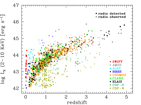
Figure 2: 2-10 keV de-absorbed luminosity, L_X, of the total sample as a function of redshift .

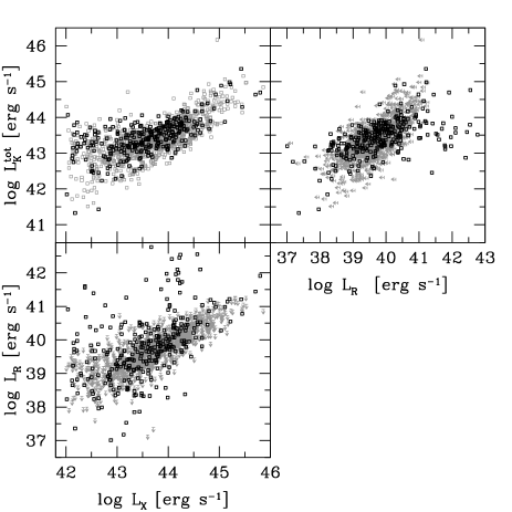
Figure 3: Distribution of the sample onto the 2D L_K-L_X, L${}_{K}^{tot}$-L_R and L_X-L_R planes, where L${}_{K}^{tot}$ is the total (galaxy + AGN) K-band luminosity. Squares represent the radio detected sources while the sources with a radio upper limit are shown by either grey arrows or grey squares (upper left panel).

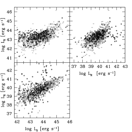
Figure 4: As in Figure 3 with L_K representing the AGN subtracted K-band galaxy luminosity.

4 The whole sample

In summary our data-set is composed by 9 X-ray selected AGN samples which contain a total of 1268 sources for which we were able to estimate the K-band stellar component luminosities of the host galaxy, L_K. For all these AGN, column densities and de-absorbed 2-10 keV luminosities, L_X, measures are available. The radio data allowed to measure on 293 sources the “nuclear” 1.4 GHz luminosity, L_R, while for the remaining sources 5$\sigma$ radio upper limits (Table 1, column 4) are available. In total, this is the largest catalogue of AGN (both of type 1 and 2) belonging to statistically well defined samples where radio, X and K band information exist. The distribution, in the L_X-$z$ plane of the whole AGN sample is shown in Figure 2, while in Figure 3 and Figure 4 we show the 3D L_K-L_X-L_R distribution, projected on to the three 2D L_K-L_X, L_K-L_R and L_X-L_R planes, where L_K is shown before (L${}_{K}^{tot}$), and after (L_K), the subtraction of the AGN component in the K-band, respectively.

5 The plane fitting

5.1 Maximum Likelihood fitting method

We have used a maximum likelihood fitting technique, with a Bayesian approach, in order to derive the probability distribution function of the AGN radio luminosity, L_R, as a function of L_X and the K band stellar component luminosity, L_K, $P(L_{R}|L_{X},L_{K})$. The maximum likelihood fitting method doesn’t need to use binning (as, e.g., it happens when using the $\chi^{2}$ fitting method), and therefore the results do not depend on the arrangement of the binning pattern. In the usual maximum likelihood fitting of luminosity function distributions $\rho(z,L)$ of extragalactic sources (eg. Marshall et al., 1983) the best fit solution is obtained by minimizing the quantity $S=-2ln\mathcal{L}$ (where $\mathcal{L}$ is the likelihood, and the $S$ function follows the $\chi^{2}$ statistic and therefore allows to estimates the confidence interval of the best fit parameters; Lampton, Margon & Bowyer, 1976). The natural logarithm of the likelihood function is computed as follows:

$$ln\mathcal{L}=\sum_{i}ln(\rho(z_{i},L_{i}))-\int\rho(z,L)\Omega(z,L){dV\over dz}dLdz,$$ (3)

where the sum is made over all the $i$ observed sources and $\Omega(z,L)$ is the sky coverage as function of the luminosity $L$ and redshift $z$. The first term is proportional to the combined probability (of independent events) of observing all the $i$ sources, each having redshift $z_{i}$ and luminosity $L_{i}$, while the second term corresponds to the total number of expected sources in the sample and is, therefore, also used to constrain the normalization of the luminosity function.

In our case we have devised a new $S$ function to be minimized which, following the same statistic principles of the maximum likelihood method, is able to measure the conditional probability distribution function $P(L_{R}|L_{X},L_{K})$ (where ${\int}P(L_{R}|L_{X},L_{K})dL_{R}=1$) of observing an $L_{R}$ radio luminosity in an object having $L_{X}$ and $L_{K}$ luminosities. Our method has the advantage (in comparison to other three-dimensional fitting techniques) to be also able to take into account the occurrence of upper limits in one of the three dimensions. Indeed, as already discussed, in all samples the radio observations are not deep enough do detect all the sources (see Table 1) and therefore upper limits need to be considered in order to derive the true AGN radio luminosity distribution (see Plotkin et al., 2012, for an analogous Bayesian approach on this topic). For these reasons the natural logarithm of the likelihood function has been computed as follows:

$$ln\mathcal{L}=\sum_{i}lnP(L_{R_{i}}|L_{X_{i}},L_{K_{i}})\ -$$

$$\sum_{j}\mathop{\int}_{L_{R}>L_{lim_{j}}}^{\infty}P(L_{R}|L_{X_{j}},L_{K_{j}})dL_{R}.$$

The first sum is computed for all the $i$ radio-detected sources and, as in eq. 3, is proportional to the combined probability of observing the radio luminosities L${}_{R_{i}}$ of all the $i$ detected sources, while the second term is the sum of the probability of radio detecting each $j$ observed (either radio detected or not) AGN, with a radio luminosity larger than its radio detection limit $L_{lim_{j}}$. In this case, analogously to the classical maximum likelihood method (eq. 3), this second term corresponds to the expected total number of radio detected sources.

5.2 The 3D Kolmogorov-Smirnov test

Although the maximum likelihood technique is very powerful in finding the parameters of the best fit solution and their uncertainties, it doesn’t allow to quantify how good the solution is. We have then devised a three-dimensional Kolmogorv-Smirnov (3D-KS) test able to measure the probability of observing the 3D distribution (in the $L_{R}-L_{X}-L_{K}$ space) of our sample of radio detected sources, under the null hypothesis that the data are drawn from the best fit model distribution.

The K-S test is a standard statistical test for deciding whether a set of data is consistent with a given probability distribution. In one dimension the K-S statistic is the maximum difference D between the cumulative distribution functions of the data and the model (or another sample). What makes the K-S statistic useful is that its distribution (in the case of the null hypothesis that the data are drawn from the same distribution) can be calculated giving the significance of any nonzero value of D.

Model	Function	$\xi_{X}$	$\xi_{K}$	$\xi_{0}$	Off-set	$\sigma_{l}^{1}$	$\sigma_{u}$	$a$	$k$	S	PKS
1	Gaussian	0.313	0.683	38.684	0.00	0.974	…	…	…	1583	2%
2	Double Gaussian	0.373	0.582	38.513	0.41	0.497	1.02	…	…	1571	3%
3	Lorentz	0.379	0.705	39.374	-0.43	1.141	0.30	…	…	1515	26%
4	Gaussian + exp	0.387	0.632	38.937	0.09	0.582	…	0.117	1.66	1504	35%
4	68% conf. errors	${}^{+0.031}_{-0.059}$	${}^{+0.066}_{-0.053}$	${}^{+0.050}_{-0.032}$		${}^{+0.028}_{-0.038}$		${}^{+0.087}_{-0.021}$	${}^{+0.24}_{-0.07}$
1) Corresponding to $\sigma$ in those models with a single spread parameter.

Table 2: Best fit solutions

In order to make a 3D-KS test we have followed the examples of the generalization of the K-S test to two-dimensional distributions by Peacock (1983) and Fasano & Franceschini (1987). The maximum difference D statistic has been computed by measuring the difference among the fraction of observed and expected (by the model) sources in each of the eight octants defined at the 3D positions of each radio detected source. In order to compute the number of expected sources, 2000 Monte Carlo simulations have been used. Although the 3D-KS test is carried out on the radio detected sample only, it properly takes into accounts the effects of the radio upper limits. Indeed, the simulations have been carried by extracting a radio luminosity (or not) for each observed source by taking into account its radio detection limits an the model conditional probability distribution function $P(L_{R}|L_{X},L_{K})$. The same 2000 simulations have been used to compute the probability (significance) to observe the measured maximum D statistic in the case of the null hypothesis that the data are drawn from the same distribution.

5.3 The fits

We have tried to fit the data assuming that the AGN radio luminosity, ${L_{R}}$, depends on average (i.e. with a spread in the radio luminosity axis) linearly from both the logarithmic X-ray and K-band (host galaxy) luminosities, drawing a plane in the 3D log$L_{R}$-log$L_{X}$-log$L_{K}$ space. As already discussed in the introduction, this assumption is suggested by the observations, done by many authors, of the existence of a BH fundamental plane: a similar relationship between the radio luminosity, the X-ray luminosity, and black hole mass ($M$), namely ${\rm log}L_{R}=\xi_{RX}{\rm log}L_{X}+\xi_{RM}{\rm log}M+constant$ (see Merloni, Heinz & di Matteo, 2003; Gültekin et al., 2009a). The AGN radio luminosity dependence on log$L_{X}$ and log$L_{K}$ was modeled by the following relationship:

$${\rm log}\bar{L_{R}}=\xi_{X}{\rm log}L_{X,44}+\xi_{K}{\rm log}L_{K,43}+\xi_{0},$$ (5)

where $\bar{L_{r}}$ is the luminosity of the peak (mode) of the probability distribution function of the spread in erg s^-1 units, and the luminosities have been normalized to $L_{X}=10^{44}{\rm erg~{}s}^{-1}L_{X,44}$ and $L_{K}=10^{43}{\rm erg~{}s}^{-1}L_{K,43}$.

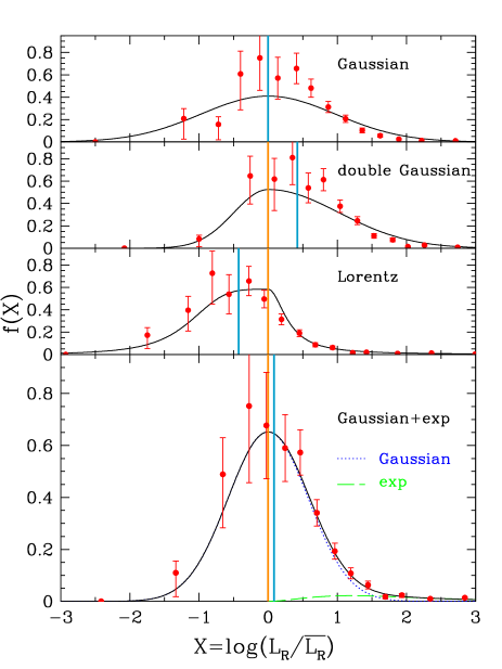
Figure 5: Probability distribution functions of $X={\rm log}(L_{R}/\bar{L_{R}})$, where $\bar{L_{r}}$ is the luminosity of the peak (mode), whose position is shown by a vertical continuous orange line. The four distributions correspond to the four best fits reported in Table 2. The blue vertical lines show the values of the means of the distributions, whose off-set from the peak luminosity is reported in Table 2, and which are used in the next figures to represent the best fit solutions.

This spread was first modeled by a Gaussian function, $G(X|0,\sigma)$, where $X={\rm log}(L_{R}/\bar{L_{R}})$, centered on $X=0$ with standard deviation $\sigma$. The best fit parameters are shown in Table 2 (model 1). However, the 3D-KS statistic tells that there is only a 2% probability that the observed distribution is drawn from the model. The probability distribution function of $X$ is shown in Fig. 5. The data have been plotted comparing in each bin of $X$ the number of observed ($N_{obs}$) and expected ($N_{exp}$; by the model) sources. This method ($N_{obs}$ vs. $N_{exp}$ method) reproduces the observations and consequently properly takes into account both the radio detections and the upper limits (see e.g. La Franca et al., 1994; La Franca & Cristiani, 1997; Matute et al., 2006, for similar applications). It is worth to note that this fit, although not satisfactory, gives and indication that the PDF of L_R is quite large: it results $\sigma\simeq 1$ dex. i.e. 68% of the cases are included into a 2 dex wide distribution. Similar results have been found by Merloni, Heinz & di Matteo (2003) and Gültekin et al. (2009a).

As shown in figure 5 (and already observed by La Franca, Melini & Fiore, 2010), the data show an excess of high radio luminosity sources if compared to a symmetrical distribution. In order to better take into account this excess we have assumed an a-symmetrical double Gaussian distribution with two $\sigma$ values: $\sigma_{l}$ and $\sigma_{u}$ for radio luminosities values below (lower) and above (upper) the value of the radio luminosity, $\bar{L_{r}}$, of the peak of the probability distribution (i.e. for $X$ values above or below zero) respectively. Indeed, the fit gives a larger spread, $\sigma_{u}$=1.0, at X$>$0, than measured at X$<$0, where $\sigma_{l}$= 0.5. However, even with this model, the 3D-KS test gives a not good enough, 3%, probability. As the PDF is a-symmetrical, we show in Figure 5 both the locus of the peak and of the mean of the PDF. A better representation of the model (e.g. in figures comparing the fit with the data) should, indeed, be carried out using the position of the mean of the distributions. The offsets between the mean and the mode (off-set = mean - mode) of the PDF are also listed in column 4 of Table 2.

Better results are obtained if the spread is modeled, as proposed by La Franca, Melini & Fiore (2010), assuming a double Lorentzian function described by the parameters $\sigma_{l}$ and $\sigma_{u}$:

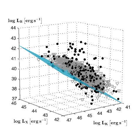
Figure 6: 3D distribution in the L_R-L_X-L_K space. Filled circles represent radio detections and faint open triangles represent radio upper limits. The plane of the distribution of the mean L_R as a function of L_X and L_K, according to the best fit solution 4 (Table 2), is shown.

$$P(X)=\left\{\begin{array}[]{l l}\frac{N}{A\pi\sigma_{l}\left[1+\left(\frac{X}{\sigma_{l}}\right)^{4}\right]}&\mbox{($X<0$)}\\ \\ \frac{A\ N}{\pi\sigma_{u}\left[1+\left(\frac{X}{\sigma_{u}}\right)^{2}\right]}&\mbox{($X\geq 0$),}\\ \end{array}\right.\$$ (9)

where, in order to obtain a continuous function at $X$$=$$0$, $A=\sqrt{\sigma_{u}/\sigma_{l}}$, and the parameter $N$ is constrained by the probability normalization requirement: $\int P(X)dX=1$. In this case (see Figure 5 and model 3 in Table 2) a 26% 3D-KS probability is obtained.

An even better solution is obtained if, for $X>0$, we add to a Gaussian distribution, $G(X|0,\sigma)$ (as in model 1), an exponential function able to reproduce the high radio luminosity tail,

$$P(X)=\left\{\begin{array}[]{rl}bG(X|0,\sigma)&\mbox{ ($X<0$)}\\ aX^{2}e^{-kX}+bG(X|0,\sigma)&\mbox{ ($X\geq 0$),}\\ \end{array}\right.$$ (10)

where the $a$ and $b$ parameters are not independent, as they are constrained by the probability normalization requirement

$$b=1-\int_{0}^{\infty}aX^{2}e^{-kX}dX.$$ (11)

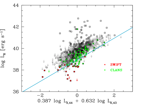
Figure 7: Edge-on view of the 3D plane. The more complete samples, SWIFT and CLANS, are represented by red and green squares, respectively. The continuous line shows the locus of the mean of the radio luminosity probability distribution function of our best fit solution 4 (Table 2). Radio upper limits are represented by arrows.

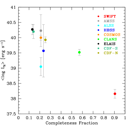
Figure 8: Mean radio luminosity of the radio detected sources of each sample as a function of the radio detection completeness.

The best fit solution (model 4 in Table 2 and see Figure 5) gives b=0.9499, which implies that the added exponential tail at high radio luminosities represents about 5% (1-0.9499) of the population (10% for X$\geq$0 where it is defined). In this case a 35% 3D-KS probability is obtained. As already shown by La Franca, Melini & Fiore (2010) the radio luminosity distribution of the AGN does not show any evidence of a bimodal distribution and therefore any definition of radio loudness is arbitrary. Nonetheless, it should be observed that (as demonstrated by these fits) the radio luminosity PDF is not symmetrical, but skewed with a long tail at high radio luminosities. The introduction of this tail at X$>$0 allows to obtain a narrower ($\sigma\sim 0.6$ dex) complementary symmetrical Gaussian distribution. The position of the peak of the radio distribution of our best fit solution (number 4) is represented by the following equation:

$${\rm log}\bar{L_{R}}=0.39^{+.03}_{-.06}{\rm log}L_{X,44}+0.63^{+.07}_{-.05}{\rm log}L_{K,43}+39.94^{+.05}_{-.03},$$ (12)

Confidence regions of each parameter were obtained by minimizing the $S$ function at a number of values around the best-fit solution, while leaving the other parameters free to float (see Lampton, Margon & Bowyer, 1976). The 68% confidence regions quoted correspond to $\Delta S$ (=$\Delta\chi^{2}$) = 1. The best fit solution is also shown in Figure 6, where the 3D distribution of the data is shown, and Figure 7, where the 2D edge on view of the plane is shown. This last figure helps understanding how much important is to take into account the effects of using censored data. The fitting solution seems, indeed, to be not a good representation of the distribution of the radio detections. This is because most of the X-ray samples have no radio observations able to detect all sources and then the radio detections are biased in favor of the most luminous radio sources. Indeed the mean radio luminosity of each of our samples decreases as a function of the radio identification completeness fraction: the average radio luminosity of the samples with about 10% radio identifications is of about logL_R=40.0 erg/s, while for the 90% complete samples the average luminosity is about 2 dex lower (logL_R=38.2 erg s^-1; see Figure 8). This bias is properly taken into account with our ML fitting method which takes into account upper limits. The fitting solution, indeed, fairly well reproduces the distribution of the most radio complete samples, such as SWIFT and CLANS (see Figures 7 and 9).

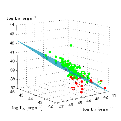
Figure 9: Same as Figure 6 but using only the, more radio complete, SWIFT (red circles) and CLANS (green circles) samples. Radio upper limits are represented by open triangles. The plane of the distribution of the mean L_R as a function of L_X and L_K, according to the best fit solution 4, is shown.

6 The AGN fundamental plane

Many authors have observed the existence of a BH fundamental plane relationship between the radio luminosity, the X-ray luminosity, and the BH mass (see the discussion in the Introduction). As a relation has been observed between the BH mass and the bulge luminosity, it is interesting to study whether the BH fundamental plane measures are compatible or not with our measured relationship in the log$L_{R}$-log$L_{X}$-log$L_{K}$ plane (we remember that L_K is the galaxy, stellar component, luminosity). We have therefore estimated the BH masses using the calibrated black hole versus K-band bulge luminosity relation from Graham (2007):

$$log(M_{bh}/M_{\odot})=-0.37(M_{K,bulge}+24)+8.29.$$ (13)

The bulge to total luminosity ratio (B/T), or the bulge to disc ratio (B/D; where $B/T=[1+D/B]^{-1}$) are function of the galaxy type (see Dong & De Robertis, 2006; Graham & Worley, 2008). Therefore, in order to properly derive the bulge luminosities from our measures of the total galaxy luminosities it would be necessary to know the morphological type of our galaxies. Unfortunately this information is barely available only for few tenths of galaxies belonging to the local sample (SWIFT), while for the higher redshift galaxies no information is available. Moreover, such a kind of relationships have been calibrated only on local samples, while it is well known that the average galaxy mass and morphology changes with redshifts (e.g. smaller and more clumpy galaxies with increasing redshift; Mosleh et al., 2012), and our sample reaches $z\sim 5$. However, our aim is not to measure the BH fundamental plane, but only to verify how much compatible our measure is with previous measures. According to Graham & Worley (2008), we have therefore assumed an average value of $B/T=1/4$ in the K bandpass (see e.g. Fiore et al., 2012, for similar assumptions). Under this assumption, eq. 13 corresponds to the relation

$${\rm log}(M_{bh}/M_{\odot})=0.925{\rm log}L_{K}-31.781,$$ (14)

where L_K is the total (bulge plus disk) galaxy luminosity, expressed in erg s^-1 units. We have compared our BH mass estimates with those reported by Merloni et al. (2010), which have been obtained via virial based analysis of optical spectra of AGN1. On average, our estimates are larger by 0.14 dex in solar masses with a spread of 0.43 dex, in solar mass units. This spread is compatible with the typical spreads ($\sim$0.3-0.4 dex) of the BH mass estimates based on both the virial and the scaling relations methods (Gültekin et al., 2009b), whose uncertainties, in our comparison, should be both taken into account in the propagation of errors.

According to eq. 14, our best fit solution 4 is transformed into the L_R-L_X-M_BH space in to the relation

$${\rm log}L_{R}=0.39{\rm log}L_{X}+0.68{\rm log}M_{BH}+16.61$$ (15)

while Merloni, Heinz & di Matteo (2003) measure

$${\rm log}L_{R}=0.60{\rm log}L_{X}+0.78{\rm log}M_{BH}+7.33,$$ (16)

where L_R here is the 5 GHz nuclear luminosity in units erg s^-1, with 1.4 GHz radio luminosities converted into 5 GHz $\nu$L_ν luminosities assuming a radio spectral index $\alpha=0.7$ (where L${}_{\nu}\propto\nu^{-\alpha}$; Condon, Cotton & Broderick, 2002), L_X the 2-10 keV nuclear X-ray luminosity in units of erg s^-1, and M_BH the black hole’s mass in units M_⊙ (Merloni, Heinz & di Matteo, 2003).

7 Discussion and Conclusions

As expected (see Figure 10), our estimate of the BH fundamental plane predicts lower radio luminosities if compared with the previous measure by Merloni, Heinz & di Matteo (2003). The typical difference, computed at 10⁸ M_⊙ BH mass and 10⁴⁴ erg s^-1 X-ray luminosity, is of $\sim$0.8 dex. As already observed in the L_R-L_X-L_K space, this difference is due to the inclusion in our analysis of the contribution of the radio upper limits, and indeed our best fit solution reproduces well the distribution of the most radio complete samples such as SWIFT and CLANS (Figures 11 and 12).

It should be noted that the fundamental plane of Merloni, Heinz & di Matteo (2003) was constructed by including a sample of X-ray BH binaries. While it is interesting to see that the mass scaling is still broadly consistent with that of Merloni, Heinz & di Matteo (2003) even in our study of an AGN-only sample, the radio-X-ray coefficient is very different: $\sim$0.4 in this study, while low-accretion rate (and low-luminosity) X-ray BH binaries show a tight radio-X-ray correlation with slope $\sim$0.6. Interestingly enough, recent re-analysis of radio-X-rays correlations in X-ray binaries suggests the presence of a second, less radio luminous branch (Gallo, Fender & Pooley, 2003; Coriat et al., 2011; Gallo, Miller & Fender, 2012). In this framework, our study, could suggest that, also in AGN, a second less radio luminous population should be taken into account, which could corresponds to those objects with low values of the $X={\rm log}(L_{R}/\bar{L_{R}})$ parameter (see Figure 5).

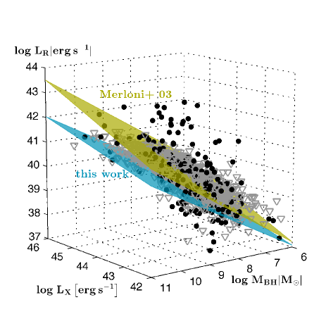
Figure 10: 3D distribution in the in L_R-L_X-M_BH space. The projection from the L_R-L_X-L_K space of the plane of the best fit solution 4 is shown in cyan. The fundamental plane from Merloni, Heinz & di Matteo (2003) is shown in gold. Radio upper limits are represented by open triangles.

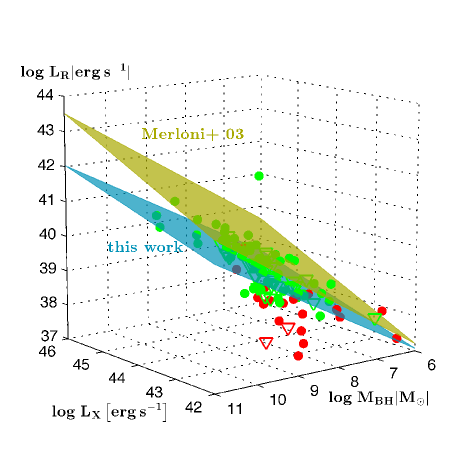
Figure 11: Same as Figure 10 but using only the, more radio complete, SWIFT (red circles) and CLANS (green circles) samples. Radio upper limits are represented by open triangles.

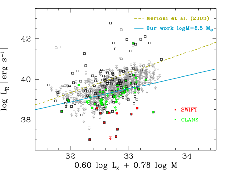
Figure 12: Edge on view of the BH fundamental plane as measured by Merloni, Heinz & di Matteo (2003) (gold dashed line). The continuous cyan line shows our solution for a sample of AGN having average logM=8.5. The more complete samples, SWIFT and CLANS, are represented by red and green squares, respectively. Radio upper limits are represented by arrows.

As already discussed in the Introduction, the measure of the dependence in AGN of L_R from other physical quantities such as L_X and the host galaxy K-band luminosity, L_K, is very useful in order to better include AGN in the galaxy evolution models where the AGN/galaxy feedback play a relevant role.

Our analysis has allowed to find a good analitical solution represented by a plane in the 3D logL_R-logL_X-logL_K space once a wide (1$\sigma$$\sim$1 dex), a-symmetrical, spread in the radio luminosity axis is included. This result confirms the study of La Franca, Melini & Fiore (2010), who, studying the dependence of PDF of L_R from L_X and $z$, where able to model the 1 dex wide (1$\sigma$) spread in the AGN radio luminosity distribution. This results show that a proper study of the correlation between different bands luminosities in AGN (or other sources) cannot be performed without taking into account censored data.

A clear example, in this framework, is the measure of the BH fundamental plane in the 3D logL_R-logL_X-logM space. After converting, using scaling relations, our measures of the host galaxy K-band luminosity into BH masses, our best fit solution corresponds to a BH fundamental plane which on average predicts 0.8 dex lower values for the AGN radio luminosities.

It should be pointed out that, at variance with many similar statistical studies, our analysis is based on a compilation of complete, hard X-ray selected, AGN samples, where both AGN1 and AGN2 are included. Therefore, our results should better represent the behaviour of the whole AGN population. However it will be interesting to check the 3D correlation between L_R, L_X and L_K in complete, radio selected samples. As the Merloni, Heinz & di Matteo (2003) sample was a hybrid sample without a clear selection criterion, it is plausible that parts of the differences found in the present work could be due to the specific selection criterion. In very general terms, if we do not believe we know any of the three terms (X-ray luminosity, radio luminosity and BH mass) as being the primary physical driver, all should be treated equal in a correlation study (but this is beyond the purposes of this paper).

In order to improve these analysis it would be very useful to obtain deeper radio observations of complete samples of AGNs combined with detailed optical-NIR-MIR SED observations. These data, when available, will eventually allow to measure the dependence of the radio luminosity distribution (i.e. the feedback) from the star and BH masses, their derivatives (star formation and accretion rates) and the redshift. A result that could be achieved by complementing multiwavelength surveys with observations carried out with new radio facilities such as the Expanded Very Large Array and the Square Kilometer Array.

8 Acknowledgments

We thank Andrea Merloni and Geoffrey Bicknell for discussions. We acknowledge the referee for his very careful review that allowed us to improve the quality of this work. This publication uses the NVSS and the FIRST radio surveys, carried out using the National Radio Astronomy Observatory Very Large Array. NRAO is operated by Associated University Inc., under cooperative agreement with the National Science Foundation. This publication makes use of data products from the Two Micron All Sky Survey, which is a joint project of the University of Massachusetts and the Infrared Processing and Analysis Center/California Institute of Technology, funded by the National Aeronautics and Space Administration and the National Science Foundation. We acknowledge financial contribution from PRIN-INAF 2011.

References

- Akiyama et al. (2003) Akiyama M., Ueda Y., Ohta K., Takahashi T., Yamada T., 2003, ApJ Supp, 148, 275
- Alexander et al. (2003) Alexander D. M. et al., 2003, AJ, 126, 539
- Baloković et al. (2012) Baloković M., Smolčić V., Ivezić Ž., Zamorani G., Schinnerer E., Kelly B. C., 2012, ApJ, 759, 30
- Becker, White & Helfand (1995) Becker R. H., White R. L., Helfand D. J., 1995, ApJ, 450, 559
- Bell et al. (2003) Bell E. F., McIntosh D. H., Katz N., Weinberg M. D., 2003, ApJ Supp, 149, 289
- Berta et al. (2006) Berta S. et al., 2006, A&A, 451, 881
- Best et al. (2006) Best P. N., Kaiser C. R., Heckman T. M., Kauffmann G., 2006, MNRAS, 368, L67
- Best et al. (2005) Best P. N., Kauffmann G., Heckman T. M., Brinchmann J., Charlot S., Ivezić Ž., White S. D. M., 2005, MNRAS, 362, 25
- Bianchi et al. (2009) Bianchi S., Bonilla N. F., Guainazzi M., Matt G., Ponti G., 2009, A&A, 501, 915
- Biggs & Ivison (2006) Biggs A. D., Ivison R. J., 2006, MNRAS, 371, 963
- Bongiorno et al. (2012) Bongiorno A. et al., 2012, ArXiv e-prints: 1209.1640
- Brinkmann et al. (2000) Brinkmann W., Laurent-Muehleisen S. A., Voges W., Siebert J., Becker R. H., Brotherton M. S., White R. L., Gregg M. D., 2000, A&A, 356, 445
- Brusa et al. (2010) Brusa M. et al., 2010, ApJ, 716, 348
- Brusadin (2003) Brusadin V., 2003, PhD Thesis, Univ. Roma Tre
- Cappelluti et al. (2009) Cappelluti N. et al., 2009, A&A, 497, 635
- Cattaneo & Best (2009) Cattaneo A., Best P. N., 2009, MNRAS, 395, 518
- Cattaneo et al. (2006) Cattaneo A., Dekel A., Devriendt J., Guiderdoni B., Blaizot J., 2006, MNRAS, 370, 1651
- Churazov et al. (2005) Churazov E., Sazonov S., Sunyaev R., Forman W., Jones C., Böhringer H., 2005, MNRAS, 363, L91
- Ciliegi et al. (2003) Ciliegi P., Zamorani G., Hasinger G., Lehmann I., Szokoly G., Wilson G., 2003, A&A, 398, 901
- Cocchia et al. (2007) Cocchia F. et al., 2007, A&A, 466, 31
- Condon, Cotton & Broderick (2002) Condon J. J., Cotton W. D., Broderick J. J., 2002, AJ, 124, 675
- Coriat et al. (2011) Coriat M. et al., 2011, MNRAS, 414, 677
- Croton et al. (2006) Croton D. J. et al., 2006, MNRAS, 365, 11
- Della Ceca et al. (2008) Della Ceca R. et al., 2008, A&A, 487, 119
- Dong & De Robertis (2006) Dong X. Y., De Robertis M. M., 2006, AJ, 131, 1236
- Dressler (1989) Dressler A., 1989, in IAU Symposium, Vol. 134, Active Galactic Nuclei, Osterbrock D. E., Miller J. S., eds., p. 217
- Falcke & Biermann (1995) Falcke H., Biermann P. L., 1995, A&A, 293, 665
- Falcke, Körding & Markoff (2004) Falcke H., Körding E., Markoff S., 2004, A&A, 414, 895
- Fanaroff & Riley (1974) Fanaroff B. L., Riley J. M., 1974, MNRAS, 167, 31P
- Fasano & Franceschini (1987) Fasano G., Franceschini A., 1987, MNRAS, 225, 155
- Feruglio et al. (2008) Feruglio C. et al., 2008, A&A, 488, 417
- Fiore et al. (2012) Fiore F. et al., 2012, A&A, 537, A16
- Gallo, Fender & Pooley (2003) Gallo E., Fender R. P., Pooley G. G., 2003, MNRAS, 344, 60
- Gallo, Miller & Fender (2012) Gallo E., Miller B. P., Fender R., 2012, MNRAS, 423, 590
- Graham (2007) Graham A. W., 2007, MNRAS, 379, 711
- Graham & Worley (2008) Graham A. W., Worley C. C., 2008, MNRAS, 388, 1708
- Granato & Danese (1994) Granato G. L., Danese L., 1994, MNRAS, 268, 235
- Grossan (1992) Grossan B. A., 1992, Ph.D. Thesis
- Gültekin et al. (2009a) Gültekin K., Cackett E. M., Miller J. M., Di Matteo T., Markoff S., Richstone D. O., 2009a, ApJ, 706, 404
- Gültekin et al. (2009b) Gültekin K. et al., 2009b, ApJ, 698, 198
- Heinz & Sunyaev (2003) Heinz S., Sunyaev R. A., 2003, MNRAS, 343, L59
- Kellermann et al. (1989) Kellermann K. I., Sramek R., Schmidt M., Shaffer D. B., Green R., 1989, AJ, 98, 1195
- Körding, Jester & Fender (2008) Körding E. G., Jester S., Fender R., 2008, MNRAS, 383, 277
- Kormendy & McClure (1993) Kormendy J., McClure R. D., 1993, AJ, 105, 1793
- Kormendy & Richstone (1995) Kormendy J., Richstone D., 1995, ARA&A, 33, 581
- La Franca & Cristiani (1997) La Franca F., Cristiani S., 1997, AJ, 113, 1517
- La Franca et al. (1994) La Franca F., Gregorini L., Cristiani S., de Ruiter H., Owen F., 1994, AJ, 108, 1548
- La Franca et al. (2004) La Franca F. et al., 2004, AJ, 127, 3075
- La Franca, Melini & Fiore (2010) La Franca F., Melini G., Fiore F., 2010, ApJ, 718, 368
- Lampton, Margon & Bowyer (1976) Lampton M., Margon B., Bowyer S., 1976, ApJ, 208, 177
- Laor & Behar (2008) Laor A., Behar E., 2008, MNRAS, 390, 847
- Madau, Pozzetti & Dickinson (1998) Madau P., Pozzetti L., Dickinson M., 1998, ApJ, 498, 106
- Magorrian et al. (1998) Magorrian J. et al., 1998, AJ, 115, 2285
- Maiolino & Rieke (1995) Maiolino R., Rieke G. H., 1995, ApJ, 454, 95
- Marconi et al. (2004) Marconi A., Risaliti G., Gilli R., Hunt L. K., Maiolino R., Salvati M., 2004, MNRAS, 351, 169
- Marshall et al. (1983) Marshall H. L., Tananbaum H., Avni Y., Zamorani G., 1983, ApJ, 269, 35
- Marulli et al. (2008) Marulli F., Bonoli S., Branchini E., Moscardini L., Springel V., 2008, MNRAS, 385, 1846
- Matute et al. (2006) Matute I., La Franca F., Pozzi F., Gruppioni C., Lari C., Zamorani G., 2006, A&A, 451, 443
- Merloni et al. (2010) Merloni A. et al., 2010, ApJ, 708, 137
- Merloni & Heinz (2008) Merloni A., Heinz S., 2008, MNRAS, 388, 1011
- Merloni, Heinz & di Matteo (2003) Merloni A., Heinz S., di Matteo T., 2003, MNRAS, 345, 1057
- Middelberg et al. (2008) Middelberg E. et al., 2008, AJ, 135, 1276
- Miller, Peacock & Mead (1990) Miller L., Peacock J. A., Mead A. R. G., 1990, MNRAS, 244, 207
- Miller et al. (2008) Miller N. A., Fomalont E. B., Kellermann K. I., Mainieri V., Norman C., Padovani P., Rosati P., Tozzi P., 2008, ApJ Supp, 179, 114
- Mosleh et al. (2012) Mosleh M. et al., 2012, ApJL, 756, L12
- Owen & Morrison (2008) Owen F. N., Morrison G. E., 2008, AJ, 136, 1889
- Panessa et al. (2007) Panessa F., Barcons X., Bassani L., Cappi M., Carrera F. J., Ho L. C., Pellegrini S., 2007, A&A, 467, 519
- Peacock (1983) Peacock J. A., 1983, MNRAS, 202, 615
- Plotkin et al. (2012) Plotkin R. M., Markoff S., Kelly B. C., Körding E., Anderson S. F., 2012, MNRAS, 419, 267
- Pozzi et al. (2007) Pozzi F. et al., 2007, A&A, 468, 603
- Pozzi et al. (2012) —, 2012, MNRAS, 423, 1909
- Puccetti et al. (2006) Puccetti S. et al., 2006, A&A, 457, 501
- Ranalli, Comastri & Setti (2003) Ranalli P., Comastri A., Setti G., 2003, A&A, 399, 39
- Sacchi et al. (2009) Sacchi N. et al., 2009, ApJ, 703, 1778
- Shankar et al. (2008) Shankar F., Cavaliere A., Cirasuolo M., Maraschi L., 2008, ApJ, 676, 131
- Silva, Maiolino & Granato (2004) Silva L., Maiolino R., Granato G. L., 2004, MNRAS, 355, 973
- Singal et al. (2011) Singal J., Petrosian V., Lawrence A., Stawarz Ł., 2011, ApJ, 743, 104
- Skrutskie et al. (2006) Skrutskie M. F. et al., 2006, AJ, 131, 1163
- Smolčić et al. (2009) Smolčić V. et al., 2009, ApJ, 696, 24
- Sutherland & Saunders (1992) Sutherland W., Saunders W., 1992, MNRAS, 259, 413
- Terashima & Wilson (2003) Terashima Y., Wilson A. S., 2003, ApJ, 583, 145
- Trouille et al. (2008) Trouille L., Barger A. J., Cowie L. L., Yang Y., Mushotzky R. F., 2008, ApJ Supp, 179, 1
- Tueller et al. (2008) Tueller J., Mushotzky R. F., Barthelmy S., Cannizzo J. K., Gehrels N., Markwardt C. B., Skinner G. K., Winter L. M., 2008, ApJ, 681, 113
- Ueda et al. (1999) Ueda Y. et al., 1999, ApJ, 518, 656
- Vasudevan & Fabian (2009) Vasudevan R. V., Fabian A. C., 2009, MNRAS, 392, 1124
- Vestergaard (2002) Vestergaard M., 2002, ApJ, 571, 733
- Watanabe et al. (2004) Watanabe C., Ohta K., Akiyama M., Ueda Y., 2004, ApJ, 610, 128
- Wuyts et al. (2008) Wuyts S., Labbé I., Schreiber N. M. F., Franx M., Rudnick G., Brammer G. B., van Dokkum P. G., 2008, ApJ, 682, 985