Theory of Quantum Phase Transition in Iron-based Superconductors with Half-Dirac Nodal Electron Fermi Surface

Abstract

The quantum phase transition in iron-based superconductors with ’half-Dirac’ node at the electron Fermi surface as a $T=0$ structural phase transition described in terms of nematic order is discussed. An effective low energy theory that describes half-Dirac nodal Fermions and their coupling to Ising nematic order that describes the phase transition is derived and analyzed using renormalization group (RG) study of the large-$N_{f}$ version of the theory. The inherent absence of Lorentz invariance of the theory leads to RG flow structure where the velocities $v_{F}$ and $v_{\Delta}$ at the paired half-Dirac nodes ($1\overline{1}$ and $2\overline{2}$) in general flow differently under RG, implying that the nodal electron gap is deformed and the $C_{4}$ symmetry is broken, explaining the structural (orthogonal to orthorhombic) phase transition at the quantum critical point (QCP). The theory is found to have Gaussian fixed point $\lambda^{*}=0,(v_{\Delta}/v_{F})^{*}=0$ with stable flow lines toward it, suggesting a second order nematic phase transition. Interpreting the fermion-Ising nematic boson interaction as a decay process of nematic Ising order parameter scalar field fluctuations into half-Dirac nodal fermions, I find that the theory surprisingly behaves as systems with dynamical critical exponent $z=1$, reflecting undamped quantum critical dynamics and emergent fully relativistic field theory arising from the non(fully)-relativistic field theory and is direct consequence of $(v_{\Delta}/v_{F})^{*}=0$ fixed point. The nematic critical fluctuations lead to remarkable change to the spectral function peak where at a critical point $\lambda_{c}$, directly related to nematic QCP, the central spectral peak collapses and splits into satellite spectral peaks around nodal point. The vanishing of the zero modes density of states leads to the undamped $z=1$ quantum critical dynamics.

I Introduction

Quantum phase transition in strongly correlated systems such as high $T_{c}$ superconductors is one of the most active topics in condensed matter physics. In cuprates and several families of the recently discovered iron-based family of high $T_{c}$ superconductors, there exists a quantum critical point at $T=0$ deep inside the superconducting dome that represents such quantum phase transition (Fig. 1a),b)). This QCP also separates tetragonal and orthorhombic crystal structures and thus represents structural phase transition at zero temperature. It has been argued that the orthorhombic state is described by the so-called Ising nematic order 1 7 8 and such structural transition in cuprates 2 3 and iron-based superconductors 4 5 6 (where $d$-wave symmetry was assumed) is nematic transition.

The general phase diagram of several families of iron-based superconductors 33 illustrated in Fig.1b) shows that there is a tetragonal to orthorhombic structural phase transition at some finite temperature in the undoped case down to $T=0$ at a critical doping $x_{c}$ deep inside the dome where the Ising nematic order coexists with the superconducting state. At $T=0$ this critical doping is a quantum critical point between Ising ordered state and Ising disordered state. The theory of quantum phase transition at this quantum critical point is the focus of this work.

The quantum phase transition in cuprates that relates structural phase transition with nematic order was first studied using renormalization group approach 11 12 which showed using perturbative RG calculation at fixed $N_{f}$ with $\epsilon$ expansion around $3+1$ dimensions that the velocity anisotropy in the nodal fermion action and the anisotropic coupling between nodal fermion and Ising nematic order leads to a fluctuation-induced first order phase transition, as indicated by the runaway RG flows.

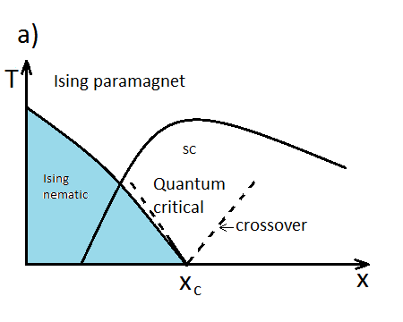
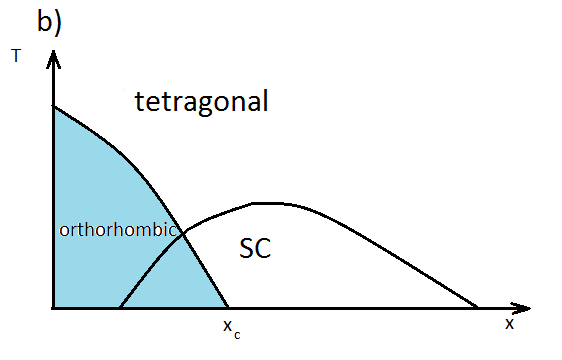
Figure 1: a) Quantum phase transition in cuprates with the quantum critical point and quantum critical region nearby. b) Typical phase diagram of iron-based superconductors with similar quantum critical point. In both a) and b), the parameter $x$ is defined as $x_{c}=-r$ and $x=-r(\lambda)$ as given in Eqs. (2) and (55). Physically, $x$ may represent doping level, pressure, or other appropriate experimental quantities.

A large-$N_{f}$ study of the same system but in $2+1$ dimensions 2 however found a second order quantum phase transition and has finite renormalized velocity anisotropy as compared to Dirac-like theory such as $QED_{3}$ which found velocity anisotropy to be irrelevant. Another RG study on the same system in $2+1$ dimensions 3 found vanishing velocity ratio $(v_{\Delta}/v_{F})^{*}=0$ as the fixed point.

The coupling between nodal quasiparticles to the nematic order was argued to be the most effective driving force of the structural transition. The presence of nodes and the resulting nodal quasiparticles in $d$-wave cuprates is therefore of crucial importance here. On the other hand, from the aspect of gap symmetry, iron-based family was originally thought to have isotropic $s_{\pm}$ wave symmetry, thus ruling out the presence of nodes. However it was found later that the electron Fermi pocket in iron-based superconductors admits anisotropic gap and thus permits existence of nodes.

In a related development, it has been shown recently that iron-based superconductors can have the so-called accidental (’zero’) node (Fig. 2) at the electron pocket 9 10 due to the gap anisotropy where the gap just touches the Fermi surface, that is, it is right at the onset of being gapless. In the simplest model, we can represent it by $\Delta(\theta)=\Delta_{0}(1-\cos 4\theta)$ (Fig. 2). Such accidental zero has anisotropic dispersion which in linear in $p_{x}$ direction and quadratic in $p_{y}$ direction or vice versa. One can therefore interpret such zero as ”half-Dirac” node, because it has Dirac spectrum in one direction but has parabolic dispersion in the perpendicular direction as that for free particle.

This accidental node is robust and persists to zero temperature where we can have a quantum phase transition between fully gapped (nodeless), zero and nodal states by tuning appropriate parameters, e.g. the coupling constants in the Hamiltonian 9 . Such gapless point is accidental because it does not arise from or protected by symmetry. This kind of nodes however has recently been shown to exist within finite regime of microscopic parameter space (the strength $\lambda_{h}$ of the inter-electron pockets hybridization) 23 and so this makes it interesting to study the nature of quantum phase transition in iron-based superconductor compounds with such peculiar gapless point. This is the purpose of this work.

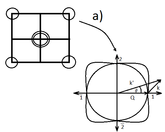
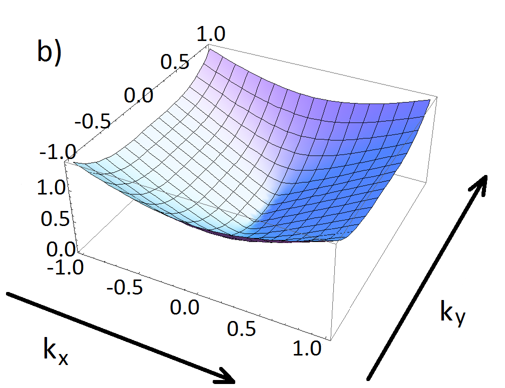
Figure 2: a) Iron-based superconductors’(reduced) Brillouin zone and the electron Fermi surfaces (’pockets’) at $(\pm\pi,\pm\pi)$ and hole pockets at $\Gamma=(0,0)$. The electron pocket has anisotropic gap and its critical half-Dirac nodes paired as $1\overline{1}$ and $2\overline{2}$. b) The profile of a half-Dirac node. Energy $E\sim k_{x}$ in $x$ direction but $E\sim k^{2}_{y}$ in $y$ direction.

I summarize my main results as follows. First, the quantum phase transition in iron-based superconductors with half-Dirac node described by half-Dirac fermion-Ising nematic field theory has stable fixed point $\lambda^{*}=0,(v_{\Delta}/v_{F})^{*}=0$ with no relevant interaction away from it in the $\lambda-v_{\Delta}/v_{F}$ parameter space and no nontrivial interacting fixed point. Second, on the dynamical properties of the quantum phase transition characterized in terms of response function describing quasiparticle-nematic coupling, I find that the system response effectively has dynamical critical exponent $z=1$. The nematic critical fluctuations lead to the splitting of the single quasiparticle spectral peak for small Yukawa coupling $\lambda<\lambda_{c}$ into two satellite spectral peaks for $\lambda>\lambda_{c}$, without affecting much the degree of spectral peak anisotropy. The central spectral peak collapses right at the nematic QCP, marking the vanishing of density of states at the nodal point, the gapping out of fermionic quasiparticles, and the emergence of fully relativistic effective field theory with the $z=1$ undamped quantum critical dynamics. The spectral peaks are however well defined away from QCP, both in ordered and disordered phases of nematic order. These latter results on spectral function are consistent with fixed point results as the $z=1$ field theory arises from the $(v_{\Delta}/v_{F})^{*}=0$ fixed point and the $\lambda_{c}$ reduces to $\lambda^{*}=0$ fixed point at the decoupled theory nematic QCP where the scalar field turns massless. This signifies novel quantum critical behavior of high $T_{c}$ superconductors with such half-Dirac nodes.

I begin the formulation of the theory that gives the above results in Section II by giving the low energy effective action for this problem, considering the large-$N_{f}$ version and computing the needed field theoretical quantities to proceed with the RG. Then I derive the RG fixed point structure and deduce the $\lambda-(v_{\Delta}/v_{F})$ RG phase diagram in Section III. I then discuss the nature of the quantum critical dynamics in terms of quasiparticle response and spectral functions in Section IV. I end with discussion of the results and connection with experiments.

II Low Energy Effective Field Theory

To describe half-Dirac nodes, we can start with standard Bogoliubov-de Gennes Hamiltonian describing nodal quasiparticles and approximate the Hamiltonian around the nodes in momentum space 9 . I then construct the effective low energy field theory action for the superconducting state - Ising nematic order phase transition which consists of the action for half-Dirac nodal fermionic quasiparticles part, scalar Ising (nematic) order part and the fermionic quasiparticle-Ising order interaction part. The fermions describe fermionic quasiparticles $\Psi,\overline{\Psi}$ living in the vicinity of half-Dirac nodes in electron Fermi surface while the Ising nematic scalar field $\phi$ describes the degree of lattice distortion from tetragonal lattice where $\langle\phi\rangle=0$ to orthorhombic lattice where $\langle\phi\rangle\neq 0$. The coupling between such nodal fermions with nematic order has been argued to be the most relevant coupling, i.e., the most effective process by which the nematic order field scatters the fermions around the nodes 11 .

In the actual physical situation, we have four fermion species for each of the pairs of (half-Dirac) nodes ($1\overline{1}$ and $2\overline{2}$), where we have spin up and down quasiparticles at one node and another set of spin up and down electrons at the partner node. In the $1/N_{f}$ technique, we generalize the spin up and down species into $N_{f}$ ”flavors” of fermions. The phenomenological field theory for this problem is then described by the following action

$$S_{\Psi}=\int\frac{d^{2}k}{(2\pi)^{2}}T\sum_{\omega_{m}}\sum_{a=1}^{N_{f}}\overline{\Psi}_{1,a}(-i\omega_{m}\gamma_{0}+v_{F}k_{x}\gamma_{1}+\frac{8v_{\Delta}}{k_{F}}k_{y}^{2}\gamma_{2})\Psi_{1,a}+\overline{\Psi}_{2,a}(-i\omega_{m}\gamma_{0}+v_{F}k_{y}\gamma_{1}+\frac{8v_{\Delta}}{k_{F}}k_{x}^{2}\gamma_{2})\Psi_{2,a}$$ (1)

$$S_{\phi}=\int d^{2}xd\tau(\frac{1}{2}(\nabla\phi)^{2}+\frac{1}{2}c^{2}(\partial_{\tau}\phi)^{2}+\frac{1}{2}r{\phi}^{2}+\frac{u}{4!}\phi^{4})$$ (2)

$$S_{\Psi\phi}=\lambda\int d^{2}x\int d\tau\phi\sum_{n=1,2,a=1}^{N_{f}}\overline{\Psi}_{n,a}\gamma_{0}\Psi_{n,a}$$ (3)

where

$$\Psi_{n,a}(\textbf{k}^{\prime},\omega_{n})=\left(c_{n,a,+}(\textbf{k}^{\prime},\omega_{m}),c^{{\dagger}}_{\overline{n},a,-}(-\textbf{k}^{\prime},-\omega_{m}),c_{\overline{n},a,+}(\textbf{k}^{\prime}-2\textbf{Q},\omega_{m}),c^{{\dagger}}_{n,a,-}(-\textbf{k}^{\prime}+2\textbf{Q},-\omega_{m})\right)^{T}$$ (4)

$$\overline{\Psi}_{n,a}=\Psi^{{\dagger}}_{n,a}\gamma_{0}$$

and

$$\gamma_{0}=\tau_{1}\bigotimes\sigma_{3},\gamma_{1}=i\tau_{2}\bigotimes\sigma_{0},\gamma_{2}=\tau_{1}\bigotimes i\sigma_{2}$$ (5)

where $\tau$ is Pauli matrix in ’node space’ ($1$ and $\overline{1}$ or $2$ and $\overline{2}$ as the basis states) while $\sigma$ is Pauli matrix in particle-hole (Nambu) space, with index $n=1,2$ representing the $1\overline{1},2\overline{2}$ pairs of nodes respectively, while $a=1,2,3,..,N_{f}$ is the fermion flavor index. In Eq. (4), $c_{n,a,+}$ for example represents annihilation operator for fermion from node $n$ with flavor $a,+$ where the $+$ represents analog of spin up while $c^{{\dagger}}_{\overline{n},a,-}$ represents creation operator for fermion from node $\overline{n}$ with flavor $a,-$ analog of spin down. The $\gamma$ matrices satisfy Dirac algebra $\{\gamma^{\mu},\gamma^{\nu}\}=2g^{\mu\nu}$ with metric $g^{\mu\nu}=\mathrm{diag}(1,-1,-1,-1)$. The momenta $\textbf{k}^{\prime},\textbf{Q}=k_{F}\hat{x}$ (for $1\overline{1}$ pair) or $\textbf{Q}=k_{F}\hat{y}$ (for $2\overline{2}$ pair), $\textbf{k}^{\prime}=\textbf{k}+\textbf{Q}$ are as defined in Fig. 2. The details to obtain the fermion action are given in Appendix A. It is necessary to emphasize that $N_{f}$ flavors do not imply spin $N_{f}$ quantum number. The $4\times 1$ Nambu spinor defined in Eq. (4) contains the two $N_{f}=2$ flavors from the two nodes in $1\overline{1}$ or $2\overline{2}$.

II.1 Symmetry Consideration and Character of Nematic Order

Nematic order is basically a $\textbf{Q}=0$ order that we have implicitly assumed to couple to spin singlet fermion bilinear. It can be characterized in terms of particle-hole and particle-particle pairing correlators,

$$\langle c^{{\dagger}}_{\textbf{k}^{\prime}\alpha}c_{\textbf{k}^{\prime}\alpha}\rangle=A_{\textbf{k}^{\prime}}$$

$$\langle c_{\textbf{k}^{\prime}\uparrow}c_{-\textbf{k}^{\prime}\downarrow}\rangle=(\Delta^{s}_{0}(-(\cos k^{\prime}_{x}+\cos k^{\prime}_{y})+(1+\cos k_{F}))+B_{\textbf{k}^{\prime}})e^{i\varphi}$$ (6)

where I have represented the half-Dirac nodal anisotropic $s$-wave gap as $\Delta(k^{\prime}_{x},k^{\prime}_{y})=\Delta^{s}_{0}(-(\cos k^{\prime}_{x}+\cos k^{\prime}_{y})+(1+\cos k_{F}))$. Here $\varphi$ is the overall superconducting phase and we assume superconducting background through the entire order-disordered phases of the nematic order parameter. An ideal electron Fermi surface of iron-based superconductors with square lattice, without any symmetry breaking interactions, has $C_{4}$ (or $C_{4v}$, which has extra symmetry of reflection with respect to vertical planes passing the central axis) symmetry.

It is to be noted that both charge neutral (ones that do not depend on the sign of the gap) and charged (ones that do) observables have this symmetry group, unlike in $d$-wave superconductors where only charge neutral observables have $C_{4v}$ whereas charged ones have only $C_{2v}$. This symmetry group has four $1d$ irreducible representations ($s$-wave with basis function $f(k^{\prime})=1$, $d_{x^{2}-y^{2}}$ ($\cos k^{\prime}_{x}-\cos k^{\prime}_{y}$), $d_{xy}$ $(\sin k^{\prime}_{x}\sin k^{\prime}_{y})$, and $g$ ($\sin k^{\prime}_{x}\sin k^{\prime}_{y}(\cos k^{\prime}_{x}-\cos k^{\prime}_{y})$) and one $2d$ irreducible representations $p(\sin k^{\prime}_{x},\sin k^{\prime}_{y})$ 11 . With $d$-wave pairing gap, it is clear that $A_{\textbf{k}^{\prime}}=0,B_{\textbf{k}^{\prime}}=\phi$ (where $\phi$ is real field) breaks $C_{4v}$ symmetry to $C_{2v}$. This is nematic order. So, symmetry arguments that characterize how nematic order couples to $d$-wave superconducting state suggest that nematic order parameter has $s$-wave symmetry where time-reversal symmetry is unbroken but the point group symmetry is reduced from $C_{4v}$ to $C_{2v}$ with basis function simply a unity function 11 . The nematic order can be polarized along $x$ or $y$ direction.

This extra $s$-wave component $\phi$ however will eliminate the half-Dirac nodes for $\phi>0$ or change each of the half-Dirac nodes to two full Dirac nodes for $\phi<0$. We can however have order parameter which breaks $C_{4v}$ to $C_{2v}$ while keeping the half-Dirac nodes intact which clearly must be higher order modes. From the 5 irreducible representations of $C_{4v}$ point group symmetry, $d_{xy}$ wave with basis function $\sin k^{\prime}_{x}\sin k^{\prime}_{y}$ in addition to an appropriate value of chosen constant can deliver such half-Dirac node-preserving $C_{4v}$-to-$C_{2v}$ symmetry breaking order parameter. To be precise, we can add on top of the anisotropic gap $\Delta(k^{\prime}_{x},k^{\prime}_{y})=\Delta^{s}_{0}(1+\cos k_{F}-(\cos k^{\prime}_{x}+\cos k^{\prime}_{y}))$ an order parameter $B_{\textbf{k}^{\prime}}=\phi_{0}+\phi\sin(k^{\prime}_{x})\sin(k^{\prime}_{y})$ where the gap will have half Dirac nodes shifted in its $k_{x},k_{y}$ by $0\leq k_{c}\leq k_{F}/\sqrt{2}$. The resulting gap for $\phi<0$ is shown in Fig. 3 while for $\phi>0$ the gap is Fig. 3 rotated by $\pi/2$. The structural tetragonal to orthorhombic phase transition can easily be seen by rotating the gap function by $\pi/4$ to align with the lattice $x$ and $y$ axes.

The order parameter fluctuations when coupled to fermions will be relevant only when the wavevector Q carried by the order parameter is also the wavevector Q that connects the two nodes between which the fermions are scattered, by momentum conservation 11 . That is, the order parameter will scatter the fermions effectively and efficiently only when the momentum it carries is transferred entirely to the fermions. Otherwise the scattering is a virtual process which merely renormalizes the coupling constant without making a fundamental change in low energy theory. In this case, nematic order corresponds to $\textbf{Q}=0$ which means my theory consider scattering of fermions living in the vicinity of the same half-Dirac node by the nematic order fluctuations.

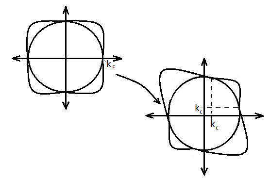
Figure 3: $C_{4v}$ to $C_{2v}$ symmetric breaking of electron Fermi pocket gap with half-Dirac nodes.

Scattering by $\textbf{Q}=(2k_{F},0)$ or $\textbf{Q}=(0,2k_{F})$ should be described by some type of density wave but if we want to couple this density wave with fermions, the theory should describe coexisting superconducting and density wave phases. I however would like to focus more on the interplay between nematic order and superconducting state described by Eqs. (1-3), which would be appropriate picture in several families of iron-based superconductor compounds 33 13 where density wave state does not coexist with superconducting state but nematic order does. I therefore essentially consider Ising-nematic quantum phase transition within the background superconductivity.

II.2 The Effective Action of Ising Nematic Order Parameter

In the large-$N_{f}$ expansion, with the physical case $N_{f}=2$ corresponds to spins up and down, we generalize the two spin polarizations of $S=1/2$ fermions into $N_{f}$ ”flavors” of fermions. I compute the effective action for bosonic nematic order parameter field $S_{eff}[\phi]$ by formally integrating out the fermion $\psi,\overline{\psi}$ from the original full action $S[\psi,\phi]$. This will give rise to nonlocal logarithmic term containing the fermion-nematic order field coupling constant $\lambda$ and can thus be expanded perturbatively in powers of $\lambda$, corresponding to the number of Yukawa vertices. The large $N_{f}$ expansion itself corresponds to expansion in number of loops.

$$S_{eff}[\phi]=S_{\phi}-N_{f}\sum_{n=1,2}\int_{\mathbf{k},\omega_{m}}\mathrm{log}(\mathrm{Det}[-i\omega_{m}\gamma_{0}+\mathbf{v}_{F}^{n}\cdot\mathbf{k}\gamma_{1}+\frac{8}{v_{\Delta}k_{F}}(\mathbf{v}_{\Delta}^{n}\cdot\textbf{k})^{2}\gamma_{2}+\lambda\phi\gamma_{0}])$$ (7)

Rescaling $\phi\rightarrow\frac{\phi}{\lambda}$ and $r\rightarrow rN_{f}\lambda^{2}$ Yukawacoupling and retaining the surviving terms, we have

$$S_{eff}[\phi]=N_{f}S^{1}_{eff}[\phi]$$

where

$$S^{1}_{eff}[\phi]=\int d^{3}x\frac{1}{2}r\phi^{2}-\sum_{n=1,2}\int_{\mathbf{k},\omega_{m}}\mathrm{log}(\mathrm{Det}[-i\omega_{m}\gamma_{0}+\mathbf{v}_{F}^{n}\cdot\textbf{k}\gamma_{1}+\frac{8}{v_{\Delta}k_{F}}(\mathbf{v}_{\Delta}^{n}\cdot\textbf{k})^{2}\gamma_{2}+\phi\gamma_{0}])$$ (8)

where the $(\partial_{\tau}\phi)^{2},(\nabla\phi)^{2},u\phi^{4}$ terms vanish as we take the $N_{f}\rightarrow\infty$ limit. I will only consider the quadratic correction terms in $\phi$ while assuming that the renormalized quartic terms will remain sufficient to stabilize the effective Ginzburg-Landau type effective theory for $\phi$ without explicitly considering its renormalization. The effective action to quadratic order for $\phi$ can be written as

$$S^{1}_{eff}[\phi]=\frac{1}{2}\int\frac{d^{3}k}{(2\pi)^{3}}(r+\Gamma_{2}(k))|\phi(k)|^{2}$$ (9)

where

$$\Gamma_{2}(k)=\Pi_{2}(k_{x},k_{y},\omega)+\Pi_{2}(k_{y},k_{x},\omega)$$ (10)

leading to scalar field propagator $D(k)=1/\left(r+\Gamma_{2}(k)\right)$. The polarization function $\Pi_{2}(k_{x},k_{y},\omega)$ is given by the Feynman diagram in Fig. 4.

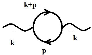
Figure 4: The Feynman diagram for polarization function which contributes correction to quadratic part of $\phi$ effective action.

Using the representation (5) for Dirac $\gamma$ matrices, the expression for the polarization function which is the correction to the boson propagator due to fermion is given by

$$\Pi_{2}(k_{x},k_{y},\omega)=\int\frac{d^{3}p}{(2\pi)^{3}}\mathrm{Tr}[\gamma_{0}G_{\Psi 0}(p)\gamma_{0}G_{\Psi 0}(p+k)]$$ (11)

with

$$G^{-1}_{\Psi 0}(p)=-i\omega\gamma_{0}+v_{F}p_{x}\gamma_{1}+\frac{8v_{\Delta}}{k_{F}}p_{y}^{2}\gamma_{2}$$ (12)

where we have focused only on node $1$ as example. Despite its lengthy form, this polarization function is still even under time reversal of external momenta $(k_{x},k_{y},\omega)\rightarrow(-k_{x},-k_{y},-\omega)$ which can be verified by direct inspection. Also, by power counting, this expression must have dimension one in external momenta $[\Pi_{2}(k)]=k^{1}$ but is an even function of $k=(k_{x},k_{y},\omega)$.

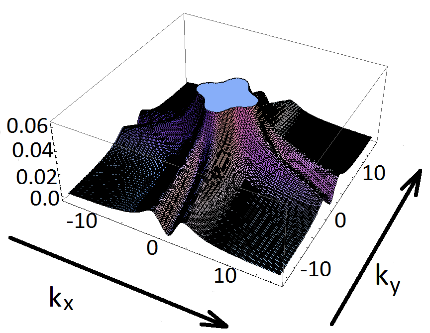
Figure 5: The profile of polarization function $\Gamma_{2}(k_{x},k_{y},\omega=-0.001\Delta\omega)$ computed numerically with $v_{F}=v_{\Delta}=0.067$eV$(a/\pi)$ where $a=0.1$ is the lattice spacing, with one unit of length $=100$ A^o. One unit of momentum $\Delta k=2\pi/10a$ and frequency $\Delta\omega=0.271$meV. Here we chop off the tip to show the symmetry of the profile. The function has even parity in $(\textbf{k},\omega)$ and $C_{4}$ symmetry.

I compute numerically the value of $\Gamma_{2}(k)$ in Eq. (10) as function of the two external momenta at a fixed external frequency and the result is shown in Fig. 5, which gives us some rough idea of how this quantity varies as function of momenta. The most important observation from Fig. 5 is that the polarization function profile has $C_{4}$ symmetry and that it is peaked around $\textbf{k}^{\prime}=(0,0)$ with respect to the center of electron pocket. I also compute the $1/N_{f}$ fermion self-energy and vertex corrections shown in Fig. 6 to nematic scalar field action needed for the following sections, the details of which are given in Appendix B. Self-energy renormalizes the fermion propagator,

$$G^{-1}_{\Psi}(p)=G^{-1}_{\Psi 0}(p)-\Sigma_{\Psi}(p)$$ (13)

with

$$\Sigma_{\Psi}(p)=\frac{\lambda^{2}}{N_{f}}\int\frac{d^{3}k}{(2\pi)^{3}}\gamma_{0}G_{\Psi}(p+k)\gamma_{0}D(k)$$ (14)

Regarding the nature of quantum phase transition, I will show that the quantum phase transition between Ising nematic ordered and disordered phases, in the presence of half-Dirac fermions in the background superconducting state, is second order phase transition with the non-interacting fixed point of Dirac fermions.

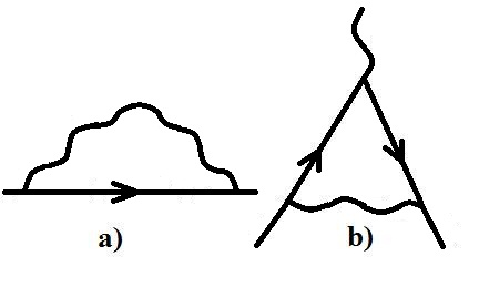
Figure 6: Feynman diagrams for a) fermion self-energy $\Sigma_{\Psi}(p)$ and b) Yukawa vertex $\Xi(p)$.

III Renormalization Group of the Theory

I will mainly be interested in the renormalization of the following two quantities: 1. The ratio of Fermi velocity $v_{F}$ and the ’gap velocity’ $v_{\Delta}$. 2. The fermion-boson Yukawa coupling $\lambda$. For the renormalization of velocities, the fixed point structure is deduced from the RG equations derived from logarithmic derivative of fermion self-energy 3 . For Yukawa coupling renormalization, two different methods are employed and shown to agree with each other. One is from RG equation derived from logarithmic derivative of Yukawa interaction vertex and the other is based on field theorist renormalization 17 . A $\lambda-(v_{\Delta}/v_{F})$ RG phase diagram is proposed at the end.

To begin, we consider scaling renormalization of fermion and boson fields and coupling constants at tree level. One thing that can be noticed from fermion action (1) is that the momentum is linear in $k_{x}$ but quadratic in $k_{y}$. If we want this action to be invariant under rescaling of momenta and frequency, the scaling dimension for $k_{x}$ must be twice of that of $k_{y}$. But here for the purpose of RG calculations we choose to use the same scaling dimension for $k_{x}$ and $k_{y}$. Further, rather than using a dynamical critical exponent $z$ for the scaling of frequency, we use the same scaling dimension for $\omega$ as that for $k_{x}$ and $k_{y}$. The reason is RG will naturally fix the scaling dimension for $\omega$ implicitly inside the coefficients of RG equations. Therefore, we write the scaling of momenta, frequency as follows;

$$k_{x}=k^{\prime}_{x}e^{-l}$$

$$k_{y}=k^{\prime}_{y}e^{-l}$$

$$\omega=\omega^{\prime}e^{-l}$$ (15)

The scaling of bosonic and fermionic scalar fields is obtained by considering renormalization of the time derivative term in $S_{\phi}$ and $S_{\psi}$ respectively which gives scaling dimensions $\mathrm{dim}[\Phi(k)]=-5/2$ and $\mathrm{dim}[\Psi(k)]=-2$. This suggests field scaling of the form

$$\Phi(k_{x},k_{y},\omega)=\Phi^{\prime}(k^{\prime}_{x},k^{\prime}_{y},\omega^{\prime})e^{\int_{0}^{l}dl^{\prime}(\frac{5}{2}-\frac{\eta_{b}}{2})}$$

$$\Psi(k_{x},k_{y},\omega)=\Psi^{\prime}(k^{\prime}_{x},k^{\prime}_{y},\omega^{\prime})e^{\int_{0}^{l}dl^{\prime}(2-\frac{\eta_{f}}{2})}$$ (16)

where $\eta_{b}$ and $\eta_{f}$ are boson scalar field and fermion field anomalous dimensions respectively. By similar simple power counting at tree level, where interaction is assumed to be nonsingular, as is the case here with Yukawa type of coupling, it can be easily checked that the scaling dimension of Yukawa coupling constant is $\mathrm{dim}[\lambda]=1/2$, leading to tree-level RG equation

$$\frac{d\lambda}{dl}=(\frac{1}{2}-\eta_{f}-\frac{\eta_{b}}{2})\lambda$$ (17)

with possibly nonzero fermion and boson anomalous dimensions included, which suggests that the coupling to nematic order parameter is most likely a relevant perturbation to a fixed point associated with the half-Dirac nodal fermions. The mass $r$ term on the other hand has scaling dimension $\mathrm{dim}[r]=1/\nu=2$ at tree level which shows it is also relevant parameter, the RG flow equation of which can in general be written as

$$\frac{dr}{dl}=\frac{1}{\nu}r=(2-\eta_{b})r$$ (18)

where the generally nonvanishing anomalous dimension $\eta_{b}$ of bosonic scalar field $\phi$ enters. Considering nematic criticality however, we eventually tune and fix it $r=0$ to investigate the RG flow of other parameters and coupling constants of interest in nematic critical regime.

As a comparison, one may prefer to use a rescaling of momenta and frequency that leaves the fermion action invariant,

$$k_{x}=k^{\prime}_{x}e^{-l}$$

$$k_{y}=k^{\prime}_{y}e^{-\frac{l}{2}}$$

$$\omega=\omega^{\prime}e^{-l}$$ (19)

Again considering renormalization of the time derivative term in $S_{\phi}$ and $S_{\psi}$ respectively gives scaling dimensions $\mathrm{dim}[\Phi(k)]=-9/4$ and $\mathrm{dim}[\Psi(k)]=-7/4$. This gives field scaling of the form

$$\Phi(k_{x},k_{y},\omega)=\Phi^{\prime}(k^{\prime}_{x},k^{\prime}_{y},\omega^{\prime})e^{\int_{0}^{l}dl^{\prime}(\frac{9}{4}-\frac{\eta_{b}}{2})}$$

$$\Psi(k_{x},k_{y},\omega)=\Psi^{\prime}(k^{\prime}_{x},k^{\prime}_{y},\omega^{\prime})e^{\int_{0}^{l}dl^{\prime}(\frac{7}{4}-\frac{\eta_{f}}{2})}$$ (20)

We will still arrive at the same conclusion that the Yukawa coupling is relevant perturbation away from a fixed point with tree-level scaling dimension of $\mathrm{dim}[\lambda]=3/4$. I will consider the renormalization of Fermi and gap velocities as well as the renormalization of Yukawa coupling in the following subsections.

III.1 Renormalization of Fermi and Gap Velocities

For velocity renormalization, I will prove that the field theory given by equations (1,2,3) has fixed point at $(v_{\Delta}/v_{F})^{*}=0$. I deduce this by considering RG equations derived from the logarithm of cutoff $\Lambda$ derivative of fermion self-energy and Yukawa vertex, which (for fermions from $1\overline{1}$ pair of nodes as example) take the form

$$\frac{d\Sigma}{d\mathrm{log}\Lambda}=(C_{0}^{0}\gamma_{0}+C_{1}^{0}\gamma_{1})(-i\omega)+(C_{0}^{1}\gamma_{0}+C_{1}^{1}\gamma_{1})v_{F}k_{x}$$

$$+(C^{0}_{2}\gamma_{0}+C^{1}_{2}\gamma_{1})\frac{8v_{\Delta}}{k_{F}}k^{2}_{y}$$ (21)

$$\frac{d\Xi}{d\mathrm{log}\Lambda}=C_{3}\gamma_{0}$$ (22)

Before proceeding further, we first find the relations between the $C$’s coefficients and the anomalous dimensions $\eta_{f}$ and $\eta_{b}$ Caveat .

The relation involving $\eta_{f}$ is obtained by fixing the kinetic time derivative part in $S_{\psi}$ while that for $\eta_{b}$ is obtained by fixing the Yukawa coupling term. The latter is done because the nematic order action $S_{\phi}$ does not have kinetic term upon integrating out the fermions, as can be seen in Eq. (8) which has a non-local term given by the logarithmic part. This non-local term will overpower the local terms of $S_{\phi}$ except the $r\phi^{2}$ term. This can be seen by considering the scaling dimensions of each of the terms in $S_{\phi}$. Earlier we obtained $\mathrm{dim}[\Phi(k)]=-5/2$ or $\mathrm{dim}[\phi(x,y,t)]=5/2$ and this gives $\mathrm{dim}[r]=2$ and $\mathrm{dim}[u]=1$. We see that the quartic coupling $u$ is less relevant than the quadratic coupling $r$ and so the former can be omitted. The derivative terms on the other hand will also have diminishing effect because they are marginal terms. We are therefore allowed to retain only the $r\phi^{2}$ and omit the other terms in $S_{\phi}$.

To find the relations between the $C$’s coefficients and the anomalous dimensions $\eta_{f}$ and $\eta_{b}$, we consider rescaling of appropriate terms in the actions Eqs. (1)(2)(3). I consider physical case with $N_{f}=2$ corresponding to spins up and down states where the $4\times 1$ spinor in Eq. (4) reads symbolically as $\Psi_{1}=\left(c_{1\uparrow},c^{{\dagger}}_{\overline{1}\downarrow},c_{\overline{1}\uparrow},c^{{\dagger}}_{1\downarrow}\right)^{T}$ for $1\overline{1}$ pair and similarly for $2\overline{2}$ pair. Fixing the kinetic time derivative part in $S_{\Psi}$, we have

$$\eta_{f}=-\gamma_{0}^{-1}\left(C_{0}^{0}\gamma_{0}+C_{1}^{0}\gamma_{1}\right)$$

$$=-\left(\begin{array}[]{cccc}C_{0}^{0}-C_{1}^{0}&0&0&0\\ 0&C_{0}^{0}+C_{1}^{0}&0&0\\ 0&0&C_{0}^{0}+C_{1}^{0}&0\\ 0&0&0&C_{0}^{0}-C_{1}^{0}\end{array}\right)$$ (23)

which demonstrates a ”pair-wise” pattern associating fermions living at the same nodes (fermions $1\uparrow$ and $1\downarrow$ at node 1 (or fermions $2\uparrow$ and $2\downarrow$ at node 2) and fermions $\overline{1}\downarrow$ and $\overline{1}\uparrow$ at node $\overline{1}$ (or fermions $\overline{2}\downarrow$ and $\overline{2}\uparrow$ at node $\overline{2}$). It is clear that the fermion anomalous dimension $\eta_{f}$ is a universal character which should be independent of the where the fermion lives in momentum space. With this, we then have

$$C_{0}^{0}-C_{1}^{0}=C_{0}^{0}+C_{1}^{0}=-\eta_{f}$$

and therefore

$$C_{0}^{0}=-\eta_{f},C_{1}^{0}=0$$ (24)

Following similar procedure to $\eta_{b}$ by fixing the Yukawa coupling, we have

$$C_{3}=-\left(\frac{1}{2}-\eta_{f}-\frac{1}{2}\eta_{b}\right)$$ (25)

One expects that $0\leq C^{\prime}s,\eta_{f}\ll 1$ as the $C^{\prime}s\sim\mathcal{O}\left(1/N_{f}\right)$ but as a result $\eta_{b}\sim 1$. We will discuss at the end of this subsection the RG flows of the $C^{0}_{0}$ and $C_{3}$ and consider first now the RG flows of the velocities, which are of immediate interest.

The RG equations for Fermi and gap velocities are derived by considering the renormalization of terms that contain these velocities in the fermion action $S_{\Psi}$. Fixing the $v_{F}k_{x}$ term, we have

$$\frac{dv_{F}}{dl}=\left(-\eta_{f}+\left(C_{0}^{1}\gamma_{1}^{-1}\gamma_{0}+C_{1}^{1}\right)\right)v_{F}$$ (26)

where $v_{F}=(v_{F1\uparrow},v_{F\overline{1}\downarrow},v_{F\overline{1}\uparrow},v_{F1\downarrow})^{T}$, whereas from renormalization of $\frac{8v_{\Delta}p_{y}^{2}}{k_{F}}$ term we have

$$\frac{dv_{\Delta}}{dl}=\left(-\eta_{f}+\left(C_{2}\gamma_{2}^{-1}\gamma_{0}+C_{2}\gamma_{2}^{-1}\gamma_{1}\right)\right)v_{\Delta}$$ (27)

where $l=-\mathrm{log}\Lambda$ RGsign , $v_{\Delta}=(v_{\Delta 1\uparrow},v_{\Delta\overline{1}\downarrow},v_{\Delta\overline{1}\uparrow},v_{\Delta 1\downarrow})^{T}$, in accordance to the $4\times 1$ spinor defined in Eq. (4) and without loss of generality, I have taken $C^{0}_{2}=C^{1}_{2}=C_{2}$. I only consider the leading linear order terms for the RG equations here. The RG flow parameter $l$ is defined in accordance with the Wilsonian RG philosophy where one incrementally integrates out momentum shell $e^{-l}\Lambda<k<\Lambda$ so that as $l$ goes to infinity, $\Lambda^{\prime}=e^{-l}\Lambda$ goes to zero. Using the $\gamma$ matrices as defined in (5), we obtain

$$\left(\begin{array}[]{cccc}\frac{dv_{F1\uparrow}}{dl}\\ \frac{dv_{F\overline{1}\downarrow}}{dl}\\ \frac{dv_{F\overline{1}\uparrow}}{dl}\\ \frac{dv_{F1\downarrow}}{dl}\end{array}\right)=\left(\begin{array}[]{cccc}M_{\alpha}&0&0&0\\ 0&M_{\beta}&0&0\\ 0&0&M_{\beta}&0\\ 0&0&0&M_{\alpha}\end{array}\right)\left(\begin{array}[]{cccc}v_{F1\uparrow}\\ v_{F\overline{1}\downarrow}\\ v_{F\overline{1}\uparrow}\\ v_{F1\downarrow}\end{array}\right)$$ (28)

where

$$M_{\alpha}=-\eta_{f}+C_{1}^{1}-C^{1}_{0},M_{\beta}=-\eta_{f}+C_{1}^{1}+C^{1}_{0}$$

$$\left(\begin{array}[]{cccc}\frac{dv_{\Delta 1\uparrow}}{dl}\\ \frac{dv_{\Delta\overline{1}\downarrow}}{dl}\\ \frac{dv_{\Delta\overline{1}\uparrow}}{dl}\\ \frac{dv_{\Delta 1\downarrow}}{dl}\end{array}\right)=\left(\begin{array}[]{cccc}-\eta_{f}&2C_{2}&0&0\\ 0&-\eta_{f}&0&0\\ 0&0&-\eta_{f}&0\\ 0&0&2C_{2}&-\eta_{f}\end{array}\right)\left(\begin{array}[]{cccc}v_{\Delta 1\uparrow}\\ v_{\Delta\overline{1}\downarrow}\\ v_{\Delta\overline{1}\uparrow}\\ v_{\Delta 1\downarrow}\end{array}\right)$$ (29)

We have RG flow equations for $v_{F}$ and $v_{\Delta}$ involving coefficients $C$’s that are themselves functions of $v_{F}$ and $v_{\Delta}$. We can see here that each of the four fermion components of the $4\times 1$ Nambu spinor has its own RG equations for $v_{F}$ and $v_{\Delta}$. This means that in general $v_{F}$ and $v_{\Delta}$ will flow differently between these four fermion components under RG. This feature arises purely from the symmetry property of anisotropic gap of electron pocket which is clearly different from $d$-wave cuprates case where one RG equation for $v_{F}$ and another RG equation for $v_{\Delta}$ are sufficient. If we consider the hypothesized fixed point $(v_{\Delta}/v_{F})^{*}=0$, which necessarily requires $(v_{\Delta})^{*}=0$ but $(v_{F})^{*}\neq 0$, from $dv_{F}/dl=0$ we will have $C_{0}^{1}=0$ and $C_{1}^{1}=\eta_{f}$ at the fixed point which set the final condition for the RG flow equation for the coefficients $C_{0}^{1}$ as $C_{0}^{1}(v_{\Delta}^{*}=0,v_{F}^{*}\neq 0)=0$ and $C_{1}^{1}$ as $C_{1}^{1}(v_{\Delta}^{*}=0,v_{F}^{*}\neq 0)=\eta_{f}$. This fixes the final condition for both coefficients in the RG flow for $v_{F}$. Considering the $dv_{\Delta}/dl=0$ at fixed point, we obtain no new information but the confirmation that the RG flow equation $dv_{\Delta}/dl$ is consistent at the fixed point. This consistency at least offers some posteriori justification of my fixed point assumption.

Now I present a more rigorous derivation of this fixed point result nonumerics . Eqs. (28) and (29) can be combined (relabeling $\left(n\uparrow,\overline{n}\downarrow,\overline{n}\uparrow,n\downarrow\right),n=1,2$ as $m=(1,2,3,4)$) to give

$$\frac{d\left(\frac{v_{\Delta m}}{v_{Fm}}\right)}{dl}=-\frac{1}{v_{Fm}}[-2C_{2}\left(\frac{v_{\Delta m}}{v_{Fm}}\right)s_{m}v_{\Delta_{m+t_{m}}}$$

$$+v_{\Delta m}\left(C^{1}_{1}(\frac{v_{\Delta m}}{v_{Fm}})+r_{m}C^{1}_{0}(\frac{v_{\Delta m}}{v_{Fm}})\right)]$$ (30)

where $s_{m}=1,r_{m}=-1$ for $n\uparrow,\downarrow$ (or $m=1$ and $4$) fermions and $s_{m}=0,r_{m}=1$ for $\overline{n}\uparrow,\downarrow$ (or $m=2$ and $3$) fermions while $t_{m}=+1,-1$ for $n\uparrow,\downarrow$ fermions respectively and $t_{m}=0$ for $\overline{n}\uparrow,\downarrow$ fermions. By comparing Eq. (21) and the explicit integral for self-energy Eq. (64) given in the Appendix, it can be seen that we must have $C^{1}_{0}=0$. This simplifies the final RG equations to as follows.

$$\frac{d\left(\frac{v_{\Delta 1}}{v_{F1}}\right)}{dl}=-\frac{1}{v_{F1}}[-2C_{2}\left(\frac{v_{\Delta 1}}{v_{F1}}\right)v_{\Delta 2}+v_{\Delta 1}C^{1}_{1}(\frac{v_{\Delta_{1}}}{v_{F1}}))]$$ (31)

$$\frac{d\left(\frac{v_{\Delta 2}}{v_{F2}}\right)}{dl}=-\frac{v_{\Delta 2}}{v_{F2}}C^{1}_{1}(\frac{v_{\Delta_{2}}}{v_{F2}})$$ (32)

$$\frac{d\left(\frac{v_{\Delta 3}}{v_{F3}}\right)}{dl}=-\frac{v_{\Delta 3}}{v_{F3}}C^{1}_{1}(\frac{v_{\Delta_{3}}}{v_{F3}})$$ (33)

$$\frac{d\left(\frac{v_{\Delta 4}}{v_{F4}}\right)}{dl}=-\frac{1}{v_{F4}}[-2C_{2}\left(\frac{v_{\Delta 4}}{v_{F4}}\right)v_{\Delta 3}+v_{\Delta 4}C^{1}_{1}(\frac{v_{\Delta_{4}}}{v_{F4}}))]$$ (34)

By directly comparing Eq. (21) and Eq. (64), we obtain

$$C^{1}_{1}=\frac{\lambda^{2}}{N_{f}}\frac{d}{d\mathrm{log}\Lambda}\int\frac{d^{3}p}{(2\pi)^{3}}\frac{1}{[(\omega+\Omega)^{2}+v_{F}^{2}(k_{x}+p_{x})^{2}+\xi^{2}(k_{y}+p_{y})^{4}]\Gamma_{2}(p)}$$ (35)

which is positive definite because the logarithmic cutoff derivative of the integral on the right hand side is positive since the integral is logarithmically divergent increasing function of cuttoff momenta $\Lambda$ (Note: $\xi=8v_{\Delta}/k_{F}$). This can be seen most easily by power counting of momenta in the numerator and denominator of the integral. In the UV limit $p=\Lambda\rightarrow\infty$, as to be shown in the next subsection, the $\Gamma_{2}(p)\sim 1/p$ and as the leading behavior in the denominator of the integral in Eq. (35) is dominated by the $p^{4}_{y}$ term, the net power of momenta-frequency of the integral is zero, corresponding to logarithmic divergence, with positive overall sign. Here, we consider the vicinity of QCP by setting $r=0$ and $\Gamma_{2}(p)$ is given by expression similar to Eq. (65). The RG equations (32) and (33) therefore flow to zero for arbitrarily small $v_{\Delta 2}/v_{F2}$ and $v_{\Delta 3}/v_{F3}$ respectively.

For Eqs. (31) and (34), there are two terms which compete with each other. The terms with $C_{2}$ couple the two equations with others so as to prevent simple inspection. However, again based on comparing Eq. (21) and Eq. (64), the $C_{2}$ is of relative order of magnitude $\mathcal{O}(v_{\Delta}/v_{F})$ whereas $C^{1}_{1}$ as we note above is of relative order of magnitude $\mathcal{O}(v_{F}/v_{F})\equiv\mathcal{O}(1)$. Therefore, the terms with $C^{1}_{1}$ in Eqs. (31) and (34) should dominate over terms with $C_{2}$, for arbitrarily small $v_{\Delta}/v_{F}$. This suggests that the right hand sides of Eqs. (31) and (34) are also negative definite and hence these RG equations also flow to zero for arbitrarily small $v_{\Delta 1}/v_{F1}$ and $v_{\Delta 4}/v_{F4}$ respectively. In conclusion, we have shown that the RG equations for the ratio of velocities $v_{\Delta}/v_{F}$ have fixed point at $(v_{\Delta}/v_{F})^{*}=0$.

Looking at the structure of the flow equations given in equations (28) and (29), we can see that the RG flow associated with the spin up nodal fermion at $(k_{F},0)$ is the same as that of spin down nodal fermion at $(k_{F},0)$. Likewise, the RG flow of the spin up nodal fermion at $(-k_{F},0)$ is identical to that of spin down nodal fermion at $(-k_{F},0)$. This agrees with the expectation that the Fermi velocity of two fermions living at the same half-Dirac node must flow identically but this also shows a new important observation that the Fermi velocity at the two half-Dirac nodes can in general flow differently under RG. One direct physical implication of Fermi velocity flowing to different values between fermions at different nodes is that, since $\epsilon_{k}=v_{F}k_{x}+O(k^{2})$ and $v_{\Delta}=\nabla_{k}\Delta(k)|_{\textbf{k}=(k_{F},0)}=\Delta_{0}/k_{F}$, the originally $C_{4}$ symmetric electron pocket gap is deformed under RG flows (where nematic order comes into play implicitly via its coupling to nodal Fermions) and thus the $C_{4}$ is broken (Fig. 3)).

For the completeness of results, now I discuss the RG flows of the coefficients $C^{0}_{0}$ which gives the flow of fermion anomalous dimension $\eta_{f}$ and $C_{3}$ which gives the Yukawa vertex RG equation in Eq. (22). I will show that both $C$’s have the correct definite sign that makes the $\eta_{f}$ and $\lambda$ themselves flow to zero at fixed point. This remarkable result can be deduced from the explicit expressions of the fermion self-energy and Yukawa vertex correction computed in the Appendix C in Eq. (64) and Appendix B Eq. (66) respectively, which when combined with Eqs. (21) and (22) give

$$C^{0}_{0}=-\eta_{f}=-\frac{\lambda^{2}}{N_{f}}\frac{d}{d\mathrm{log}\Lambda}\int\frac{d^{3}p}{(2\pi)^{3}}\frac{1}{[(\omega+\Omega)^{2}+v_{F}^{2}(k_{x}+p_{x})^{2}+\xi^{2}(k_{y}+p_{y})^{4}]}\frac{1}{\Gamma_{2}(p)}$$ (36)

$$\frac{d\lambda}{dl}=-\frac{d\lambda}{d\mathrm{log}\Lambda}=-C_{3}\lambda=-\frac{\lambda^{3}}{N_{f}}\frac{d}{d\mathrm{log}\Lambda}\int\frac{d^{3}p}{(2\pi)^{3}}\frac{\xi^{2}p^{4}_{y}-(\Omega^{2}_{m}-v^{2}_{F}p^{2}_{x})}{(\xi^{2}p^{4}_{y}+(\Omega^{2}_{m}+v^{2}_{F}p^{2}_{x}))^{2}}\frac{1}{\Gamma_{2}(p)}$$ (37)

with $\xi=8v_{\Delta}/k_{F}$, where I also have used Eqs. (17) and (25) to get Eq. (37). The integrals appearing in Eqs. (36) and (37) can be easily checked to be logarithmically divergent by power counting in the limit $p=\Lambda\rightarrow\infty$ where the $p_{y}$ terms dominate with $\Gamma_{2}(p)\sim 1/p$ and where again considering quantum criticality, $r=0$. The right hand side of the RG Eq. (36) for fermionic field $\Psi$ scaling is negative definite whereas that of Eq. (37) for $\lambda$ is zero to linear order in $\lambda$. This suggests marginal scaling behavior for $\lambda$ to linear order in $\lambda$ but the hypothesis that will be proven is that $\lambda$ is actually marginally irrelevant and that $\eta_{f}$ and $\lambda$ will flow to the fixed point $\eta^{*}_{f}=0,\lambda^{*}=0$ where $C^{0}_{0}$ and $C_{3}$ precisely vanish there. We see from Eqs. (35), (36), (37) that the $C$’s coefficients all vanish at the fixed point defined by $\lambda^{*}=0$. This, combined with Eqs. (24) and (25), thus predicts that $\eta^{*}_{f}=0,\eta^{*}_{b}=1$ at such fixed point.

To corroborate on this prediction, I present in the next subsection an equally powerful analysis using different method. To be precise, for this Yukawa coupling renormalization, I will show using field theorist renormalization scheme that the field theory given by equations $(\ref{eqn1},\ref{eqn2},\ref{eqn3})$ has a stable fixed point at $\lambda^{*}=0$ with the Yukawa coupling being a (marginally) irrelevant interaction, indicating that we have a second order phase transition. It will be demonstrated how these different calculations and analyses agree with each other so elegantly.

III.2 Renormalization of the Yukawa Coupling

In $d$-wave Cuprates, the relevance of nematic-quasiparticle Yukawa coupling at tree level led to the suggestion of the existence of a non-trivial fixed point $\lambda^{*}\neq 0$ along the coupling $\lambda$ axis 2 . I have shown earlier that with half-Dirac spectrum, Yukawa coupling to nematic order is apparently also relevant coupling at tree level with both choices of field rescaling. Therefore at tree level one would naively expect that $\lambda$ will flow away from the noninteracting Gaussian fixed point $\lambda^{*}=0$. However, we find that the theory for half-Dirac fermions has $\lambda^{*}=0$ fixed point at all orders in the number of loops, corresponding to orders in $1/N_{f}$. To show this, we use field theorist renormalization where we have to derive the $\beta$ function, which is nothing but (minus of) the right hand side of the usual Wilsonian RG equation, in the spirit of large-$N_{f}$ expansion, by considering all diagrams that give rise to divergence logarithmic .

Here we describe the details of renormalization of Yukawa coupling term $S_{\Psi\phi}$ using dimensional regularization with minimal subtraction scheme 17 . For a theory involving fermions and boson as we have in Eqs. (1, 2, 3), rewritten here for convenience in slightly different but equivalent form, the bare action is

$$S_{b}=\int_{k}\overline{\Psi}_{1,a}G^{-1}_{\Psi}(k_{x},k_{y},\omega)\Psi_{1,a}+(1\leftrightarrow 2,k_{x}\leftrightarrow k_{y})$$

$$+\int_{x}[\frac{1}{2}(\nabla\phi)^{2}+\frac{1}{2}c^{2}(\partial_{\tau}\phi)^{2}+\frac{1}{2}r_{0}{\phi}^{2}]+\frac{u_{0}}{4!}\phi^{4}$$

$$+\lambda_{0}\phi\overline{\Psi}_{n,a}\gamma_{0}\Psi_{n,a}$$ (38)

and we define the field rescaling as follows,

$$\Psi\rightarrow\sqrt{Z_{\psi}}\Psi,\phi\rightarrow\sqrt{Z_{\phi}}\phi$$

I rewrite the renormalized action as

$$S_{r}=\int_{k}Z_{\psi}\overline{\Psi}_{1,a}G^{-1}_{\Psi}(k_{x},k_{y},\omega)\Psi_{1,a}+(1\leftrightarrow 2,k_{x}\leftrightarrow k_{y})$$

$$+\int_{x}Z_{\phi}[\frac{1}{2}(\nabla\phi)^{2}+\frac{1}{2}c^{2}(\partial_{\tau}\phi)^{2}+\frac{1}{2}r_{0}{\phi}^{2}]+\frac{u_{0}}{4!}Z^{2}_{\phi}\phi^{4}$$

$$+\lambda_{0}Z_{\psi}Z^{1/2}_{\phi}\phi\overline{\Psi}_{n,a}\gamma_{0}\Psi_{n,a}$$

$$=S_{tree-level}+\delta S$$ (39)

where

$$S_{tree-level}=\int_{k}\overline{\Psi}_{1,a}G^{-1}_{\Psi}(k_{x},k_{y},\omega)\Psi_{1,a}+(1\leftrightarrow 2,k_{x}\leftrightarrow k_{y})$$

$$+\int_{x}[\frac{1}{2}(\nabla\phi)^{2}+\frac{1}{2}c^{2}(\partial_{\tau}\phi)^{2}+\frac{1}{2}r_{0}{\phi}^{2}]+\frac{u_{0}}{4!}\phi^{4}$$

$$+\lambda_{0}\phi\overline{\Psi}_{n,a}\gamma_{0}\Psi_{n,a}$$

$$\delta S=\int_{k}\delta Z_{\psi}\overline{\Psi}_{1,a}G^{-1}_{\Psi}(k_{x},k_{y},\omega)\Psi_{1,a}+(1\leftrightarrow 2,k_{x}\leftrightarrow k_{y})$$

$$+\int_{x}\delta Z_{r}[\frac{1}{2}(\nabla\phi)^{2}+\frac{1}{2}c^{2}(\partial_{\tau}\phi)^{2}+\frac{1}{2}r_{0}{\phi}^{2}]+\frac{u_{0}}{4!}\delta Z_{u}\phi^{4}$$

$$+\lambda_{0}\delta Z_{\lambda}\phi\overline{\Psi}_{n,a}\gamma_{0}\Psi_{n,a}$$ (40)

where we have defined $\delta Z_{\psi}=Z_{\psi}-1,\delta Z_{r}=Z_{\phi}-1,\delta Z_{u}=Z^{2}_{\phi}-1,\delta Z_{\lambda}=Z_{\psi}Z^{1/2}_{\phi}-1$. I have divided the renormalized action into ’tree-level’ action $S_{tree-level}$ and ’counter term’ action $\delta S$. The latter provides the renormalization corrections to the former. The need for renormalization arises because the interaction between fields operators and among themselves will modify (’renormalize’) the coupling constant of the interactions and the fields themselves. In most cases the interactions lead to divergent renormalization of those couplings and the fields. Since we start from field theory with finite coupling constants when they are noninteracting, the renormalized action is supposed to be also finite. To get such finite renormalized action, we just have to subtract off the infinities in the renormalized $S$ precisely with $\delta S$.

The change in coupling constant with the scale of renormalization is described by renomalization equation the most standard form of which is referred to as Callan-Symanzik equation 17 . It is well understood in QFT that only when the coupling constant correction $\sim\delta Z_{g}$ has UV divergence in the renormalization scale, the corresponding coupling constant $g$ where $g=r,u,\lambda$, will ’flow’ (in condensed matter physics terminology, or ’run’ in particle physics terminology) under renormalization to its low energy value. Under certain conditions, it will flow to some fixed point value. The renormalization scale to be used here is the momentum cutoff $\Lambda$ normally used regularize that UV divergence in the integral expression for Feynman diagrams that contribute to the renormalization. The renormalization equation takes the form

$$\frac{dg}{d\mathrm{log}\Lambda}=\beta(g)\sim\frac{d(Z_{g}-1)}{d\mathrm{log}\Lambda}$$ (41)

where the flow of the coupling is represented by ’beta function’ $\beta(g)$. The renormalization degree $\sim\delta Z_{g}=Z_{g}-1$ is given by the sum of all diagrams that contribute to the renormalization of coupling $g$. It is clear from the equation above that in order to get nonvanishing $\beta(g)$, the $\delta Z_{g}$ must be logarithmically divergent in $\Lambda$. Convergent $\delta Z_{g}\sim\Lambda^{-n},n>0$ will vanish as we take $\Lambda\rightarrow\infty$ and so will have no effect. Divergent $\delta Z_{g}$ by higher than logarithmic divergent will give infinite $\beta$ function which means the coupling constant either runs away to infinity when $\beta(g)\sim\alpha\Lambda^{n},\alpha>0,n>0,\beta(g)\rightarrow+\infty$ as $\Lambda\rightarrow\infty$, which is not physical, or quickly flows to zero when $\beta(g)\sim\alpha\Lambda^{n},\alpha<0,n>0,\beta(g)\rightarrow-\infty$ as $\Lambda\rightarrow\infty$, implying vanishing coupling (decoupled) fixed point.

To find the flow of a coupling constant, we therefore just have to evaluate all diagrams that contribute the renormalization of the corresponding coupling term in the action. For completeness, we will eventually consider all (lowest order) diagrams that contribute to the renormalization of all the coupling constants appearing in the action (39) as we go along, but we will finally be most interested in the renormalization of Yukawa coupling represented by $\lambda\phi\overline{\Psi}\gamma_{1}\Psi$ term. I will show that for half-Dirac fermion interacting with bosonic scalar field via Yukawa coupling, this Yukawa coupling renormalization has no logarithmic divergence at all orders in loop expansion (using diagrams all with bare rather than dressed propagators).

To begin the calculation, we start at one loop level where the Feynman diagrams in Fig. 4 ($\Gamma_{2}(k)$) contributes to renormalization factor $\delta Z_{r}$, Fig. 6 ($\Sigma_{\Psi}(p)$) contributes to renormalization factor $\delta Z_{\psi}$ and ($\Xi(k)$) contributes to renormalization factor $\delta Z_{\lambda}$, and Fig. 7 ($\Gamma_{4}(k)$) contributes to renormalization factor $\delta Z_{u}$.

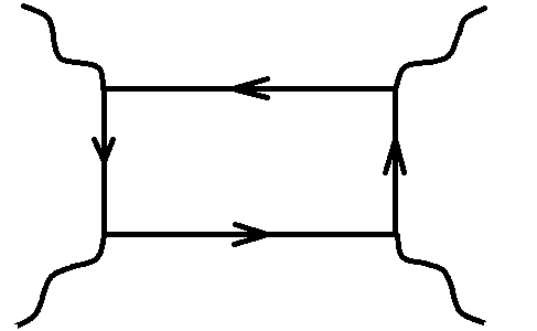
Figure 7: The Feynman diagram for 4-point correlation function $\Gamma_{4}(k)$ which contributes correction to quartic part of $\phi$ effective action.

To show the nondivergence of diagrams at all orders in $1/N_{f}$ (corresponding to number of loops), it suffices to consider the most potentially divergent diagrams. I start at one loop diagrams by considering the fermion self-energy $\Sigma_{\Psi}(p)$ as the most potentially divergent diagram because it only contains one fermion propagator in the loop. Since we are mainly looking for divergence, we need only look at the relative power of the momenta in numerator and denominator. The integral expression for $\Sigma_{\Psi}(p)$ in Eq. (14) is given in Eq. (64), rewritten here for convenience.

$$\Sigma_{\Psi}(k_{x},k_{y},\omega)=\frac{\lambda^{2}}{N_{f}}\int\frac{d^{3}p}{(2\pi)^{3}}\frac{i(\omega+\Omega)\gamma_{0}+v_{F}(k_{x}+p_{x})\gamma_{1}+\xi(k_{y}+p_{y})^{2}\gamma_{2}}{[(\omega+\Omega)^{2}+v_{F}^{2}(k_{x}+p_{x})^{2}+\xi^{2}(k_{y}+p_{y})^{4}]}\frac{1}{r}$$ (42)

where for consistency, we use bare propagator for both fermion and boson (that is, $\Gamma_{2}(k)$ is not included) so that the diagram is truly one loop diagram with unrenormalized internal propagators. The divergence or nondivergence of this diagram can be determined by computing the relative power of momenta and frequency in the numerator and denominator. It is to be noted that for quantum phase transition, which is a $T=0$ transition, we integrate the frequency $p_{0}\equiv\omega$ from $-\infty$ to $\infty$ and assuming continuum system, valid when correlation length is much larger than lattice spacing, which is valid in the vicinity of quantum phase transition, we also integrate the momenta $p_{1}\equiv p_{x},p_{2}\equiv p_{y}$ from $-\infty$ to $\infty$. In the presence of divergence, we will impose hard cutoff with UV cutoff $\Lambda$ which physically will be of the order of inverse microscopic lattice spacing of the system.

The integrand in $\Sigma_{\Psi}(p)$ is dominated by $p_{y}$ term in the limit $p_{x},p_{y},\Omega\rightarrow\Lambda\rightarrow\infty$ with net power for $p_{y}$ is $-2$. The result of integral will be of the form $\Sigma(p)\sim\int^{\Lambda}_{-\Lambda}d\omega\int^{\Lambda}_{-\Lambda}dk_{x}\int^{\Lambda}_{-\Lambda}dk_{y}/k^{2}_{y}\sim O(\Lambda)$ which suggests linearly divergent integral as $\Lambda\rightarrow\infty$. This however does not contribute to renormalization in minimal subtraction+dimensional regularization scheme, which relies on logarithmic divergence. We can actually interpret this as suggesting that the diagram has logarithmic divergence in $1+1$ dimensional theory. In other words, we are above the upper critical dimension, as the system is $2+1$ dimensional and that means the perturbation or fluctuations are irrelevant and we have stable fixed point.

Another diagram a must to consider in search of divergence is the polarization propagator $\Gamma(k)$(commonly referred to as 2-point function in QFT). Its expression is rewritten here for convenience.

$$\Gamma_{2}(k)=4\int\frac{d^{3}p}{(2\pi)^{3}}\frac{-\Omega(\Omega+\omega)+v_{F}^{2}p_{x}(p_{x}+k_{x})+\xi^{2}p_{y}^{2}(p_{y}+k_{y})^{2}}{((\Omega+\omega)^{2}+v_{F}^{2}(p_{x}+k_{x})^{2}+\xi^{2}(p_{y}+k_{y})^{4})(\Omega^{2}+v_{F}^{2}p_{x}^{2}+\xi^{2}p_{y}^{4})}+(x\leftrightarrow y)$$ (43)

I consider the integrand of Eq. (43) in the limit $p_{x},p_{y},\Omega=\Lambda\rightarrow\infty$. The numerator and denominator will be both dominated by the $p_{y}$ term where the net relative power of $p_{y}$ of the integrand is $-4$. The result of integral will be of the form $\Gamma_{2}(k)\sim\int^{\Lambda}_{-\Lambda}d\Omega\int^{\Lambda}_{-\Lambda}dp_{x}\int^{\Lambda}_{-\Lambda}dp_{y}/p^{4}_{y}\sim 1/\Lambda$ which suggests convergent integral as $\Lambda\rightarrow\infty$. Also, $\Gamma_{2}(k)\sim 1/k$ in the $k=\Lambda\rightarrow\infty$ limit. I used this result to argue for the negative definiteness of the function $C^{1}_{1}$ in Eq. (35). I also would like to stress that $\Gamma_{2}(k)$ has overall positive sign because it is dominated by the the $\xi^{2}p_{y}^{2}(p_{y}+k_{y})^{2}$ which of course has overall positive sign.

The remaining potentially divergent diagrams will be lower in power of momentum by 2 orders. Such diagram would be Yukawa vertex correction $\Xi(p)$ shown in Fig. 6 b) given by Eq. (66) because it has one more fermion propagator than self-energy diagram. In fact, since we are interested in the relevance or irrelevance of Yukawa coupling, this vertex correction is supposed to be the main diagram of interest. At one loop level with bare boson ($\Gamma_{2}(k)$ not included) and fermions propagators in the loop, the diagram will be convergent because the integral has net power of momentum of $-1$. All other diagrams at one loop and higher loop orders have more fermion propagators and are thus even more convergent. Since each fermion propagator asymptotically behaves as $\sim 1/p^{2}_{y}\sim 1/\Lambda^{2}$ in the limit $p_{x},p_{y},\Omega\rightarrow\Lambda\rightarrow\infty$, all other diagrams with more than one internal fermion propagators will have no divergence.

If however we reconsider Yukawa vertex correction $\Xi(p)$ and also self-energy $\Sigma_{\Psi}(p)$ expression Eq. (14) and use one-loop level dressed boson propagator $D(k)=1/(r+\Gamma_{2}(k))\sim 1/(r+\alpha/k)$ in the $k\rightarrow\infty$ limit, we see that these two quantities have logarithmic divergences in quantum critical regime where the scalar field is massless ($r=0$). In fact, I used precisely these logarithmic divergences to obtain the results in Eqs. (35), (36), and (37). These will be the only present logarithmic divergences if we replace all bare boson propagator with one-loop dressed boson propagator. It is therefore instructive to check what nontrivial renormalization would arise for a fermion-boson field theory with one logarithmic divergence in $2+1$ dimensional system. If we dimensionally regularize a logarithmically divergent integral in $2+1$ dimensions to general $d+1$-dimensions, we will have singularity in $\epsilon=2-d$ and the result for logarithmically divergent diagram is $C/\epsilon$ where $C\geq 0$ a positive constant. This gives rise to the following renormalization equations,

$$Z_{\phi}=1,Z_{\psi}Z^{1/2}_{\phi}\lambda_{0}=\lambda,Z_{\psi}G^{-1}_{\Psi}(p)-G^{-1}_{\Psi}(p)(1-C^{\prime}\frac{\lambda^{2}}{\epsilon})=0$$ (44)

for some constant $C^{\prime}=\alpha C,\alpha>0$ proportional to $C$, which gives

$$Z_{\psi}=1-C^{\prime}\frac{\lambda^{2}}{\epsilon},\lambda=\lambda_{0}(1-C^{\prime}\frac{\lambda^{2}}{\epsilon})$$ (45)

During RG flow, the UV cutoff $\Lambda$ will flow to smaller and smaller value, towards IR regime. I introduce a mass term $\mu$ to make the renormalized Yukawa coupling constant $\lambda$ dimensionless in $d$ dimensions by setting $\lambda_{0}=\mu^{\epsilon}f(\lambda)$ where $\lambda_{0},\lambda$ represent bare and renormalized Yukawa coupling constants, respectively. We can use the UV cutoff $\Lambda$ as mass parameter $\mu$ to conform with the discussion in Subsection III.A and the $\beta(\lambda)$ function is given by 17

$$\beta(\lambda)=-\frac{\epsilon f(\lambda)}{\frac{\partial f(\lambda)}{\partial\lambda}}=-\epsilon\lambda\frac{1-C^{\prime}\frac{\lambda^{2}}{\epsilon}}{1+C^{\prime}\frac{\lambda^{2}}{\epsilon}}$$ (46)

To lowest orders in $\epsilon$, this suggests RG equation of the form

$$\frac{d\lambda}{dl}=-\frac{d\lambda}{d\mathrm{log}\Lambda}=-\beta(\lambda)=\epsilon\lambda-2C^{\prime}\lambda^{3}+O(\lambda^{5})$$ (47)

where the RG flow parameter is defined as $l=-\mathrm{log}\Lambda$. This Eq. (47) matches precisely with Eq. (37) for $d=2$ $(\epsilon=0)$ and $2C^{\prime}=C_{3}$ and gives fixed point at $\lambda^{*}_{1}=0$ or $\lambda^{*}_{2}=\sqrt{\epsilon}/\sqrt{2C^{\prime}}$. The former is stable fixed point while the latter is unstable one for $\epsilon<0$ and conversely for $\epsilon>0$.

Figure 8: The RG $\beta$ function $-\beta(\lambda)$ vs. $\lambda$ of fermion-boson Yukawa coupling for a $(d=2-\epsilon>2)$-dimensional system with one logarithmic divergence.

Now we make a more physical consideration. High $T_{c}$ superconductors such as iron-based superconductors are of course 3-d but which are normally layered materials. This suggests that, they must be associated with an ’effective spatial dimension’ $2\leq d<3$, which means $\epsilon=2-d<0$. As we take $\epsilon\rightarrow 0$, $\lambda^{*}_{2}$ approaches $\lambda^{*}_{1}$. The stability of $\lambda^{*}_{1}=0$ fixed point and the unstability of $\lambda^{*}_{2}=\sqrt{\epsilon}/\sqrt{2C^{\prime}}$ for $\epsilon<0$ suggests that this $\lambda^{*}=0$ really prevails since intuitively, RG will flow away from $\lambda^{*}_{2}$ to $\lambda^{*}_{1}$. Besides, as we have seen in the Subsection IIIA. and will stress again here, $\lambda^{*}=0$ fixed point fits consistently with the RG flows of the C’s coefficients, anomalous dimensions, and the velocity ratio. Therefore, eventually we will have $\lambda^{*}=0$ as the prevailing and stable fixed point. Also, $\lambda^{*}=\infty$ possibility is automatically ruled out by this argument since such runaway flow will give similar runaway flows for the $C^{\prime}s$ and anomalous dimensions $\eta_{f},\eta_{b}$ (they will go to infinity) which will violate the equations relating them given in Subsection IIIA. To conclude, while Eq. (46) says at precisely $d=2$ ($\epsilon=0$), the $\beta$ function precisely vanishes and thus suggests marginal coupling, but instead of this unphysical strictly 2-d system conclusion, the physical realistic system consideration suggests that the Yukawa coupling should have tendency to flow towards noninteracting decoupled fixed point, rather than not flowing at all. To make this more discernible, a plot of $\beta(\lambda)$ vs. $\lambda$ is shown in Fig. 8, for $\epsilon=-0.1,C^{\prime}=1.0$ as example. Fig.  8 clearly shows the presence of stable fixed point at $\lambda^{*}=0$.

We note from the arguments in this subsection that this result on the irrelevance of Yukawa coupling and the stability of the Gaussian fixed point $\lambda^{*}=0$ holds at all orders in loop expansion, that is, at all orders in $1/N_{f}$. From the perspective of field theory renormalization, this is interesting result when compared to renormalization of Lorentz-invariant Dirac fermion theory of $QED_{3}$ with relativistic spectrum such as that in graphene 34 which normally has a critical number of fermion flavors $N_{c}$ which separates $N$’s which give first order phase transition and $N$’s which give second order phase transition. We can also compare it with other work describing nematic order in iron-based superconductors involving band fermions with quadratic dispersion in both $x$ and $y$ directions 35 , which similarly shows the presence of critical $N_{c}$. Half-Dirac fermions studied in this work thus behave differently compared to fully relativistic Dirac fermions or nonrelativistic fermions.

I will now show how we reconcile my field theorist renormalization result obtained earlier with the tree-level scaling result from Eq. (17) for half-Dirac fermion, which suggests tree-level RG equation for Yukawa coupling of the form

$$\frac{d\lambda}{dl}=(\frac{1}{2}-\eta_{f}-\frac{\eta_{b}}{2})\lambda$$ (48)

According to the large-$N_{f}$ effective action in Eqs. (7) and (8), we should evaluate the RG flow of boson mass parameter $r$ and Yukawa coupling $\lambda$. It is known 17 that for theory of fermion coupled to boson via Yukawa coupling, the RG equation for the Yukawa coupling constant $\lambda$ does not have dependance on the boson mass parameter $r$. We note that in Subsection III.A we obtained $\eta_{f}=C_{0}^{0},\eta_{b}=1+2C_{3}-2\eta_{f}$ where the $C$’s are coefficients appearing in RG equations of Fermi and gap velocities. The actual evaluation for these anomalous dimensions which requires explicit calculation of Feynman diagrams becomes prohibitive due to the non-Lorentz invariance of the field theory. However, we can readily see that for half-Dirac fermions, since the $C$’s coefficients must come from the large $N_{f}$ renormalization corrections to fermion and boson actions, but since both fermion self-energy $\Sigma_{\Psi}(p)$(which contributes to correction to fermion kinetic energy) and polarization bubble $\Gamma_{2}(k)$(which contributes to the correction to boson kinetic energy) have no logarithmic divergence, the $C$’s coefficients will vanish. This vanishing of $C$’s is precisely what we obtained from the RG analysis in Subsection III.A! Therefore the fermion and boson anomalous dimensions should precisely take value $\eta^{*}_{f}=0,\eta^{*}_{b}=1.0$ at the fixed point, which makes the right hand side of Eq. (48) equals to zero exactly. Any small positive $\eta_{f}$ and $\eta_{b}\geq 1$ will bring the system to flow towards decoupled fixed point. This suggests that a weak Yukawa coupling is (marginally) irrelevant, in complete agreement with the renormalization result obtained earlier.

This completes my proof that a weak Yukawa coupling between half-Dirac fermion and bosonic nematic order is not relevant perturbation with respect to the stable Gaussian fixed point at $\lambda^{*}=0$ and thus nematic quantum phase transition is second order phase transition. We arrive at the conclusion that with such accidental nodal non-Lorentzian fermion action, we have stable Gaussian fixed point, no matter what $N_{f}$ is, as the divergence is determined by the relative power of momenta in numerator and denominator, while power of $1/N_{f}$ enters as overall prefactor in front of integrals of n-point Feynman diagrams. Thus the field theory has $\lambda^{*}=0$ fixed point for all $N_{f}$ and at all orders in $1/N_{f}$ which means all orders in number of loops, including at one loop order. The result of this Section III can be summarized in an RG phase diagram in $\lambda-(v_{\Delta}/v_{F})$ plane Fig. 9. The diagram shows that we have fixed point at $\lambda^{*}=0,(v_{\Delta}/v_{F})^{*}=0$ and stable flow lines toward it.

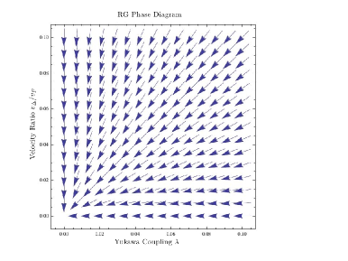
Figure 9: The RG phase diagram of the half-Dirac fermion-scalar field theory in the $\lambda-(v_{\Delta}/v_{F})$ plane for small enough $\lambda,(v_{\Delta}/v_{F})$. The $\lambda$ axis refers to appropriately normalized dimensionless Yukawa coupling $\lambda$.

One of the signatures of the proposed Ising nematic phase is its effect on the superconductor quasiparticle spectral function. In particular, quantum critical nematic fluctuations are expected to damp the quasiparticle spectral function, resulting in significant change in the spectra. In $d$-wave superconductor, it was shown 2 that quantum critical nematic fluctuations overdamps the quasiparticles in direction normal to the Fermi surface while weakly damps them in direction tangential to the Fermi surface around the node, resulting in highly anisotropic spectral function in the form of very narrow wedge. It is found in this work that in the case of iron-based superconductors with anisotropic gap in electron pocket, the situation is rather different.

IV The Nature of Quantum Critical Dynamics of the Theory

In this section, I investigate the nature of this quantum phase transition 16 15 from the system’s critical dynamics. The interaction between half-Dirac nodal quasiparticle and nematic Ising order field can be interpreted as damping process where Ising order parameter $\phi$ decays into half-Dirac nodal quasiparticles $\Psi$. One can then write a phenomenological field theory characterized by a dynamical critical exponent $z$ that measures the degree of the damping of the half-Dirac nodal quasiparticles by the nematic order parameter fluctuations. To quantify this dynamical process, I consider the finite temperature version of polarization function $\Gamma_{2}(\textbf{k},\omega_{m})$ in Eq. (10). Since polarization function can also be interpreted as susceptibility $\chi_{0}(\mathbf{k},\omega_{m})$ describing the system response, we can also use it to understand the nature of quantum critical phenomena from this dynamical property around the quantum critical point 24 25 at optimal doping level $x=x_{c}$, assuming that the half-Dirac node is kept intact by control of appropriate microscopic parameters. The susceptibility function $\chi_{0}(\mathbf{k},\omega_{m})$ applicable to the finite temperature crossover around QCP is given by

$$\chi_{0}(\mathbf{k},\omega_{m})=T\sum_{\Omega_{m}}\int\frac{d^{2}p}{(2\pi)^{2}}\mathrm{Tr}[\gamma_{0}G(p,\Omega_{m})\gamma_{0}G(p+k,\Omega_{m}+\omega_{m})]$$ (49)

where according to Eq. (10) we have to include the contribution of both pairs $1\overline{1}$ and $2\overline{2}$ of nodes. The quantum critical behavior is obtained by taking the $T\rightarrow 0$ limit of Eq. (49). The explicit expression for $\chi_{0}(k)$ is identical to that for $\Gamma_{2}(k)$ given in Eq. (65). The emphasis here is placed not on the explicit form of the above expression but rather, in its form upon lowest order expansion in powers of $k_{x},k_{y}$ and $\omega_{m}$ where $k_{x},k_{y}$ are measured from the node as shown in Fig. 2. By straightforward Taylor expansion of Eq. (65),

$$\chi_{0}(k_{x},k_{y},\omega_{m})\equiv\chi_{0}(k)$$

$$=\chi_{0}(0,0,0)+[k^{\mu}\frac{\partial\chi_{0}(k)}{\partial k_{\mu}}]_{k_{x}=k_{y}=\omega_{m}=0}$$

$$+\frac{1}{2}[k^{\mu}k^{\nu}\frac{\partial^{2}\chi_{0}(k)}{\partial k_{\mu}\partial k_{\nu}}]_{k_{x}=k_{y}=\omega_{m}=0}+...$$ (50)

we obtain

$$\chi_{0}(k_{x},k_{y},\omega_{m})=\chi_{0}(0,0,0)+a\omega_{m}^{2}+b(k_{x}^{2}+k_{y}^{2})+....$$ (51)

where the vanishing of linear in $k_{x},k_{y},\omega_{m}$ terms occurs because the resulting integrands obtained from taking $[k^{\mu}\partial\chi_{0}(k)/\partial k_{\mu}]_{k_{x}=k_{y}=\omega_{m}=0}$ in Eq. (65) are odd in $p_{x},p_{y},\Omega$. Eq. (51) shows the presence of kinetic term $\omega^{2}_{m}$ versus $k^{2}_{x},k^{2}_{y}$ and thus implies dynamical critical exponent $z=1$. We can contrast this with the Fermi liquid-spin density wave transition 15 for example which has low energy susceptibility of the form $\chi_{0}(\mathbf{k},\omega_{m})=\chi_{0}(0,0)-c_{1}|\omega_{m}|-c_{2}k^{2}+....$ where the $|\omega_{m}|$ indicates the damping of order parameter fluctuations due to the coupling to nodal fermions at the nodes connected by the spin density wave ordering wavevector. It is to be noted that I obtain the above result Eq. (51) even without taking the asymptotic limit $v_{\Delta}\rightarrow 0$ or making a priori assumption that we have fixed point at $(v_{\Delta}/v_{F})^{*}=0$. This therefore independently agrees with my earlier result that the field theory Eqs. (1,2,3) has fixed point at $(v_{\Delta}/v_{F})^{*}=0$ because then the fermions behave like those described by action $\sim\overline{\Psi}_{1,a}(-i\omega_{m}\gamma_{0}+v_{F}k_{x}\gamma_{1})\Psi_{1,a}+\overline{\Psi}_{2,a}(-i\omega_{m}\gamma_{0}+v_{F}k_{y}\gamma_{1})\Psi_{2,a}$ asymptotically in the limit $v_{\Delta}\rightarrow 0$ which has $z=1$. This is a crucial result of this work.

We observe here that despite having Lorentz-symmetry breaking anisotropic dispersion, in the low energy limit the Ising nematic field theory behaves as fully relativistic (i.e. with linear dispersion) undamped critical system characterized by $z=1$. This suggests the Ising nematic field fluctuations are effectively undamped by its coupling to half-Dirac nodal fermions. This is only possible if (or rather, this implies that), at nemating quantum critical point, the quasiparticle density of states is very low or actually vanishes. I will show quantitatively that this is indeed the case by directly computing the quasiparticle spectral function, which can be considered as generalized density of states. The spectral function is given by

$$A(\textbf{k},\omega)=-2\mathrm{sgn}(\omega)\mathrm{Im}[G_{\Psi,ab}(\textbf{k},\omega)]$$ (52)

where $G_{\Psi,ab}(\textbf{k},\omega)$ is the nonvanishing $(a,b)^{th}$ element of the renormalized single quasiparticle Green’s function given by $G^{-1}_{\Psi}(\textbf{k},\omega)=G^{-1}_{\Psi,0}(\textbf{k},\omega)-\Sigma_{\Psi}(\textbf{k},\omega)$. The $G_{\Psi,0}$ is given in Eq. (12) and the self-energy $\Sigma_{\Psi}(\textbf{k},\omega)$ can be decomposed as $\Sigma_{\Psi}(\textbf{k},\omega)=\Sigma^{a}\gamma_{0}+\Sigma^{b}\gamma_{1}+\Sigma^{c}\gamma_{2}$, the details of which are given in Appendix C. The resulting expression for quasiparticle spectral function is

$$A(\textbf{k},\omega)=2\mathrm{sgn}(\omega)\frac{\omega+\mathrm{Im}(\Sigma^{a}(\textbf{k},\omega))}{\left(\mathrm{Im}\left(\Sigma^{a}\left(\textbf{k},\omega\right)\right)+\omega\right)^{2}+\left(\Sigma^{b}\left(\textbf{k},\omega\right)-v_{F}k_{x}\right)^{2}+\left(\Sigma^{c}\left(\textbf{k},\omega\right)-\xi k_{y}^{2}\right)^{2}}$$ (53)

($\xi=8v_{\Delta}/k_{F}$) which for decoupled fermion-scalar field theory, obtained by setting the Yukawa coupling $\lambda$ to zero gives

$$A^{\lambda=0}(\textbf{k},\omega)=2\mathrm{sgn}(\omega)\frac{\omega}{\omega^{2}+v^{2}_{F}k^{2}_{x}+\xi^{2}k^{4}_{y}}$$ (54)

giving a spectral peak in $(k_{x},k_{y})$ plane at $(0,0)$ for fixed energy $\omega$. This fermion spectral function is modified by the coupling to nematic fluctuations as described by Eq. (53). The extent of the effect of nematic critical fluctuations on quasiparticles is best investigated by considering the dependence of spectral function on the strength of quasiparticle-nematic Yukawa coupling $\lambda$. The effect of nematic order on the fermions manifests itself in terms of the magnitude of spectral peak or the overall shape of $A(\mathbf{k},\omega)$ and one expects that there could be nontrivial change in the profile of spectral function near some critical value $\lambda=\lambda_{c}$ with regard to the presence or absence of Fermi arc. This can readily be expected from the fact that the effective action $S^{1}_{eff}[\phi]$ in Eq. (8), up to order $\mathrm{O}(\lambda^{2})$ in expansion of the logarithmic term, can eventually be written as

$$S^{1}_{eff}[\phi]=\frac{1}{2}\int\frac{d^{3}k}{(2\pi)^{3}}(r-r(\lambda))|\phi_{k}|^{2}+\ldots$$

$$\sim\frac{1}{2}\int\frac{d^{3}k}{(2\pi)^{3}}(\lambda_{c}^{2}-\lambda^{2})|\phi_{k}|^{2}+\ldots$$ (55)

where the mass parameter $r\sim\lambda^{2}_{c}$ corresponds to the critical coupling while $r(\lambda)\sim\lambda^{2}$ comes from the the Yukawa nematic-quasiparticle coupling. Intuitively speaking, for $\lambda\ll\lambda_{c}$ (deep inside disordered state of $\phi$), we have $\langle\phi\rangle=0$ and so that in computing the renormalized fermionic quasiparticle propagator we can simply substitute $\langle\phi\rangle=0$ for $\phi$. Likewise, for $\lambda\gg\lambda_{c}$ (deep inside ordered state), we have $\langle\phi\rangle\neq 0$ and we can simply substitute this $\langle\phi\rangle$ for $\phi$. In both cases, the quasiparticle spectral ridge is well defined.

The physics is more curious in the intermediate region near $\lambda_{c}$ as to what happens to the spectral peak and it expected that the decoupled theory central peak of spectral function may actually vanish. What this vanishing of spectral peak means will turn out that the single spectral peak in the decoupled $\lambda=0$ and weakly coupled $\lambda<\lambda_{c}$ cases splits into two (or perhaps more) spectral peaks. The spectral peak right at the half-Dirac node itself precisely vanishes and the spectral weight shifts to its surrounding points. One can get a hint on this behavior by analytically checking the expressions of Feynman diagrams contributing to renormalization. From Eqs. (53) and (67) in Appendix C, it is clear that $A(\textbf{k},\omega)$ vanishes at a critical value $\lambda_{c}$, which in the limit of $\lambda^{4}/r\ll 1$ and to order $\mathrm{O}(\lambda^{2})$, is approximately given by

$$\lambda^{2}_{c}=\frac{r|\omega|}{\int\frac{d^{3}p}{(2\pi)^{3}}\frac{(\omega+\Omega)}{[(\omega+\Omega)^{2}+v_{F}^{2}p^{2}_{x}+\xi^{2}p^{4}_{y}]}}$$ (56)

where I have focused on the nodal point ($k_{x}=k_{y}=0$) at which the peak is centered. At the next leading order in expansion in $\lambda$, we have $r(\lambda)$ containing $\lambda^{4}$ in Eq. (55) and $\lambda^{4}_{c}$ term on the left hand side of Eq. (56), as can be deduced from Eqs. (53) and (67), where $\Gamma_{2}(k)\sim\mathrm{O}(\lambda^{2})$ at one loop. Right at the nematic critical point of decoupled fermion-scalar field theory at which $r=0$, Eq. (56) gives us $\lambda_{c}=0$, which is nothing but the $\lambda^{*}=0$ fixed point we concluded in Section III. This is another point of consistency of the results.

Before going into numerics, to verify this intuitive picture on the physics in the $\lambda\approx\lambda_{c}$ and also in deep ordered and disordered phases, I consider the crude dependence of spectral function $A(\mathbf{k},\omega)$ on Yukawa coupling $\lambda$. From the expressions of self-energy components in Eqs. (67),(68),(69), we see that while their analytical closed forms are hard to obtain, for large $r$, they are all of $\mathcal{O}(\lambda^{2})$ as the leading $\lambda$ dependance (since they are obtained from one-loop Feynman diagram) plus subleading higher order $\lambda$ dependences, coming from the $\Gamma_{2}(p)$. So, to leading order in $\lambda$, we can write $\mathrm{Im}[\Sigma^{a}(\mathbf{k},\omega)]=\lambda^{2}f^{a}(\mathbf{k},\omega),\Sigma^{b}(\mathbf{k},\omega)=\lambda^{2}f^{b}(\mathbf{k},\omega),\Sigma^{c}(\mathbf{k},\omega)=\lambda^{2}f^{c}(\mathbf{k},\omega)$. With this, the spectral function becomes

$$A(\textbf{k},\omega)=2\mathrm{sgn}(\omega)\frac{\omega+\lambda^{2}f^{a}(\textbf{k},\omega))}{\left(\lambda^{2}f^{a}\left(\textbf{k},\omega\right)+\omega\right)^{2}+\left(\lambda^{2}f^{b}\left(\textbf{k},\omega\right)-v_{F}k_{x}\right)^{2}+\left(\lambda^{2}f^{c}\left(\textbf{k},\omega\right)-\xi k_{y}^{2}\right)^{2}}$$ (57)

We can already see from Eq. (57), small $\lambda$ ($\phi$-disordered state) will recover the sharp spectral function peak of decoupled half-Dirac fermion-scalar field theory of Eq. (54) shown in Fig. 10, while large $\lambda$ ($\phi$-ordered state) will broaden away this decoupled theory’s sharp spectral peak, change its magnitude, or produce more nontrivial change as mentioned above.

Figure 10: The quasiparticle spectral function $A(\textbf{k},\omega_{0})(\mathrm{meV})^{-1}$ centered at the node $1$ (Fig. 2) as function of $\lambda$ where the $\lambda$ increases from a) to d). To get these plots I have used $\omega_{0}=-1.54\mathrm{meV},T=0.01\mathrm{meV},a=10.0\mathrm{A}^{0},r=1000.0(\mathrm{meV})^{2},v_{F}=4v_{\Delta}=0.75\mathrm{eV}(a/\pi),\Lambda=\pi/a$ with $\lambda$ in unit of $\sqrt{\mathrm{meV}}$ k-plane . The central spectral peak for $\lambda<\lambda_{c}$ splits into satellite spectral peaks for $\lambda>\lambda_{c}$ at $\lambda_{c}\approx 700\sqrt{\mathrm{meV}}$.

Figure 11: The quasiparticle spectral function $A(\textbf{k},\omega_{0})(\mathrm{meV})^{-1}$ centered at the node $1$ (Fig. 2) as function of velocity anisotropy $v_{\Delta}/v_{F}$ where $v_{\Delta}/v_{F}$ increases from a) to d). To get these plots I have used $\omega_{0}=-1.54\mathrm{meV},T=0.01\mathrm{meV},a=10.0\mathrm{A}^{0},r=1000.0(\mathrm{meV})^{2},\lambda=1.0\sqrt{\mathrm{meV}},v_{F}=0.1875\mathrm{eV}(a/\pi),\Lambda=\pi/a$ k-plane .

To get explicit numerical result to support this analytical prediction, I compute numerically the spectral function as function of Yukawa nematic-fermion coupling strength $\lambda$. To appreciate the effect of such coupling, the spectral functions with and without such coupling are compared in Fig. 10. We observe that the spectral function has one sharp spectral peak in the $\phi$-disordered state ($\lambda<\lambda_{c}$) but which separates into subpeaks in the $\phi$ ordered state ($\lambda>\lambda_{c}$), corresponding to massive fermions. The central spectral peak collapses in the intermediate region, which directly corresponds to critical point $\lambda_{c}$ in $S^{1}_{eff}[\phi]$. It splits into two descendent satellite peaks that sit in the vicinity of the nodal point. This surprising behavior is one of the main results of this paper.

This $T=0$ critical point shows different behavior with regard to spectral peak than what occurs in thermal phase transition in cuprates where Fermi arc emerges as the temperature (here the Yukawa coupling $\lambda$ acts as temperature with $\lambda^{2}_{c}-\lambda^{2}\sim T-T_{KT}$) is increased above $T_{KT}$ in a Kosterlitz-Thouless type of transition when analyzed with $XY$ model 26 . In the QPT described by Eq. (55), in both deep ordered and disordered regions of $\phi$ field, the fermionic quasiparticles behave as free fermions (but being massive and massless respectively) and are well defined in these two. Right at the vicinity of the nematic quantum critical point, the quasiparticle density of states at the nodal point collapses and the quasiparticles are gapped, so that the zero energy quasiparticles vanish. This vanishing of zero energy density of states is also very reasonable to coincide with the transition into nematic ordered state since such order requires nonzero density of states of fermions with small but nonzero momentum transfer $\Delta\mathbf{k}$ for the fermions to be scattered, which is provided by the satellite spectral peaks.

This vanishing of zero modes is also precisely what is responsible for the ineffectiveness of Landau-damping mechanism, which results in an undamped quantum critical dynamics characterized by $z=1$ as predicted previously in Eq. (51). This gives rise to emergent fully relativistic field theory out of the originally non(fully)-relativistic field theory, as concluded earlier in this Section. This agreement is well-expected noting that the susceptibility function $\chi_{0}(k)\equiv\Gamma_{2}(k)$ given in Eq.(49) enters the definition of self-energy $\Sigma_{\Psi}(k)$ and thus the spectral function $A(k)$, where $k=(\mathbf{k},\omega_{m})$. This result underlines the difference of the physics of quantum and thermal phase transitions in these high $T_{c}$ superconductors and at the same time provides validity check to my theory.

Nematic critical fluctuations do not necessarily change much the degree of anisotropy of quasiparticle spectrum, but rather, the quasiparticle spectral weight itself, as we have just concluded. This is to be compared with the result for the $d$-wave case 2 which found a very strong damping of nematic order parameter by quasiparticle excitations in such a way that the spectral function of the quasiparticle is significantly broadened everywhere in Brillouin zone except at narrow ’wedges’ around Dirac nodes where the spectral function acquires a very anisotropic Fermi arc shape, being very narrow in direction perpendicular to the Fermi surface and very long in direction tangential to it. In other words, nematic critical fluctuations strongly enhance the velocity anisotropy of the $d$-wave nodal fermions. This later conclusion is however, as pointed out in 18 , very dependent on the use of nematic scalar field and tree level power counting result which casts the Yukawa coupling between nematic order and nodal quasiparticle as relevant.

I present here the dependence of quasiparticle spectral function on velocity ratio $v_{\Delta}/v_{F}$ shown in Fig. 11. It is to be noted that in the limit of $v_{F}\gg v_{\Delta}$, we have extremely anisotropic spectral weight along one of the two (e.g. $x$) orthogonal axes. As the ratio between the two velocities is tuned to order of unity, the anisotropy decreases but we still have relatively anisotropic spectral function. At $v_{F}\approx v_{\Delta}$ the spectral peak is actually still very anisotropic with ’Fermi arc’-like shape rather than round one. At the other limit of the anisotropy where $v_{\Delta}\gg v_{F}$, we have extremely anisotropic ridge perpendicular to the ridge in the opposite limit. This behavior clearly derives from the non-Lorentz symmetric form of fermion action. The spectral peak discussed in this Section will really take the shape of ’Fermi arc’ for the highly anisotropic case $(v_{\Delta}/v_{F})\rightarrow 0$, which was concluded in Section III to be the fixed point of the theory.

V Discussion and Summary

I have determined the RG fixed point structure of the low energy effective theory of half-Dirac iron-based superconductors to deduce its nematic quantum critical properties. By analyzing the RG equations for Fermi and gap velocities using symmetry arguments, I have shown that the field theory (1, 2, 3) has fixed point at $(v_{\Delta}/v_{F})^{*}=0$. This result is shown to be independently supported by analysis of the effect of critical nematic fluctuations on quasiparticle spectral function which reveals that the critical behavior has effective dynamical critical exponent $z=1$ which suggests precisely the same fixed point mentioned above. On the renormalization of Yukawa coupling, simple power counting at tree level apparently suggests that nematic order is relevant perturbation away from the decoupled fixed point of the half-Dirac fermion-nematic order field theory. However, all one-loop diagrams (with bare rather than dressed propagators) in the context of dimensional regularization plus minimal subtraction scheme of field theorist renormalization have no logarithmic divergence, and this extends to all orders in loop expansion. Eventually, the anomalous dimensions make the Yukawa coupling to be (marginally) irrelevant coupling that flows under renormalization towards noninteracting fixed point $\lambda^{*}=0$, suggesting second order structural quantum phase transition.

The Fermi and gap velocities at the four half-Dirac nodes around the electron Fermi pocket in general flow differently under RG. The $k_{x}\leftrightarrow k_{y}$ equivalence of $C_{4}$ symmetry is broken by this anisotropy and this suggests that the gap deformation instability associated with nematic order is the phenomenological physical picture of structural phase transition in half Dirac nodal iron-based superconductors. The whole analysis assumed that the half-Dirac nodes remain intact all along during RG flow. The possibility for this to be the real situation is strongly supported by recent work in Ref. 23 where it was shown the such kind of nodes is guaranteed to exist as long as the strength $\lambda^{h}$ of hybridization between the two electron pockets (the interpocket hopping term with momentum $(\pi,\pi,\pi)$) is less than some critical value $\lambda^{h}_{c}$. My theory is therefore valid within finite regime in parameter space rather than only at a critical point that can only be achieved by fine tuning.

In describing the physical mechanism of structural phase transition in high $T_{c}$ superconductors, the nematic phase couples most relevantly to the quasiparticles while at the same time couples to lattice distortion which measures the degree of structural deformation. The nematic phase can be electronic (charge) or spin nematic phase, which is an intensively studied theoretical question FernandesNatPhys and is also currently actively investigated experimentally 21 . The gap anisotropy in iron-based superconductors is believed to be determined by orbital content 22 of the electron Fermi pocket and this directly suggests connection of structural phase transition to orbital ordering as orbital ordering is driven by redistribution of occupation density of $d_{xz}$ and $d_{yz}$ orbitals in $(\pi,0)$ and $(0,\pi)$ electron pockets (in extended Brillouin zone). We see therefore a self-consistency of picture of the physics of structural phase transition as related to the symmetry breaking of anisotropic gap on the electron pocket with the proposal of orbital ordering-driven structural phase transition. It was also shown that in orbital ordering picture 14 the structural phase transition is in the Ising universality class and can be described by effective Hamiltonian

$$H_{SPT}=-J_{SPT}\sum_{\langle i,j\rangle}M_{i}M_{j}$$ (58)

which is consistent with my Ising nematic ordering picture and idea that nematic ordering can be related to orbital ordering.

Universality of properties of iron-based superconductors has been an important issue. Some properties are specific to certain families of iron-based compounds and not applicable to others. This consequently has important implications to the applicability of theoretical works on iron-based superconductivity. My theory here is therefore not expected to be applicable to all types of iron-based superconductors, but only to certain families of compounds satisfying particular requirements. I therefore would like to give precise details on what conditions and to which families of iron-based superconductors my theory are useful the most.

My theory is directly relevant to families of compounds where there is a structural tetragonal to orthorhombic phase transition that goes well into the superconducting dome, irrespective of the presence or absence of closely-following magnetic ordering transition. This condition turns out to occur precisely in the 122 family such as $Be(Fe_{1-x}Co_{x})_{2}As_{2}$, as reported in Refs. 27 and 28 where the phase diagram shows the same global features as we assumed in this work. This also occurs in 1111 family as published in Ref. 29 which reported the structural phase transition in 1111 iron-pnictide family where upon doping, the magnetic ordered phase vanishes before superconductivity emerges and there is thus no coexistence and we can forget about antiferromagnetic state once we are inside superconducting state. However, the structural phase transition penetrates into superconducting dome precisely as we assumed, and the paper argued that the perfection of tetrahedron in the atomic configuration is important for superconductivity. This provides hint that structural distortion is against superconductivity and this suggests coupling between superconductivity and structural distortion. This clearly supports my idea of coupling superconductivity and nematic order. This pattern of phase transition also occurs in 11 family as reported in Ref. 30 which demonstrated that structural phase transition occurs in 11 iron-chalcogenide $Fe_{1.01}Se$ compound within superconducting state. Also the paper argued that magnetism is not the driver of structural phase transition and this suggests the presence of intrinsic nematic order that interacts with superconducting state in producing the observed structural deformation.

Another condition for the relevance of my theory is that the electron gap must necessarily be anisotropic. As mentioned, while it was originally thought that iron-based superconductors were isotropic $s_{\pm}$, it became evident from later experiments that the electron gap is actually anisotropic; function of angle around the circular Fermi surface. This turns out to be the case in 122 family of compounds such as that in Ref. 31 which reported anisotropy in in-plane resistivity of $BaFe_{2}As_{2}$ and argued that this cannot derive from the too weak effect of spin order or lattice distortion but rather, this must come from gap anisotropy, precisely the hypothesis of my work. Even better is if we have 4-fold gap anisotropy. This is precisely the case in iron-chalcogenide compound $FeTe_{0.6}Se_{0.6}$ studied in Ref. 32 which reported anisotropic gap symmetry with precisely the same form as assumed in this paper although in their case the gap is nodeless.

The main results of this work can be directly experimentally tested. The main challenge is of course to find iron-based superconducting compounds that have the electron gap with the structure assumed in this work. The next step is to make sure that the compounds display structural phase transition that occurs all the way inside the superconducting dome up to a critical doping at $T=0$. Once these situations are established, the quantum critical and quasiparticle properties predicted in this work can be directly verified.

Appendix A Details on the Fermion Action

Figure 12: Electron Fermi surface with critical half-Dirac node

I will give the details here the construction of fermionic quasiparticles action. I consider electron pocket with anisotropic gap associated with the fermionic quasiparticles, as illustrated in Fig. 12. The ’nesting wavevector’ in this case is $\textbf{Q}=(k_{F},0)$ or $\textbf{Q}=(0,k_{F})$, corresponding to $1\overline{1}$ and $2\overline{2}$ pairs of nodes respectively. The kinetic energy is measured relative to Fermi energy; $\zeta_{\textbf{k}}=\varepsilon_{\textbf{k}^{\prime}}-\varepsilon_{k_{F}}$ where $\textbf{k}^{\prime}=\textbf{Q}+\textbf{k}$. Simple inspection on the geometry of the gap suggests that we have $\zeta_{\textbf{k}-2\textbf{Q}}=-\zeta_{\textbf{k}}$ and $\Delta_{\textbf{k}-2\textbf{Q}}=\Delta_{\textbf{{k} }}=\Delta_{-\textbf{k}}$. I assume that the theory has standard BCS phenomenology with anisotropic gap symmetry at the electron Fermi surface with well defined, long-lived fermionic quasiparticles. I aim to write the fermion action as

$$S=\int\frac{d^{2}k}{(2\pi)^{2}}T\sum_{\omega_{m}}\sum^{N_{f}}_{n=1,2,a=1}\overline{\Psi}_{n,a}(\textbf{k},\omega_{m})M\Psi_{n,a}(\textbf{k},\omega_{m})$$ (59)

where $\Psi(\textbf{k}^{\prime},\omega_{m})\equiv\Psi(\textbf{k}+\textbf{Q},\omega_{m})$ is as given in Eq.(4). The general quasiparticle action at $T\neq 0$ takes the form

$$S=\int\frac{d^{2}k}{(2\pi)^{2}}T\sum_{\sigma,\omega_{m}}[(i\omega_{m}-\zeta_{\textbf{k}})c^{{\dagger}}_{\sigma}(\textbf{k},\omega_{m})c_{\sigma}(\textbf{k},\omega_{m})$$

$$-\frac{\sigma}{2}\Delta_{\textbf{k}}c^{{\dagger}}_{\sigma}(\textbf{k},\omega_{m})c^{{\dagger}}_{\sigma}(-\textbf{k},-\omega_{m})+h.c.+O(c^{4})$$ (60)

We thus just have to find the elements of matrix $M$ by matching the corresponding terms in the two forms of action where in the physical case we have spins up and down $\sigma=\uparrow,\downarrow$ corresponding to $N_{f}=2$. Before doing that, we need to separate the sum over momenta into those over $\textbf{k}^{\prime}$ and those over $\textbf{k}^{\prime}-2\textbf{Q}$. Doing this, it can be checked that the action takes the form

$$S=\int\frac{d^{2}k}{(2\pi)^{2}}T\sum_{\omega_{m}}\sum^{N_{f}}_{n=1,2,a=1}\overline{\Psi}_{n,a}(\textbf{k},\omega_{m})(i\omega_{m}-\zeta_{\textbf{k}}{M_{1}}-\Delta_{\textbf{k}}{M_{2}})\Psi_{n,a}(\textbf{k},\omega_{m})$$ (61)

where

$$M_{1}=\left(\begin{array}[]{cccc}i&0&0&0\\ 0&-i&0&0\\ 0&0&i&0\\ 0&0&0&-i\end{array}\right),M_{2}=\left(\begin{array}[]{cccc}0&1&0&0\\ 1&0&0&0\\ 0&0&0&1\\ 0&0&1&0\end{array}\right)$$ (62)

It is to be noted that the form of $M_{1}$ and $M_{2}$ is fixed by the form of kinetic energy $\zeta_{\textbf{k}}$ and the gap symmetry $\Delta_{\textbf{k}}$ respectively, and is therefore unique. These are expanded to lowest order as $\zeta_{\textbf{k}}\simeq v_{F}k_{x}$ and $\Delta_{\textbf{k}}\simeq 8\Delta k^{2}_{y}/k_{F}$ for node $1$ as example. The resulting effective action is not Lorentz invariant even if we try to rescale the coefficients in front of the operators in the bracketed terms. The first two terms in the bracket can however be treated as if they form a half-Dirac action and we can thus write the Dirac representation for these two terms which demands us to construct two anti-commutating $4\times 4$ Dirac $\gamma$ matrices. We can of course define another $\gamma$ matrix, call it $\gamma_{2}$, for the third term but that is not bound to satisfying anti-commutation relation with the first two $\gamma$ matrices. I choose the following representation;

$$\gamma_{0}=\left(\begin{array}[]{cccc}0&0&1&0\\ 0&0&0&-1\\ 1&0&0&0\\ 0&-1&0&0\end{array}\right),\gamma_{1}=\left(\begin{array}[]{cccc}0&0&1&0\\ 0&0&0&1\\ -1&0&0&0\\ 0&-1&0&0\end{array}\right)$$

$$\gamma_{2}=\left(\begin{array}[]{cccc}0&0&0&1\\ 0&0&-1&0\\ 0&1&0&0\\ -1&0&0&0\end{array}\right)$$ (63)

which can be checked to satisfy Dirac algebra $\{\gamma^{\mu},\gamma^{\nu}\}=2g^{\mu\nu}$ with metric $g^{\mu\nu}=\mathrm{diag}(1,-1,-1,-1)$.

For the Yukawa coupling, while one may consider anyone of the three $\gamma$ matrices, from symmetry consideration, it turns out that Yukawa coupling with $\gamma_{0}$ has the highest degree of symmetries under point group $C_{4}$ operations.

Appendix B $\frac{1}{N_{f}}$ Self-energy Correction to Fermion Propagator and Yukawa Vertex Correction

Let us consider the zero temperature $T=0$ version of the field theory Eqs. (1),(2), and (3). The Feynman diagram for fermion self-energy represented in Fig. 6 is given by,

$$\Sigma_{\Psi}(k_{x},k_{y},\omega)=\frac{\lambda^{2}}{N_{f}}\int\frac{d^{3}p}{(2\pi)^{3}}\frac{i(\omega+\Omega)\gamma_{0}+v_{F}(k_{x}+p_{x})\gamma_{1}+\xi(k_{y}+p_{y})^{2}\gamma_{2}}{[(\omega+\Omega)^{2}+v_{F}^{2}(k_{x}+p_{x})^{2}+\xi^{2}(k_{y}+p_{y})^{4}](r+\Gamma_{2}(p))}$$ (64)

where $\xi=8v_{\Delta}/k_{F}$. I have used one-loop level dressed boson propagator $D(k)=1/\left(r+\Gamma_{2}(k)\right)$ where $\Gamma_{2}(k)$ is the two-point function given in Eq.(10).

$$\Gamma_{2}(k)=4\lambda^{2}\int\frac{d^{3}p}{(2\pi)^{3}}\frac{-\Omega(\Omega+\omega)+v_{F}^{2}p_{x}(p_{x}+k_{x})+\xi^{2}p_{y}^{2}(p_{y}+k_{y})^{2}}{((\Omega+\omega)^{2}+v_{F}^{2}(p_{x}+k_{x})^{2}+\xi^{2}(p_{y}+k_{y})^{4})(\Omega^{2}+v_{F}^{2}p_{x}^{2}+\xi^{2}p_{y}^{4})}+(x\leftrightarrow y)$$ (65)

The Yukawa vertex correction at zero external momenta-frequency is given by

$$\Xi(0)=\gamma_{0}\frac{\lambda^{2}}{N_{f}}\int\frac{d^{3}p}{(2\pi)^{3}}\left(G_{\Psi}(p)\gamma_{0}G_{\Psi}(p)\gamma_{0}\frac{1}{r+\Gamma_{2}(p)}\right)$$

$$=\gamma_{0}\frac{\lambda^{2}}{N_{f}}\int\frac{d^{3}p}{(2\pi)^{3}}\frac{64v^{2}_{\Delta}k^{2}_{F}p^{4}_{y}-k^{4}_{F}(\Omega^{2}_{m}-v^{2}_{F}p^{2}_{x})}{(64v^{2}_{\Delta}p^{4}_{y}+k^{2}_{F}(\Omega^{2}_{m}+v^{2}_{F}p^{2}_{x}))^{2}}\frac{1}{r+\Gamma_{2}(p)}$$ (66)

These expressions were used to analyze quantitatively the structure of RG equations of the theory (equations 1, 2 and 3) in Section III.

Appendix C Details on Quasiparticle Spectral Function Calculation

Here we give the expression for the elements of quasiparticle self-energy needed for the calculation of its spectral function in in Section IV. The spectral function is computed from order $1/N_{f}$ self-energy correction to quasiparticle inverse propagator given in Eq. (64). Using representation (5), we have

$$\Sigma^{a}(k_{x},k_{y},\omega)=\frac{\lambda^{2}}{N_{f}}\int\frac{d^{3}p}{(2\pi)^{3}}\frac{i(\omega+\Omega)}{[(\omega+\Omega)^{2}+v_{F}^{2}(k_{x}+p_{x})^{2}+\xi^{2}(k_{y}+p_{y})^{4}](r+\Gamma_{2}(p))}$$ (67)

$$\Sigma^{b}(k_{x},k_{y},\omega)=\frac{\lambda^{2}}{N_{f}}\int\frac{d^{3}p}{(2\pi)^{3}}\frac{v_{F}(k_{x}+p_{x})}{[(\omega+\Omega)^{2}+v_{F}^{2}(k_{x}+p_{x})^{2}+\xi^{2}(k_{y}+p_{y})^{4}](r+\Gamma_{2}(p))}$$ (68)

$$\Sigma^{c}(k_{x},k_{y},\omega)=\frac{\lambda^{2}}{N_{f}}\int\frac{d^{3}p}{(2\pi)^{3}}\frac{\xi(k_{y}+p_{y})^{2}}{[(\omega+\Omega)^{2}+v_{F}^{2}(k_{x}+p_{x})^{2}+\xi^{2}(k_{y}+p_{y})^{4}](r+\Gamma_{2}(p))}$$ (69)

These expressions were used to obtain the quasiparticle spectral function profiles shown in Figs. 10 and  11. For this purpose of illustrating the dependence of spectral function on $\lambda$ at fixed $N_{f}$, we can absorb $N_{f}$ altogether into $\lambda$ and so we effectively work at coupling strength $\lambda^{\prime}=\lambda/\sqrt{N_{f}}$ without any qualitative change in the result.

References

- (1) P. M. Chaikin and T. C. Lubensky, Principles of Condensed Matter Physics (Cambridge University Press, 1995); S. A. Kivelson, E. Fradkin, and V. J. Emery, Nature (London) 393, 550 (1998).
- (2) V. Oganesyan, S.A. Kivelson, and E. Fradkin, Phys. Rev. B 64, 195109 (2001).
- (3) T.-M. Chuang et al.,Science 327, 5962 (2010).
- (4) E.A. Kim, M.J. Lawler, P. Oreto, S. Sachdev, E. Fradkin, and S.A. Kivelson, Phys. Rev. B 77, 184514 (2008).
- (5) Y. Huh and S. Sachdev, Phys. Rev. B 78, 064512 (2008).
- (6) C. Xu, M. Muller and S. Sachdev, Phys. Rev. B 78, 020501 (2008).
- (7) C. Xu and Y. Qi and S. Sachdev, Phys. Rev. B 78, 134507 (2008).
- (8) Y. Qi and C. Xu, Phys. Rev. B 80, 094402 (2009).
- (9) G. R. Stewart, Rev. Mod. Phys. 83, 1589 (2011).
- (10) M. Vojta, Y. Zhang , and S. Sachdev, Phys. Rev. Lett. 85, 4940 (2000); 100, 089904(E) (2008); Int. J. Mod. Phys. B 14, 3179 (2000); arXiv: 0008048v2.
- (11) M. Vojta, Y. Zhang , and S. Sachdev, Phys. Rev. B 62, 6721 (2000).
- (12) V. Stanev, B.S. Alexandrov, P. Nikolic, and Z. Tesanovic, Phys. Rev. B 84, 014505 (2011).
- (13) R.M. Fernandes and J. Schmalian, Phys. Rev. B 84, 012505 (2011).
- (14) M. Khodas and A. V. Chubukov, Phys. Rev. B 86, 144519 (2012).
- (15) T. Li and Q. Han, J. Phys.: Condens. Matter 23 (2011) 105603(5pp).
- (16) M. Norman, Physics 1, 21 (2008).
- (17) In this paper, the Yukawa coupling is either written explicitly as it is or rescaled to be dimensionless coupling constant whichever appropriate, depending on the context of the discussion.
- (18) J. Zinn-Justin, Quantum Field Theory and Critical Phenomena (Clarendon Press, Oxford, 1989).
- (19) It is to be noted that Eqs. (21) and (22) are matrix equations. The anomalous dimension is also defined for each fermion species living at each node and so eventually where which represents the pairs and respectively.
- (20) Numerical result on the solution of the RG equations, unfortunately, could not be provided here because of the non-Lorentz-invariance and anisotropy of the fermion field theory; these asymmetries make numerical calculations very arduous. It turns out, as to be shown, simple sign inspection of the RG flow equations based on Feynman diagram expression can already determine the flow pattern and fixed point structure.
- (21) The minus sign in the is to be noted here. Alternative convention in literature defines where the momentum shell integration is over .
- (22) Only logarithmically divergent diagrams (that is, UV divergent in UV cutoff ) contribute to function. No logarithmically divergent diagrams means vanishing beta function and we have Gaussian fixed point.
- (23) J. A. Hertz, Phys. Rev. B 14, 1165 (1976), A.J. Millis, Phys. Rev. B 48, 7183 (1993).
- (24) S. Sachdev, Quantum Phase Transitions (Cambridge University Press, 1999).
- (25) B. I. Halperin and P. C. Hohenberg, Phys. Rev. 177, 952 (1969); Phys. Rev. Lett. 19, 940 (1967).
- (26) P. C. Hohenberg and B. I. Halperin, Rev. Mod. Phys. 49, 435 (1977).
- (27) The plane has been normalized with each to be of range for simplicity but the actual range of momenta is where typically .
- (28) A. Pelissetto, S. Sachdev, and E. Vicari, Phys. Rev. Lett. 101, 027005 (2008).
- (29) R. M. Fernandes, A. V. Chubukov, and J. Schmalian, Nature Physics 10, 97-104 (2014).
- (30) L. W. Harriger, H. Q. Luo, M. S. Liu, C. Frost, J. P. Hu, M. R. Norman, and Pengcheng Dai, Phys. Rev. B 84, 054544 (2011).
- (31) T. A. Maier, S. Graser, D. J. Scalapino, and P. J. Hirschfeld, Phys. Rev. B 79, 224510 (2009).
- (32) W. Lv, J. Wu, and P. Phillips, Phys. Rev. B 80, 224506 (2009).
- (33) J.-H. Chu, J. G. Analytis, C. Kucharczyk, and I. R. Fisher, Phys. Rev. B 79, 014506 (2009).
- (34) X. F. Wang, T. Wu, G. Wu, R. H. Liu, H. Chen, Y. L. Xie, and X. H. Chen, New Journal of Physics 11, 045003 (2009).
- (35) J. Zhao, Q. Huang, C. de la Cruz, S. Li, J. W. Lynn, Y. Chen, M. A. Green, G. F. Chen, G. Li, Z. Li, J. L. Luo, N. L. Wang,and P. Dai, Nature Materials 7, 953 - 959 (2008).
- (36) T. M. McQueen, A. J.Williams, P.W. Stephens, J. Tao,Y. Zhu, V. Ksenofontov, F. Casper, C. Felser, and R. J. Cava, Phys. Rev. Lett. 103, 057002 (2009).
- (37) M. Nakajima, T. Liang, S. Ishida, Y. Tomioka, K. Kihou, C. H. Lee, A. Iyo, H. Eisaki, T. Kakeshita, T. Ito, and S. Uchida, Proc. Natl. Acad. Sci. USA 12238-12242(2011).
- (38) K. Okazaki, Y. Ito, Y. Ota, Y. Kotani, T. Shimojima, T. Kiss, S. Watanabe, C. -T. Chen, S. Niitaka, T. Hanaguri, H. Takagi, A. Chainani, and S. Shin, Phys. Rev. Lett. 109, 237011 (2012).
- (39) J. E. Drut and D. T. Son, Phys. Rev. B 77, 075115 (2008).
- (40) R. M. Fernandes, A. V. Chubukov, J. Knolle, I. Eremin, and J.Schmalian Phys. Rev. B 85, 024534 (2012).