Time-Dependent 3D Magnetohydrodynamic Pulsar Magnetospheres: Oblique Rotators

Abstract

The current state of the art in pulsar magnetosphere modeling assumes the force-free limit of magnetospheric plasma. This limit retains only partial information about plasma velocity and neglects plasma inertia and temperature. We carried out time-dependent 3D relativistic magnetohydrodynamic (MHD) simulations of oblique pulsar magnetospheres that improve upon force-free by retaining the full plasma velocity information and capturing plasma heating in strong current layers. We find rather low levels of magnetospheric dissipation, with less than $10$% of pulsar spindown energy dissipated within a few light cylinder radii, and the MHD spindown that is consistent with that in force-free. While oblique magnetospheres are qualitatively similar to the rotating split-monopole force-free solution at large radii, we find substantial quantitative differences with the split-monopole, e.g., the luminosity of the pulsar wind is more equatorially concentrated than the split-monopole at high obliquities, and the flow velocity is modified by the emergence of reconnection flow directed into the current sheet.

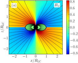
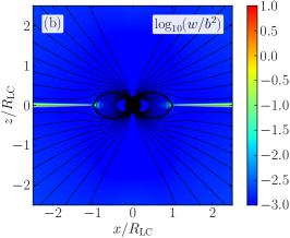
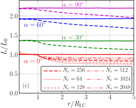
Figure 1: [Panels (a) and (b)] Meridional cut through a relativistic MHD magnetosphere of an aligned pulsar (model D0R2048) taken after $20$ rotations; by this time the shown part of the magnetosphere reached steady state. Solid lines show contours of enclosed magnetic flux which represent poloidal field lines. [Panel (a)] Colour shows out-of-plane magnetic field component, $B_{\otimes}$ (red/blue – pointing into/out of plane, see colour bar), associated with poloidal currents circulating in the magnetosphere. The boundary of the closed zone is shown with thick solid line. [Panel (b)] Colour shows the logarithm of the ratio of enthalpy, $w=\rho+\Gamma u_{g}$, to $b^{2}$ (red shows high and blue low values, see colour bar): $w/b^{2}$ is small near the star, where the magnetosphere is highly magnetized ($w/b^{2}\lesssim 10^{-3}$, the magnetization is about $10\times$ that in K06). However, $w/b^{2}$ exceeds unity in the equatorial current sheet, in which thermal pressure slows down plasma inflow and affects the velocity structure inside and near the sheet. [Panel (c)] Radial profiles of angle-integrated energy flux, $L$, normalized to $L_{0}$, the analytic approximation for the spin-down of an aligned rotator, see eq. (1): solid (dashed) lines show total (Poynting) energy flux. From bottom to top, models D0R64–D0R2048 (red), D30 (green), D60 (blue), D90 (magenta lines) are shown. For an aligned pulsar, Poynting fluxes at different resolutions are shown.

1 Introduction

The launch of the Fermi satellite opened a new window into studying the properties of pulsar magnetospheres, with more than $100$ $\gamma$-ray pulsars detected to date (Nolan et al., 2012). Since $\gamma$-ray emission can comprise a substantial ($\lesssim 10\%$) fraction of total pulsar spin-down losses, $\gamma$-ray production mechanism should be capable of efficiently converting magnetospheric electromagnetic energy into $\gamma$-ray radiation. Historically, much effort went into studying vacuum pulsar magnetospheres based on the analytic magnetic field solution by Deutsch (1955), even though it was realized early on that for pulsars, which are filled with abundant plasma (Goldreich & Julian, 1969), force-free approximation is a more appropriate framework. Force-free approximation accounts for magnetospheric charges and currents but neglects plasma inertia, which is appropriate in the limit of high magnetization of the plasma $\sigma\equiv b^{2}/4\pi\rho c^{2}\gg 1$, with $b$ and $\rho$ the proper magnetic field and density. In recent years, self-consistent force-free solutions of axisymmetric (Contopoulos, Kazanas & Fendt, 1999; Gruzinov, 2005; McKinney, 2006b; Timokhin, 2006; Parfrey, Beloborodov & Hui, 2012) and oblique (Spitkovsky 2006, S06 hereafter; Kalapotharakos & Contopoulos 2009; Li et al. 2012b; Pétri 2012b) pulsar magnetospheres were numerically obtained. They feature a magnetospheric current sheet that could be responsible for powering the observed $\gamma$-ray emission (e.g., Bai & Spitkovsky, 2010a, b; Pétri, 2012a; Arka & Dubus, 2013; Uzdensky & Spitkovsky, 2012).

Magnetohydrodynamic (MHD) approach has important advantages relative to force-free because it includes plasma inertia, pressure, and velocity component along the magnetic field, all of which are missing in the force-free model. This information is crucial for modeling current sheet physics and for constructing realistic $\gamma$-ray light curves. Thus MHD holds the key to understanding global structure, dissipation, and emission processes in pulsar magnetospheres. The first 2D MHD simulation of the aligned pulsar magnetosphere was presented by Komissarov (2006), K06 hereafter. In this Letter we extend this work and construct time-dependent 3D relativistic MHD models of both axisymmetric and oblique pulsar magnetospheres and make comparisons to force-free models. In §2 we describe our numerical method and problem setup, and in §3 we present our results on magnetospheric structure and compare it to the split-monopole wind that is often used to describe asymptotic structure of oblique pulsar magnetospheres.

2 Numerical Method and Problem Setup

Table 1: Model details: model name, pulsar obliquity angle ($\alpha$), simulation resolution (given as $N_{r}\times N_{\theta}\times N_{\varphi}$), final time of the simulation ($t_{f}$, measured in units of pulsar period, $P$), pulsar spindown luminosity ($L$, measured in units of aligned pulsar spindown luminosity, $L_{0}$, eq. 1), fraction of spindown luminosity dissipated in the inner wind zone, $r<5R_{\rm LC}$ ($\epsilon$).

Name	$\alpha\ [^{\circ}]$	Resolution	$t_{f}/P$	$L/L_{\rm aligned}$	$\epsilon\ [\%]$
Relativistic MHD models (with HARM):
D0R64	$0$	$64\times 32\times 1$	$33$	$0.929$	$28$
D0R128	$0$	$128\times 64\times 1$	$45$	$0.983$	$23$
D0	$0$	$256\times 128\times 1$	$63$	$1$	$17$
D0R512	$0$	$512\times 256\times 1$	$44$	$1$	$14$
D0R1024	$0$	$1024\times 512\times 1$	$45$	$0.994$	$11$
D0R2048	$0$	$2048\times 1024\times 1$	$22$	$0.988$	$8.7$
D15	$15$	$256\times 128\times 128$	$5.2$	$1.13$	$19$
D30	$30$	$256\times 128\times 128$	$5.1$	$1.36$	$17$
D45	$45$	$256\times 128\times 128$	$5.1$	$1.64$	$15$
D60R64	$60$	$64\times 32\times 32$	$4.8$	$1.92$	$27$
D60R128	$60$	$128\times 64\times 64$	$5.5$	$1.94$	$16$
D60	$60$	$256\times 128\times 128$	$3.3$	$1.92$	$13$
D60R512	$60$	$512\times 256\times 256$	$3.5$	$1.96$	$12$
D75	$75$	$256\times 128\times 128$	$2.9$	$2.14$	$12$
D90	$90$	$256\times 128\times 128$	$5$	$2.2$	$11$

Force-free models (with HARM):      D0R64ff $0$ $64\times 32\times 1$ $7.7$ $0.839$ $50$ D0R128ff $0$ $128\times 64\times 1$ $30$ $0.886$ $47$ D0ff $0$ $256\times 128\times 1$ $240$ $0.914$ $45$ D0R512ff $0$ $512\times 256\times 1$ $10$ $0.925$ $45$ D0R1024ff $0$ $1024\times 512\times 1$ $16$ $0.93$ $43$ D0R2048ff $0$ $2048\times 1024\times 1$ $13$ $0.932$ $43$ D30ff $30$ $256\times 128\times 128$ $6.9$ $1.27$ $23$ D60ff $60$ $256\times 128\times 128$ $7$ $1.83$ $5.8$ D90ff $90$ $256\times 128\times 128$ $7$ $2.11$ $2$

We use general relativistic MHD code HARM (Gammie et al., 2003; McKinney & Gammie, 2004) including recent improvements (Tchekhovskoy et al., 2007, 2011; McKinney & Blandford, 2009; McKinney et al., 2012). For direct comparison to previous studies, we neglect stellar gravity and carry out the simulations in flat space. We place the surface of the neutron star (NS) at $r_{*}=0.2R_{\rm LC}$, where $R_{\rm LC}=c/\Omega$ is light cylinder (LC) radius, $\Omega$ is pulsar angular frequency, and $P=2\pi/\Omega$ is the pulsar period. We use a spherical polar computational grid, $r$, $\theta$, $\varphi$, with $\theta=0$ along the rotation axis, $\vec{\Omega}$. We also make use of cylindrical radius, $R=r\sin\theta$. The grid extends from the NS surface, $r_{\rm in}=r_{*}=0.2R_{\rm LC}$, to $r_{\rm out}=200R_{\rm LC}$. Grid spacing is uniform in $\theta-$ and $\varphi-$directions. The spacing is logarithmic in the radial direction, $\Delta r/r={\rm constant}$, at $r\lesssim r_{0}=20R_{\rm LC}$, and becomes progressively sparse, $\Delta r/r\propto(\log r)^{3/4}$, at $r\gtrsim r_{0}$.

We initialize the simulations with a dipolar magnetic field of a dipole moment, $\vec{\mu}$, that makes an angle, $\alpha$, with the rotation axis, $\vec{\Omega}$. At the inner $r-$boundary (the stellar surface), we set the perpendicular (to the magnetic field) 3-velocity component, $\vec{v}_{\perp}$, to enforce stellar rotation, and set the parallel 3-velocity component to zero, $\vec{v}_{||}=0$. We apply at the outer $r-$boundary standard outflow boundary conditions (BCs), at $\theta-$boundaries transmissive polar BCs (McKinney et al., 2012), and at $\varphi$-boundaries periodic BCs.

In a typical pulsar the magnetization near the LC can be very high, $\sigma_{\rm LC}\sim 10^{4}$. In a dipolar field, quantities drop off rapidly with $r$: $\rho\propto b\propto\sigma\propto r^{-3}$. This is numerically challenging: to ensure force-free-like conditions at the LC, $\sigma_{\rm LC}\gg 1$, we must have a very high $\sigma$ near the star, $\sigma_{*}=(R_{\rm LC}/R_{*})^{3}\sigma_{\rm LC}\simeq 10^{2}\sigma_{\rm LC}$, i.e., much higher than $\sigma\sim 10^{2}$ that our code can handle at reasonable resolutions in 3D. For our simulations to closely resemble the actual pulsar magnetospheres, we ensure force-free-like conditions inside the LC by driving density, $\rho$, internal energy, $u_{g}$, and the spatial part of parallel 4-velocity, $u_{||}\equiv\gamma v_{||}\equiv(\vec{B}\cdot\vec{u})\,{\rm sign}(B_{r})/B^{2}$, to target values, $\rho_{t}=b^{2}/4\pi c^{2}\sigma_{t}$ (with $\sigma_{t}=50$ or $100$), $u_{g,t}=0.2\rho_{t}c^{2}$, and $u_{||,t}=0$. We do this by modifying the variables, $q=\{\rho,u_{g},u_{||}\}$, at the end of each time step via $q=q_{t}+(q-q_{t})\exp(-\kappa\Delta t/\tau)$, where $\kappa=\{\cos\theta_{m},\cos\theta_{m},1\}$, $\theta_{m}$ is the magnetic colatitude, $\Delta t$ is the time step. For the driving timescale, we choose $\tau=0$ at $r\leq r_{1}=0.5R_{\rm LC}$, $\tau=\tau_{0}(r-r_{1})(r_{2}-r_{*})/[(r_{2}-r_{1})(r_{2}-r)]$ at $r_{1}<r<r_{2}=R_{\rm LC}$, and $\tau=\infty$ at $r\geq r_{2}$, where $\tau_{0}=0.005P$ (see also K06).

3 Results

Figure 2: Slices through a relativistic MHD simulation of an oblique pulsar magnetosphere ($\alpha=60^{\circ}$, model D60) taken after $3$ rotations. See Supporting Information for movies. Solid lines show field lines as traced in the image plane. Panels (a) and (b) show slices in $\vec{\mu}{-}\vec{\Omega}$, or $x-z$, plane. [Panel (a)] Shows out-of-plane magnetic field component, $B_{\otimes}$ with colour (red – into plane, blue – out of plane). [Panel (b)] Shows quantity $\log_{10}(w/b^{2})$ in color. It is low near the star, indicating a highly magnetized flow, and high in the current sheet, indicating the importance of thermal pressure support. [Panel (c)] Runs of 4-velocity components vs. radius along the $y=z=0$ line for the simulation, showing the proper velocity, $u\equiv\gamma v$ (green solid), and its component parallel to the magnetic field, $u_{||}$ (dash-dotted cyan line), and for the analytic split-monopolar force-free solution the proper drift velocity, $u^{\rm ff,mono}\equiv\Omega R$ (dashed magenta line). The location and thickness of the current sheet, which is centered at $x\approx 2.2R_{\rm LC}$, is indicated by the yellow stripe. [Panels (d)–(f)] Show colour maps of $u$ in $3$ orthogonal slices (see legends). In the current sheet, which is the putative source of $\gamma$-ray photons, $u$ undergoes rapid changes that are caused by a reconnection-induced inflow into the sheet and that can affect directionality and beaming of emergent radiation (see the main text for details).

We carried out a number of simulations for different values of the magnetic dipole inclination angle relative to pulsar rotation axis, $\alpha$, from $0^{\circ}$ (aligned rotator) to $90^{\circ}$ (orthogonal rotator). We refer to these as models Dxx, where xx is $\alpha$ measured in degrees, see Table 2. We indicate resolution used in a model via a suffix “R” followed by the number of grid cells in the $r-$direction; we omit the suffix for our default choice, $N_{r}=256$. Our $\theta$-resolution is tied to $N_{r}$ via $N_{\theta}=0.5N_{r}$, so the aspect ratio of computational cells is about unity, $\Delta r:r\Delta\theta:r\Delta\varphi\approx 1:1:2$. For all MHD models we use an ideal gas equation of state, $p_{g}=(\Gamma-1)u_{g}$, with the polytropic index, $\Gamma=4/3$, appropriate for a relativistically hot pair plasma.

Figures 1(a),(b) show the structure of magnetic field and the ratio of gas enthalpy to magnetic energy in our highest resolution aligned model, D0R2048, which is a 2D simulation. Since our relativistic MHD models are highly magnetized, with magnetization inside the LC $\sigma_{t}=100\gg 1$ (§2), they display the same generic features as force-free models. The currents in the magnetosphere and in the equatorial sheet cause the magnetosphere to open up and form a radial Poynting-flux-dominated wind (e.g., Michel 1973). However, not all of this wind reaches infinity: part of it enters the current sheet and heats it, possibly causing the sheet to produce high-energy emission. Whereas force-free approximation neglects plasma thermal pressure, Fig. 1(b) demonstrates that in MHD current sheets are dominated by the plasma pressure.

We carried out simulations of aligned pulsar magnetospheres at different resolutions (the first $6$ models in Tab. 2), and red lines in Fig. 1(c) show their radial energy flux profiles. The total energy flux is essentially independent of resolution and distance, indicating that our results are numerically converged, and agrees to within $1\%$ with that in other works (Gruzinov 2005; K06; S06; McKinney 2006b),

$$L_{0}=\frac{\mu^{2}\Omega^{4}}{c^{3}}.$$ (1)

We quantify the amount of dissipation in the wind zone as a fraction of total energy flux dissipated in the interval $r<5R_{\rm LC}$ via $\epsilon=1-L_{\rm EM}(5R_{\rm LC})/L(R_{\rm LC}).$ Table 2 and Fig. 1(c) show that $\epsilon$ monotonically decreases with increasing resolution, $\epsilon\propto N_{r}^{-1/3}=(2N_{\theta})^{-1/3}$: our axisymmetric MHD magnetospheres asymptotically (in the limit of infinite resolution) become dissipationless. This is to be expected: the level of current sheet dissipation is controlled by the magnetospheric resistivity, which in our approach is determined by the numerical resolution (see also Lyutikov & McKinney 2011).

Our relativistic MHD magnetosphere is similar to the one obtained using the low-dissipation force-free code by S06: most of the field lines that cross the surface of LC open up to infinity, with only a small fraction of them entering the current sheet, where they dissipate a vanishingly small fraction of pulsar spindown energy. Note that due to high numerical dissipation, standard force-free codes often reach a very different solution: most poloidal magnetic field lines close through the midplane, where they dissipate most of pulsar spin-down energy. K06 noted this effect, and we do as well when we use the force-free version of HARM (McKinney, 2006a; Lyutikov & McKinney, 2011). Namely, we find very high levels of dissipation, $\epsilon\sim 50\%$, that do not decrease with increasing resolution (see Tab. 2). Such absence of decrease is unphysical: had the models included thermal pressure produced by current sheet dissipation, that pressure would have slowed down the inflow into the current sheet, suppressed the reconnection, and led to lower values of $\epsilon$ (K06). Recently, Gruzinov (2008, 2011a, 2011b, 2011c, 2012) considered resistive force-free simulations of pulsar magnetospheres and argued that the current sheet dissipates up to $50$% of pulsar spin-down energy and that an increase in resolution does not change the dissipation rate. Our results suggest that the results of Gruzinov (2008, 2011a, 2011b, 2011c, 2012) for axisymmetric pulsars are dominated by the large numerical resistivity of their numerical scheme and converge to the unphysical, dissipative force-free solution.

Why does the force-free HARM (McKinney 2006a, Lyutikov & McKinney 2011) and many other force-free codes (e.g., K06; Gruzinov 2011c, 2012; Pétri 2012b) show such high levels of dissipation? To handle discontinuities in the flow, force-free HARM uses a Lax-Friedrichs Riemann solver that is not specialized to treating current sheets and hence spreads the sheet over several grid cells. However, no force-balance inside the sheet is possible since in force-free there is no thermal pressure to slow down reconnecting fields. Unless one prescribes a zero velocity of inflow into the sheet (McKinney, 2006b), the lack of force-balance across the sheet in force-free causes rapid reconnection (K06). In contrast, the force-free scheme by S06 can treat current sheets as true unresolved discontinuities, so reconnection in the sheet is minimal. As evidenced by our MHD results, we believe that in the limit of low reconnection the low dissipation force-free solutions as in S06 are more representative of the physical pulsar magnetospheric shape than dissipative force-free solutions with uncontrolled numerical reconnection rate (e.g., Gruzinov, 2011c, 2012).

We now consider oblique models, applicable to the majority of pulsars. We present results for magnetization $\sigma_{t}=50$ (results at $\sigma_{t}=100$ are similar and not shown). Figure 2(a) shows the $\vec{\mu}{-}\vec{\Omega}$ plane for our oblique model D60: electromagnetic quantities in our relativistic MHD models reproduce, as expected, major features of oblique force-free solutions of pulsar magnetospheres (see Fig. 2(a) in S06), such as the formation of closed and open field line zones and the undulating equatorial current sheet. Please see Supporting Information for movies. Additionally, MHD models provide crucial information about plasma properties, e.g., velocity and temperature in the current sheet, which are needed for light curve computation but are missing from a force-free description. Although resistivity in our scheme is numerical, the reconnection displays physical characteristics. Fig. 2(b) shows that thermal and magnetic pressures are of the same order inside the current sheet, as in our axisymmetric models (see Fig. 1b). Hence, the thermal pressure is dynamically important in the current sheet and affects the fluid velocity there.

Figure 2(c) shows the radial dependence of velocity along the line $y=z=0$. Near the star the proper velocity, or spatial component of $4$-velocity, $u\equiv\gamma v$, follows the split-monopole force-free model of an oblique rotator (Bogovalov, 1999), $u^{\rm ff,mono}=\Omega R$ (e.g., Narayan et al., 2007). However, further out we clearly have $u>\Omega R$, followed by a sharp drop in $u$ across the sheet and $u<\Omega R$ on the other side of the sheet. This discontinuity in $u$, which naturally emerges due to a reconnection-induced inflow of fields and plasma into the sheet, is neglected in the split-monopole model. Inside the current sheet, the velocity components in the simulation appear to pass through the split-monopole values (e.g., $u=\Omega R$). This suggests that in a volume-averaged sense the split-monopole model might give a reasonable description of velocity in the current sheet even in the presence of reconnection. The lower row of panels in Fig. 2 shows three orthogonal cross-sections through our fiducial oblique model, D60. The discontinuity in $u$ is clearly co-spatial with the sheet. We find a similar behavior of velocity in our force-free HARM models, which reaffirms that qualitatively magnetospheric structure is insensitive to the microphysics of the model. At the stellar surface we assume that the plasma is at rest relative to the star and its proper velocity component parallel to the magnetic field vanishes, $u_{||}=0$. Unlike force-free, MHD allows us to compute $u_{||}$ self-consistently in the bulk of the flow. We find $u_{||}>0$, except near the current sheet, i.e., the plasma predominantly streams along magnetic field lines away from the star. However, since $u_{||}\ll u$, this streaming has negligible effect on plasma net velocity.

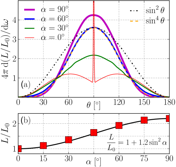
Figure 3: [Panel (a)] Lateral distribution of pulsar wind luminosity per unit solid angle, $dL/d\omega$, for models D0R2048, D30, D60, D90, as measured at $r=2R_{\rm LC}$. The spike at $\theta=90^{\circ}$ for D0R2048 model is due to kinetic+thermal energy outflow along the equatorial current sheet. At high ($\alpha\gtrsim 60^{\circ}$) obliquity pulsar wind luminosity is more equatorially concentrated (dashed line) than in the split-monopole wind model (dash-dotted line). [Panel (b)] Pulsar luminosity increases with increasing obliquity angle, $\alpha$, for our MHD models, D0–D90, in excellent agreement with S06.

Figure 1(c) shows the radial profiles of total and Poynting (electromagnetic) energy fluxes for models at different values of pulsar obliquity. The total energy flux, $L(r)$, is conserved to better than $3\%$ accuracy in all cases. We confirmed that our oblique models are numerically converged: an $8\times$ increase in resolution affects the spindown rate by $\leq 2\%$ (compare models D60R64, D60R128, D60 and D60R512 in Tab. 2). Based on this, we conservatively estimate that the accuracy of our spin down energy loss measurements is $\simeq 5\%$. Interestingly, Table 2 shows that changing resolution for our tilted model D60 leads to much smaller changes in the amount of magnetospheric dissipation, $\epsilon$, than in our axisymmetric models. This suggests that the 3D motion of the current sheet through the numerical grid increases the dissipation in our scheme.

Table 2 shows that the amount of magnetospheric dissipation in our force-free HARM models, D0ff-D90ff, dramatically decreases as inclination angle increases. Namely, dissipation is unacceptably high, $\epsilon\gtrsim 25\%$, at low inclination angles, $\alpha\lesssim 30^{\circ}$. However, the dissipation becomes much smaller, $\epsilon\lesssim 5\%$, at higher inclination angles, $\alpha\gtrsim 60^{\circ}$. This low level of magnetospheric dissipation (in fact, even smaller than in our MHD models) for highly inclined force-free HARM pulsars indicates that force-free HARM models D60ff and D90ff provide a good description of the electromagnetic part of pulsar magnetosphere. Our MHD models do not show such strong trends of $\epsilon$ vs. $\alpha$ and are applicable at all inclination angles. It is likely that the improved dissipation properties of force-free schemes at large inclinations have to do with the larger fraction of the current in the sheet that is carried by the displacement current for higher obliquity. Force-free schemes without conduction currents become vacuum-like in the sheet region, and this may suppress reconnection there. This is not the case for MHD schemes which still have to include the plasma in the current sheet.

It was suggested that aligned (Ingraham, 1973; Michel, 1974) and oblique (Bogovalov, 1999) pulsar magnetospheres resemble the split-monopole wind asymptotically far from the star. That the field lines in Figs. 1 and 2 are predominantly radial supports this suggestion. However, quantitatively, pulsar wind substantially differs from the split-monopole. As noted above, reconnection-induced inflow into the magnetospheric current sheet modifies the velocity of the wind. The lateral distribution of wind luminosity flux also deviates from split-monopole’s $dL/d\omega\propto\sin^{2}\theta$. For the aligned pulsar, instead of peaking at the equator, the wind luminosity is double-peaked (red line in Fig. 3a). For highly inclined pulsars, with $\alpha\gtrsim 60^{\circ}$, the wind luminosity is well-described by $dL/d\omega\propto\sin^{4}\theta$ (solid blue line and orange dashed line in Fig. 3a are on top of each other) and is thus substantially more equatorially-concentrated than the analytic split-monopole expectation, $dL/d\omega\propto\sin^{2}\theta$ (dot-dashed black line in Fig. 3b). This has potentially important consequences for the theoretical modeling of pulsar wind nebulae, where the angular distribution of wind luminosity can be directly observed. We confirmed the deviations from split-monopole using MHD and force-free versions of HARM, and with force-free code of S06.

Figure 3(b) shows that pulsars at high obliquity lose larger amounts of energy than at low obliquity. Both in our MHD and force-free HARM models the spin-down power, $L$, is well-described by the analytic fitting formula, $L/L_{0}=k_{1}(1+k_{2}\sin^{2}\alpha$), in good agreement with force-free results of S06, albeit with slightly different values of numerical factors, $k_{1}=1$ and $k_{2}=1.2$.

4 Conclusions

We obtained axisymmetric and oblique pulsar magnetosphere solutions using time-dependent relativistic MHD equations in 3D. We used a conservative relativistic MHD formulation that allowed us to account for resistive heating and thermal pressure support in magnetospheric current sheets, both of which are important for obtaining numerically converged solutions (see §3). Our solutions are highly magnetized, with $\sigma=b^{2}/4\pi\rho c^{2}\simeq 50{-}100$ near the LC, and are, therefore, close to force-free. We verified that the electromagnetic spin down power in our relativistic MHD models quantitatively agrees with force-free models. Our MHD models generalize force-free solutions by providing crucial information about fluid motions that is missing from a force-free description: plasma density, pressure, and the velocity component parallel to the magnetic field, $u_{||}$. Knowing this information is required for computing the beaming and phase of current sheet’s $\gamma$-ray emission (Bai & Spitkovsky, 2010a, b) either due to thermal or non-thermal particles (Arka & Dubus, 2013; Uzdensky & Spitkovsky, 2012). These calculations will be presented in an upcoming publication. We note that while MHD models provide a complete description of plasma motion along the open field lines, we still have to switch to a force-free-like description inside the LC to avoid mass and internal energy build-up on the closed field lines (see §2).

We showed that the conventional expectation that the magnetospheric structure is well-described by the split-monopole wind model does not hold quantitatively: at high inclinations, $\alpha\gtrsim 60^{\circ}$, the pulsar wind luminosity is more equatorially concentrated than in a split-monopole wind and the wind velocity structure is modified by reconnection-induced inflow into the magnetospheric current sheet. Our work considered a non-relativistic outflow from the surface of the NS ($u_{||}=0$). We plan to investigate if an ultra-relativistic outflow from the surface ($u_{||}\gg 1$) can cause ultra-relativistic velocity inside the current sheet on the scales of LC. As magnetospheric conductivity can vary, possibly influenced by the amount of magnetospheric plasma supply (Li et al., 2012a, b), resistive relativistic MHD codes should be developed (Komissarov, 2007; Palenzuela et al., 2009; Dionysopoulou et al., 2012) and used to study physical resistivity effects on the structure of magnetospheric current sheets and $\gamma$-ray light curves (Li et al., 2012a, b; Kalapotharakos et al., 2012a, b). This will also allow studies of plasma accumulation and plasmoid formation near the Y-point that can explain pulsar glitches and associated changes in pulsar braking indices (Contopoulos 2005; Bucciantini et al. 2006; S06).

Acknowledgments

AT is supported by the Princeton Center for Theoretical Science Fellowship. AS is supported by NSF grant AST-0807381 and NASA grants NNX09AT95G, NNX10A039G, NNX12AD01G. We thank the anonymous referee for insightful suggestions that helped improve the manuscript and Jonathan C. McKinney and Alexander Philippov for fruitful discussions. The simulations presented in this article used computational resources supported by the PICSciE-OIT High Performance Computing Center and Visualization Laboratory, and by XSEDE allocation TG-AST100040 on NICS Kraken and Nautilus and TACC Ranch.

Supporting Information

Additional Supporting Information is available for this article.
Movie files. Movies of model D60: movie 1 (link) and 2 (link).

References

- Arka & Dubus (2013) Arka I., Dubus G., 2013, A&A, 550, A101
- Bai & Spitkovsky (2010a) Bai X.-N., Spitkovsky A., 2010a, ApJ, 715, 1282
- Bai & Spitkovsky (2010b) Bai X.-N., Spitkovsky A., 2010b, ApJ, 715, 1270
- Bogovalov (1999) Bogovalov S. V., 1999, A&A, 349, 1017
- Bucciantini et al. (2006) Bucciantini N., et al., 2006, MNRAS, 368, 1717
- Contopoulos (2005) Contopoulos I., 2005, A&A, 442, 579
- Contopoulos et al. (1999) Contopoulos I., Kazanas D., Fendt C., 1999, ApJ, 511, 351
- Deutsch (1955) Deutsch A. J., 1955, Annales d’Astrophysique, 18, 1
- Dionysopoulou et al. (2012) Dionysopoulou K., Alic D., Palenzuela C., et al., 2012, ArXiv:1208.3487
- Gammie et al. (2003) Gammie C. F., McKinney J. C., Tóth G., 2003, ApJ, 589, 444
- Goldreich & Julian (1969) Goldreich P., Julian W. H., 1969, ApJ, 157, 869
- Gruzinov (2005) Gruzinov A., 2005, Physical Review Letters, 94, 021101
- Gruzinov (2008) Gruzinov A., 2008, J. Cosm. Astrop. Phys., 11, 2
- Gruzinov (2011a) Gruzinov A., 2011a, ArXiv:1111.3377
- Gruzinov (2011b) Gruzinov A., 2011b, ArXiv:1101.5844
- Gruzinov (2011c) Gruzinov A., 2011c, ArXiv:1101.3100
- Gruzinov (2012) Gruzinov A., 2012, ArXiv:1209.5121
- Ingraham (1973) Ingraham R. L., 1973, ApJ, 186, 625
- Kalapotharakos & Contopoulos (2009) Kalapotharakos C., Contopoulos I., 2009, A&A, 496, 495
- Kalapotharakos et al. (2012a) Kalapotharakos C., Harding A. K., Kazanas D., et al., 2012, ApJ, 754, L1
- Kalapotharakos et al. (2012b) Kalapotharakos C., Kazanas D., Harding A., et al., 2012, ApJ, 749, 2
- Komissarov (2006) Komissarov S. S., 2006, MNRAS, 367, 19
- Komissarov (2007) Komissarov S. S., 2007, MNRAS, 382, 995
- Li et al. (2012a) Li J., Spitkovsky A., Tchekhovskoy A., 2012a, ApJ, 746, L24
- Li et al. (2012b) Li J., Spitkovsky A., Tchekhovskoy A., 2012b, ApJ, 746, 60
- Lyutikov & McKinney (2011) Lyutikov M., McKinney J. C., 2011, Phys. Rev. D, 84, 084019
- McKinney (2006a) McKinney J. C., 2006a, MNRAS, 367, 1797
- McKinney (2006b) McKinney J. C., 2006b, MNRAS, 368, L30
- McKinney & Blandford (2009) McKinney J. C., Blandford R. D., 2009, MNRAS, 394, L126
- McKinney & Gammie (2004) McKinney J. C., Gammie C. F., 2004, ApJ, 611, 977
- McKinney et al. (2012) McKinney J. C., Tchekhovskoy A., Blandford R. D., 2012, MNRAS, 423, 3083
- Michel (1973) Michel F. C., 1973, ApJ, 180, L133
- Michel (1974) Michel F. C., 1974, ApJ, 187, 585
- Narayan et al. (2007) Narayan R., McKinney J. C., Farmer A. J., 2007, MNRAS, 375, 548
- Nolan et al. (2012) Nolan P. L., Abdo A. A., Ackermann M., et al., 2012, ApJS, 199, 31
- Palenzuela et al. (2009) Palenzuela C., Lehner L., Reula O., et al., 2009, MNRAS, 394, 1727
- Parfrey et al. (2012) Parfrey K., Beloborodov A. M., Hui L., 2012, MNRAS, 423, 1416
- Pétri (2012a) Pétri J., 2012a, MNRAS, 424, 2023
- Pétri (2012b) Pétri J., 2012b, MNRAS, 424, 605
- Spitkovsky (2006) Spitkovsky A., 2006, ApJ, 648, L51
- Tchekhovskoy et al. (2007) Tchekhovskoy A., McKinney J. C., Narayan R., 2007, MNRAS, 379, 469
- Tchekhovskoy et al. (2011) Tchekhovskoy A., Narayan R., McKinney J. C., 2011, MNRAS, 418, L79
- Timokhin (2006) Timokhin A. N., 2006, MNRAS, 368, 1055
- Uzdensky & Spitkovsky (2012) Uzdensky D. A., Spitkovsky A., 2012, ArXiv:1210.3346