A Pan-STARRS1 View of the Bifurcated Sagittarius Stream

Abstract

We use data from the Pan-STARRS1 survey to present a panoramic view of the Sagittarius tidal stream in the southern Galactic hemisphere. As a result of the extensive sky coverage of Pan-STARRS1, the southern stream is visible along more than $60^{\circ}$ of its orbit, nearly double the length seen by the SDSS. The recently discovered southern bifurcation of the stream is also apparent, with the fainter branch of the stream visible over at least $30^{\circ}$. Using a combination of fitting both the main sequence turn-off and the red clump, we measure the distance to both arms of the stream in the south. We find that the distances to the bright arm of the stream agree very well with the N-body models of Law & Majewski (2010). We also find that the faint arm lies ${\sim}5$ kpc closer to the Sun than the bright arm, similar to the behavior seen in the northern hemisphere.

1. Introduction

The past decade has seen a tremendous growth in the amount of known tidal substructure in the Galactic halo (Ibata et al., 2001; Newberg et al., 2002; Yanny et al., 2003; Martin et al., 2004; Grillmair & Dionatos, 2006; Grillmair, 2006; Belokurov et al., 2007b, a; Jurić et al., 2008). One of the most prominent and well-studied tidal streams in the halo is the Sagittarius stream. A wide variety of tracers have been used to study the stream, including main sequence turn-off (MSTO) stars (Belokurov et al., 2007a), blue horizontal branch (BHB) stars (Niederste-Ostholt et al., 2010; Ruhland et al., 2011), A stars (Yanny et al., 2000; Martínez-Delgado et al., 2001, 2004), M giants (Majewski et al., 2003), RR Lyrae (Vivas et al., 2001, 2005; Watkins et al., 2009) and red clump (RC) stars (Bellazzini et al., 2006; Correnti et al., 2010). These studies have all revealed that the Sgr stream is exceedingly complex and highly structured. The northern “bifurcation”, where the stream appears to split into two parallel streams, remains unexplained. Multiple possible causes of the bifurcation have been proposed (e.g., Fellhauer et al., 2006; Peñarrubia et al., 2010) but no explanation so far has proved satisfactory (e.g., Peñarrubia et al., 2011).

Recent work by Koposov et al. (2012) using the SDSS has shown that the Sgr stream is more complex than previously believed, with a bifurcation in the stream in the southern Galactic hemisphere as well as in the north. This has only added to the challenge of reconciling the diverse properties of the stream. It also changes the range of possible explanations, e.g., it is possible that each of the two northern streams comes from a different progenitor. As a result of all these features of the stream itself, along with uncertainties about the gravitational potential of the Galaxy (Helmi, 2004; Law et al., 2005; Johnston et al., 2005; Fellhauer et al., 2006), the Sgr stream has proven to be a serious challenge to any model that attempts to describe it. The model of Law & Majewski (2010) has been able to generally reproduce many of the features of the stream (assuming a triaxial Galactic potential), but the bifurcations are not yet accounted for.

These modeling challenges underscore the importance of obtaining a complete set of observations of the stream, including data from both the northern and southern Galactic hemispheres. In this work we focus on the southern component of the stream, using data from the Pan-STARRS1 project. Pan-STARRS’s extensive sky coverage allows for a comprehensive view over approximately $60^{\circ}$ along the southern stream, yielding a picture in the south comparable to that available in the north.

In this work we extend the coverage of the southern Sgr stream seen by Koposov et al. (2012) in SDSS, nearly doubling the length of the stream observed. We measure distances along the entire observed southern stream, using red clump (RC) stars and a direct calibration of the RC absolute magnitude from the Sgr dwarf itself. The red clump is an excellent distance indicator, since it occupies a narrow range of absolute magnitudes and is only weakly dependent on the parameters of the stellar population. However, the red clump is a relatively weak feature, and in faint systems it can be difficult to unambiguously identify without additional information. This is particularly true at low galactic latitudes where the large number of disk stars increases the difficulties of identification. To mitigate this problem, we take advantage of the fact that the main sequence turn-off (MSTO) of the Sgr stream is much more well populated and easily identifiable. The MSTO is not an ideal distance indicator itself, since it exhibits considerable variation in absolute magnitude with differences in the age and metallicity of the stellar population, but it does provide a reasonable estimate of the stream’s distance such that we can use it as an additional constraint on the position of the RC.

Our distance measurements are thus made with a two-step process, whereby we first fit the bright edge of the MSTO, which unambiguously detects the Sgr stream but does not yield a precise distance, then use that measurement to set the range of apparent magnitudes which we use for detecting the red clump. The red clump fit then yields a precise distance.

Towards this goal, we first present an overview of the PS1 survey in Section 2, and present the PS1 view of the southern Sgr stream, along with distance measurements, in Section 3. We discuss the results of those fits and their relation to other works in Section 4, and conclude in Section 5.

2. Observations and Data Processing

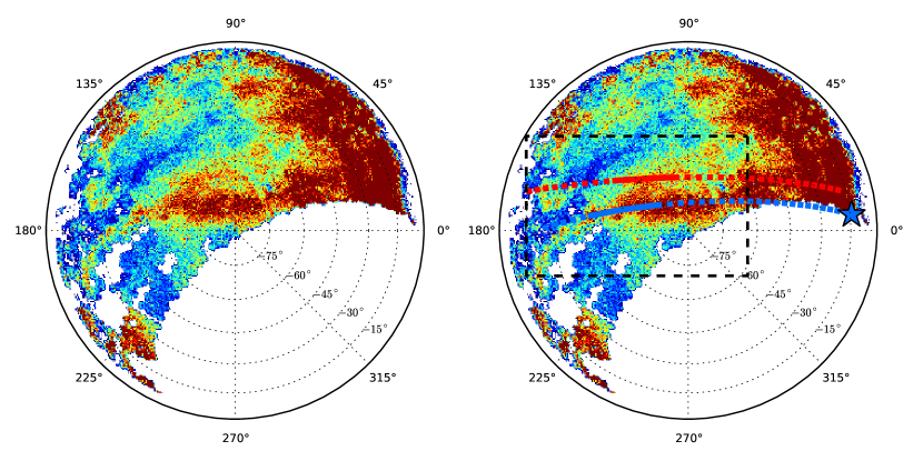
Figure 1.— Map of color-selected Sgr MSTO stars, shown in galactic coordinates and centered on the south galactic cap. The right image shows the position of the bright arm (solid blue) and the faint arm (solid red) as measured by Koposov et al. (2012), while the dashed versions show these lines extrapolated beyond the SDSS coverage. The position of the dwarf is indicated by the star on the right. The dashed rectangle indicates the region shown in Figure 2.

The observations were conducted by the Panoramic Survey Telescope and Rapid Response System 1 (Pan-STARRS1, hereafter referred to as PS1). PS1 is a 1.8m telescope on Haleakela, Maui, which has been conducting a multi-faceted survey since May 2010. The survey is designed both to detect transient, variable and moving objects, such as supernovae, Kuiper belt objects, asteroids, and stellar transits, and also to provide data to a number of static-sky projects, such as large scale structure, galaxy properties, and Milky Way structure. The survey covers the entire sky north of declination $-30^{\circ}$ (the so-called $3\pi$ survey), with 12 specific fields targeted for more frequent and deeper observations (the medium-deep survey).

The pattern of observations on the sky is organized by a fixed tessellation pattern which sets the boresight pointing locations. The timing of visits to each position is set by the need to obtain an adequate baseline in time for detection of transients and moving objects. The resulting set of observations for each position is designed to comprise of four observations of ${\sim}40$ seconds in each of the five PS1 filters, per observing season. The images are processed by the Pan-STARRS1 Image Processing Pipeline (IPP, Magnier, 2006), which handles all image processing steps including production of an object catalog for each image. Because of the computationally intensive nature of the processing on even single images, the IPP does not immediately produce stacked images. This is a necessary trade-off to enable the IPP to process images rapidly after the observations were taken, which is critical for the surveys of moving objects which require rapid follow-up observations.

As a result of this processing strategy, the currently available $3\pi$-survey catalogs contain only the results of photometry performed on single images. These catalogs are then cross-matched and merged to form an all-sky catalog. This does not increase the photometric depth in the same way that stacking images would, so it is not possible to detect objects fainter than the limiting magnitude of the deepest image. In order to reject spurious detections from instrumental artifacts we require that objects be detected multiple times, which makes our detection probability dependent on the number of visits to a position on the sky.

The depth of the resulting catalog is therefore dependent on the number and depth of individual exposures in each band in a particular region of the sky. The number of visits to each position on the sky varies due to weather and telescope downtime affecting the scheduling of visits. There are also variations in observing conditions between images, since the survey is designed to take data in marginal photometric conditions, which can affect the photometric completeness at faint magnitudes. To assess this variation, we have cross-matched the PS1 catalog with the SDSS “stripe 82” coadd catalog (Annis et al., 2011). The coadded SDSS catalog is better than 90% complete for stars down to 23rd magnitude in g, r, and i bands, so we can assume that the any non-detections of SDSS stars in the PS1 catalog is the result of PS1 incompleteness. From this cross-matching we can establish the 50% completeness magnitude over the range of observing conditions seen by the fields overlapping stripe 82. In g-band the 50% completeness ranges from approximately $g_{\rm P1}=21.4$ to $22.0$, in r-band from $r_{\rm P1}=21.2$ to $21.8$, and in i-band from $i_{\rm P1}=21.0$ to $21.8$. While these depths are fainter the range of magnitudes we use for in this work, because the completeness is not a step function as a function of magnitude there will be some variation in completeness even in the brighter data we use for the MSTO fitting. From this cross-matching we can see that the completeness at $i_{\rm P1}=21.0$ varies by approximately 20% across the range of observing conditions in stripe 82. This variation is reduced to 5% or less at magnitudes of $i_{\rm P1}=19.0$ or brighter. Much of this variation is likely to be related to our ability to separate stars from galaxies, which is progressively degraded under worse observing conditions. The photometric uncertainty on detected objects is less variable and frequently very small, on average ranging from 0.04 to 0.08 magnitudes near the MSTO (at approximately 21.5 mag in g and r filters), and less than 0.03 mag at RC magnitudes (in r and i filters).

One of the major challenges with any large survey is photometric calibration. The initial calibration of the IPP catalog is performed by referencing stars in each image to stars from the 2 Micron All Sky Survey (Skrutskie et al., 2006), which provides a consistent way of calibrating single images across the entire sky. However, now that the survey has obtained a sufficiently large set of observations with overlapping images, it is possible to self-consistently calibrate the survey using stars observed in multiple overlapping observations. Commonly called “übercalibration”, this calibration strategy was adopted by SDSS (Padmanabhan et al., 2008) and has been implemented for PS1 by Schlafly et al. (2012). Comparisons between SDSS and the übercalibrated PS1 data show that the resulting measurements agree to $<10$ mmag in the $g_{\rm P1}$, $r_{\rm P1}$, and $i_{\rm P1}$filters (Schlafly et al., 2012). This calibration is applied to the data using the Large Survey Database software (LSD, Jurić, in prep.), which provides a fast and scalable interface to the large volume of data required. Analysis of the calibrated data was also performed using LSD. All of the observations were extinction corrected and de-reddened using the reddening maps of Schlegel et al. (1998). We make use of all PS1 $3\pi$ data obtained through January 18, 2012, at which time the survey has imaged the entire $3\pi$ target area, though not always at the target photometric depth.

3. The PS1 view of the Sgr stream

Figure 1 shows a map of stars in the southern Galactic hemisphere with colors similar to that of the Sgr stream MSTO ($0.0<(g_{\rm P1}-r_{\rm P1})_{0}<0.4$ and $20.25<g_{{\rm P1},0}<22.10$). The Galactic center is on the right edge, and the anticenter is on the left. The map is most sensitive to MSTO stars at heliocentric distances between 25 and 45 kpc (assuming an old, metal poor population). The position of the bright arm of the stream is illustrated by the blue line on the right panel and the position of the faint arm (as measured by Koposov et al., 2012) is shown by the red line. The stream is clearly visible at $b<-60^{\circ}$, nearly passing through the south Galactic pole. Towards the Galactic center, the stream skirts the edge of the PS1 coverage and becomes lost in the higher density environment of the Galactic center. In the anticenter direction, a combination of varying observation depth and the increasing heliocentric distance of the stream makes it difficult to discern the stream at $b>-45^{\circ}$.

The Sgr stream in the southern hemisphere has also been seen in SDSS data (Koposov et al., 2012) over a somewhat smaller area. The SDSS and PS1 coverages are shown in Figure 2. Koposov et al. (2012) have also shown that the Sgr stream in the southern Galactic hemisphere is bifurcated in much the same way as the northern part of the stream. They show that the density of MSTO stars is asymmetric, with MSTO stars extending further perpendicular to the stream on the northern side (top of Figure 2) than the southern side. This is apparent in both the SDSS maps and the PS1 maps.

3.1. Distance Measurements

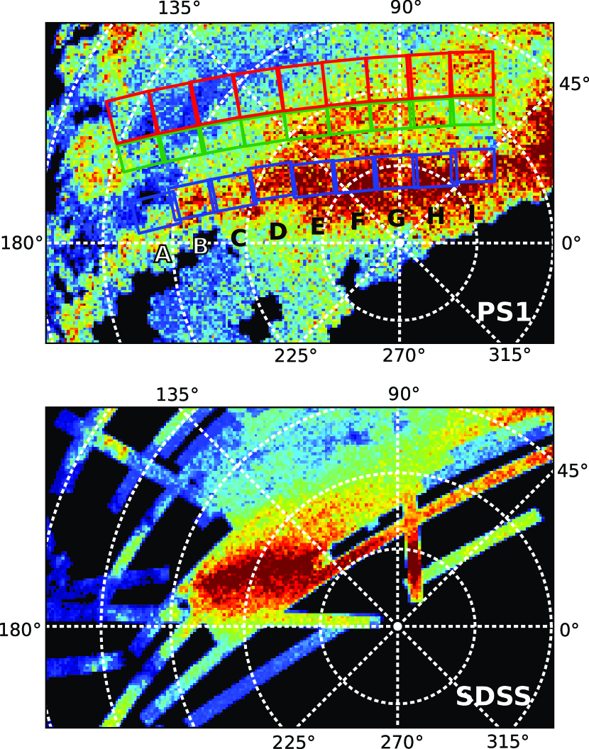
Figure 2.— Zoomed-in view of Figure 1, focusing on the Sgr stream. The top panel shows the data in PS1, while the bottom shows the same region in the SDSS. The top panel also shows the regions targeting the bright arm of the stream in blue, the faint arm regions in green, and the background regions in red. The coordinate grid labels show Galactic longitude, and the concentric rings are each separated by $15^{\circ}$ Galactic latitude.

We divide the length of the stream visible in the MSTO map into nine regions spaced equally along the Sgr plane defined by Majewski et al. (2003). Though this plane was designed to fit the position of the stream on the sky, the peak of the MSTO star density we observe lies slightly to the south of this plane. In order to improve the signal to noise of our measurements, for each of the nine regions we construct a histogram of MSTO star density as a function of distance off of the Sgr plane, then center our target on-source regions on the peak of these histograms. In general the region centers are approximately one degree south of the Sgr plane, but each region is fit individually so there is some variation. Not all of this variation is necessarily physical though, since we are also affected by small gaps in the PS1 sky coverage. As a result, the positions of these regions may only approximate the true position of the Sgr stream on the sky. The on-source regions cover $6^{\circ}$ along the stream and are $5^{\circ}$ wide perpendicular to the stream. The field centers are listed in Table 1, and the on-source regions are shown in the top panel of Figure 2 in blue.

In addition to placing on-source regions near the Sgr plane, we also placed regions $17^{\circ}$ away from the plane to serve as background regions for the MSTO fits. Ideally these background regions would be located at similar galactic latitude to the target regions, but at high galactic latitude the PS1 sky coverage does not include sufficient area that is not contaminated with the Sgr stream itself for this to be possible. Instead we adopted the strategy of background regions parallel to the stream, which for regions near the disk tends to approximate a constant galactic latitude selection process due to the position of the stream on the sky. At high galactic latitude this approximation begins to break down, but the background contamination is much less significant since those fields are far away from the disk. We also placed regions that targeted the faint arm of the stream approximately $10^{\circ}$ away from the plane, where the MSTO distribution shows a second peak or at least show signs of being spatially extended to the north. The resulting regions are shown in the top panel of Figure 2, with the faint arm regions in green and the background regions in red.

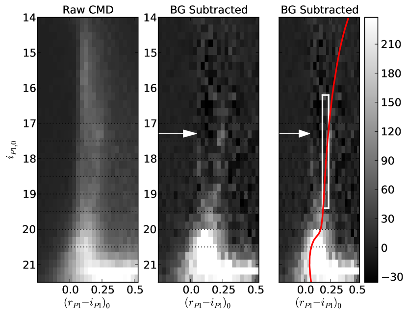
Figure 3.— CMDs for region E, showing the original on-source CMD (left), the background-subtracted CMD (center), and the background-subtracted CMD (right) with the RC color-cuts and an isochrone for an 11 Gyr old population with [Fe/H]$=-1.2$ overlaid (from Marigo et al., 2008). The horizontal arrow indicates the apparent magnitude of the red clump.

A background-subtracted color-magnitude diagram (CMD) for a sample region is shown in Figure 3. The background region was scaled to match the area of the target region. An isochrone of an 11 Gyr old population with [Fe/H]$=-1.2$ from Marigo et al. (2008) is shown for reference (computed with filter curves for the PS1 system; Tonry et al., 2012). This metallicity and age match measurements of the stream in the north, though the stream exhibits a broad range of metallicities (Chou et al., 2007). The Hess diagrams for the target fields were used to determine the color cuts that would best select the RC ($0.17<(r_{\rm P1}-i_{\rm P1})_{0}<0.23$) and the MSTO ($0.0<(r_{\rm P1}-i_{\rm P1})_{0}<0.10$). The RC color selection is shown by tall white rectangle.

These color cuts were then used to construct histograms of the apparent magnitudes of stars with the selected colors in each region. These regions are shown in Figure 4 for the bright arm regions and Figure 5 for the faint arm. For presentation purposes the figures show “running histograms”, similar to those used in Correnti et al. (2010) and Bellazzini et al. (2005). In these running histograms, each point is spaced by 0.02 magnitudes (the step size), but the value of each point is the number of stars within a 0.2 magnitude bin centered on the point (the bin size). The procedure is essentially a boxcar filter. The resulting step values are not statistically independent of each other, but the running histogram has the advantage that the visual appearance of the data is not affected by the particular bin positions in the histogram. That is, if the RC happens to fall on the edge between two bins of a conventional histogram, its signal appears more spread out than if it fell in the center of a single bin. The bin width is also chosen so that it roughly corresponds to the size of the RC, thus maximizing the signal to noise. The running histograms are primarily a presentation tool; all of the statistical fits which made use of histograms used “normal”, fixed-bin histograms.

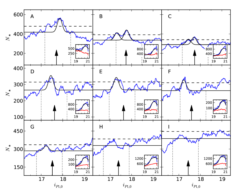
Figure 4.— Running histograms for the regions on the bright arm of the stream. The blue line shows the running histogram, while the black lines show the best fitting model (or multiple models in the case of multiple candidate peaks.) The horizontal dashed line indicates the level at which an overdensity would have a $3\sigma$ significance over the computed background level. The insets shows the MSTO fits used as a prior on the RC fits, with the on-stream data shown in blue, an off-stream background region shown in red, and the best fit model in black. The arrow shows the position of the red clump suggested by the MSTO fit, and the range of RC values allowed by the MSTO prior is shown by the vertical dotted lines. In cases where there was no peak with significance greater than 2-$\sigma$, we do not plot a fit and instead denote the background level with a solid horizontal line.

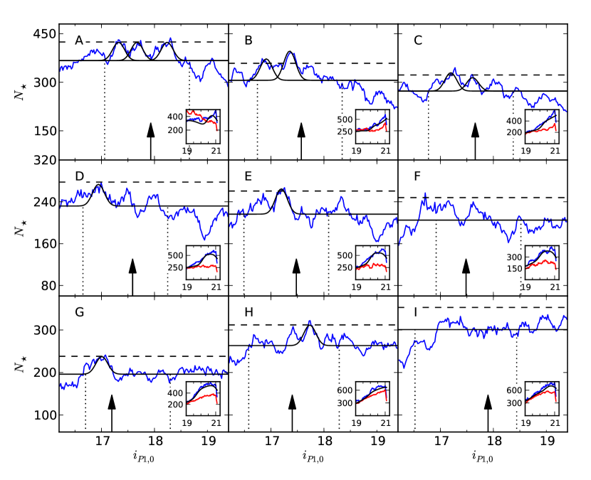
Figure 5.— RC fits for the regions placed on the faint arm of the stream. The lines are the same as in Figure 4. However, because we set the window for the bifurcation fits with the measured RC position in the on-stream regions, the allowed RC range (vertical dotted lines) may not align exactly with the center position suggested by the MSTO fit (vertical arrow).

3.1.1 MSTO Fit

After constructing the histograms of the MSTO and RC stars, we fit the apparent magnitude of the MSTO using a maximum likelihood method, modeling the edge of the MSTO as a step function superimposed on smooth background, as measured from the off-stream field and fit by a third-order polynomial. The step function was then convolved with a Gaussian with a width of $\sigma=0.10$ magnitudes to account for both photometric scatter and intrinsic scatter in the stellar luminosities. The result of these fits can be seen in the insets of Figure 4. In general these fits are very satisfactory, but it is clear that the edge of the MSTO is not a very sharp transition; the transition can span as much as half of a magnitude.

To use the MSTO fit as a prior on the RC fit, we must determine the difference in apparent magnitude between the two features. This calibration is inexact due to the various complicating factors associated with the MSTO but still yields useful results, since for this application we are only using it for different parts of the same stream. Since the composition of stellar populations in the stream is unlikely to vary greatly across the relatively modest length of stream available to us, the RC-MSTO offset should also only exhibit small variations. We computed this offset by creating synthetic CMDs from the Marigo et al. (2008) isochrones (using a Chabrier (2001) initial mass function), then applying the same color cuts and using the same maximum likelihood fits for the MSTO and RC position as were used on the PS1 data. Using an isochrone for an 11 Gyr old, [Fe/H]$=-1.2$ population the RC-MSTO offset was computed to be 2.50 magnitudes in i-band. Varying the metallicity of the isochrone from [Fe/H]$=-0.5$ to [Fe/H]$=-1.3$ (roughly the range of stream metallicities seen in the northern arm by Chou et al. (2007)) and also varying the age of isochrone from 6 Gyr to 11 Gyr, produced RC-MSTO offsets ranging from 2.71 through 2.40. The prior we adopt on the RC fit is therefore broader than this range of variation, but centered on an offset of 2.50 magnitudes.

3.1.2 RC Fit

A necessary step in fitting the RC is the determination of the smooth background level, which by number dominates over the RC. As shown in the CMD (Figure 3), the RC color cut we used is just slightly redder than the region of the CMD populated by nearby halo stars, which significantly outnumber the RC stars we are attempting to detect. Though the peak density of these stars occurs slightly bluer in color than the RC, both intrinsic scatter in color and photometric error causes some of these stars to fall into our color cuts. The apparent magnitude distribution of stars in this region of the CMD is approximately constant and not strongly affected by observing conditions. As a result, we model the RC background as a third order polynomial in color (between $(r_{\rm P1}-i_{\rm P1})_{0}=0.15$ and $0.35$) and a constant in apparent magnitude. The polynomial fitting excludes the RC color window to prevent biasing the background estimation.

This approach to modeling the background has a number of advantages. The primary reason for adopting this method is that the amount of background contamination to the RC color cut is highly sensitive to photometric errors in the observations. Greater observational uncertainties causes the large number of MSTO-color stars to occupy a wider range of colors, causing more to fall into the RC color cut and hence a higher background. This is particularly true for PS1, which has data spanning a range of observing conditions. This makes it very difficult to use off-stream regions as representative of the background level, since it is practically impossible to find suitable background regions that reproduce the observing conditions of an on-stream region. For this reason we also do not attempt to fit a precise function to the background as a function of apparent magnitude; though in several of the regions the background deviates from flatness, it generally does not do so in a way that could be modeled by comparison to an off-source region. Additionally, since our RC fits are constrained by the MSTO prior to a small range in apparent magnitude, it only matters that our background estimation matches that small part of the histogram well. The assumption of a constant background level is quite suitable under these conditions.

After we have obtained the prior on the RC fit from the MSTO, we fit to the data the sum of a Gaussian function with a fixed width of 0.1 magnitudes and the constant background level. The MSTO fit and the RC-MSTO calibration were used to set a flat prior within 0.6 mag of the center. The prior is broad enough to account for any variation in the age and metallicity of the stream, along with the inherent uncertainty and variability in the MSTO measurement as a result of observational factors. The scale factor on the Gaussian is then marginalized out, and the best fitting magnitude and uncertainty is found by taking moments of the likelihood. In general this produces good fits, with the statistical uncertainty in the measurement significantly smaller than the uncertainty of the RC calibration.

In a small number of fields, multiple distinct peaks appear in the histograms with significance greater than $3\sigma$. In many of these cases one of the peaks is more likely given the position of the stream in adjacent fields, but for completeness we report both distances. In some other fields, the RC appears to span a larger range of absolute magnitudes than expected, or exhibits some asymmetry that may indicate some feature is present other than the “pure” Sgr RC at a single distance. In these cases we do not have enough information to report multiple distances, since it would be an ambiguous exercise to decompose the noisy histogram into several RC components. Instead we report a single distance but with an uncertainty that reflects the entire range of magnitudes where the value of the running histogram exceeds the background by $3\sigma$, as estimated from pure Poisson noise (corresponding to the horizontal dashed lines in Figures 4 and 5). This effectively determines the range of magnitudes at which, if our assumption of a constant background holds, a statistically significant overdensity exists, even if we are unable to conclusively identify its origin.

An additional source of uncertainty comes from our assumption of the faint arm’s position on the sky. In selecting our regions for the distance measurements we have assumed that the faint arm parallels the bright arm over the region seen by PS1, but our MSTO maps are unable to localize the faint arm precisely enough to verify that this is the case. As shown by Koposov et al. (2012), the streams may be converging towards the Sgr dwarf at a rate of 0.05 degrees per degree along the stream. Our target regions are designed to be sufficiently wide perpendicular to the stream to encompass such gradients, but we have also tested our faint arm fits with the target regions placed along paths converging or diverging from the bright arm, with angles ranging from 0.10 deg/deg to -0.10 deg/deg. The results still generally agree well with the results from the parallel-stream assumption, but there is some variation in distances of approximately the same order or less than the uncertainties on individual distance measurements. As a result we have incorporated these additional uncertainties in our reported errors.

In order to use the RC as a distance indicator it is necessary to have a calibration of the feature’s absolute magnitude. This is complicated in the case of the RC by the fact that its absolute magnitude is weakly dependent on the age and metallicity of the stellar population (Seidel et al., 1987; Jimenez et al., 1998). These variations can be minimized by using a red photometric passband (Paczynski & Stanek, 1998) and by calibrating the RC magnitude with stars of the same stellar population at a known distance. This “differential” measurement was employed by Correnti et al. (2010) and is the method we use here. Since the Sgr dwarf lies within the PS1 survey area we are able to directly use the survey’s observations of the main body of the dwarf to calibrate our RC distance measurements along the stream. This avoids the need for any conversion between photometric systems. The histogram of RC color-selected stars in the main body of the dwarf is shown in Figure 6, in which the RC is immediately obvious. We fit the Sgr dwarf RC using the same methods as for the stream, but with a polynomial background measured from a neighboring off-source region instead of the constant used for the stream. The resulting fit measures the apparent magnitude of the RC to be $i_{\rm P1}=17.27\pm 0.05$. We adopt the Sgr dwarf distance measurement by Monaco et al. (2004), which used the tip of the red giant branch to measure a distance of $26.30\pm 1.8$ kpc, or a distance modulus of $(m-M)_{0}=17.10\pm 0.15$ (but see Kunder & Chaboyer (2009) for a recent alternative distance). All of our distance measurements are based on this number, and so all of our reported distances will scale directly with any revised value of the distance to the dwarf.

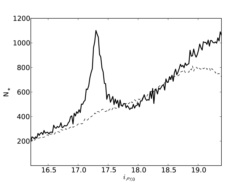
Figure 6.— Running histogram of RC color-selected stars in the main body of the Sgr dwarf. The solid line shows the histogram from the dwarf, while the dashed line shows the histogram for a background region.

4. Results & Discussion

Our measured distances to the stream are shown in Figure 7, with the bright arm shown in red points and the faint arm in blue. While the faint arm is just on the edge of detectability in several individual fields, the consistent behavior of the faint arm across the length of the stream does suggest that these detections do form a coherent structure. Despite the significant uncertainties on each individual measurement of the distance, the faint arm appears 3-5 kpc closer to the sun than the bright arm in several different fields. A distance offset between the two arms of the stream is also seen in the northern Galactic hemisphere, as seen by Yanny et al. (2009), Niederste-Ostholt et al. (2010), and Ruhland et al. (2011), where the faint arm (also called the “B” stream) also lies slightly closer to the sun than the bright stream (the “A” stream).

The distance to the main body of the trailing arm of the Sgr stream has also been measured with the red clump in SDSS data by Koposov et al. (2012). Their distances are shown in Figure 7 as the solid line. Comparing their results to ours for the bright arm of the stream, there is a clear difference of 7-10 kpc, which is consistent along the length of the stream. This appears to match our measured distances to the faint arm, but we believe that this is a coincidence. Koposov et al. (2012) show the density of RC stars along the stream in SDSS as a function of apparent magnitude (their Figure 5), and examination of this reveals that their detections of the RC lie at nearly the exact same apparent magnitudes as ours. However, Koposov et al. (2012) adopt an absolute magnitude of the RC as $M_{i}=0.6$, citing Bellazzini et al. (2006), while we use $M_{\rm i,PS}=0.17$ (the SDSS and PS1 i-band filters are nearly identical). This discrepancy is significantly larger than the uncertainty on the distance to the Sgr dwarf, which is 0.15 magnitudes. In Figure 7, the dashed line shows the distance measurements of Koposov et al. (2012) shifted by the difference between these calibrations, and the resulting distances agree well with our data. It thus appears that the discrepancy between the two results is caused by differences in the two RC absolute magnitude calibrations.

Though Koposov et al. (2012) refers to Bellazzini et al. (2006) as the source of their i-band RC calibration, it is unclear how this i-band measurement was obtained, since Bellazzini et al. (2006) uses observations performed entirely in the B and V bands and include no mention of the SDSS-i filter. With no further details provided by Koposov et al. (2012) we cannot diagnose the process that lead to this $M_{i}=0.6$ calibration. We are confident that our own calibration is robust: we detect the RC in the Sgr dwarf itself, using identical filters and observed as part of the same survey as our detections of the stream, thus minimizing the systematic uncertainty associated with color transformations and comparisons between data of different origins. One other possible source of variation between calibrations is the assumed extinction values to the Sgr dwarf, since it lies close to the Galactic plane, but it is unlikely that extinction could account for the magnitude of the calibration difference. Bellazzini et al. (2006) computes an average reddening of E(B-V)=0.116, while we use the value from the maps of Schlegel et al. (1998) which report E(B-V)=0.15. In terms of extinction this amounts to a difference in $A_{i}$ of 0.07 magnitudes, much less than the difference in the two calibrations.

In Figure 8, the measured distances are compared to the numerical model of the Sgr tidal streams produced by Law & Majewski (2010). The figure shows a projection of the stream onto the Galactic X-Z plane, which approximates the plane of the Sgr stream, and the Y-Z plane. The agreement between our distances and the position of the trailing (southern) arm of the Sgr debris is excellent. This is in light of the fact that the simulation was not selected to match the distance to the stream, but only the measured radial velocities to the leading and trailing streams. In the right panel of Figure 8, the Sgr dwarf appears slightly offset from the plane of the bright arm of the stream, but this is the result of a projection effect. Because the Sgr stream does not lie exactly in the X-Z plane, the projection of the stream onto the Y-Z plane will exhibit some variation in the Y direction. Because the dwarf lies on the opposite side of the Galactic center from the majority of the stream points, they will appear to be offset in Y when projected in this manner.

Figure 8 also shows the position of the Cetus stream, as measured by Newberg et al. (2009). Though the stream crosses the position of the Sgr stream on the sky, and in the X-Z plane of Figure 8 (left panel) appears to be coincident with detections of the faint arm, the X-Z projection of Figure 8 clearly shows that the Cetus stream passes behind the Sgr stream and not through it. It is therefore unlikely that our detections are confused with the Cetus structure.

Though there is currently no model for the origin of the northern and southern bifurcations that matches all of the available data, it is still instructive to examine how our results compare to the existing models in order to develop a sense of how a plausible bifurcation may behave in simulations. One hypothesis is that the Sgr dwarf was originally a disc galaxy, and that the material in the faint arm was stripped during a different pericentric passage than the bright arm (Peñarrubia et al., 2010). This theory is now thought to be untenable, since the Sgr dwarf is observed to have very little residual rotation (Peñarrubia et al., 2011), but the simulations used in Peñarrubia et al. (2010) are still useful for assessing the difficulty of reproducing the southern bifurcation simultaneously with the north. In the scenario that best reproduced the northern bifurcation, where the two streams are nearly coincident, the material from the two streams in the southern hemisphere is widely divergent. Material stripped in the same pericentric passage as the northern faint arm rapidly increases in helicentric distance towards the Galactic anticenter (from roughly 25kpc to 80kpc), while material from the bright arm stays at relatively constant heliocentric distance (from approximately 20kpc to 10kpc). These simulations were not designed to reproduce the stream’s behavior in the southern hemisphere and cannot be faulted for not doing so, but the discrepancy highlights the difficulty inherent in the problem.

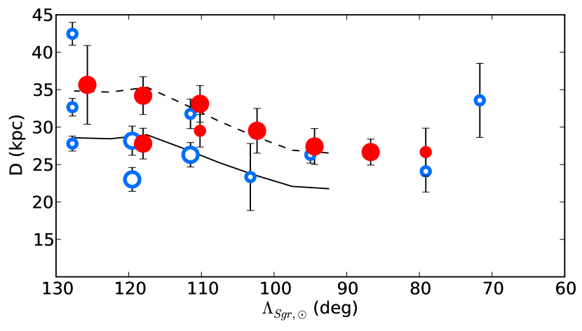
Figure 7.— Heliocentric distances to the bright arm (red, filled circles) and faint arm regions (blue, open circles), plotted in the Sgr coordinate system of Majewski et al. (2003). The smaller points indicate detections with significances between $2$ and $3\sigma$. The solid line indicates the distances to the Sgr stream reported by Koposov et al. (2012), while the dashed line shows the measurements of Koposov et al. (2012) but adjusted to our calibration of the RC absolute magnitude ($M_{i}=0.17$). The Sgr dwarf is located at $\Lambda_{Sgr,\odot}=0$.

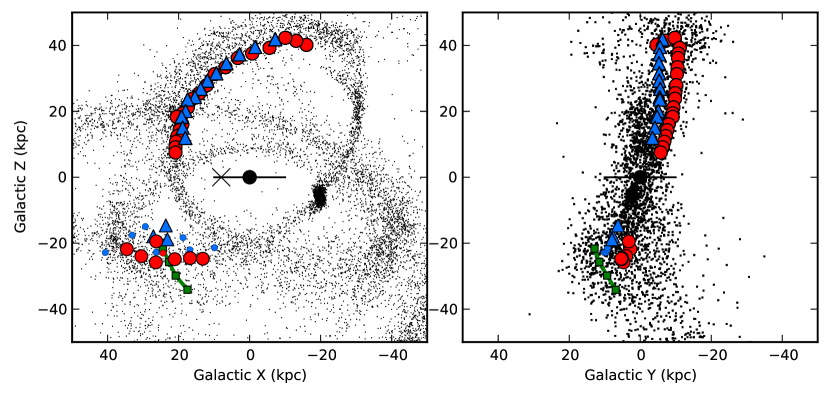
Figure 8.— Detected positions of the Sgr stream projected onto the Galactic X-Z plane (left), which approximates the orbital plane of the stream, and in the Y-Z plane (right), which is perpendicular to the orbit. The position of the Galactic disk is shown by the horizontal line, and the sun is marked with an $\times$. In the south, red circles and blue triangles signs indicate the position of statistically significant detections of the RC on the bright arm and the faint arm fields, respectively. The smaller points indicate detections with significances between $2$ and $3\sigma$. In the northern hemisphere, SDSS detections of the stream from Niederste-Ostholt et al. (2010) are shown with red circles for the bright arm, and blue triangles again for the faint arm. The position of the Cetus stream (Newberg et al., 2009) is also shown by the green squares. The black dots are data from the simulations of Law & Majewski (2010).

Field	A	B	C	D	E	F	G	H	I
Field center (RA,Dec)	(50,8)	(43,5)	(37,1)	(29,-2)	(23,-7)	(16,-11)	(9,-14)	(3,-18)	(356,-20)
Field center ($\Lambda_{sgr,\odot}$,$B_{sgr,\odot}$)	(126,-1)	(118,-1)	(110,-1)	(102,0)	(94,-0)	(87,-1)	(79,-1)	(72,-1)	(65,-0)
Distance (kpc)	35.6	34.2,27.8	33.1,29.5⁢*	29.5	27.4	26.7	26.7⁢*
Bifurcation center (RA,Dec)	(47,18)	(40,14)	(32,11)	(25,7)	(18,3)	(11,-1)	(4,-5)	(358,-8)	(351,-11)
Bifurcation center ($\Lambda_{sgr,\odot}$,$B_{sgr,\odot}$)	(128,9)	(120,9)	(112,10)	(103,10)	(95,10)	(87,10)	(79,10)	(72,10)	(64,10)
Bifurcation Distance (kpc)	42.5⁢*,27.8⁢*,32.7⁢*	28.2,23.0	26.3,31.8⁢*	23.3⁢*	26.3⁢*		24.1⁢*	33.6⁢*

Table 1 Positions of the regions along the Sgr stream used to detect the RC, along with the corresponding distance measurements. In cases where multiple overdensities could correspond to the red clump, the distances from each candidate position are listed. Detections with signifiance between $2$ and $3-\sigma$ are marked with an asterisk.

5. Conclusions

In this work we have used data from Pan-STARRS1 to show the spatial extent of the Sgr stream over $60^{\circ}$ of its orbit in the southern Galactic hemisphere. The position we observe of the stream on the sky matches well with observations from other surveys (Koposov et al., 2012) and with simulations (Law & Majewski, 2010). We have also shown that the stream in the southern hemisphere exhibits a bifurcation similar to that seen in the northern hemisphere, as was reported by Koposov et al. (2012).

Using a combination of the MSTO and the RC as distance indicators, we have measured the distance to both arms of the southern stream. Our results for the stream again agree well with the simulations of Law & Majewski (2010), but disagree with the distances measured by Koposov et al. (2012). We believe that this disagreement is the result of differences in calibrations of the RC absolute magnitude, and not differences between the SDSS and PS1 surveys, but it is not possible for us to further deduce the exact cause of the disagreement. Our calibration strategy, based on direct observations of the Sgr dwarf within the PS1 survey, gives us confidence that we have one of the most direct calibrations possible, free of any photometric transforms between data sources. Our distance measurements consistently place faint arm of the stream slightly closer in heliocentric distance than the bright arm. This is similar to the behavior seen in the northern hemisphere, again suggesting that the bifurcation is the result of some intrinsic behavior in the accreting Sgr system and not a coincidental overlap of multiple wraps.

Unfortunately there is no model for the bifurcation that can adequately explain the observed behavior. Models requiring multiple wraps of the stream (Fellhauer et al., 2006) or internal rotation of the Sgr dwarf appeared to be untenable even prior to the discovery of the bifurcation in the south (Yanny et al., 2009; Niederste-Ostholt et al., 2010). It has been speculatively suggested by Koposov et al. (2012) that what we call the Sgr stream could be the result of the accretion of a pair of dwarf galaxies simultaneously. Our observations should provide a quantitative basis against which simulations of a double accretion scenario can be tested. It is remarkable that one of the most prominent and most well-studied tidal streams has proven to be the most elusive streams to explain. While our observations can at the moment only deepen the mystery, we are hopeful that the added information on the stream’s behavior will be used to properly explain the bifurcation in future efforts.

References

- Annis et al. (2011) Annis, J., et al. 2011, ArXiv e-prints
- Bellazzini et al. (2005) Bellazzini, M., Gennari, N., & Ferraro, F. R. 2005, MNRAS, 360, 185
- Bellazzini et al. (2006) Bellazzini, M., Newberg, H. J., Correnti, M., Ferraro, F. R., & Monaco, L. 2006, A&A, 457, L21
- Belokurov et al. (2007a) Belokurov, V., et al. 2007a, ApJ, 658, 337
- Belokurov et al. (2007b) —. 2007b, ApJ, 657, L89
- Chabrier (2001) Chabrier, G. 2001, ApJ, 554, 1274
- Chou et al. (2007) Chou, M.-Y., et al. 2007, ApJ, 670, 346
- Correnti et al. (2010) Correnti, M., Bellazzini, M., Ibata, R. A., Ferraro, F. R., & Varghese, A. 2010, ApJ, 721, 329
- Fellhauer et al. (2006) Fellhauer, M., et al. 2006, ApJ, 651, 167
- Grillmair (2006) Grillmair, C. J. 2006, ApJ, 645, L37
- Grillmair & Dionatos (2006) Grillmair, C. J., & Dionatos, O. 2006, ApJ, 643, L17
- Helmi (2004) Helmi, A. 2004, ApJ, 610, L97
- Ibata et al. (2001) Ibata, R., Irwin, M., Lewis, G. F., & Stolte, A. 2001, ApJ, 547, L133
- Jimenez et al. (1998) Jimenez, R., Flynn, C., & Kotoneva, E. 1998, MNRAS, 299, 515
- Johnston et al. (2005) Johnston, K. V., Law, D. R., & Majewski, S. R. 2005, ApJ, 619, 800
- Jurić et al. (2008) Jurić, M., et al. 2008, ApJ, 673, 864
- Koposov et al. (2012) Koposov, S. E., et al. 2012, ApJ, 750, 80
- Kunder & Chaboyer (2009) Kunder, A., & Chaboyer, B. 2009, AJ, 137, 4478
- Law et al. (2005) Law, D. R., Johnston, K. V., & Majewski, S. R. 2005, ApJ, 619, 807
- Law & Majewski (2010) Law, D. R., & Majewski, S. R. 2010, ApJ, 714, 229
- Magnier (2006) Magnier, E. 2006, in The Advanced Maui Optical and Space Surveillance Technologies Conference
- Majewski et al. (2003) Majewski, S. R., Skrutskie, M. F., Weinberg, M. D., & Ostheimer, J. C. 2003, ApJ, 599, 1082
- Marigo et al. (2008) Marigo, P., Girardi, L., Bressan, A., Groenewegen, M. A. T., Silva, L., & Granato, G. L. 2008, A&A, 482, 883
- Martin et al. (2004) Martin, N. F., Ibata, R. A., Bellazzini, M., Irwin, M. J., Lewis, G. F., & Dehnen, W. 2004, MNRAS, 348, 12
- Martínez-Delgado et al. (2001) Martínez-Delgado, D., Aparicio, A., Gómez-Flechoso, M. Á., & Carrera, R. 2001, ApJ, 549, L199
- Martínez-Delgado et al. (2004) Martínez-Delgado, D., Gómez-Flechoso, M. Á., Aparicio, A., & Carrera, R. 2004, ApJ, 601, 242
- Monaco et al. (2004) Monaco, L., Bellazzini, M., Ferraro, F. R., & Pancino, E. 2004, MNRAS, 353, 874
- Newberg et al. (2009) Newberg, H. J., Yanny, B., & Willett, B. A. 2009, ApJ, 700, L61
- Newberg et al. (2002) Newberg, H. J., et al. 2002, ApJ, 569, 245
- Niederste-Ostholt et al. (2010) Niederste-Ostholt, M., Belokurov, V., Evans, N. W., & Peñarrubia, J. 2010, ApJ, 712, 516
- Paczynski & Stanek (1998) Paczynski, B., & Stanek, K. Z. 1998, ApJ, 494, L219
- Padmanabhan et al. (2008) Padmanabhan, N., et al. 2008, ApJ, 674, 1217
- Peñarrubia et al. (2010) Peñarrubia, J., Belokurov, V., Evans, N. W., Martínez-Delgado, D., Gilmore, G., Irwin, M., Niederste-Ostholt, M., & Zucker, D. B. 2010, MNRAS, 408, L26
- Peñarrubia et al. (2011) Peñarrubia, J., et al. 2011, ApJ, 727, L2
- Ruhland et al. (2011) Ruhland, C., Bell, E. F., Rix, H.-W., & Xue, X.-X. 2011, ApJ, 731, 119
- Schlafly et al. (2012) Schlafly, E. F., et al. 2012, ArXiv e-prints
- Schlegel et al. (1998) Schlegel, D. J., Finkbeiner, D. P., & Davis, M. 1998, ApJ, 500, 525
- Seidel et al. (1987) Seidel, E., Da Costa, G. S., & Demarque, P. 1987, ApJ, 313, 192
- Skrutskie et al. (2006) Skrutskie, M. F., et al. 2006, AJ, 131, 1163
- Tonry et al. (2012) Tonry, J. L., et al. 2012, ApJ, 750, 99
- Vivas et al. (2005) Vivas, A. K., Zinn, R., & Gallart, C. 2005, AJ, 129, 189
- Vivas et al. (2001) Vivas, A. K., et al. 2001, ApJ, 554, L33
- Watkins et al. (2009) Watkins, L. L., et al. 2009, MNRAS, 398, 1757
- Yanny et al. (2000) Yanny, B., et al. 2000, ApJ, 540, 825
- Yanny et al. (2003) —. 2003, ApJ, 588, 824
- Yanny et al. (2009) —. 2009, ApJ, 700, 1282