Time Dependent Radiative Transfer for Multi-Level Atoms using Accelerated Lambda Iteration

Abstract

We present a general formalism for computing self-consistent, numerical solutions to the time-dependent radiative transfer equation in low velocity, multi-level ions undergoing radiative interactions. Recent studies of time-dependent radiative transfer have focused on radiation hydrodynamic and magnetohydrodynamic effects without lines, or have solved time-independent equations for the radiation field simultaneously with time-dependent equations for the state of the medium. In this paper, we provide a fully time-dependent numerical solution to the radiative transfer and atomic rate equations for a medium irradiated by an external source of photons. We use Accelerated Lambda Iteration to achieve convergence of the radiation field and atomic states. We perform calculations for a three-level atomic model that illustrates important time-dependent effects. We demonstrate that our method provides an efficient, accurate solution to the time-dependent radiative transfer problem. Finally, we characterize astrophysical scenarios in which we expect our solutions to be important.

1 Introduction

The treatment of radiation transfer in complex, dynamic physical systems is crucial for theoretical modelling in a wide variety of astrophysical contexts. In this paper, we explore time-dependent effects in line transfer for low velocity media illuminated by external sources. Examples of such systems are found in absorbing material irradiated by light from gamma-ray bursts (GRBs) and active galactic nuclei (AGNs). In absorbing media, external photons enter at the boundary of the system, and are subsequently redistributed in angle and frequency by atomic interactions in the interior. This leads to a complicated, time-dependent coupling of the radiation field and the state of the medium.

Previous studies have investigated time-dependent radiative transfer in a number of regimes, under different approximations. Several papers have explored steady-state, non-LTE solutions to the radiative transfer equation (RTE) for time-dependent media. These works were done in the contexts of magnetohydrodynamics (e.g., Hayek et al., 2010; Davis et al., 2012), radiation hydrodynamics (e.g., Krumholz et al., 2012), smoothed particle hydrodynamics (e.g., Rundle et al., 2010), transport of cosmological ionization fronts (e.g., Whalen & Norman, 2006), molecular bands in planetary atmospheres (e.g., Kutepov et al., 1991), line transfer in stellar atmospheres (e.g., Sellmaier et al., 1993), multi-level transfer in moving media (e.g., Hauschildt, 1993; Harper, 1994), atmospheres of hot stars (e.g., Hubeny & Lanz, 1995), clumpy molecular clouds (e.g., Juvela, 1997), and line emission from interstellar clouds (e.g., Juvela & Padoan, 2005).

A few authors have investigated solutions to the time-dependent radiative transfer equation (TDRTE). Perna & Lazzati (2002) and Perna et al. (2003) treated time-dependent radiative transfer in static, dusty media in the optically thin limit, without radiation source terms. Gnedin & Abel 2001 and Abel & Wandelt 2002 also solved the time-dependent radiative transfer equation for cosmological reionization, neglecting photon scattering. Mihalas & Klein (1982) developed a ‘mixed-frame’ formalism for solving the time-dependent equations in the context of fluid flow, and investigated numerical methods for their solution. Kunasz (1983) calculated the numerical solution to the time-dependent transfer equation for resonance scattering in a static medium consisting of two-level atoms.

Recently, Hubeny & Burrows (2007) produced a self-consistent solution to the TDRTE for a time-dependent, non-LTE medium in radiation hydrodynamics. Their calculation focused on the propagation of neutrinos in supernova explosions, and did not explicitly treat line transfer of photons (see also Abdikamalov et al., 2012, for further discussion of time-dependent neutrino radiation transport).

In this paper, we neglect fluid flow, and focus instead on time-dependent effects in the line transfer of photons. In externally driven absorbing material, the time derivative of the RTE cannot be neglected due to the variability of the incoming radiation at the boundary of the system. The resulting solution depends on several crucial timescales: the variability timescale of the external source, $T_{\rm VR}$; the time interval between characteristic radiative interactions, $T_{\rm ref}$; and the light travel time across the width of the medium, $T_{\rm LC}$. For optically thick systems, $T_{\rm ref}\ll T_{\rm LC}$. If $T_{\rm VR}\ll T_{\rm ref}$, we argue that the source term for atomic interactions is unimportant for solving the TDRTE, and a simple, approximate solution is appropriate. Conversely, if $T_{\rm VR}\gg T_{\rm LC}$, then the RTE can be solved in steady-state, while the medium is treated as time-dependent; this situation has been discussed exhaustively in the literature. Thus, we are primarily interested in the ‘intermediate regime’, $T_{\rm VR}\gtrsim T_{\rm ref}$, $T_{\rm VR}\lesssim T_{\rm LC}$, and will perform a detailed analysis of this scenario in the work that follows.

The solution to the non-LTE radiative transfer problem has an enormous associated literature, a proper review of which is beyond the scope of this paper. In the work that follows, we extend the Accelerated Lambda Iteration (ALI) method to the case of time-dependent radiative transfer and atomic rate equations. The ALI approach employs a computationally inexpensive approximation to the RTE formal solution in the rate equations for the atomic level populations. This technique has its origins in the ‘core saturation’ method of Rybicki (1972, 1984), and Cannon’s operator splitting procedure (Cannon, 1973). Olson et al. (1986) showed that the diagonal part of the operator characterizing the formal solution to the RTE provides an efficient approximate operator for implementing ALI. Subsequently, Rybicki & Hummer (1991, 1992) developed a powerful formalism for applying ALI to non-LTE problems with multi-level atomic models. For a detailed review of ALI, see Hubeny (2003).

In this paper, we extend the TDRTE solution of Kunasz (1983) to time-dependent media with multi-level atoms, making extensive use of the Rybicki & Hummer (1992) formalism. To date, we have found no previous work in the literature that treats both the RTE and atomic rate equations as time variable for multi-level line transfer. Our method applies to general atomic models, including bound-bound and bound-free radiative transitions, collisional interactions, electron scattering, and background processes such as free-free absorption and emission. We present calculations for a specific three-level atomic model that illustrates important time-dependent radiative transfer effects. We find that these effects are important for systems in the intermediate regime and show that the use of approximate solutions that neglect them can lead to significant errors when interpreting spectroscopic observations. We consider the implications of our results for astrophysical systems, and provide a set of criteria for determining when the use of our formalism is necessary.

Our paper has the following outline: in §2, we describe our models for the atomic physics and external radiation sources used in our calculations; in §3, we review the basic equations for the TDRTE and atomic rate equations; in §4, we develop a general formalism for implementing the ALI solution; in §5, we show the results of our calculations; and in §6, we discuss implications of our results for astrophysical systems. In Appendix A, we extend our technique to include implicit Runge-Kutta time integration of our equations.

2 Models for Atomic Physics and External Radiation

We consider a plane parallel, finite slab of material that is illuminated by an external source of unpolarized radiation. The properties of the medium vary along the $z$ axis. The cosine of the polar angle, $\theta$, measured from the $z$ axis, is denoted by $\mu$. The system is assumed to be symmetric in the azimuthal direction.

The external radiation propagates toward the slab with $\theta>\pi/2$, reaching the medium at an arbitrary coordinate, $z_{\rm o}$. The width of the slab along the $z$ direction is denoted by $W$; thus, radiation exits the slab at $z_{\rm min}=z_{\rm o}-W$. After interacting with the medium, the radiation field in the slab consists of rays with $-\pi\leq\theta\leq\pi$. We assume that an observer is positioned in the $\theta=\pi$ direction.

To illustrate key properties of the time-dependent solutions, we perform calculations for a specific three-level atomic model. The atomic levels are labelled by $j=0,1,2$, and are connected by bound-bound radiative transitions between $j=0\leftrightarrow 1$, $j=0\leftrightarrow 2$, and $j=1\leftrightarrow 2$. We neglect other types of radiative and collisional interactions in our calculations, though they are straightforwardly included in our formalism, which is completely general.

The number density of the atoms is denoted by $n_{\rm o}$. We define a reference transition for photoexcitation between the atomic levels $j=0\rightarrow 2$, at line centre, with all atoms in the ground state. If the Einstein coefficient for this transition is $B_{02}$, and the line profile is due to Doppler broadening in complete redistribution, we obtain a reference extinction coefficient,

$$\chi_{\rm ref}=\frac{hB_{02}n_{\rm o}}{4\pi^{3/2}b/c},$$ (1)

where $b=\sqrt{2k_{B}T_{a}/m_{a}}$ is the Doppler width for an atom with temperature $T_{a}$ and mass $m_{a}$ (ignoring possible effects of microturbulence). We define a reference optical depth,

$$d\tau\equiv-\chi_{\rm ref}dz,$$ (2)

such that $\tau(z_{\rm o})=0$, and the maximum optical depth is $\tau(z_{\rm min})\equiv\tau_{\rm max}=\chi_{\rm ref}W$. We note that our definitions of $z$ and $\tau$ are opposite to those used in the stellar atmospheres literature, in which the optical depth increases with distance from the observer.

If we define a reference time,

$$T_{\rm ref}\equiv\left(c\chi_{\rm ref}\right)^{-1},$$ (3)

then the light crossing time for radiation passing through the slab is

$$T_{\rm LC}=W/c=\tau_{\rm max}T_{\rm ref}.$$ (4)

A natural unit of radiation intensity can be defined by equating the inverse of the photoexcitation rate for white, isotropic radiation exciting the reference transition, to the reference time:

$$I_{\rm o}\equiv c\chi_{\rm ref}/B_{02}.$$ (5)

When the photoexcitation rate for the reference transition is equal to $B_{02}I_{\rm o}$, the number density of line centre photons is equal to $n_{\rm o}$.

The Einstein coefficients for the transitions in our atomic model, using the units described above, are summarized in Table 1.

Table 1: Einstein coefficients for the transitions in our atomic model. $A$, $B_{\rm ex}$, and $B_{\rm em}$ are the coefficients for spontaneous emission, photoexcitation, and stimulated emission, respectively.

Transition	$A/T_{\rm ref}^{-1}$	$B_{\rm ex}/B_{02}$	$B_{\rm em}/B_{02}$
$0\rightarrow 2$	$1.4\times 10^{10}$	1	1.25
$1\rightarrow 2$	$4.9\times 10^{9}$	0.44	0.44
$0\rightarrow 1$	0.18	$1.7\times 10^{-5}$	$2.1\times 10^{-5}$

The values of the coefficients have been chosen so that the atomic model contains a resonance line ($j=0\leftrightarrow 2$), a strong transition between the excited states ($j=1\leftrightarrow 2$), and a weak transition between the ground and first excited states ($j=0\leftrightarrow 1$). This arrangement insures that the second excited state ($j=2$) remains relatively unpopulated, while the transition $j=0\rightarrow 2\rightarrow 1$ provides an efficient mechanism for populating the first excited state.

In §4, to make comparisons to the previous work of Kunasz (1983), we also consider a restricted version of the atomic model that includes only the single transition $j=0\rightarrow 2$.

For the calculations in this paper, we consider several basic models for the external radiation arriving at $\tau=0$. We assume that the angular variation of the incident radiation is either isotropic or highly collimated at the $\tau=0$ boundary of the slab. In the latter case, photons arrive from the external source in a narrow range of angles around the line of sight. In both cases, the spectrum of the external radiation is assumed to be white across all three atomic transitions.

We employ a heuristic model for the time variation of the arriving photons. This model combines a transient increase in intensity with a constant background intensity:

$$I_{\nu}^{\rm ext}(t,\mu)=\left\{I_{\rm B}+A\exp\left[-\frac{1}{2}\log^{2}\left(t/t_{0}\right)/\sigma^{2}\right]\right\}f(\mu),$$ (6)

where $I_{\nu}^{\rm ext}$ is the specific intensity of the incident radiation at $\tau=0$, $I_{\rm B}$ is a constant background intensity, and $A$ is the amplitude of the transient part of the incoming radiation. The variable part of equation (6) is a Gaussian pulse in $\log t$, where the parameters $t_{0}$ and $\sigma$ determine the centring and width of the pulse, respectively. The angular variation $f(\mu)$ is set to unity for isotropic sources, and takes the value $f(\mu)=\delta(\mu+1)$ for collimated sources. Thus, if $A\gg I_{\rm B}$, the external source emits photons in a transient pulse, whereas if $A\gtrsim I_{\rm B}$, the external radiation represents a persistent source with superimposed variability.

To make comparisons to the previous work of Kunasz (1983), we also employ a simple ‘ramp’ model in which the external source increases linearly from zero at $t/T_{\rm ref}=0$ to $I_{\rm B}$ over the time interval $10^{-2}T_{\rm ref}$, remaining constant thereafter.

3 Fundamental Equations

3.1 Radiative Transfer Equation

We restrict the range of angular values to $\mu\in[0,1]$, and write the specific intensity for the unpolarized radiation field as two distinct functions, $I_{\nu}^{+}(t,z,\mu)$ for $\theta\leq\pi/2$ and $I_{\nu}^{-}(t,z,\mu)$ for $\theta>\pi/2$. With this notation, the TDRTE can be written:

$$\frac{1}{c}\frac{\partial I_{\nu}^{\pm}}{\partial t}\pm\mu\frac{\partial I_{\nu}^{\pm}}{\partial z}=-\chi_{\nu}I_{\nu}^{\pm}+\eta_{\nu}.$$ (7)

The extinction and emission coefficients can be cast in a general form for bound-bound and bound-free radiative interactions (c.f., Rybicki & Hummer, 1992). We denote the frequency-angle rate coefficient for spontaneous emission or radiative recombination as $U_{lj}$, depending on whether $l\rightarrow j$ represents a bound-bound or bound-free transition. Note that $U_{lj}=0$ if $l\leq j$. Similarly, $V_{lj}$ denotes stimulated emission or recombination for $l>j$, and absorption or photoionization for $l<j$. For the familiar case of bound-bound transitions with complete redistribution in the line profile, the rate coefficients become:

$$U_{lj} =\left\{\begin{aligned} \frac{h\nu_{lj}}{4\pi}A_{lj}\varphi_{lj},&\quad l>j\\ 0,&\quad l<j\end{aligned}\right.$$ (8)

$$V_{lj} =\frac{h\nu_{lj}}{4\pi}B_{lj}\varphi_{lj},$$ (9)

where $\nu_{lj}$ is the line centre frequency of the transition, and $\varphi_{lj}$ is the absorption line profile. Note that under the assumption of complete redistribution, $\varphi_{lj}=\varphi_{jl}$. Similar equations can be written for bound-free interactions, or for different approximations for the redistribution of the line profile (see, e.g., Rybicki & Hummer, 1992; Uitenbroek, 2001). In this notation, the extinction and emission coefficients become:

$$\chi_{\nu} =\sum_{l,j;\,l<j}\chi_{lj}+\chi_{\rm c},$$ (10)

$$\eta_{\nu} =\sum_{l,j}U_{lj}n_{l}+\eta_{c},$$ (11)

where

$$\chi_{lj}\equiv V_{lj}n_{l}-V_{jl}n_{j},$$ (12)

and $\chi_{c}$, $\eta_{c}$ represent background processes or electron scattering; these contributions are treated separately in the numerical method from the bound-bound and bound-free interactions (see §4). The $\Sigma$ symbols in equations (10) and (11) denote double sums over the $j$ and $l$ indices for all transitions satisfying the indicated condition. The number density of atoms in level $l$ is denoted by $n_{l}$.

Equation (7) must be supplemented by initial and boundary conditions for the specific intensity in each angular range. The boundary conditions take the form:

$$I_{\nu}^{-}\left(t,z_{\rm o},\mu\right)=I_{\nu}^{\rm ext}(t,\mu),$$ (13)

$$I_{\nu}^{+}\left(t,z_{\rm min},\mu\right)=0.$$ (14)

The initial conditions are determined by solving the time independent radiative transfer equation (TIRTE), which is obtained by setting $\partial I_{\nu}^{\pm}/\partial t\rightarrow 0$ in equation (7). Equations (13) and (14), evaluated at $t/T_{\rm ref}=0$, are then used as boundary conditions for the TIRTE. The resulting solution is used for the initial conditions, $I_{\nu}^{\pm}(t=0,z,\mu)$. The TIRTE can be solved with an approach that is similar to the time-dependent method (see §4).

In developing numerical methods for solving the RTE, it is useful to define the Feautrier variables (see, e.g., Mihalas, 1978, and the references therein):

$$u_{\nu} =\left(I_{\nu}^{+}+I_{\nu}^{-}\right)/2,$$ (15)

$$v_{\nu} =\left(I_{\nu}^{+}-I_{\nu}^{-}\right)/2.$$ (16)

We define the optical depth along a ray path as:

$$d\tau_{\nu}=-\chi_{\nu}dz/\mu,$$ (17)

where $\tau_{\nu}(z_{\rm o})=0$. A change in variables to $u_{\nu}$, $v_{\nu}$, and $\tau_{\nu}$, results in the following form for the transfer equations:

$$\frac{\partial u_{\nu}}{\partial t} =c\chi_{\nu}\left(\frac{\partial v_{\nu}}{\partial\tau_{\nu}}-u_{\nu}+S_{\nu}\right),$$ (18)

$$\frac{\partial v_{\nu}}{\partial t} =c\chi_{\nu}\left(\frac{\partial u_{\nu}}{\partial\tau_{\nu}}-v_{\nu}\right),$$ (19)

where $S_{\nu}=\eta_{\nu}/\chi_{\nu}$ is the source function. Similarly, the boundary conditions can be rewritten as:

$$u_{\nu}(t,z_{\rm o},\mu)=v_{\nu}(t,z_{\rm o},\mu)+I_{\nu}^{\rm ext}(t,\mu),$$ (20)

$$u_{\nu}(t,z_{\rm min},\mu)=-v_{\nu}(t,z_{\rm min},\mu).$$ (21)

Equations (18) and (19), along with the boundary conditions (20) and (21), form the basis of our numerical solution to the RTE.

3.2 Atomic Rate Equations

The extinction and emission coefficients for the radiation field depend directly on the level populations of the various bound atomic states, as well as the degree of ionization of the medium. The rate equation for each level $j$ can be written:

$$\frac{dn_{j}}{dt}=\sum_{l}\Bigl{[}\left(C_{lj}+R_{lj}\right)n_{l}-\left(C_{jl}+R_{jl}\right)n_{j}\Bigr{]},$$ (22)

where $R_{lj}$ and $C_{lj}$ are the rate coefficients for radiative and collisional transitions between levels $l\rightarrow j$, respectively. The sum $\Sigma_{l}$ is over all atomic levels $l\neq j$. Using the notation of §3.1, we write the radiative rates as:

$$\begin{split}R_{lj}&\equiv\int_{4\pi}d\Omega\int_{0}^{\infty}\frac{d\nu}{h\nu}\left(U_{lj}+V_{lj}I_{\nu}\right)\\ &=4\pi\int_{0}^{1}d\mu\int_{0}^{\infty}\frac{d\nu}{h\nu}\left(U_{lj}+V_{lj}u_{\nu}\right),\end{split}$$ (23)

where in the second equality we assume that the line profile for the transition is symmetric in $\mu$. The collisional rate coefficients are assumed to have a dependence on the electron number density, $n_{e}$, and temperature, $T_{e}$. For the purposes of our calculations, we assume that $n_{e}$ and $T_{e}$ are known functions of $t$ and $z$, or that they may be calculated separately from the atomic level populations, using a previous iteration in our numerical solution (see §4).

Equation (22) must be supplemented by an initial condition for each level $j$. These are determined by solving the time independent atomic rate equations, obtained from equation (22) by setting $dn_{j}/dt\rightarrow 0$, and using $u_{\nu}(t=0,z,\mu)$ for the radiation field (see §3.1). Note that the steady-state calculations determining our initial conditions are equivalent to the problem described by Rybicki & Hummer (1992), with an external source added to the boundary conditions.

The primary difficulty in computing solutions for the radiation field and level populations are that equations (18), (19), and (22) are coupled. Thus, the populations, $n_{j}$, must be determined simultaneously with the radiation field, $u_{\nu}$. In §4 we describe a numerical method for calculating self consistent values for these variables.

4 Numerical Method

4.1 Discretization Scheme

We solve the RTE and atomic rate equations using numerical quadrature on discrete grids. For the reference optical depth, we define a set of $D$ points, $\{\tau\}_{d=0}^{D-1}$, that are equally spaced logarithmically over the interval $[\tau_{\rm min},\tau_{\rm max}]$. The number of spatial points $D$ is chosen such that there is adequate resolution over the full range of optical depth for photons in the atomic transitions. In the models of §5, we set $\tau_{\rm min}=10^{-4}$ and $\tau_{\rm max}=10^{3}$.

For the time grid, we define a set of $K$ points, $\{t_{k}\}_{k=0}^{K-1}$. The appropriate spacing and interval for the time grid depends on the model used for the external radiation, as well as the values of the parameters in equation (6). As discussed in §1, we are primarily interested in the intermediate regime for which $T_{\rm VR}\gtrsim T_{\rm ref}$ and $T_{\rm VR}\lesssim T_{\rm LC}$; we therefore choose values of the parameters that reproduce this behaviour (see §5). When using equation (6) for the external radiation, we employ a linearly spaced time grid spanning an interval equal to several light crossing times. When using the ramp model in our comparisons to previous work, we employ a logarithmically spaced time grid that exceeds the light crossing time by more than an order of magnitude. The use of linear spacing for the time grid in the former case is important, as resolution at the smallest time variation scale is needed for each decade of time in the integration interval.

For the frequency grid, we use the variable

$$x\equiv(\nu-\nu_{lj})/\Delta\nu_{lj},$$ (24)

$$\Delta\nu_{lj}\equiv\nu_{lj}\left(b/c\right),$$ (25)

where $x$ is the number of Doppler widths, $\Delta\nu_{lj}$, from line centre of the transition $l\rightarrow j$. In §5, we present results of calculations using Doppler and Voigt line profiles. For the Doppler case, we define a set of $N$ points, $\{x\}_{n=0}^{N-1}$, spaced linearly in the interval $[0,4]$. For the Voigt case with parameter $a=0.01$, we augment the Doppler grid with a set of logarithmically spaced points out to $x=20$. We assume that $\Delta\nu_{lj}$ and $a$ are the same for all transitions in our atomic model; we can therefore reuse the same frequency grid for each transition. It is straightforward to define a set of frequency integration weights, $h_{n}$, for numerical quadrature. In the calculations that follow, we use the extended trapezoidal rule to define the integration weights, breaking the integral into linear Doppler and logarithmic Voigt sections as necessary.

It is standard to define a set of $M$ angular grid points, $\{\mu_{m}\}_{m=0}^{M-1}$, such that each $\mu_{m}$ is an abscissa for a Gaussian quadrature rule with corresponding integration weight $w_{m}$ (see, e.g., Mihalas, 1978; Cannon, 1985). It is often convenient, based on the form of the angular integrals, to choose the weights and abscissas for Gauss-Legendre quadrature. For an isotropic external source, this choice is adequate. However, for a highly collimated source, the angular variation is such that the external radiation is non-zero for a narrow range of angles centred on $\theta=\pi$; this range is much smaller than the grid resolution of our models. In this case, we have found it useful to use Gauss-Lobatto quadrature, which includes the endpoint of the integration interval, $\mu=1$, corresponding to radiation traveling in the $\theta=\pi$ direction for the radiation field $I_{\nu}^{-}$. Recall that we restrict $\mu\in[0,1]$, and have defined $I_{\nu}^{\rm ext}(t,\mu)=I_{\nu}^{-}(t,z_{\rm o},\mu)$ to consist of external photons traveling in directions with $\theta>\pi/2$. The value of the angle-averaged external intensity is fixed at $J_{\nu}^{\rm ext}(t)\equiv\frac{1}{2}\int_{0}^{1}d\mu I_{\nu}^{\rm ext}(t,\mu)$. We then set $w_{0}I_{\nu}^{\rm ext}(t,\mu_{0})/2=J_{\nu}^{\rm ext}(t)$, where $w_{0}$ and $\mu_{0}$ are the integration weight and abscissa associated with $\mu=1$ ($\theta=\pi$). These are the only non-zero values of $I_{\nu}^{\rm ext}$ in the boundary condition, and can be used directly with equation (20). This procedure is equivalent to solving two sets of coupled equations for the collimated and angularly redistributed components of the radiation field.

It is convenient to use a single index that contains the combined frequency and angle dependences of the radiation variables. We define $Q=N\times M$ grid points with the formula $i\equiv n+mN$. The values of a function, $g$, on the grids defined above, are written $g_{\nu_{n}}(t_{k},\tau_{d},\mu_{m})\equiv g_{kdi}$. We will use this notation extensively in the work that follows.

4.2 Solution to the Radiative Transfer Equation

To solve the partial differential equations (PDEs) in (18) and (19), we follow Kunasz (1983) and use a method of lines approach, in which we replace the PDEs with ordinary differential equations (ODEs) by discretizing the spatial derivatives. It will prove useful to augment our spatial grid by adding a set of $D-1$ points, $\{\tau_{d+1/2}\}_{d=0}^{D-2}$, that are located between and equidistant from $\tau_{d}$ and $\tau_{d+1}$. If equations (18) and (19) are evaluated at $\tau_{d}$ and $\tau_{d+1/2}$, respectively, we obtain:

$$\frac{du_{di}}{dt} \equiv f^{u}_{di}=$$

$$c\chi_{di}\left(\frac{v_{d+1/2,i}-v_{d-1/2,i}}{\Delta\tau_{di}}-u_{di}+S_{di}\right),$$ (26)

$$\frac{dv_{d+1/2,i}}{dt} \equiv f^{v}_{d+1/2,i}=$$

$$c\chi_{d+1/2,i}\left(\frac{u_{d+1,i}-u_{di}}{\Delta\tau_{di}^{+}}-v_{d+1/2,i}\right).$$ (27)

We use the following notation:

$$\Delta\tau_{di}^{+} \equiv\tau_{d+1,i}-\tau_{di},$$ (28)

$$\Delta\tau_{di}^{-} \equiv\tau_{di}-\tau_{d-1,i},$$ (29)

$$\Delta\tau_{di} \equiv\tau_{d+1/2,i}-\tau_{d-1/2,i}$$

$$=\left(\Delta\tau_{di}^{+}+\Delta\tau_{di}^{-}\right)/2.$$ (30)

Equations (4.2) and (4.2) represent a set of $(2D-4)Q$ coupled ODEs for $d=1,\ldots,D-2$ and $i=0,\ldots Q-1$. Equations for the variables at the boundaries will be considered below.

The time derivatives can be integrated according to the ‘$\theta$ method’, which parametrizes the solution in terms of the Backward Euler and Crank-Nicholson solutions:

$$u_{kdi}=u_{k-1,di}+\Delta t_{k}\left(\bar{\theta}f^{u}_{kdi}+\bar{\eta}f^{u}_{k-1,di}\right),$$ (31)

$$\begin{split}v_{k,d+1/2,i}&=v_{k-1,d+1/2,i}+\\ &\Delta t_{k}\left(\bar{\theta}f^{v}_{k,d+1/2,i}+\bar{\eta}f^{v}_{k-1,d+1/2,i}\right),\end{split}$$ (32)

where $\Delta t_{k}\equiv t_{k}-t_{k-1}$ and $\bar{\eta}\equiv 1-\bar{\theta}$. The parameter $\bar{\theta}$ is defined such that equations (31) and (32) are integrated by the Backward Euler method for $\bar{\theta}=1$, and by the Crank-Nicholson method for $\bar{\theta}=1/2$. We explore more complicated Runge-Kutta integration schemes in Appendix A.

Equation (32) can be used to eliminate the variables $v_{k,d\pm 1/2,i}$ in (31). Substituting (32) into (31) and using the explicit forms for $f^{u,v}_{kdi}$ in (4.2)–(4.2) yields the following system of equations:

$$\begin{split}-A_{kdi}u_{k,d-1,i}+B_{kdi}u_{kdi}-C_{kdi}u_{k,d+1,i}\\ =\bar{\theta}S_{kdi}+\bar{\eta}_{kdi}S_{k-1,di}+F_{kdi}u_{k-1,d-1,i}\\ +G_{kdi}u_{k-1,di}+H_{kdi}u_{k-1,d+1,i}\\ +T^{+}_{kdi}v_{k-1,d+1/2,i}-T^{-}_{kdi}v_{k-1,d-1/2,i},\end{split}$$ (33)

where

$$A_{kdi} \equiv\frac{\bar{\theta}^{2}}{\left(\delta_{k,d-1/2,i}+\bar{\theta}\right)\Delta\tau_{kdi}^{-}\Delta\tau_{kdi}},$$ (34)

$$C_{kdi} \equiv\frac{\bar{\theta}^{2}}{\left(\delta_{k,d+1/2,i}+\bar{\theta}\right)\Delta\tau_{kdi}^{+}\Delta\tau_{kdi}},$$ (35)

$$B_{kdi} \equiv\delta_{kdi}+\bar{\theta}+A_{kdi}+C_{kdi},$$ (36)

and

$$F_{kdi} \equiv\frac{\bar{\theta}\bar{\eta}_{k,d-1/2,i}}{\left(\delta_{k,d-1/2,i}+\bar{\theta}\right)\Delta\tau_{k-1,di}^{-}\Delta\tau_{kdi}},$$ (37)

$$H_{kdi} \equiv\frac{\bar{\theta}\bar{\eta}_{k,d+1/2,i}}{\left(\delta_{k,d+1/2,i}+\bar{\theta}\right)\Delta\tau_{k-1,di}^{+}\Delta\tau_{kdi}},$$ (38)

$$G_{kdi} \equiv\delta_{kdi}-\bar{\eta}_{kdi}-F_{kdi}-G_{kdi},$$ (39)

$$T^{\pm}_{kdi} \equiv\frac{\bar{\eta}_{kdi}}{\Delta\tau_{k-1,di}}+\frac{\bar{\theta}}{\Delta\tau_{kdi}}\frac{\delta_{k,d\pm 1/2,i}-\bar{\eta}_{k,d\pm 1/2,i}}{\delta_{k,d\pm 1/2,i}+\bar{\theta}},$$ (40)

using the definitions

$$\delta_{kdi} \equiv 1/\left(c\chi_{kdi}\Delta t_{k}\right),$$ (42)

$$\delta_{k,d\pm 1/2,i} \equiv 1/\left(c\chi_{k,d\pm 1/2,i}\Delta t_{k}\right),$$ (43)

$$\bar{\eta}_{kdi} \equiv\bar{\eta}\left(\chi_{k-1,di}/\chi_{kdi}\right),$$ (44)

$$\bar{\eta}_{k,d\pm 1/2,i} \equiv\bar{\eta}\left(\chi_{k-1,d\pm 1/2,i}/\chi_{k,d\pm 1/2,i}\right).$$ (45)

Equation (33) represents a set of $D-2$ equations for each value of $k$ and $i$. To complete the system of equations, we spatially discretize (19) to first order at $d=0$ and $d=D-1$, and use the boundary conditions (20)–(21) to eliminate the variables $v_{k,d=0,i}$ and $v_{k,d=D-1,i}$. If the resulting expressions are integrated with respect to time as described above, we obtain:

$$\begin{split}\left(\delta_{k,d=0,i}+\bar{\theta}+C_{k,d=0,i}\right)u_{k,d=0,i}-C_{k,d=0,i}u_{k,d=1,i}\\ =\left(\delta_{k,d=0,i}-\bar{\eta}_{k,d=0,i}-H_{k,d=0,i}\right)u_{k-1,d=0,i}\\ -H_{k,d=0,i}u_{k-1,d=1,i}+\left(\delta_{k,d=0,i}+\bar{\theta}\right)I^{\rm ext}_{ki}\\ +\left(\bar{\eta}_{k,d=0,i}-\delta_{k,d=0,i}\right)I^{\rm ext}_{k-1,i},\end{split}$$ (46)

and

$$\begin{split}-A_{k,d=D-1,i}&u_{k,D-2,i}\\ +\bigl{(}\delta_{k,d=D-1,i}+\bar{\theta}+&A_{k,d=D-1,i}\bigr{)}u_{k,d=D-1,i}\\ =&G_{k,d=D-1,i}u_{k-1,D-2,i}\\ +\bigl{(}\delta_{k,D-1,i}-\bar{\eta}_{k,D-1,i}-&G_{k,d=D-1,i}\bigr{)}u_{k-1,D-1,i},\end{split}$$ (47)

where

$$C_{k,d=0,i} \equiv\frac{\bar{\theta}}{\Delta\tau_{k,d=0,i}^{+}},$$ (48)

$$H_{k,d=0,i} \equiv\frac{\bar{\eta}_{k,d=0,i}}{\Delta\tau_{k-1,d=0,i}^{+}},$$ (49)

$$A_{k,d=D-1,i} \equiv\frac{\bar{\theta}}{\Delta\tau_{k,D-1,i}^{-}},$$ (50)

$$G_{k,d=D-1,i} \equiv\frac{\bar{\eta}_{k,D-1,i}}{\Delta\tau_{k-1,D-1,i}^{-}}.$$ (51)

Thus, if the radiation field is known for all values of $d$ and $i$ at $k-1$, then equations (33), (46), and (47) represent $Q$ tridiagonal, linear systems for the spatial variation of the radiation variables, $u_{kdi}$, at time $t_{k}$. In matrix form, the systems of equations can be written:

$${\bf L}_{ki}\cdot{\bf u}_{ki}=\bar{\theta}{\bf S}_{ki}+\bar{\bf S}_{k-1,i}+{\bf B}_{ki},$$ (52)

where ${\bf u}_{ki}$, ${\bf S}_{ki}$, and $\bar{\bf S}_{k-1,i}$ are $D\times 1$ column vectors with components $u_{kdi}$, $S_{kdi}$, and $\bar{\eta}_{kdi}S_{k-1,di}$, respectively. The symbol ${\bf L}_{ki}$ denotes a tridiagonal matrix, while the column vector ${\bf B}_{ki}$ depends on the values of the variables at the previous time step, as well as the boundary conditions; the components of ${\bf L}_{ki}$ and ${\bf B}_{ki}$ are directly determined by equations (33), (46), and (47).

The initial condition for the radiation field, $u_{k=0,di}$, is determined by the prescription of §3.1: the time independent RTE is solved using the value of the source function at $t_{k=0}$. The equations governing the time independent equation are well known (see, e.g., Chapter 6 of Mihalas 1978, or Appendix A of Rybicki & Hummer 1991). The formal solution to the TDRTE can then be obtained from equation (52) and the initial condition by solving the tridiagonal system for successive $k=1,\ldots K-1$. The results can be structured as a block matrix equation:

$${\bf\tilde{u}}_{i}=\tilde{\boldsymbol{\Lambda}}_{i}\cdot\tilde{\bf S}_{i}+\tilde{{\bf B}}_{i},$$ (53)

where $\tilde{\boldsymbol{\Lambda}}_{i}$ is a $K\times K$ block lower-triangular matrix, the elements of which are $D\times D$ matrices, and $\tilde{\bf u}_{i}$, $\tilde{\bf S}_{i}$, $\tilde{\bf B}_{i}$ are $K\times 1$ block vectors, the components of which are $D\times 1$ column vectors. The block vector $\tilde{\bf B}_{i}$ has a complicated dependence on the initial and boundary conditions for the solution. The structure of the formal solution in terms of the source function values, $S_{kdi}$, is also complicated, with each pair of $(k,d)$ indices coupling to other spatial grid points at previous times.

A key property of equation (52) is that, when $u_{k-1,di}$ and $v_{k-1,d\pm 1/2,i}$ are known, it can be solved as a tridiagonal matrix equation of dimension $D$, independently for each frequency-angle index $i$. Using the linear algebraic methods described in Appendices A and B of Rybicki & Hummer (1991), the values of $u_{kdi}$ (and hence the formal solution) can be computed in $\mathcal{O}(KDQ)$ operations. In addition, the diagonal elements of ${\bf L}_{ki}^{-1}$, which will be used for the simultaneous solution to the RTE and rate equations in §4.4, can be calculated simultaneously at little additional computational cost.

4.3 Solution to Atomic Rate Equations

The equations governing the atomic level populations in (22) form a system of ODEs. Though the system exhibits no explicit coupling of the populations at different spatial grid points, coupling is introduced implicitly by the presence of the radiation field in the rate coefficients, $R_{lj}$.

The time derivative in equation (22) can be integrated with the same technique used for the RTEs in §4.2. Applying the $\theta$ method, we obtain:

$$n_{j,kd}=n_{j,k-1,d}+\Delta t_{k}\left(\bar{\theta}f_{j,kd}+\bar{\eta}f_{j,k-1,d}\right),$$ (54)

$$\begin{split}f_{j,kd}\equiv\sum_{l}\Bigl{[}\left(C_{lj,kd}+R_{lj,kd}\right)n_{l,kd}\\ -\left(C_{jl,kd}+R_{jl,kd}\right)n_{j,kd}\Bigr{]}.\end{split}$$ (55)

The radiative rate coefficients take the form:

$$R_{lj,kd}=\frac{4\pi}{h}\sum_{i=0}^{Q-1}\frac{q_{i}}{\nu_{n}}\left[U_{lj,i}+V_{lj,i}\,u_{kdi}\right],$$ (56)

where the integration weights for the double integral in equation (23) are given by $q_{i}=h_{n}w_{m}$. From equation (53), the expression for $u_{kdi}$ contains terms of the form $\bigl{[}\tilde{\boldsymbol{\Lambda}}_{i}\cdot\tilde{\bf S}_{i}\bigr{]}_{kd}$, which couple various $S_{kdi}$ for different values of $k$ and $d$. Because $S_{kdi}$ has a non-linear dependence on the level populations $n_{j}$, equations (54) and (55) represent a non-linear system of equations for the populations, coupled in the indices $j$, $k$, and $d$.

The initial conditions for the $n_{j}$ are obtained from equation (22) by setting the derivative on the left-hand side equal to zero, and using the initial condition for the radiation field, $u_{k=0,di}$ in the rate coefficients (see §4.2). This results in a coupled non-linear system in the indices $j$ and $d$.

4.4 Simultaneous Solution with Accelerated Lambda Iteration

The simplest simultaneous solution method for the RTE and atomic rate equations, often referred to as ‘Lambda Iteration’, can be outlined as follows:

1. Start with a set of values for the level populations at all grid points, denoted $n_{j,kd}^{{\dagger}}$. These populations determine the values $\chi_{kdi}^{{\dagger}}$ and $\eta_{kdi}^{{\dagger}}$ in equations (10) and (11).

2. Using these values, compute the formal solution for the radiation field, $u_{kdi}^{{\dagger}}$ (where the symbol ${\dagger}$ indicates that the populations $n_{j,kd}^{{\dagger}}$ have been used to obtain the field).

3. Substitute the field $u_{kdi}^{{\dagger}}$ into the linear systems of equation (54) and solve for an updated set of populations $n_{j,kd}$.

4. Check for convergence of the populations by forming the quantity:

   $$\Theta\equiv\text{\it Max}\left(\frac{\left|n_{j,kd}-n_{j,kd}^{{\dagger}}\right|}{\epsilon_{A}+\epsilon_{R}n_{j,kd}}\right),$$ (57)

   where $\epsilon_{A}$ and $\epsilon_{R}$ are the absolute and relative local error tolerances, respectively (chosen for the particular problem to be solved). The symbol Max  indicates that the largest value for the quantity in parentheses, considered for each combination of $j,k,$ and $d$, should be assigned to $\Theta$.

5. If $\Theta\leq 1$, we consider the system of equations to have converged, representing a self consistent solution for the field and level populations. If $\Theta>1$, we replace $n_{j,kd}\rightarrow n_{j,kd}^{{\dagger}}$, and repeat steps $1-4$.

Unfortunately, this scheme suffers from several deficiencies, which render it unusable for many practical problems with $\tau_{\rm max}\gg 1$. For detailed discussions of these issues, see, for example, Mihalas (1978), Auer (1991), and the references therein.

We can improve on the Lambda iteration scheme by using the ALI method. This technique replaces the formal solution of equation (53) with an approximate expression to be used in the iteration scheme:

$$\begin{split}{\bf\tilde{u}}_{i}&={\boldsymbol{\tilde{\Lambda}}}_{i}^{*}\cdot{\bf\tilde{S}}_{i}+\left({\boldsymbol{\tilde{\Lambda}}}_{i}-{\boldsymbol{\tilde{\Lambda}}}_{i}^{*}\right)\cdot{\bf\tilde{S}}_{i}^{{\dagger}}+{\tilde{\bf B}}_{i}^{{\dagger}}\\ &={\boldsymbol{\tilde{\Lambda}}}_{i}^{*}\cdot\left({\bf\tilde{S}}_{i}-{\bf\tilde{S}}_{i}^{{\dagger}}\right)+{\bf\tilde{u}}_{i}^{{\dagger}},\end{split}$$ (58)

where ${\boldsymbol{\tilde{\Lambda}}}_{i}^{*}$ is an appropriately chosen approximation to the full matrix, and the symbol ${\dagger}$ indicates that ${\bf\tilde{S}}_{i}^{{\dagger}}$, $\tilde{\bf B}_{i}^{{\dagger}}$, and ${\bf\tilde{u}}_{i}^{{\dagger}}$ have been calculated using the quantities $n_{j,kd}^{{\dagger}}$. As the level populations converge, $n_{j,kd}^{{\dagger}}\rightarrow n_{j,kd}$, and equation (58) becomes identical to equation (53).

As originally shown by Olson et al. (1986), an efficient choice for $\tilde{\boldsymbol{\Lambda}}^{*}_{i}$ is the diagonal of the full matrix $\tilde{\boldsymbol{\Lambda}}_{i}$. With this choice, we can write equation (58) as:

$$u_{kdi}=\bar{\theta}\Lambda_{kdi}^{*}\left(S_{kdi}-S_{kdi}^{{\dagger}}\right)+u_{kdi}^{{\dagger}},$$ (59)

where $\Lambda_{kdi}^{*}\equiv\left[{\bf L}_{ki}^{-1}\right]_{dd}$ denotes the diagonal elements of the matrix $\tilde{\boldsymbol{\Lambda}}_{i}$, which are calculated as described in §4.2.

In principle, more complicated choices for $\tilde{\boldsymbol{\Lambda}}^{*}$ can lead to faster convergence. For example, instead of using the diagonal of the full matrix, we could use the tridiagonal submatrix of $\tilde{\boldsymbol{\Lambda}}^{*}$. This leads to a more complicated expression than (59), involving elements that cannot be obtained easily from ${\bf L}_{ki}^{-1}$; thus, considerable computational effort is required to use the ALI method in this case. This situation is well known for multidimensional radiative transfer problems (see, e.g., Kunasz & Olson, 1988; Auer et al., 1994).

To implement the ALI method, we follow Rybicki & Hummer (1992) and use an alternate formulation of equation (59):

$$\begin{split}u_{kdi}&=\bar{\theta}\Psi_{kdi}^{*}\left(\eta_{kdi}-\eta_{kdi}^{{\dagger}}\right)+u_{kdi}^{{\dagger}}\\ &=\bar{\theta}\Psi_{kdi}^{*}\sum_{l,j}U_{lj,i}\left(n_{l,kd}-n_{l,kd}^{{\dagger}}\right)+u_{kdi}^{{\dagger}}.\end{split}$$ (60)

Unlike the line transitions, the background and scattering contributions to $\eta$ are treated as quantities with values that are either fixed in the problem under consideration, or that can be approximated using the results from a previous iteration. Therefore, the quantities $\eta_{c}$ cancel in equation (60) (c.f., the discussion in §2.1 of Rybicki & Hummer, 1992).

The new matrix $\Psi^{*}_{kdi}$ is related to $\Lambda^{*}_{kdi}$ through

$$\Psi_{kdi}^{*}=\Lambda^{*}_{kdi}/\chi_{kdi}^{{\dagger}}.$$ (61)

The ${\dagger}$ symbol appears in this equation because the approximate matrices are themselves constructed using the quantities $n_{j,kd}^{{\dagger}}$. The advantage of using $\Psi^{*}_{kdi}$ is that $u_{kdi}$ now depends linearly on the updated quantities $n_{j,kd}$ through $\eta_{kdi}$, whereas $S_{kdi}$ exhibits a non-linear dependence due to the factor of $\chi_{kdi}$ in the denominator.

The combination of equations (56), and (60) yields:

$$\begin{split}R_{lj,kd}&n_{l,kd}-R_{jl,kd}n_{j,kd}\\ =&\frac{4\pi}{h}\sum_{i=0}^{Q-1}\frac{q_{i}}{\nu_{n}}\Biggl{\{}U_{lj,i}n_{l,kd}-U_{jl,i}n_{j,kd}+\chi_{lj,kdi}\\ \times&\Biggl{[}\bar{\theta}\Psi_{kdi}^{*}\sum_{l^{\prime},j^{\prime}}U_{l^{\prime}j^{\prime},i}\left(n_{l^{\prime},kd}-n_{l^{\prime},kd}^{{\dagger}}\right)+u_{kdi}^{{\dagger}}\Biggr{]}\Biggr{\}}.\end{split}$$ (62)

Non-linearities occur in equation (62) due to terms of the form $\chi_{lj,kdi}n_{l^{\prime},kd}$. Following Rybicki & Hummer (1991, 1992), we linearize the equation by making the replacement $\chi_{lj,kdi}n_{l^{\prime},kd}\rightarrow\chi_{lj,kdi}^{{\dagger}}n_{l^{\prime},kd}$. This procedure results in the ‘preconditioned’ expressions:

$$\begin{split}R_{lj,kd}&n_{l,kd}-R_{jl,kd}n_{j,kd}\\ =&\frac{4\pi}{h}\sum_{i=0}^{Q-1}\frac{q_{i}}{\nu_{n}}\Biggl{[}U_{lj,i}n_{l,kd}-U_{jl,i}n_{j,kd}+\bar{\theta}\Psi_{kdi}^{*}\\ &\times\sum_{l^{\prime},j^{\prime}}U_{l^{\prime}j^{\prime},i}\bigl{(}\chi_{lj,kdi}^{{\dagger}}n_{l^{\prime},kd}-\chi_{lj,kdi}n_{l^{\prime},kd}^{{\dagger}}\bigr{)}\\ &+\chi_{lj,kdi}u_{kdi}^{{\dagger}}\Biggr{]}.\end{split}$$ (63)

We can rewrite equation (63) using our RTE formal solution and rate equation discretization. Employing identity (61) and collecting terms about $n_{l,kd}$, $n_{j,kd}$, and $n_{l^{\prime},kd}$, we obtain:

$$\begin{split}f_{j,kd}=\sum_{l}\Bigl{[}&\bigl{(}C_{lj,kd}+\mathcal{R}_{lj,kd}\bigr{)}n_{l,kd}\\ -&\bigl{(}C_{jl,kd}+\mathcal{R}_{jl,kd}\bigr{)}n_{j,kd}\\ +&\sum_{l^{\prime}\neq l,j}\mathcal{R}_{lj,kd}^{l^{\prime}}n_{l^{\prime},kd}\Bigr{]},\end{split}$$ (64)

where

$$\begin{split}\mathcal{R}_{lj,kd}\equiv\frac{4\pi}{h}\sum_{i=0}^{Q-1}\frac{q_{i}}{\nu_{n}}\left\{U_{lj,i}\left[1-\left(\chi_{jl,kdi}^{{\dagger}}/\chi_{kdi}^{{\dagger}}\right)\bar{\theta}\Lambda_{kdi}^{*}\right]\right.\\ \left.+V_{lj,i}\left[u_{kdi}^{{\dagger}}-\bar{\theta}\Lambda_{kdi}^{*}\left(S_{kdi}^{{\dagger}}-\eta_{c,kdi}^{{\dagger}}/\chi_{kdi}^{{\dagger}}\right)\right]\right\}\end{split}$$ (65)

and

$$\mathcal{R}_{lj,kd}^{l^{\prime}}\equiv\frac{4\pi}{h}\sum_{i=0}^{Q-1}\frac{q_{i}}{\nu_{n}}\left(\chi_{lj,kdi}^{{\dagger}}/\chi_{kdi}^{{\dagger}}\right)\bar{\theta}\Lambda_{kdi}^{*}\sum_{j^{\prime}}U_{l^{\prime}j^{\prime},i}.$$ (66)

Substitution of equations (64)–(66) into (54) yields explicit expressions for the linear systems.

Lambda Iteration can now be replaced by an improved ALI scheme that exhibits faster convergence. The algorithm is essentially the same as that for Lambda Iteration except that the modified linear system is used to compute the updated level populations.

The ALI rate equations have some attractive properties. Given the initial conditions $n_{j,k=0,d}$, $u_{k=0,di}$, and taking $\Lambda_{k=0,di}^{*}=0$, the ALI iteration can be applied to successive $k=1,\ldots K-1$, using the values $\Lambda_{k-1,di}^{*}$, $\chi_{k-1,di}^{{\dagger}}$, and $S_{k-1,di}^{{\dagger}}$ from the previous time step to initialize the ALI iteration in the next time step. If $L$ is the number of levels in the atomic model, the solution of the rate equations at a given time step requires $\mathcal{O}(DL^{3})$ operations, and each iteration requires $\mathcal{O}(DQL^{3})$ operations. Therefore, in the numerical implementation of our solution, the time steps form an outer loop, while the iteration over the level populations forms an inner loop. This design for our iterative solution is analogous to that used by Hubeny & Burrows (2007), who noted that employing level populations from the previous step to seed the iteration of the current step significantly increases the convergence rate in a time dependent calculation. Because the structure of our solution method is the same as in their work, our calculations can be straightforwardly implemented in applications requiring radiation hydrodynamics.

It should be noted that one unattractive property of the ALI equations is that they introduce coupling between atomic levels that are not associated by transitions in the original rate equations, due to the terms containing $R_{lj,kd}^{l^{\prime}}$. While equation (64) can be implemented directly with (54), for many problems of interest substantial simplifications can be achieved. As discussed in §§2.4-2.5 of Rybicki & Hummer (1992), for atomic systems containing transitions that don’t exhibit ‘significant’ frequency overlap, terms of the form $\chi_{lj,kdi}U_{l^{\prime}j^{\prime},i}$ can be neglected when $lj$ and $l^{\prime}j^{\prime}$ denote different transitions, by setting $R_{lj,kd}^{l^{\prime}}\rightarrow 0$ in equation (64). The resulting linear system only couples levels that are associated by transitions in the original rate equations.

In the following, we exclusively consider systems that exhibit negligible frequency overlap in their transitions. For fixed $lj$, only a single transition contributes to the extinction and emission, which are non-zero for a subset of the total frequency grid. In this range, $\chi_{lj,kdi}^{{\dagger}}\rightarrow\chi_{kdi}^{{\dagger}}$, and the terms in (65) become

$$\begin{split}\mathcal{R}_{lj,kd}=\frac{4\pi}{h}\sum_{i=0}^{Q-1}\frac{q_{i}}{\nu_{n}}\Bigl{[}U_{lj,i}\Bigl{(}1-\theta\Lambda_{kdi}^{*}\Bigr{)}\\ +V_{lj,i}\left(u_{kdi}^{{\dagger}}-\theta\Lambda_{kdi}^{*}S_{kdi}^{{\dagger}}\right)\Bigr{]}.\end{split}$$ (67)

To obtain equation (67), we also neglected background and scattering processes in the extinction and emissivity. We used this form of the ALI system to calculate the results presented in §5.

5 Results

We present results from several calculations using the atomic physics and external radiation models described in §2. We performed a total of six calculations: Models I and II test our numerical solution against previous work in the literature and explore the approach of our solutions toward an independently computed steady-state solution. Model III represents a canonical solution that exhibits a number of important time-dependent effects associated with the transfer of radiation through the time-dependent medium. Finally, Models IV–VI explore the consequences of varying certain parameters that characterize the external radiation source and atomic physics. The essential model properties are summarized in Table 2, and are described in detail below.

Table 2: Descriptions of the calculations presented in §5 of the text. The canonical model uses the three-level atom described in §2, and the conditions for the external radiation set by equation (6). The parameter values for the latter are given in §5.2. The descriptions of the external source and atomic models in the third column denote deviations of the calculation from the canonical case.

Model	External Source	Atomic Model
Model I	Linear increase to $I_{\rm B}$	Two-level
Model II	Linear increase to $I_{\rm B}$	Canonical
Model III	Canonical	Canonical
Model IV	Canonical	$A_{21}$ multiplied by ten
Model V	$A/I_{\rm o}=1$	Canonical
Model VI	$A/I_{\rm o}=1$, $I_{\rm B}/I_{\rm o}=0.1$	Canonical

5.1 Comparison to Previous Work and Numerical Tests (Models I and II)

As a basic test of our code, we reproduced the results of Kunasz (1983), using the methods of §4 (Model I). The earlier work used a constant source for the external radiation and considered time-dependent radiative transfer in a static medium consisting of two-level atoms that effectively remained in the ground state. The line profile for the transition was assumed to be a Doppler or Voigt profile; the latter used parameter $a=0.01$. For a resonant transition in a two level system, a steady-state medium is a good approximation, as each excitation event is followed by a spontaneous de-excitation to the ground state. We reproduced this effect with our time-dependent methods by restricting our atomic model to the $j=0\rightarrow 2$ transition. In this case, the $n_{2}$ population remains negligible compared to $n_{\rm o}$, but the source function for the transition is finite. To compare with previous work, we did not use the initial conditions described in §§4.2–4.3, but rather set all atoms in the ground state at $t/T_{\rm ref}=0$.

We performed calculations using this restricted model for grid resolutions of $K=170$, $D=140$, $N=40$, and $M=10$. The reference depth points were spaced with $20$ points per decade in $\tau$. The temporal resolution, $K$, was chosen to approximately equal the resolution in the spatial grid. We used the ramp model for white, isotropic external radiation at the boundary. Our time grid was logarithmically spaced over the interval $[10^{-4},2\times 10^{4}]$ in units of $T_{\rm ref}$. For the line profile, we used a Voigt function with parameter $a=0.01$, and divided the frequency points evenly between the linear and logarithmic sections of the grid (see §4.1). In the work of Kunasz (1983), the radiation field was separated into unscattered and diffuse components, consisting of photons that underwent zero and at least one radiative interaction, respectively. We computed the unscattered component, $I_{\nu}^{\rm unsc}$ by fixing the level populations at their converged values (which determined the extinction coefficient), and then set the source function to zero. The diffuse field was calculated as $I_{\nu}^{\rm diff}=I_{\nu}-I_{\nu}^{\rm unsc}$.

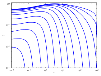
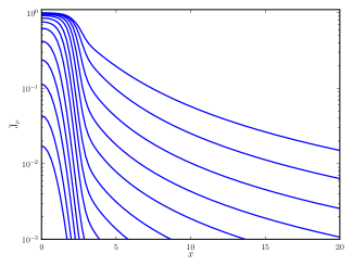
Figure 1: Plot of the static, two-level source function, $\bar{\rm J}$ for the $j=0\rightarrow 2$ transition as a function of $\tau$ (top panel); and the angle averaged intensity ${\rm J}_{\nu}$ as a function of frequency in Doppler widths, $x$ (bottom panel). In the bottom plot, the results are shown at $\tau=0$. Calculations were performed for Model I (see §5.1). For both plots, each curve represents a distinct time, increasing monotonically from bottom to top. The curves are all normalized to the maximum value of an independently calculated steady-state solution (see §§4.2–4.3). The figure may be compared with the righthand top and bottom panels of Fig. 1 in Kunasz (1983).

Figure 1 shows the results of our calculations, which can be compared with the righthand top and bottom panels of Fig. 1 in Kunasz (1983). The top panel shows the two-level source function for the diffuse component, $\bar{\rm J}=(4\pi)^{-1}\int_{4\pi}d\Omega\int d\nu\varphi_{\nu}I_{\nu}^{\rm diff}$, as a function of reference depth, $\tau$, at several times. The bottom panel shows the angle-averaged intensity, ${\rm J}_{\nu}\equiv(4\pi)^{-1}\int_{4\pi}d\Omega I_{\nu}^{\rm diff}$, at $\tau=0$, as a function of $x$, for several times. The curves are all normalized to the maximum value of an independently calculated steady-state solution (see §§4.2–4.3). The different curves correspond to monotonically increasing values of the time from bottom to top in each panel. These times represent the closest values on our grid to those listed in Table 1 of Kunasz (1983). To the extent we were able to compare, our results are in excellent agreement with the earlier work, reproducing the main features and trends, and showing only slight quantitative disagreement in one of the plots. Though we show a comparison to only two figures for brevity, we are able to reproduce all of the essential results of Kunasz (1983).

The main features of Figure 1 are propagation of the external radiation through the medium with increasing time in the top panel, and the approach of the curves toward an independently calculated steady state solution in both panels as $t/T_{\rm ref}$ increases beyond the light crossing time $T_{\rm LC}$.

Using the same model for the external source, we performed a similar calculation using the three-level atomic model described in §2, and a Voigt line profile (Model II). In this case, the medium is no longer approximately static, leading to a non-negligible population in the first excited state, $j=1$ (see §5.2). This leads to a difference in the source functions for the $j=0\rightarrow 2$ and $j=1\rightarrow 2$ transitions compared to the two-level case, altering the diffuse radiation field in the medium.

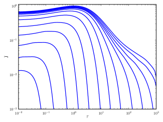
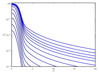
Figure 2: Same as Figure 1, except for the three level atomic model (Model II of §5.1). The quantities shown were computed using the radiation field within $x\leq 20$ of line centre for the $j=0\rightarrow 2$ transition.

Figure 2 is identical to Figure 1, except that it shows results for the three-level model, using the radiation field within $x\leq 20$ of line centre for the $j=0\rightarrow 2$ transition. With this atomic model, the radiation field exhibits a stronger depression at large reference depths, as well as a slightly softer line profile at $\tau=0$. This is caused by the fact that, in contrast to the static two-level model, not every excitation to $j=2$ results in a decay to $j=0$; a fraction of de-excitations are to the $j=1$ level, determined by the values of the populations and the Einstein coefficients for each transition. An important feature of Figures 1 and 2 is that the magnitude of the angle-averaged diffuse field becomes a significant fraction of the external $J_{\nu}$ only after an interval $\gtrsim T_{\rm ref}$. This is expected, as $T_{\rm ref}$ represents the characteristic time interval between successive radiative interactions. This point is important for judging whether a given astrophysical system will exhibit time coupled effects in radiative transfer (see §6).

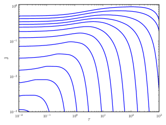
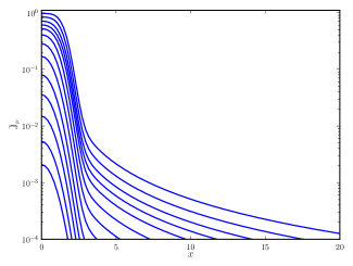
Figure 3: Same as Figure 2, except results are shown for the radiation field within $x\leq 20$ of line centre for the $j=1\rightarrow 2$ transition.

Figure 3 is identical to Figure 2, except that it shows results at frequencies $x\leq 20$, measured from line centre of the $j=1\rightarrow 2$ transition. The results are similar to those described above, except that the radiation experiences relatively smaller extinction at large reference depth. This is due to the fact that the effective optical depth for the excited state transition is much smaller than that for the ground state resonant transition (see §5.2). As in Model I, the results for Model II converge to an independently calculated steady-state as $t$ becomes larger than $T_{\rm LC}$.

§IIId and §IV of Kunasz (1983) present a detailed analysis of the method of lines solution to the radiative transfer equation in a two-level, static medium, analysing both its stability and effectiveness for various test problems. We have come to similar conclusions regarding our solution for the three-level, time-dependent medium. Briefly, we note that for $\bar{\theta}\lesssim 0.6$, unphysical oscillations can be introduced into the solution (though this can be mitigated somewhat by reducing the time and space grid spacings). Also, as the time and space grid resolution is increased, the results approach a final, converged solution with respect to the grid spacing. As in previous works, we find that distinct spacing in the time and space grids leads to an approximate representation of the propagation of the leading front of the external radiation. As long as the time interval for integration is not too large compared to $\tau_{\rm max}T_{\rm ref}$, we can use a linear time grid of sufficiently small spacing to provide an adequate sampling of the variation of the radiation field at all reference depths.

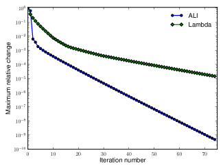
Figure 4: Maximum relative change in the level populations as a function of iteration number for the ALI and Lambda iteration methods applied to Model II of §5.1.

Apart from the solution to the RTE itself, the central concern of our method is the convergence of the atomic level populations. Figure 4 shows the maximum relative change in the populations of levels $n_{0}$, $n_{1}$, and $n_{2}$, for all time and space grid points, at each iteration during the solution. The curves marked by diamond and circle shaped symbols show the relative population change when Lambda and ALI iteration is used, respectively. As expected, the ALI method has a steeper slope and converges more quickly for a given number of iterations than the Lambda method. The results shown in Figure 4 are fairly typical for the models presented in this paper; in fact, the convergence properties are often better for Models III–VI than for Model II. For practical implementation of our methods with more complicated atomic models, it will likely prove useful to supplement the ALI iteration with additional acceleration methods, for example, Ng’s method or the generalized minimum residual method (for a detailed discussion of acceleration techniques, see, e.g., Auer, 1991).

As we increased the spatial grid resolution, the number of required iterations to reach a given relative accuracy also increased; this is a well known phenomenon (see Olson et al., 1986). However, this was typically not true of the time grid resolution. As discussed in §4.4, the initial guess for the solution at each time step is the converged solution for the previous time step. The finer the time grid resolution, the more similar the solution is in consecutive steps. Thus, increasing the time grid resolution tends to reduce the number of iterations per step. Since a reduction in spatial grid spacing is typically accompanied by a reduction in time grid spacing, the two effects will tend to counteract one another, and the increase in spatial grid resolution will not adversely affect the required number of iterations as much as expected. This is an unexpected benefit from applying the ALI method to the time-dependent problem.

5.2 Canonical Transient Pulse (Model III)

A class of external sources of immediate interest for this paper are those exhibiting transient behaviour, in which the amplitude of the transient pulse, $A$, is much greater than the background intensity $I_{\rm B}$. We constructed a canonical model for transient sources, using equation (6), with parameter values $I_{\rm B}/I_{\rm o}=10^{-5}$, $A/I_{\rm o}=0.1$, $t_{0}/T_{\rm ref}=5\times 10^{2}$, and $\sigma=0.5$ (Model III). We assumed that the external source was collimated, according to the prescription of §4.1. In our calculations, we used grid resolutions of $K=280$, $D=280$, $N=20$, and $M=40$. The time grid was spaced linearly over the interval $[0,4T_{\rm LC}]$.

For our atomic model, we used the three-level system described in §2, with a common, Doppler line profile for all three transitions. The initial condition for the radiation field and atomic level populations was the steady-state solution at $t/T_{\rm ref}=0$ (see §§4.2–4.3).

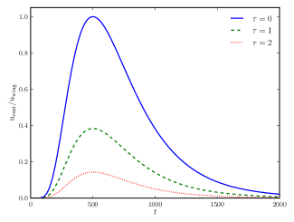
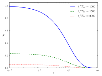
Figure 5: Radiation field for the $j=0\rightarrow 2$ transition with $\mu=1$. The top panel shows the line decrement $u_{\rm cent}/u_{\rm wing}$ (see the definition in §5.2) for several values of the reference depth. The bottom panel shows the radiation variable $u_{\nu}$ as a function of reference depth at several times. In the bottom panel, the variable $u_{\nu}$ is normalized to its maximum value in the $t/T_{\rm ref}=1000$ curve. The time is measured in units of $T_{\rm ref}$. All calculations have been performed for the canonical Model III of §5.2.

We define the decrement in the radiation field associated with a given transition as the value of $u_{\nu}$ at line centre ($x=0$) divided by the value in the line wing ($x=4$). The decrement is denoted $u_{\rm cent}/u_{\rm wing}$. Figure 5 shows the results of our calculation for the the $j=0\rightarrow 2$ transition, with direction $\mu=1$. The top panel shows the line decrement as a function of $t$ at several reference depths, $\tau=0,1,2$. The time $t$ is measured in units of $T_{\rm ref}$. Larger depths are not plotted, as the radiation field is negligible due to large extinction at $\tau\gg 1$. The peak intensity occurs at $t/T_{\rm ref}\approx 500$, when the external radiation has its maximum value. At $\tau=0$, there is little radiation re-emitted in the $\theta>0$ direction, implying that $u_{\nu}\approx I_{\nu}^{-}/2\approx I_{\nu}^{\rm ext}/2$. The bottom panel of Figure 5 shows $u_{\nu}$ as a function of $\tau$ for several times: $t/T_{\rm ref}=1000,1500,2000$. These times correspond to $T_{\rm LC},1.5T_{\rm LC}$, and $2T_{\rm LC}$, respectively. The curves in the bottom panel are normalized to the maximum value of $u_{\nu}$ at $t/T_{\rm ref}=1000$.

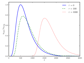
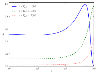
Figure 6: Same as Figure 5, except results are shown for the $j=1\rightarrow 2$ transition at reference optical depths $\tau=0,100,1000$.

Figure 6 is similar to Figure 5, except that it shows results for the $j=1\rightarrow 2$ transition. The radiation field is non-zero at larger reference depths than in the transition $j=0\rightarrow 2$ because the effective optical depth for the $j=1\rightarrow 2$ transition is smaller. This is due to the reduced population of the excited state relative to the ground state, as well as the smaller Einstein absorption coefficient for the $j=1\rightarrow 2$ transition compared to the resonant transition. It should be noted that most of the extinction in this transition occurs for $\tau<100$. The radiation field at frequencies near the resonant transition, which is necessary for the excitation event $j\rightarrow 2\rightarrow 1$, is largely damped at $\tau=100$. Thus, there are few excitation events to $j=1$ at $\tau>100$, and therefore little difference in the extinction from the $j=1\rightarrow 2$ transition at $\tau=100$ versus $\tau=1000$.

The smaller extinction is also evident in the bottom panel of Figure 6, in which the crossing of the spatial radiation profile through the $\tau=\tau_{\rm max}$ boundary is evident as time increases. As expected, the maximum of the radiation pulse is shifted to later times at larger reference depths. This is due to the fact that the light crossing time is of order the variability timescale for the radiation source. This feature is absent from Figure 5 because the reference depths plotted are small compared to $T_{\rm LC}/T_{\rm ref}$.

The results for the radiation field at frequencies around line centre of the $j=0\rightarrow 1$ transition are similar to those shown in Figure 6, except for the absence of significant extinction, due to the small value of the Einstein absorption coefficient for this transition.

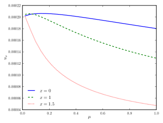
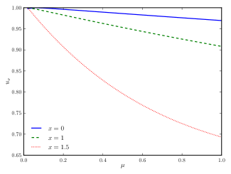
Figure 7: Radiation variable $u_{\nu}$ as a function of $\mu$ for several values of frequency in units of Doppler width, $x$. The top and bottom panels show results at $\tau=0$ and $\tau=\tau_{\rm max}$ for times $t/T_{\rm ref}=500$ and $t/T_{\rm ref}=500+\tau_{\rm max}$, respectively. All calculations were performed for the canonical Model III of §5.2.

Figure 7 shows the angular profile of the radiation at several frequencies around line centre of the $j=0\rightarrow 2$ transition. Results are plotted at $x=0,1,$ and $1.5$. The top panel shows the values of the $u_{\nu}$ radiation field variable at $\tau=0$ for $t/T_{\rm ref}=500\,T_{\rm ref}$, when the external source peaks at the inner boundary. The bottom panel shows the values of $u_{\nu}$ at $\tau=\tau_{\rm max}$ for $t/T_{\rm ref}=1500\,T_{\rm ref}$, when the peak of the external radiation passes through the outer boundary. We show the results for the diffuse field only; therefore, values at $\mu=1$ are excluded from the plots. All curves are normalized to the maximum value of $u$ at each frequency $x$. The plots demonstrate that the radiation field remains highly collimated at the $\tau=0$ boundary but is largely isotropic at $\tau_{\rm max}$ except at $x>1$. This result makes sense: because the optical depth in the $j=0\rightarrow 2$ transition is large, photons that reach $\tau=\tau_{\rm max}$ have experienced many atomic interactions and have been redistributed isotropically in angle. By contrast, the angular distribution of photons at the $\tau=0$ boundary is largely set by the external radiation; only backscattered photons from nearby layers of the slab are redistributed in angle at $\tau=0$. The medium therefore transitions from highly collimated to largely isotropic with intermediate results at $\tau\gtrsim 1$.

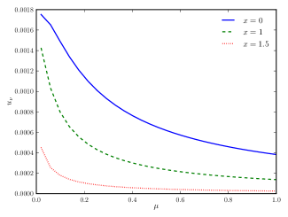
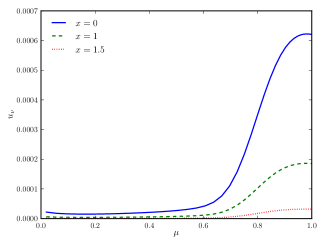
Figure 8: Same as Figure 7, except for frequencies around the $j=1\rightarrow 2$ transition.

Figure 8 is the same as Figure 7 except that it shows results for frequencies around the $j=1\rightarrow 2$ transition. In both cases, the radiation with $\theta>0$ is a small fraction of $u_{\nu}$ at $\tau=0$. However, for the $j=1\rightarrow 2$ transition, the radiation field remains highly anisotropic even at $\tau=\tau_{\rm max}$. This is due to the fact that this transition has a small effective optical depth (see below). Therefore, a small fraction of photons reaching $\tau=\tau_{\rm max}$ have been absorbed and redistributed into angles $\mu\neq 1$. The radiation in the $j=0\rightarrow 1$ transition exhibits a nearly identical angular profile to the $j=1\rightarrow 2$ transition.

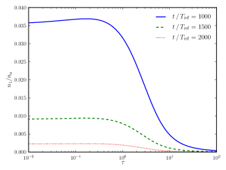
Figure 9: Level population of the first excited state, $n_{1}/n_{\rm o}$ as a function of time in units of $T_{\rm ref}$, for several reference depths (top panel); and as a function of reference depth for several times (bottom panel). All calculations have been performed for the canonical Model III of §5.2.

Figure 9 shows the level population of the excited state, $n_{1}/n_{\rm o}$ as a function of time in units of $T_{\rm ref}$. Since the upper level, $j=2$, remains negligibly populated throughout the calculation, the ground state population is $n_{0}/n_{\rm o}\approx 1-n_{1}/n_{\rm o}$. The top panel shows $n_{1}/n_{\rm o}$ as a function of $t/T_{\rm ref}$ at several reference depths, $\tau=0,2,5$. The bottom panel shows $n_{1}/n_{\rm o}$ as a function of $\tau$ for several times, $t=T_{\rm lc},1.5T_{\rm lc},2T_{\rm lc}$. The population of the excited state peaks at $t/T_{\rm ref}\approx 500$, which is when the radiation field close to the $\tau=0$ boundary has its maximum. The $j=0\rightarrow 2$ transition, followed by a spontaneous decay $j=2\rightarrow 1$, is the primary mechanism for populating the $j=1$ level. Since the radiation field in the $j=0\rightarrow 2$ transition rapidly decreases at line centre for $\tau\gg 1$, most of the excitation events occur at $\tau\lesssim 1$. This explains why the population of the excited state peaks with the external radiation in the top panel: the light travel time to the layers in which significant excitation occurs is relatively small compared to the timescales over which variation occurs. It is interesting to note that, as seen in the $t=T_{\rm LC}$ curve in the bottom panel of Figure 9, the population $n_{1}$ actually has its maximum value at $\tau\approx 0.2$. This is due to the fact that the external radiation has not yet been significantly extinguished, while the diffuse field is generated by absorption and re-emission into non-zero angles. The combination of these effects causes the radiation field in the $j=0\rightarrow 2$ transition to peak at $\tau>0$, leading to a maximum in the $n_{1}$ population at the same point.

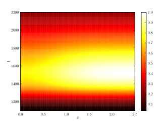
Figure 10: Time development of the $u_{\nu}$ line profile as a function of $x$. Results are shown for $\tau=\tau_{\rm max}$ and $\mu=1$. The time is given in units of $t/T_{\rm ref}$, while the intensity scale is normalized to the maximum value of the radiation field, which occurs at $t/T_{\rm ref}\approx 1500$ for $x=4$. The calculations were performed for the canonical Model III of §5.2.

Figure 10 shows the time development of the $j=1\rightarrow 2$, $u_{\nu}$ line profile as a function of $x$, at $\tau=\tau_{\rm max}$ with $\mu=1$. The intensity scale is normalized to the maximum value of the radiation field, which occurs at $t/T_{\rm ref}\approx 1500$ for $x=4$. At line center ($x=0$), the field decreases to its minimum intensity approximately when photons from the peak emission of the external source cross the medium; as expected, this is when the field in the line wing ($x=4$) achieves its maximum intensity. When the medium contains a significant fraction of atoms in the $j=1$ state, absorption at line center decreases the intensity of the radiation field at earlier times than for frequencies $x>0$. At $t/T_{\rm ref}>1800$, when the atoms have depopulated to the ground state, the time variation of photons at all frequencies is once again the same.

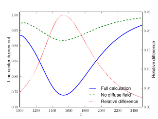
Figure 11: Line decrement at $\mu=1$, $\tau=\tau_{\rm max}$, defined as the radiation variable $u_{\nu}$ at line centre divided by its value in the line wing ($x=4$), $u_{\rm cent}/u_{\rm wing}$. The decrement is shown as a function of time in units of $T_{\rm ref}$. The solid and dashed curves show results from the full calculation and collimated approximation, respectively. The dotted curve shows the relative difference between the full calculation and approximation. All calculations have been performed for the canonical Model III of §5.2.

Figure 11 shows $u_{\rm cent}/u_{\rm wing}$ for the $j=1\rightarrow 2$ transition, at $\tau=\tau_{\rm max}$ and $\mu=1$, as a function of time (solid curve). The decrement can be used to define an effective optical depth,

$$\tau_{\rm eff}\equiv-\log(u_{\rm cent}/u_{\rm wing});$$ (68)

for the canonical Model III, $\tau_{\rm eff}\approx 0.3$. As expected, the peak effective optical depth in the $j=1\rightarrow 2$ transition occurs at time $t/T_{\rm ref}\approx\tau_{\rm max}+500$, which corresponds to the time at which photons from the peak of the external source cross the medium. These photons experience large extinction at line centre due to excitation of the atoms into the $j=1$ level.

Several previous works in the literature have used simplified treatments of radiative transfer to infer the state of atomic populations in absorbing material around GRBs from the effective optical depth in absorption lines of afterglow specra (see §6). These works neglected the diffuse field in their solution to the radiative transfer equation; we refer to this solution as the ‘collimated approximation’ (see, e.g., Vreeswijk et al., 2007; D’Elia et al., 2009; Robinson et al., 2010). In this case, the external radiation is propagated through the slab, but angularly redistributed photons are neglected in determining the values of the level populations. In this approximation, the calculation becomes much simpler, and the convergence of the level populations is almost immediate. The result is shown by the dashed curve in Figure 11. Clearly, significant errors are introduced into the calculation of the decrement when the diffuse component of the radiation field is neglected. This is due to the fact that neglecting the diffuse field implies a lower excitation rate of atoms from the ground state to $j=1$. If $T_{\rm VR}$ is of order $T_{\rm ref}$, then the line centre extinction for photons propagating through the medium will be increased when the diffuse field is taken into account, resulting in a larger decrement.

5.3 Variation of Model Parameters (Models IV–VI)

In this section, we explore the effects of changing the atomic physics; the transient amplitude, $A$; and the value of the background radiation, $I_{\rm B}$.

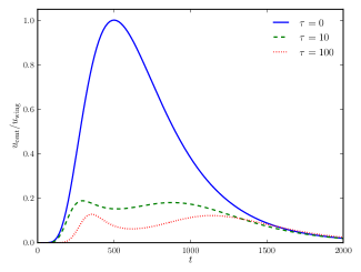
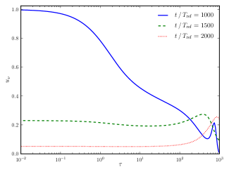
Figure 12: Same as Figure 6, except that results are shown for Model IV of §5.3.

We performed a similar calculation to that described in Model III, except that we multiplied the Einstein coefficients for the $j=1\rightarrow 2$ transition by a factor of ten (Model IV). Figure 12 is identical to Figure 6 except that it shows results for Model IV. In addition, the results in the top panel were computed for $\tau=0,10,100$. The figure indicates that the effective optical depth for the $j=1\rightarrow 2$ transition is much larger for Model IV than for Model III. An interesting feature in the top panel of Figure 12 is the slight decrease in the intensity around $t/T_{\rm ref}=\tau+500$, where the radiation field peaks in Figure 6. The new feature occurs because of the increase in the population of the $j=1$ level, resulting in larger extinction. Most photons with frequencies near line centre of the $j=1\rightarrow 2$ transition that pass through spatial point $\tau\approx 500$ at time $t/T_{\rm ref}=\tau+500$ originated in the peak of the external radiation. However, the intensity exhibits an overall decrease due to the enhanced extinction. Such a feature was absent from Figure 6 because the total extinction was too small to compensate for the increase in intensity from the external boundary. The same phenomenon is responsible for the dip in intensity around $\tau\approx 500$ in the solid curve ($t=T_{\rm LC}$) of the bottom panel.

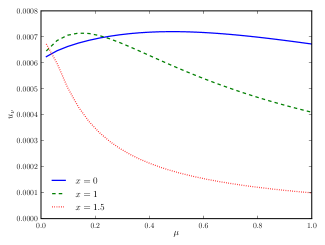
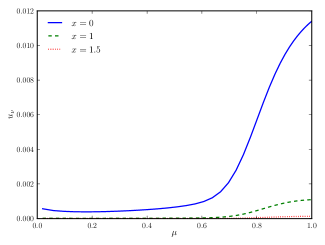
Figure 13: Same as Figure 8, except that results are shown for Model IV of §5.3.

Figure 13 shows the angular distribution of radiation for Model IV. The results are similar to those in Figure 8 for Model III, with the radiation field exhibiting increased isotropy at $\tau=\tau_{\rm max}$, due to increased angular redistribution reflected in the larger value of the effective optical depth.

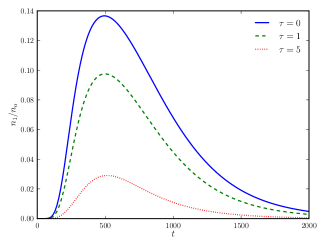
Figure 14: Same as the top panel of Figure 14, except that results are shown for Model IV of §5.3.

Figure 14 is identical to the top panel of Figure 9, except that it shows $n_{1}/n_{\rm o}$ as a function of time at $\tau=0,1,5$. At small reference depths, we see an increase in the maximum population of level $j=1$; this is due to the increase in the spontaneous emission coefficient for the $j=2\rightarrow 1$ transition.

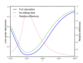
Figure 15: Same as Figure 11, except that results are shown for Model IV of §5.3.

Figure 15 shows the decrement in the $j=1\rightarrow 2$ transition as a function of time in units of $T_{\rm ref}$. The plot exhibits the same overall features as Figure 11, except that the maximum effective optical depth at $t/T_{\rm ref}\approx\tau_{\rm max}+500$ is $\tau_{\rm eff}\approx 3$. The larger Einstein coefficients for the $j=1\rightarrow 2$ transition cause increased extinction per excitation event. Thus, while both the full calculation and the collimated approximation exhibit enhanced extinction, there is a larger relative error associated with employing the latter (up to 100%) compared to Model III. This is due to the fact that there are fewer excitations to the $j=1$ level in the collimated approximation due to the neglect of the diffuse field, and this error is amplified in the extinction by the change in atomic physics for Model IV.

We performed another calculation using the same parameters and Einstein coefficients as in Model III, except for an increase in the amplitude of the transient component of equation (6) to $A=1$ (Model V).

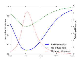
Figure 16: Same as Figure 11, except that results are shown for Model V of §5.3.

Figure 16 is identical to Figure 15, except that it shows results for Model V. The maximum effective optical depth in the $j=1\rightarrow 2$ transition is $\tau_{\rm eff}\approx 3$. However, the relative error introduced into the calculation by neglecting the diffuse field has increased by a factor of six. This is due to the increase in the maximum amplitude of the external radiation. In Model IV, the increased extinction relative to Model III resulted from the stronger $j=1\rightarrow 2$ transition in the atomic model, which affected both the full calculation and the collimated approximation. In Model V, the increased extinction relative to Model III is due to enhanced excitation to the $j=1$ level; this affects the full calculation and the collimated approximation differently. In the former, inclusion of the diffuse field fully incorporates the effect of increasing the external radiation amplitude. In the latter, a significant fraction of the amplitude increase is neglected, leading to a smaller effective optical depth for the collimated approximation relative to Model IV.

We explore a final case in which the background radiation is a significant fraction of the transient amplitude (Model VI). For this case, we change the parameters of the canonical Model III to $I_{\rm B}/I_{\rm o}=0.1$ and $A/I_{\rm o}=1$.

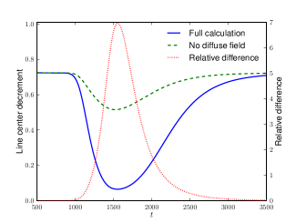
Figure 17: Same as Figure 11, except that results are shown for Model VI of §5.3.

For the most part, the results for Model VI are similar to those for Model V. This is not unexpected as the maximum amplitude of the transient component of the external source is the same in both cases. One major difference is that the system begins and relaxes to an equilibrium state in which the diffuse field and excited $j=1$ level population are non-zero. At reference depth $\tau=0$ for times $t/T_{\rm ref}=0$ and $t/T_{\rm ref}>10^{3}$, the excited state populations are $n_{1}/n_{\rm o}\approx 0.08$ (note that this is approximately equal to the maximum population at $\tau=0$ for Model III). Figure 17 shows the line decrement results for Model VI. At $t<T_{\rm LC}$, the line decrement is equal to its equilibrium value, $u_{\rm cent}/u_{\rm wing}\approx 0.75$. After a light crossing time, it decreases until the effective optical depth is $\tau_{\rm eff}\approx 3$, after which it relaxes back to its equilibrium value.

The collimated approximation was altered slightly for the calculations of Model VI. In this case, the steady-state diffuse field was determined at $t/T_{\rm ref}=0$ and held fixed during the calculation; only the collimated radiation was allowed to vary dynamically. As in Model V, the relative error introduced by neglecting changes in the diffuse field is significant, greater than $600\%$ at maximum.

6 Discussion

We have developed a general formalism for the numerical solution of the TDRTE and atomic rate equations using ALI. We applied our method to a three-level atomic model that included allowed transitions between the ground and first excited states to a common upper level, as well as a forbidden transition between the two former states. Our calculations exhibit convergence of the iterative ALI method and, when augmented with additional acceleration techniques, can be used in efficient calculations of line transfer with realistic atomic models. Our results show time coupled effects in the evolution of the atomic level populations, radiation field, and emergent spectra. We have compared our solution to an approximate treatment in which photons that are redistributed in angle are neglected (i.e., the diffuse field is ignored), and showed that this approximation results in errors of $20-600\%$ in the effective optical depth for the $j=1\rightarrow 2$ transition. This error increases with the magnitude of $\tau_{\rm eff}$. The effect occurs because the diffuse field photons affect the level populations and extinction coefficient for the excited state transition. If the time variability of the source falls in the intermediate regime (see §1), then photons passing through the medium along the line of sight experience increased extinction when the diffuse radiation field is included in the calculation.

These conclusions are relevant for timescales obeying the relations $T_{\rm VR}\gtrsim T_{\rm ref}$ and $T_{\rm VR}\lesssim T_{\rm LC}$. Assuming a Doppler line profile in complete redistribution, we can write the ratio $T_{\rm VR}/T_{\rm ref}$ as

$$\begin{split}\frac{T_{\rm VR}}{T_{\rm ref}}&=0.893\left(\frac{T_{\rm VR}}{10^{3}\text{ s}}\right)\left(\frac{10^{-5}}{b/c}\right)\\ &\times\left(\frac{B_{02}}{10^{9}\text{ cm}^{2}\text{ s}^{-1}\text{ erg}^{-1}}\right)\left(\frac{n_{\rm o}}{\text{cm}^{-3}}\right),\end{split}$$ (69)

and the maximum optical depth as

$$\begin{split}\tau_{\rm max}&=2.98\left(\frac{W}{10^{14}\text{cm}}\right)\left(\frac{10^{-5}}{b/c}\right)\\ &\times\left(\frac{B_{02}}{10^{9}\text{ cm}^{2}\text{ s}^{-1}\text{ erg}^{-1}}\right)\left(\frac{n_{\rm o}}{\text{cm}^{-3}}\right).\end{split}$$ (70)

If the timescales characterizing the external radiation source and medium satisfy the intermediate regime inequalities, then radiation transfer in the astrophysical system should be treated using the ALI methods developed in this paper. If, however, $T_{\rm VR}\ll T_{\rm ref}$, then the collimated approximation can be used without loss of accuracy. This is due to the fact that the diffuse radiation field is generated on timescales $\gtrsim T_{\rm ref}$, and if the transient pulse propagates through the medium on smaller timescales, then the level populations will not be altered by the diffuse field in time to affect extinction of the external photons. Conversely, if $T_{\rm VR}\gg T_{\rm LC}$, then the radiation field is determined by the steady-state RTE.

Using the scaling of the quantities in equations (69) and (70), we can draw conclusions about what kind of astrophysical systems require the full TDRTE solution presented in this paper. In all cases, we assume that the characteristic transition has an Einstein coefficient $B_{02}\sim 10^{9}$ cm² s^-1 erg^-1.

In absorbing systems composed of metal ions with $n_{\rm o}\sim 10^{-5}$ cm^-3, if the width of the medium is $W\gtrsim 1$ pc (corresponding to a minimum $\tau_{\rm max}\sim 1$), then the time variability of the external source must be $T_{\rm VR}\gtrsim 10^{8}$ s for the full ALI solution to apply. In contrast, for absorbing systems at a higher density, $n_{\rm o}\sim 1$ cm^-3, the full ALI solution applies when $T_{\rm VR}\sim 10^{3}$ s and $W\gtrsim 3\times 10^{13}$ cm.

Time variability is common in astrophysical sources. Notable examples of highly transient emitters are GRBs, which emit prompt $\gamma$-ray emission at early times, followed by longer wavelength afterglow radiation in the X-ray, UV and optical bands. The afterglow emission occurs on timescales that range from minutes to days. A large number of studies have examined the time dependence of afterglow absorption spectra due to photoionization of the medium; this variability occurs on timescales comparable to the observation time (Perna & Loeb, 1998; Böttcher et al., 1999; Perna & Lazzati, 2002; Lazzati & Perna, 2002; Mirabal et al., 2002; Robinson et al., 2010). Observations of time-dependent absorption have been reported for a number of GRBs (Thöne et al., 2011; Vreeswijk et al., 2012; De Cia et al., 2012). In a few cases, excitation of fine line transitions of Fe II were observed in the absence of appreciable photoionization (Vreeswijk et al., 2007; D’Elia et al., 2009). So far, none of the time-dependent radiative transfer calculations developed specifically for GRBs has included source terms for the diffuse field. Previous work emphasized the modelling of time-dependent absorption effects due to photoionization, rather than the details of line transfer.

Consider the results of our analysis for a GRB variability timescale of $T_{\rm LC}\sim 10^{3}$ s, and typical interstellar medium hydrogen density of $n_{\rm H}\sim 1$ cm^-3. For metal ions with $n_{\rm o}\sim 10^{-5}$ cm^-3, the condition $T_{\rm VR}\ll T_{\rm ref}$ is satisfied, and the collimated approximation is appropriate. However, for hydrogen, $T_{\rm VR}\sim T_{\rm ref}$, and the diffuse field can affect line transfer through the absorber, coupling to the photoionization state. Thus, more detailed studies, using the methods described in our paper, should be performed when interpreting observations of afterglow line variability. In addition, if the GRB occurs in a molecular cloud, with densities as high as $\sim 10^{5}$ cm^-3, then a full solution to the time-dependent line transfer problem may be needed even for metal lines.

AGNs form another important class of time variable sources. Typical AGN soft X-ray variability timescales range from $\sim 1$ ksec in nearby, small black hole mass Seyfert galaxies, to $\sim 100$ ksec in distant, massive quasars (Fiore et al., 1998). The central source is surrounded by a cloud of absorbers with hydrogen densities as high as $\sim 10^{7}-10^{8}$ cm, located at distances of $\sim 10^{13}-10^{14}$ cm (Baldwin et al., 1995; Krongold et al., 2007). If the source variability is about $1$ ksec for an absorber with density $n_{\rm o}\sim 10^{3}$ cm^-3 (in metal lines), then $T_{\rm VR}\sim 10^{3}\,T_{\rm ref}$. In this case, the full time-dependent formulation of line transfer is needed when $\tau_{\rm max}\gtrsim 10^{3}$, implying an absorber width of $W\gtrsim 3\times 10^{13}$ cm. If the source variability timescale is longer, with $T_{\rm VR}\sim 100$ ksec, then the full solution is required when $\tau_{\rm max}\gtrsim 10^{5}$, implying an absorber width of $W\gtrsim 3\times 10^{15}$ cm.

The examples above illustrate that, for any time variable source, there is a range of absorber properties for which line transfer must be treated by the ALI method.

In Appendix A, we further generalize our formalism to include a broad class of Runge-Kutta methods for the time integrations employed in §4. These techniques will enable future calculations that monitor the error in the time grid discretization, or implement an adaptive time step algorithm. Such improvements can improve the stability of the radiation field integration, reduce artificial oscillations in the solution, and allow more efficient calculations for realistic atomic models.

Appendix A Runge-Kutta Methods

In this Appendix, we outline how the iterative scheme of §4.4 can be implemented with implicit Runge-Kutta methods (see, e.g., §II.7 of Hairer et al., 1991). For simplicity, we neglect collisions in the rate equations and background contributions to the emissivity. Including these terms requires a straightforward generalization of the work below.

Applying the method of lines to the simultaneous system of equations yields (c.f., §4.2):

$$f_{j,d} =\sum_{l}\bigl{(}R_{lj,d}n_{l,d}-R_{jl,d}n_{j,d}\bigr{)},$$ (71)

$$\begin{split}f_{u,di}&=c\chi_{di}\Bigl{[}\left(v_{d+1/2,i}-v_{d-1/2,i}\right)/\Delta\tau_{di}\\ &\qquad\qquad-u_{di}+S_{di}\Bigr{]},\end{split}$$ (72)

$$\begin{split}f_{v,d+1/2,i}&=c\chi_{d+1/2,i}\Bigl{[}\left(u_{d+1,i}-u_{di}\right)/\Delta\tau_{di}^{+}\\ &\qquad\qquad\qquad-v_{d+1/2,i}\Bigr{]}.\end{split}$$ (73)

Note that we used a second order spatial discretization above, though more complicated methods are possible. Higher order methods will lead to a more complicated spatial structure for the linear systems of equations (see below).

The Runge-Kutta solution for equation (71) can be written

$$n_{j,kd}=n_{j,k-1,d}\\ +\Delta t_{k}\sum_{p=0}^{P-1}b_{p}f_{j,d}\left(t_{k-1}+c_{p}\Delta t_{k},n_{j,kd}^{p}\right),$$ (74)

with

$$n_{j,kd}^{p}=n_{j,k-1,d}+\Delta t_{k}\sum_{p^{\prime}=0}^{P-1}a_{pp^{\prime}}f_{j,d}\Bigl{(}t_{k-1}\\ +c_{p}^{\prime}\Delta t_{k},n_{j,kd}^{p^{\prime}},n_{l,kd}^{p^{\prime}},\ldots\Bigr{)},$$ (75)

where $P$ is the number of stages, and $c_{p}$, $a_{pp^{\prime}},b_{p}$ are the coefficients for the Runge-Kutta method. The notation $n_{j,kd}^{p^{\prime}},n_{l,kd}^{p^{\prime}},\dots$ indicates that the $p^{\prime\rm th}$ stage quantities for each level are substituted in the expression for $f_{j,d}$. In equations (74) and (75), $f_{j,d}$ contains a dependence on $u_{d}$ through the quantities $R_{ld,d}$ defined in §4.3.

We can use the Runge-Kutta solution to equation (73) to simplify the dependence on $v$ in (72):

$$v_{k,d+1/2,i}^{p}=v_{k-1,d+1/2,i}+\Delta t_{k}\sum_{p^{\prime}=0}^{P-1}a_{pp^{\prime}}c\chi_{k,d+1/2,i}^{p^{\prime}}\\ \times\left[\left(u_{k,d+1,i}^{p^{\prime}}-u_{kdi}^{p^{\prime}}\right)/\Delta\tau_{kdi}^{p^{\prime}+}-v_{k,d+1/2,i}^{p^{\prime}}\right],$$ (76)

where the quantities $\Delta\tau_{kdi}^{p^{\prime}+}$ and $\chi_{k,d+1/2,i}^{p^{\prime}}$ are evaluated at $t_{k-1}+c_{p^{\prime}}\Delta t_{k}$ using the values $n_{j,kd}^{p^{\prime}}$. This is a linear system of dimension $P$ in the quantities $v_{k,d+1/2,i}^{p}$. If we define the column vector

$${\bf v}_{k,d+1/2,i}=\left(v_{k,d+1/2,i}^{p=0},\ldots v_{k,d+1/2,i}^{p=P-1}\right)^{T},$$ (77)

we can write the system as

$$\mathbf{L}_{k,d+1/2,i}\cdot{\bf v}_{k,d+1/2,i}=\\ {\bf M}_{k,d+1/2,i}\cdot\left({\bf u}_{k,d+1,i}-{\bf u}_{kdi}\right)+{\bf v}_{k-1,d+1/2,i},$$ (78)

where the elements of the $P\times P$ matrices ${\bf L}_{k,d+1/2,i}$ and ${\bf M}_{k,d+1/2,i}$ are determined by equation (76). The elements of the vector ${\bf v}_{k-1,d+1/2,i}$ are all equal to $v_{k-1,d+1/2,i}$. The solution to equation (78) can be obtained in $\mathcal{O}(P^{3})$ operations for each triple of indices $(k,d+1/2,i)$. We write this solution as:

$${\bf v}_{k,d+1/2,i}=\boldsymbol{\mathcal{M}}_{k,d+1/2,i}\\ \cdot\left({\bf u}_{k,d+1,i}-{\bf u}_{kdi}\right)+\boldsymbol{\mathcal{N}}_{k,d+1/2,i}.$$ (79)

We can substitute equation (79) into the Runga-Kutta formula for $u$ to obtain a formal solution for the diffuse radiation field. The Runge-Kutta solution for $u$ can be written:

$$u_{kdi}^{p}=u_{k-1,di}+\Delta t_{k}\sum_{p^{\prime}=0}^{P-1}a_{pp^{\prime}}c\chi_{kdi}^{p^{\prime}}\\ \times\Bigl{[}\left(v_{k,d+1/2,i}^{p^{\prime}}-v_{k,d-1/2,i}^{p^{\prime}}\right)/\Delta\tau_{kdi}^{p^{\prime}}\\ -u_{kdi}^{p^{\prime}}+S_{kdi}^{p^{\prime}}\Bigr{]}\Rightarrow$$ (80)

$${\bf L}_{kdi}\cdot{\bf u}_{kdi}={\bf M}_{kdi}\cdot\left({\bf v}_{k,d+1/2,i}-{\bf v}_{k,d-1/2,i}\right)\\ +{\bf N}_{kdi}\cdot{\bf S}_{kdi}+{\bf u}_{k-1,di},$$ (81)

where the matrices and vectors are defined analogously to those in the equation for the $v$ variable. If we substitute equation (79) into (81), we obtain a system of equations of the form:

$$\begin{split}-{\bf A}_{kdi}\cdot{\bf u}_{k,d-1,i}+\left({\bf L}_{kdi}+{\bf A}_{kdi}+{\bf C}_{kdi}\right)\cdot{\bf u}_{kdi}\\ -{\bf C}_{kdi}\cdot{\bf u}_{k,d+1,i}={\bf R}_{kdi}\cdot{\bf S}_{kdi}+{\bf B}_{kdi},\end{split}$$ (82)

where the vector ${\bf B}_{kdi}$ contains the dependences on the radiation variables at the previous time grid point, $k-1$. Equation (82) can be supplemented by boundary conditions connecting the points $d=0,1$ and $d=D-2,D-1$. These conditions can be derived as in §4.2: the method of lines is applied to first order, and the time integration proceeds as described above. Thus, we obtain a block tridiagonal linear system that can be solved in $\mathcal{O}\left(P^{3}D\right)$ operations for each $(k,i)$. We write the solution to equation (82) as

$$\tilde{\bf u}_{ki}=\tilde{\boldsymbol{\Lambda}}_{ki}\cdot\tilde{\bf S}_{ki}+\tilde{\bf B}_{ki},$$ (83)

where $\tilde{\boldsymbol{\Lambda}}_{ki}$ is a $D\times D$ block matrix with $P\times P$ matrices as elements, and $\tilde{\bf B}_{ki}$ is a $D\times 1$ block vector with $P\times 1$ vectors as elements.

To obtain a formal solution for the diffuse field, we augment our time grid with the points $\{t_{k-1}+c_{p}\Delta t_{k}\}$. The solution then consists of the values $u_{kdi}^{p=0},\ldots,u_{kdi}^{p=P-1}$, for $k=1,\ldots K-1$, where the quantities $u_{kdi}^{p=P-1}$ represent the solution on the original $K-1$ time grid points. Using the initial conditions, we can solve equation (83) successively for $k=1,\ldots K-1$. The structure of this formal solution in terms of the source functions $S_{kd}^{p}$ is quite complicated, coupling the various Runge-Kutta stages and spatial grid points. However, if we consider the ALI form of the formal solution,

$$u_{kdi}^{p}=\Lambda_{kdi}^{p*}\left(S_{kdi}^{p}-S_{kdi}^{p{\dagger}}\right)+u_{kdi}^{p{\dagger}},$$ (84)

we achieve a significant simplification. In equation (84), $\Lambda_{kdi}^{p*}$ denotes the diagonal elements of the $P\times P$ matrices that are in turn along the diagonal of the $D\times D$ block matrix $\tilde{\boldsymbol{\Lambda}}_{k}$. The source functions are evaluated with the level populations $n_{j,kd}^{p},n_{l,kd}^{p},\ldots,$ for the current and previous $({\dagger})$ iterations. The diagonal elements of $\tilde{\boldsymbol{\Lambda}}_{ki}$ can be obtained simultaneously with the formal solution, using the block matrix form of the equations in Appendix B of Rybicki & Hummer (1991). As in §4.4, we use the alternate form of the formal solution,

$$u_{kdi}^{p}=\Psi_{kdi}^{p*}\left(\eta_{kdi}^{p}-\eta_{kdi}^{p{\dagger}}\right)+u_{kdi}^{p{\dagger}}\\ =\Psi_{kdi}^{p*}\sum_{l,j}U_{lj,i}\left(n_{l,kd}^{p}-n_{l,kd}^{p{\dagger}}\right)+u_{kdi}^{p{\dagger}},$$ (85)

where $\Psi_{kdi}^{p*}=\Lambda_{kdi}^{p*}/\chi_{kdi}^{p{\dagger}}$.

We can substitute equation (85) into equation (75) and precondition the resulting non-linear expressions as described in §4.3 and §4.4. The ALI method then proceeds as follows: starting with the initial conditions, $u_{k=0,di}$, $n_{j,k=0,d}$, we solve for the formal solution at $k=1,\ldots,K-1$. At each $k$, we iterate over the populations $n_{j,kd}^{p}$ for all the atomic levels and Runge-Kutta stages, using the formal solution for $u_{kd}^{p{\dagger}}$, approximate matrix $\Lambda_{kd}^{p*}$, and ALI linear system. The method is completely analogous to the technique described in §4.4; indeed the equations in the main text are special cases of Runge-Kutta integrations with coefficients given by the Butcher tableaux 1 1 1 (Backward Euler) and 0 0 0 1 1/2 1/2 1/2 1/2 (Crank-Nicholson).

References

- Abdikamalov et al. (2012) Abdikamalov E., Burrows A., Ott C. D., Löffler F., O’Connor E., Dolence J. C., Schnetter E., 2012, ApJ, 755, 111
- Abel & Wandelt (2002) Abel T., Wandelt B. D., 2002, MNRAS, 330, L53
- Auer (1991) Auer L., 1991, in Crivellari L., Hubeny I., Hummer D. G., eds, NATO ASIC Proc. 341: Stellar Atmospheres - Beyond Classical Models. p. 9
- Auer et al. (1994) Auer L., Bendicho P. F., Trujillo Bueno J., 1994, A&A, 292, 599
- Baldwin et al. (1995) Baldwin J., Ferland G., Korista K., Verner D., 1995, ApJL, 455, L119
- Böttcher et al. (1999) Böttcher M., Dermer C. D., Crider A. W., Liang E. P., 1999, A&A, 343, 111
- Cannon (1973) Cannon C. J., 1973, ApJ, 185, 621
- Cannon (1985) Cannon C. J., 1985, The Transfer of Spectral Line Radiation. Cambridge: Cambridge University Press
- Davis et al. (2012) Davis S. W., Stone J. M., Jiang Y.-F., 2012, ApJS, 199, 9
- De Cia et al. (2012) De Cia A. et al., 2012, A&A, 545, A64
- D’Elia et al. (2009) D’Elia V., et al., 2009, ApJ, 694, 332
- Fiore et al. (1998) Fiore F., Laor A., Elvis M., Nicastro F., Giallongo E., 1998, ApJ, 503, 607
- Gnedin & Abel (2001) Gnedin N. Y., Abel T., 2001, NA, 6, 437
- Hairer et al. (1991) Hairer C. J., Nørsett S. P., Wanner G., 1991, Solving Ordinary Differential Equations I: Nonstiff Problems. New York: Springer-Verlag
- Harper (1994) Harper G. M., 1994, MNRAS, 268, 894
- Hauschildt (1993) Hauschildt P. H., 1993, JQSRT, 50, 301
- Hayek et al. (2010) Hayek W., Asplund M., Carlsson M., Trampedach R., Collet R., Gudiksen B. V., Hansteen V. H., Leenaarts J., 2010, A&A, 517, A49
- Hubeny (2003) Hubeny I., 2003, in Hubeny I., Mihalas D., Werner K., eds, Astronomical Society of the Pacific Conference Series Vol. 288, Stellar Atmosphere Modeling. p. 17
- Hubeny & Burrows (2007) Hubeny I., Burrows A., 2007, ApJ, 659, 1458
- Hubeny & Lanz (1995) Hubeny I., Lanz T., 1995, ApJ, 439, 875
- Juvela (1997) Juvela M., 1997, A&A, 322, 943
- Juvela & Padoan (2005) Juvela M., Padoan P., 2005, ApJ, 618, 744
- Krongold et al. (2007) Krongold Y., Nicastro F., Elvis M., Brickhouse N., Binette L., Mathur S., Jiménez-Bailón E., 2007, ApJ, 659, 1022
- Krumholz et al. (2012) Krumholz M. R., Klein R. I., McKee C. F., 2012, ApJ, 754, 71
- Kunasz (1983) Kunasz P. B., 1983, ApJ, 271, 321
- Kunasz & Olson (1988) Kunasz P. B., Olson G. L., 1988, JQSRT, 39, 1
- Kutepov et al. (1991) Kutepov A. A., Kunze D., Hummer D. G., Rybicki G. B., 1991, JQSRT, 46, 347
- Lazzati & Perna (2002) Lazzati D., Perna R., 2002, MNRAS, 330, 383
- Mihalas (1978) Mihalas D., 1978, Stellar Atmospheres. San Francisco: W. H. Freeman and Co.
- Mihalas & Klein (1982) Mihalas D., Klein R. I., 1982, Journal of Computational Physics, 46, 97
- Mirabal et al. (2002) Mirabal N. et al., 2002, ApJ, 578, 818
- Olson et al. (1986) Olson G. L., Auer L. H., Buchler J. R., 1986, JQSRT, 35, 431
- Perna & Lazzati (2002) Perna R., Lazzati D., 2002, ApJ, 580, 261
- Perna et al. (2003) Perna R., Lazzati D., Fiore F., 2003, ApJ, 585, 775
- Perna & Loeb (1998) Perna R., Loeb A., 1998, ApJ, 501, 467
- Robinson et al. (2010) Robinson P. B., Perna R., Lazzati D., van Marle A. J., 2010, MNRAS, 401, 88
- Rundle et al. (2010) Rundle D., Harries T. J., Acreman D. M., Bate M. R., 2010, MNRAS, 407, 986
- Rybicki (1972) Rybicki G. B., 1972, in Line Formation in the Presence of Magnetic Fields. p. 145
- Rybicki (1984) Rybicki G. B., 1984, Escape probability methods. pp 21–64
- Rybicki & Hummer (1991) Rybicki G. B., Hummer D. G., 1991, A&A, 245, 171
- Rybicki & Hummer (1992) Rybicki G. B., Hummer D. G., 1992, A&A, 262, 209
- Sellmaier et al. (1993) Sellmaier F., Puls J., Kudritzki R. P., Gabler A., Gabler R., Voels S. A., 1993, A&A, 273, 533
- Thöne et al. (2011) Thöne C. C. et al., 2011, MNRAS, 414, 479
- Uitenbroek (2001) Uitenbroek H., 2001, ApJ, 557, 389
- Vreeswijk et al. (2012) Vreeswijk P. M. et al., 2012, ArXiv e-prints
- Vreeswijk et al. (2007) Vreeswijk P. M. et al., 2007, A&A, 468, 83
- Whalen & Norman (2006) Whalen D., Norman M. L., 2006, ApJS, 162, 281