Accurate phase measurement with classical light

Abstract

In this paper we investigate whether it is in general possible to substitute maximally path-entangled states, namely NOON-states by classical light in a Doppleron-type resonant multiphoton detection processes by studying adaptive phase measurement with classical light. We show that multiphoton detection probability using classical light coincides with that of NOON-states and the multiphoton absorbtion rate is not hindered by the spatially unconstrained photons of the classical light in our scheme. We prove that the optimal phase variance with classical light can be achieved and scales the same as that using NOON-states.

I Introduction

Optical phase measurement is the basis of many scientific research areas, such as quantum metrology and quantum computing. The precision of optical phase measurement is bounded by the standard quantum limit (SQL) or shot noise limit (SNL) which scale as $1/\sqrt{N}$ in the number of $N$ independent resources. However, many authors Caves (1981); Yurke et al. (1986); Sanders et al. (1995) proposed the possibility to beat the SQL and reach the Heisenberg limit which scales as $1/N$ by using nonclassical states. One possibility to reach the Heisenberg limit is to use NOON states and combine them with an adaptive measurement scheme Berry et al. (2009)

NOON states are among the most highly-entangled states and they have the potential to enhance measurement precision Lee et al. (2002) not only in phase measurement Berry et al. (2009) but also in subwavelength lithography Boto et al. (2000) and atomic interferometry Wei et al. (2011).

However, due to the difficulty in generating NOON states with large photon number ($N>2$), alternative efforts have been made such as by the use of multiple passes of single photon Higgins et al. (2007) and dual Fock state Xiang et al. (2010). In the single photon scheme, the measurement time scales with $N$ which poses a problem for very fast measurement. In the dual Fock state scheme, a sub-SNL rather than Heisenberg limit is obtained. Moreover, number entangled states Boto et al. (2000) are criticized for being highly spatially unconstrained to be absorbed at a tiny spot Steuernagel (2004).

Recently, Hemmer et al. Hemmer et al. (2006) pointed out the quantum feature of path-number entanglement with NOON states can be realized with classical light. Their work shows the possibility of highly frequency selective Doppleron-type multiphoton absorption process Haroche and Hartmann (1972); Kyrola and Stenholm (1977); Berman and Ziegler (1977) with classical light used to achieve subwavelength diffraction and imaging. The multiphoton absorption process generates and detects a NOON state simultaneously. We apply this semiclassical frequency-selective measurement with classical light in the subwavelength lithography to optical phase measurement. Our proposal provides an effective alternative adaptive phase measurement method in conventional two-path interferometry, which previously required nonclassical states. Although a point detector is also required in our scheme, enough number of photons from the classical light will arrive at the point of detector to stimulate frequency-selective measurement. Photons arrive at other positions are of no interest to us. Therefore, the excitation rate in our scheme is not hindered by spatially unconstrained photons of the classical light.

In this paper, we first summarize in Sec. II the main ingredients of phase measurement with NOON states Berry et al. (2009). Then we apply in Sec. III the idea of replacing NOON-states by classical light to this phase measurement algorithm before we discuss the detection rate scaling and possible errors of our algorithm in Sec. IV

II Phase measurement scheme using NOON states

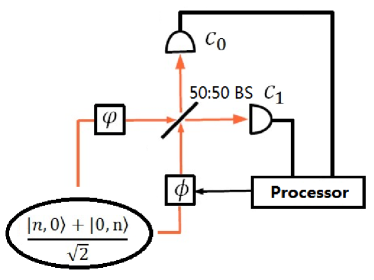
Figure 1: Measurement scheme for the unknown phase $\varphi$ with the help of the NOON state $\left(|{n,0}\rangle+|{0,n}\rangle\right)/\sqrt{2}$

To perform a phase measurement Berry et. al. Berry et al. (2009) use a sequence of NOON states $(|{n,0}\rangle+|{0,n}\rangle)/\sqrt{2}$ with $n=2^{k}$, where $k$ is varied from $K$ to $0$. These states are sent through a Mach-Zehnder interferometer as shown in Fig. 1, where the phase of the light in one arm is shifted by the unknown phase $\varphi$ and by a controllable phase $\phi$ in the other arm. The photons are detected in the two output modes $c_{0}$ and $c_{1}$ after the 50/50 beam-splitter. The detection of all photons, with measurement results $\vec{u}_{n}=\left\{u_{1},u_{2},\dots,u_{n}\right\}$ and $u_{j}\in\{0,1\}$ obeys the probability distribution

$$P(\vec{u}_{n}|\varphi)\equiv\frac{1}{2}\left\{1+(-1)^{u}\cos[n(\varphi-\phi)]\right\}$$ (1)

where $u$ is given by the parity (even or odd) of $u_{1}+u_{2}+\dots+u_{n}$. In order to explain the phase measurement scheme, we first assume that the unknown phase $\varphi$ is of the form

$$\varphi\equiv\varphi_{K}\equiv\pi\sum\limits_{k=0}^{K}\frac{a_{k}}{2^{k}}$$ (2)

with $a_{k}\in\{0,1\}$. We start with $n=2^{K}$ and $\phi=0$, which leads to the probability distribution

$$P(\vec{u}_{n}|\varphi_{K})=\frac{1}{2}\left\{1+(-1)^{u}\cos[(\pi a_{K})]\right\}.$$ (3)

which is equal to zero or unity depending on $a_{K}$ and $u$ as specified below

$$\begin{array}[]{c|c|c}&u=even&u=odd\\ \hline\cr a_{K}=0&1&0\\ a_{K}=1&0&1\end{array}$$ (4)

As a consequence, if we have measured $u$ equals an even number, we know that $a_{K}$ must be equal to zero, because for $a_{K}=1$, the probability to measure $u=even$ is zero. On the other hand, if we have measured $u$ equals odd, then we know $a_{K}=1$.

For the next measurement, we choose $n=2^{K-1}$ and $\phi=\pi a_{K}/2^{K}$ and get $a_{K-1}$ similar to $a_{K}$, and so on until we have measured all coefficients $a_{k}$.

However, in general the unknown phase $\varphi$ consist of an infinite number of coefficients and therefore, we can not measure them exactly. To determine the accuracy of this phase measurement algorithm, we discribe all measurements for different photon numbers $n$ by one POVM, given by

$$F(\hat{\varphi})\equiv|{\varphi}\rangle\langle{\varphi}|,\quad|{\varphi}\rangle\equiv\frac{1}{N_{K}}\sum\limits_{j=0}^{N_{K}}{\mkern 1.0mu\mathrm{e}\mkern 1.0mu}^{{\mkern 1.0mu\mathrm{i}\mkern 1.0mu}j\hat{\varphi}}|{j}\rangle.$$ (5)

performed on the state

$$|{\psi}\rangle\equiv\frac{1}{(N_{K}+1)^{1/2}}\sum\limits_{j=0}^{N_{K}}{\mkern 1.0mu\mathrm{e}\mkern 1.0mu}^{{\mkern 1.0mu\mathrm{i}\mkern 1.0mu}j\varphi}|{j}\rangle$$ (6)

with $N_{K}=2^{K+1}-1$.

The scaling of the algorithm depends on the phase variance $(\Delta\varphi)^{2}$ which is usually given by Holevo variance $V_{H}\equiv\mu^{-2}-1$ with $\mu\equiv|\langle e^{i\hat{\varphi}}\rangle|$. Thus the feedback phase $\phi$ should maximize $\mu$ in the system phase ($\varphi$) probability distribution. From Bayes’ theorem, the probability distribution for the system phase is then $P(\varphi|u)\propto P(\vec{u}_{n}|\varphi)$ provided that $\varphi$ is an initially completely unknown phase. Therefore, the sharpness of the phase distribution in the semiclassical case is given by Berry et al. (2009)

$$\mu=\frac{1}{2\pi}\sum_{\vec{u}_{n}}|\int e^{i\varphi}P(\vec{u}_{n}|\varphi)d\varphi|.$$ (7)

With maximized $\mu$ in the feedback process, the variance $V_{H}$ scales like the standard quantum limit for the measurement scheme described above. However, by using $M$ copies of each NOON states with $M\geq 4$ and performing $M$ measurement for each NOON state, Berry et. al. show that this modified algorithm scales as the Heisenberg limit Berry et al. (2009). This algorithm was performed experimentally Higgins et al. (2007) by using a single photon with $n$ passes through the phase shift and for $M=6$ repeated measurements for each $n$ given the system phase distribution Eq. (1).

The main ingredients of this scheme are the enhancement of the unknown phase $\varphi$ by the factor $n$ through NOON states and the interference of the unknown phase $\varphi$ with the controllable phase $\phi$. Furthermore, there are only two possibilities for $u$: zero or one, and all probabilities $P(\vec{u}_{n}|\varphi)$ add up to unity. Therefore, by knowing $P(\vec{u}_{n}|\varphi)$ for one given $\vec{u}_{n}$, we can calculate all other probabilities.

III Substitution of NOON states

Let us now analyze the substitution of NOON states by classical light as was done in Hemmer et al. (2006). We first consider a four-level atom as our point detector interacting with the classical fields illustrated in Fig. 2. In this scheme, level $|{b}\rangle$ is assumed to be the ground level. The intermediate levels $|{c_{1}}\rangle$ and $|{c_{2}}\rangle$ are highly detuned from the driving fields and we do not include the population decay rate from these levels. The population decay from the upper level $|{a}\rangle$ is denoted by $\gamma$. We assume that $|{b}\rangle\rightleftharpoons|{c_{1}}\rangle$, $|{c_{1}}\rangle\rightleftharpoons|{c_{2}}\rangle$ and $|{c_{2}}\rangle\rightleftharpoons|{a}\rangle$ are the only dipole allowed transitions.

The basic idea behind this scheme is to send two signal beams of slightly different frequencies $\nu_{\pm}$ from opposite directions and two vertically incident driving beams of frequencies $\omega_{\pm}$ as shown in Fig. 2. The excitation from level $|{a}\rangle$ to $|{b}\rangle$ can take place by either absorbing two $\nu_{+}$ signal photons and emitting one $\omega_{+}$ driving photon or absorbing two $\nu_{-}$ signal photons and emitting one $\omega_{-}$ driving photon. Any other process (such as absorbing one $\nu_{+}$ signal photon and one $\nu_{-}$ signal photon and emitting one $\omega_{+}$ driving photon or absorbing two $\nu_{-}$ signal photons and emitting one $\omega_{+}$ driving photon) would be forbidden by selection rules or be non-resonant and therefore negligible for reasonable Rabi frequencies. These two excitation branches then stimulate the $(|{2,0}\rangle+|{0,2}\rangle)/\sqrt{2}$ NOON state path correlations which is possible for super-sensitive phase measurement when we shift the phases in each branch.

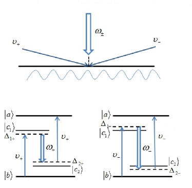
Figure 2: Two photon interference with classical light and the interaction of classical fields with the four-level atomic structure.

The two classical signal fields and one driven field interacting with the four-level atomic system are written as

$$E_{S}^{+}(x,t)\equiv\mathcal{E}_{S}{\mkern 1.0mu\mathrm{e}\mkern 1.0mu}^{{\mkern 1.0mu\mathrm{i}\mkern 1.0mu}(k_{+}x-\nu_{+}t)},$$ (8)

$$E_{S}^{-}(x,t)\equiv\mathcal{E}_{S}{\mkern 1.0mu\mathrm{e}\mkern 1.0mu}^{{\mkern 1.0mu\mathrm{i}\mkern 1.0mu}(k_{-}x-\nu_{-}t)}$$ (9)

and

$$E_{D}\equiv\mathcal{E}_{D}\left[{\mkern 1.0mu\mathrm{e}\mkern 1.0mu}^{-{\mkern 1.0mu\mathrm{i}\mkern 1.0mu}\omega_{+}t}+{\mkern 1.0mu\mathrm{e}\mkern 1.0mu}^{-{\mkern 1.0mu\mathrm{i}\mkern 1.0mu}\omega_{-}t}\right].$$ (10)

The interaction Hamiltonian in the rotating wave approximation is given by

$$\begin{split}H_{I}\equiv&\hbar\Omega_{S}\left(|{c_{1}}\rangle\langle{b}|{\mkern 1.0mu\mathrm{e}\mkern 1.0mu}^{{\mkern 1.0mu\mathrm{i}\mkern 1.0mu}\Delta_{1\pm}t+{\mkern 1.0mu\mathrm{i}\mkern 1.0mu}k_{\pm}x}+|{a}\rangle\langle{c_{2}}|{\mkern 1.0mu\mathrm{e}\mkern 1.0mu}^{{\mkern 1.0mu\mathrm{i}\mkern 1.0mu}\Delta_{2\pm}t+{\mkern 1.0mu\mathrm{i}\mkern 1.0mu}k_{\pm}x}\right)\\ &+\hbar\Omega_{D}|{c_{1}}\rangle\langle{c_{2}}|{\mkern 1.0mu\mathrm{e}\mkern 1.0mu}^{{\mkern 1.0mu\mathrm{i}\mkern 1.0mu}(\Delta_{1\pm}+\Delta_{2\pm})t}+\textrm{H.c.}.\end{split}$$ (11)

The one-photon detunings given by $\Delta_{1\pm}\equiv\omega_{c_{1}b}-\nu_{\pm}$ and $\Delta_{2\pm}\equiv\omega_{ac_{2}}-\nu_{\pm}$ are much larger compared with $1/t$ so that no atom will be excited to the intermediate levels. The three-photon resonance condition, $\omega_{ab}+\omega_{\pm}=2\nu_{\pm}$, is considered when deriving the interaction Hamiltonian.

We consider the atomic system as a narrow bandwidth detector Hemmer et al. (2006) for which the lifetime $1/\gamma$ in the excited level $|{a}\rangle$ is longer than the detecting time $t$. In the perturbative regime, $|\Delta_{j\pm}t|\gg 1$, the amplitude of excitation from $|{b}\rangle$ to $|{a}\rangle$ is given to the lowest order by the three-photon process Scully and Zubairy (1997):

$$a^{(1)}(x,t) = (-\frac{{\mkern 1.0mu\mathrm{i}\mkern 1.0mu}}{\hbar})^{3}\int_{0}^{t}dt_{1}\int_{0}^{t_{1}}dt_{2}\int_{0}^{t_{2}}dt_{3}\langle{a}|\mathnormal{H_{I}(x,t_{1})}\mathnormal{H_{I}(x,t_{2})}\mathnormal{H_{I}(x,t_{3})}|{b}\rangle$$ (12)

$$= {\mkern 1.0mu\mathrm{i}\mkern 1.0mu}\Omega_{S}^{2}\Omega_{D}t\left[\left(\frac{e^{{\mkern 1.0mu\mathrm{i}\mkern 1.0mu}2k_{+}x}}{\Delta_{1+}\Delta_{2+}}+\frac{e^{{\mkern 1.0mu\mathrm{i}\mkern 1.0mu}2k_{-}x}}{\Delta_{1-}\Delta_{2-}}\right)+\left(\frac{(e^{-{\mkern 1.0mu\mathrm{i}\mkern 1.0mu}2\delta t}-1)e^{{\mkern 1.0mu\mathrm{i}\mkern 1.0mu}2k_{+}x}}{\Delta_{1+}(\Delta_{2+}+2\delta)(-{\mkern 1.0mu\mathrm{i}\mkern 1.0mu}2\delta t)}+\frac{(e^{{\mkern 1.0mu\mathrm{i}\mkern 1.0mu}2\delta t}-1)e^{{\mkern 1.0mu\mathrm{i}\mkern 1.0mu}2k_{-}x}}{\Delta_{1-}(\Delta_{2-}-2\delta)({\mkern 1.0mu\mathrm{i}\mkern 1.0mu}2\delta t)}\right)\right.$$

$$+ \left.\left(\frac{e^{{\mkern 1.0mu\mathrm{i}\mkern 1.0mu}\delta t}-1}{\Delta_{1-}(\Delta_{2-}-2\delta)({\mkern 1.0mu\mathrm{i}\mkern 1.0mu}\delta t)}+\frac{e^{{\mkern 1.0mu\mathrm{i}\mkern 1.0mu}\delta t}-1}{\Delta_{1+}\Delta_{2+}({\mkern 1.0mu\mathrm{i}\mkern 1.0mu}\delta t)}+\frac{e^{-{\mkern 1.0mu\mathrm{i}\mkern 1.0mu}\delta t}-1}{\Delta_{1-}\Delta_{2-}(-{\mkern 1.0mu\mathrm{i}\mkern 1.0mu}\delta t)}+\frac{e^{-{\mkern 1.0mu\mathrm{i}\mkern 1.0mu}\delta t}-1}{\Delta_{1+}(\Delta_{2+}+2\delta)(-{\mkern 1.0mu\mathrm{i}\mkern 1.0mu}\delta t)}\right)e^{{\mkern 1.0mu\mathrm{i}\mkern 1.0mu}(k_{+}+k_{-})x}\right],$$

where $\delta\equiv\nu_{+}-\nu_{-}=\Delta_{j-}-\Delta_{j+}$ represents the frequency difference between the two signal beams. The physical meaning of this amplitude of excitation is the following: the first term in the square brackets represents resonant three-photon process from each channel; the second and the third terms are off resonant terms by interchanging one driving photon $\omega_{\pm}$ and one signal photon $\nu_{\pm}$ respectively from the resonant three-photon process between the two channels. Each of the non-resonant terms are multiplied by either $\frac{e^{\pm{\mkern 1.0mu\mathrm{i}\mkern 1.0mu}\delta t}-1}{\pm{\mkern 1.0mu\mathrm{i}\mkern 1.0mu}\delta t}$ or $\frac{e^{\pm{\mkern 1.0mu\mathrm{i}\mkern 1.0mu}2\delta t}-1}{\pm{\mkern 1.0mu\mathrm{i}\mkern 1.0mu}2\delta t}$. For $\delta t\gg 1$,

$$|\frac{e^{\pm{\mkern 1.0mu\mathrm{i}\mkern 1.0mu}j\delta t}-1}{\pm{\mkern 1.0mu\mathrm{i}\mkern 1.0mu}j\delta t}|\leq\frac{2}{j\delta t}\ll 1\quad(j=1,2),$$ (13)

the contribution from the non-resonant terms is in general proportional to $1/(\delta t/2)$.

Under the condition $\delta t\gg 1$ and $\gamma t<1$, the only two significant terms in the first order perturbation theory will be the resonant term for which the same beam, $+$ or $-$, contributes twice. Therefore, the amplitude of excitation $a^{(1)}(x,t)$ is given by

$$a^{(1)}(x,t)\equiv{\mkern 1.0mu\mathrm{i}\mkern 1.0mu}\Omega_{S}^{2}\Omega_{D}t\left(\frac{{\mkern 1.0mu\mathrm{e}\mkern 1.0mu}^{{\mkern 1.0mu\mathrm{i}\mkern 1.0mu}2k_{+}x}}{\Delta_{1+}\Delta_{2+}}+\frac{{\mkern 1.0mu\mathrm{e}\mkern 1.0mu}^{{\mkern 1.0mu\mathrm{i}\mkern 1.0mu}2k_{-}x}}{\Delta_{1-}\Delta_{2-}}\right).$$ (14)

For $\Delta_{1+}\Delta_{2+}\approx\Delta_{1-}\Delta_{2-}\equiv\Delta_{1}\Delta_{2}$ the probability $P_{a}(x,t)$ to find the atom in the state $|{a}\rangle$ is given by

$$P_{a}(x,t)=2\left|\frac{\Omega_{S}^{2}\Omega_{D}t}{\Delta_{1}\Delta_{2}}\right|^{2}\left[1+\cos(2k_{+}x-2k_{-}x)\right].$$ (15)

Note that this perturbation theory is only valid when the effective Rabi frequency $\frac{\Omega_{S}^{2}\Omega_{D}}{\Delta_{1}\Delta_{2}}\ll 1/t$ Hemmer et al. (2006). This probability shows an increased resolution by absorbing two photons each time from each channel.

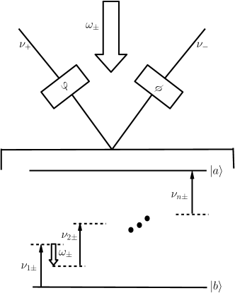
Figure 3: The two signal fields with frequencies $\nu_{+}$ and $\nu_{-}$ are shifted by the unknown phase $\varphi$ and the controllable phase $\phi$, respectively. The drive fields $\omega_{\pm}$ assist a directional resonance of $n$ photon absorption.

This scheme can be generalized to an atom with $n$ intermediate levels, where the two signal fields are replaced by two bunches of signal fields, which obey the following resonance condition

$$\omega_{ab}=\sum\limits_{j=0}^{n}\nu_{j\pm}-(n-1)\omega_{\pm}.$$ (16)

As explained above, under the condition $\delta t\gg 1$ and $\gamma t<1$, any interchange of photons between the two excitation branches will result in a loss of resonance and any non-resonant processes can be neglected. This relation ensures that the atom absorbs $n$ photons from one branch of the signal beams ($\nu_{+}$ or $\nu_{-}$) and emits $(n-1)$ photons of the frequency $\omega_{+}$ or $\omega_{-}$. By applying a phase shift $\varphi$ on one of the signal fields and by $\phi$ on the other as illustrated in Fig. 3 and assuming that $(k_{+}-k_{-})x=0$, we obtain

$$P_{a}(t|\varphi,\phi)=2\Omega_{eff}^{2}t^{2}\left\{1+\cos\left[n(\varphi-\phi)\right]\right\}$$ (17)

with

$$\Omega_{eff}\equiv\frac{\Omega_{S}^{n}\Omega_{D}^{n-1}}{\prod\limits_{j=1}^{n-1}\Delta_{2j-1}\Delta_{2j}},$$ (18)

and the generalized perturbative regime is $\Omega_{eff}t\ll 1$. Therefore, the probability distribution $P_{a}$ behaves the same way as the probability distribution Eq. (1) of a NOON state used for measuring the unknown phase $\varphi$, but only with the factor $u$ being fixed to an even number. However, if we know the result of the function

$$1+(-1)^{u}\cos[n(\varphi-\phi)]$$ (19)

for $u=even$, we are able to calculate it for $u=odd$, as we have explained already in Sec. II. As a consequence, we can use $P_{a}$ in the same way as Berry et. al. use $P(\vec{u}_{n}|\varphi)$ to estimate the unknown phase $\varphi$. This is the main result of our paper.

In the quantum phase measurement with entangled states, the generation and detection processes of entangled states are required separately. On the other hand, in our scheme, the multiphoton frequency-selective measurement using classical light generates and detects an effective NOON state simultaneously, which makes it easier to implement the scheme experimentally.

Another difference between the two schemes is that the measurement result of the Mach-Zehnder interferometer, which is $u$ and not the probability distribution $P(\vec{u}_{n}|\varphi)$, is restricted to $u$ equals to even or odd. We note that in our approach, we measure the excitation rate $R^{(2n-1)}\equiv\frac{d}{dt}P_{a}(t|\varphi,\phi)$ , which can assume every number between zero and the maximal excitation rate given by $R^{(2n-1)}_{\text{max}}\equiv 8\Omega_{eff}^{2}t$. This gives us more information about the unknown phase $\varphi$. However, if we want to follow the phase-measurement scheme described in Berry et al. (2009) exactly, then an excitation rate larger than half the maximal rate would correspond to $u=even$, and an excitation rate smaller than half the maximal rate would correspond to $u=odd$.

IV Detection Rate Scaling and Error Estimation

IV.1 Detection Rate Scaling

Now we investigate the scaling of maximal excitation rate in our scheme compared with the one in Berry et al. (2009), and obtain the accuracy in supersensitive phase measurement of our scheme.

The phase-measurement scheme described in Berry et al. (2009) is a realization of the POVM

$$F(\hat{\varphi})\equiv|{\varphi}\rangle\langle{\varphi}|,\quad|{\varphi}\rangle\equiv\frac{1}{N_{K}}\sum\limits_{j=0}^{N_{K}}{\mkern 1.0mu\mathrm{e}\mkern 1.0mu}^{{\mkern 1.0mu\mathrm{i}\mkern 1.0mu}j\hat{\varphi}}|{j}\rangle$$ (20)

performed on the state

$$|{\psi}\rangle\equiv\frac{1}{(N_{K}+1)^{M/2}}\left(\sum\limits_{j=0}^{N_{K}}{\mkern 1.0mu\mathrm{e}\mkern 1.0mu}^{{\mkern 1.0mu\mathrm{i}\mkern 1.0mu}j\varphi}|{j}\rangle\right)^{\otimes M}$$ (21)

Here, $N_{K}$ is given by $N_{K}=2^{K+1}-1$. Therefore the number of resources is given by $N\equiv N_{K}\cdot M$. If the reference phase $\phi$ is chosen adaptively and for $M\geq 4$, this phase-measurement algorithm scales like the Heisenberg limit.

Our proposed scheme is just another realization of the same POVM and therefore also scales like the Heisenberg limit.

In order to find whether it is better to realize with NOON-states or classical light, we investigate the resources and problems needed for our realization of the POVM and compare it to the NOON-state approach. For the NOON-state realization, we have to create the NOON states $(|{2,0}\rangle+|{0,2}\rangle)/\sqrt{2}$, $(|{2^{2},0}\rangle+|{0,2^{2}}\rangle)/\sqrt{2}$, $\cdots$, $(|{2^{K},0}\rangle+|{0,2^{K}}\rangle)/\sqrt{2}$ which is very difficult, and two multiphoton detectors with high efficiency. If the probability of detecting one photon is given by $\eta$, then the probability of detecting all photons of the NOON state $(|{n,0}\rangle+|{0,n}\rangle)/\sqrt{2}$ is given by $\eta^{n}$ Scully and Zubairy (1997); Tsang (2007). As a consequence, the detection rate decreases exponentially with $n$. As mentioned above, Steuernagel pointed out Steuernagel (2004) the detection rate of entangled photons arriving at one point will be even smaller since the photons are spatially unconstrained. Furthermore, the detectors $c_{0}$ and $c_{1}$ need to detect and discriminate between the states $|{0}\rangle$, $|{1}\rangle,\dots$, ${|{n}\rangle}$. In Berry et al. (2009) the authors do not explain how to achieve this task.

For the realization with classical light, we need an atom with multi-level structure. The maximal excitation rate scales like

$$R^{2n-1}_{max}=2\left|\frac{\Omega_{S}\Omega_{D}}{\Delta_{\pm}^{2}}\right|^{2n}\left|\frac{2\Delta_{\pm}^{2}}{\Omega_{D}}\right|^{2}t=2\left|\frac{2\Delta_{\pm}^{2}}{\Omega_{D}}\right|^{2}\eta^{n}t$$ (22)

with

$$\eta\equiv\left|\frac{\Omega_{S}\Omega_{D}}{\Delta_{\pm}^{2}}\right|^{2}.$$ (23)

As a consequence, the excitation rate decreases exponentially with $n$ similar to the photon detection rate of the NOON-state approach. However, since a large number of photons exist in the classical light, although spatially unconstrained there are enough photons to arrive at one point to excite the atom (the detector). Therefore, the spatial distribution of the photons does not affect the excitation rate in our case.

IV.2 Error Estimation

Now we derive in the following possible errors in our scheme from resonant higher-order terms and from non-resonant terms in a general case.

For large $n$, strong Rabi frequencies can be used to improve the excitation rate. We find a tradeoff in using strong Rabi frequencies such that resonant higher order terms and non-resonant terms can not be neglected. First, we obtain for the second-order resonant term from perturbation theory Scully and Zubairy (1997) (which corresponds to a five-photon process) as Rabi frequencies increase

$$a^{(2)}(t|\varphi,\phi) = (-\frac{i}{\hbar})^{5}\int\int\int\int\int dt^{5}\langle{a}|\mathnormal{H_{I}(\varphi,\phi,t_{1})}\mathnormal{H_{I}(\varphi,\phi,t_{2})}\mathnormal{H_{I}(\varphi,\phi,t_{3})}\mathnormal{H_{I}(\varphi,\phi,t_{4})}\mathnormal{H_{I}(\varphi,\phi,t_{5})}|{b}\rangle$$ (24)

$$\equiv i\Omega_{S}^{2}\Omega_{D}t\left(\frac{{\mkern 1.0mu\mathrm{e}\mkern 1.0mu}^{2{\mkern 1.0mu\mathrm{i}\mkern 1.0mu}\varphi}}{\Delta_{1+}\Delta_{2+}}+\frac{{\mkern 1.0mu\mathrm{e}\mkern 1.0mu}^{2{\mkern 1.0mu\mathrm{i}\mkern 1.0mu}\phi}}{\Delta_{1-}\Delta_{2-}}\right)\times({\mkern 1.0mu\mathrm{i}\mkern 1.0mu}r_{1}-{\mkern 1.0mu\mathrm{i}\mkern 1.0mu}r_{2}-r_{3})$$

with

$$r_{1}\equiv\frac{\Omega_{S}^{2}t}{\Delta_{1+}}+\frac{\Omega_{S}^{2}t}{\Delta_{1-}},\quad r_{2}\equiv\frac{\Omega_{S}^{2}t}{\Delta_{2+}}+\frac{\Omega_{S}^{2}t}{\Delta_{2-}}$$ (25)

and

$$r_{2} \equiv \frac{\Omega_{D}^{2}}{\Delta_{1+}\Delta_{2+}}+\frac{\Omega_{D}^{2}}{\Delta_{1-}\Delta_{2-}}$$ (26)

$$+\frac{\Omega_{D}^{2}}{\Delta_{1\pm}(\Delta_{2\mp}\pm\delta)}+\frac{\Omega_{D}^{2}}{(\Delta_{1\mp}\pm\delta)\Delta_{2\pm}}.$$

Here $\mathnormal{H_{I}(\varphi,\phi,t)}$ is obtained from Eq. (11) by replacing $k_{\pm}x$ with $\varphi$ and $\phi$ respectively. The second-order result is obtained by multiplying Rabi oscillation factors ($r_{j}$), which describe additional two-photon processes between intermediate levels, to the first order contribution $a^{(1)}(x,t)$ in Eq. (14). The Rabi oscillation factors are the tendency of resonant higher order terms, and therefore they have to be much smaller than unity for perturbation theory to work. We solve this tradeoff by choosing opposite one-photon detunings, $\Delta_{j+}=-\Delta_{j-}$, such that $r_{1}=r_{2}=0$ while signal Rabi frequency $|\Omega_{S}^{2}t/\Delta_{\pm}|$ can be large. We choose $\Omega_{D}^{2}\ll|\Delta_{(2j-1)\pm}\Delta_{2j\pm}|$ to suppress the other Rabi oscillation factor $r_{3}$. Therefore, under the above conditions of Rabi frequencies and one-photon detunings, resonant higher-order terms can be neglected and the excitation rate can be improved.

We discussed the non-resonant terms of a four-level atomic system in the previous section and now we extend this to a $2n-$level atomic system. In general, the non-resonant terms result from an absorption of $n-k$ photons of frequency $\nu_{+}$ and $k$ photons of frequency $\nu_{-}$. The leading term comes from the exchange of one photon, and therefore the probability amplitude of the state $|{a}\rangle$ is given by

$$a(t|\varphi,\phi) = \Omega_{eff}t\left[{\mkern 1.0mu\mathrm{e}\mkern 1.0mu}^{{\mkern 1.0mu\mathrm{i}\mkern 1.0mu}n\varphi}+{\mkern 1.0mu\mathrm{e}\mkern 1.0mu}^{{\mkern 1.0mu\mathrm{i}\mkern 1.0mu}n\phi}+n\frac{{\mkern 1.0mu\mathrm{e}\mkern 1.0mu}^{{\mkern 1.0mu\mathrm{i}\mkern 1.0mu}\delta t}-1}{{\mkern 1.0mu\mathrm{i}\mkern 1.0mu}\delta t}\right.$$ (27)

$$\left.\times\left({\mkern 1.0mu\mathrm{e}\mkern 1.0mu}^{{\mkern 1.0mu\mathrm{i}\mkern 1.0mu}(n-1)\varphi+{\mkern 1.0mu\mathrm{i}\mkern 1.0mu}\phi}+{\mkern 1.0mu\mathrm{e}\mkern 1.0mu}^{{\mkern 1.0mu\mathrm{i}\mkern 1.0mu}\varphi+{\mkern 1.0mu\mathrm{i}\mkern 1.0mu}(n-1)\phi}\right)\right]$$

with $\Omega_{eff}\equiv\Omega_{S}^{n}\Omega_{D}^{n-1}/\Delta_{\pm}^{2n-2}$. Providing $n\sin(\delta t)/(\delta t)\ll 1$, the probability to find the atom in the excited state is given by

$$P(t|\varphi,\phi) = 2(\Omega_{eff}t)^{2}\left\{1+\cos[n(\varphi-\phi)]+4\frac{n\sin(\delta t)}{\delta t}\right.$$ (28)

$$\left.\times\cos[\frac{n}{2}(\varphi-\phi)]\cos[\frac{n-2}{2}(\varphi-\phi)]\right\}.$$

Assuming, that the unknown phase $\varphi$ is given by $\varphi\equiv\pi(\varphi_{0}+\varphi_{1}/2+\varphi_{2}/2^{2}+\dots)$ with $\varphi_{n}\in\{0,1\}$ and by applying the phase-measurement algorithm described in Berry et al. (2009), the accuracy of obtaining the supersensitive phase $\varphi_{n}$ with a detection process involving $n$ photons of frequency $\nu_{\pm}$ is given by

$$\frac{1}{1+\frac{2n\sin(\delta t)}{\delta t}}<1.$$ (29)

Despite these possible errors, we think our realization of the phase measurement is more useful, than the one using NOON states, because we think it is easier to find an atom with the right level structure than to create NOON states with many photons and to find the appropriate detector.

V Discussion and conclusion

We have shown in this paper that the substitution of NOON states by classical light in the multiphoton frequency-selective measurement (as suggested for subwavelength lithography in Hemmer et al. (2006)) is applicable to the phase-measurement scheme described in Berry et al. (2009) to obtain an accurate phase-measurement limit. We have found that our scheme is easier to implement in two ways compared to that in Berry et al. (2009). The first advantage is that the multiphoton process using classical light in our scheme generates and detects a NOON state at the same time, while the quantum phase measurement with entangled states requires the generation and detection of entangled states separately. The second advantage is that, in our scheme, the multiphoton absorption rate with classical light is not affected by the spatial distribution of the photons as that in the scheme using entangled states. Therefore, we conclude that our scheme with multiphoton frequency-selective measurement using classical light provides an alternative and better adaptive phase measurement method.

References

- Caves (1981) C. M. Caves, Phys. Rev. D. 23, 1693 (1981).
- Yurke et al. (1986) B. Yurke, S. L. McCall, and J. R. Klauder, Phys. Rev. A 33, 4033 (1986).
- Sanders et al. (1995) B. C. Sanders, and G. J. Milburn, Phys. Rev. Lett. 75, 2944 (1995).
- Lee et al. (2002) H. Lee, P. Kok, and J. P. Dowling, J. Mod. Opt. 49, 2325 (2002).
- Boto et al. (2000) A. N. Boto, P. Kok, D. S. Abrams, S. L. Braunstein, C. P. Williams, and J. P. Dowling, Phys. Rev. Lett. 85, 2733 (2000).
- Wei et al. (2011) R. Wei, B. Zhao, Y. Deng, Y.-A. Chen, and J.-W. Pan, Phys. Rev. A 83, 063623 (2011).
- Berry et al. (2009) D. W. Berry, B. L. Higgins, S. D. Bartlett, M. W. Mitchell, G. J. Pryde, and H. M. Wiseman, Phys. Rev. A. 80, 052114 (2009).
- Higgins et al. (2007) B. L. Higgins, D. W. Berry, S. D. Bartlett, H. M. Wiseman, and G. J. Pryde, Nature 450, 393 (2007).
- Xiang et al. (2010) G. Y. Xiang, B. L. Higgins, D. W. Berry, H. W. Wiseman, and G. J. Pryde, Nature 450, 43 (2010).
- Steuernagel (2004) O. Steuernagel, J. Opt. B:Quantum Semiclass. Opt. 6, S606 (2004).
- Hemmer et al. (2006) P. R. Hemmer, A. Muthukrishnan, M. O. Scully, and M. S. Zubairy, Phys. Rev. Lett. 96, 163603 (2006).
- Haroche and Hartmann (1972) S. Haroche and F. Hartmann, Phys. Rev. A 6, 1280 (1972).
- Kyrola and Stenholm (1977) E. Kyrola and S. Stenholm, Opt. Commun. 22, 123 (1977).
- Berman and Ziegler (1977) P. R. Berman and J. Ziegler, Phys. Rev. A 15, 2042 (1977).
- Walther et al. (2004) P. Walther, J.-W. Pan, M. Aspelmeyer, R. Ursin, S. Gasparoni, and A. Zeilinger, Nature (London) 429, 158 (2004).
- Mitchell et al. (2004) M. Mitchell, J. Lundeen, and A. Steinberg, Nature (London) 429, 161 (2004).
- Nagata et al. (2007) T. Nagata, R. Okamoto, J. L. O’Brien, K. Sasaki, and S. Takeuchi, Science 316, 726 (2007).
- Resch et al. (2007) K. J. Resch, K. L. Pregnell, R. Prevedel, A. Gilchrist, G. J. Pryde, J. L. O’Brien, and A. G. White, Phys. Rev. Lett. 98, 223601 (2007).
- Chen et al. (2010) Y.-A. Chen, X.-H. Bao, Z.-S. Yuan, S. Chen, B. Zhao, and J.-W. Pan, Phys. Rev. Lett. 104, 043601 (2010).
- D’Angelo et al. (2001) M. D’Angelo, M. V. Chekhova, and Y. Shih, Phys. Rev. Lett. 87, 013602 (2001).
- Scully and Zubairy (1997) M. O. Scully and M. S. Zubairy, Quantum Optics (Cambridge University Press, Cambridge, 1997).
- Tsang (2007) M. Tsang, Phys. Rev. A 75, 043813 (2007).
- Higgins et al. (2009) B. L. Higgins, D. W. Berry, S. D. Bartlett, H. M. Mitchell, W. H. M., and P. G. J., New J. Phys. 11, 073023 (2009).