ANOVA for longitudinal data with missing values

Abstract

We carry out ANOVA comparisons of multiple treatments for longitudinal studies with missing values. The treatment effects are modeled semiparametrically via a partially linear regression which is flexible in quantifying the time effects of treatments. The empirical likelihood is employed to formulate model-robust nonparametric ANOVA tests for treatment effects with respect to covariates, the nonparametric time-effect functions and interactions between covariates and time. The proposed tests can be readily modified for a variety of data and model combinations, that encompasses parametric, semiparametric and nonparametric regression models; cross-sectional and longitudinal data, and with or without missing values.

T1Supported by NSF Grants SES-0518904, DMS-06-04563 and DMS-07-14978.

and

1 Introduction

Randomized clinical trials and observational studies are often used to evaluate treatment effects. While the treatment versus control studies are popular, multi-treatment comparisons beyond two samples are commonly practised in clinical trails and observational studies. In addition to evaluate overall treatment effects, investigators are also interested in intra-individual changes over time by collecting repeated measurements on each individual over time. Although most longitudinal studies are desired to have all subjects measured at the same set of time points, such “balanced” data may not be available in practice due to missing values. Missing values arise when scheduled measurements are not made, which make the data “unbalanced.” There is a good body of literature on parametric, nonparametric and semiparametric estimation for longitudinal data with or without missing values. This includes Liang and Zeger (1986), Laird and Ware (1982), Wu, Chiang and Hoover (1998), Wu and Chiang (2000), Fitzmaurice, Laird and Ware (2004) for methods developed for longitudinal data without missing values; and Little and Rubin (2002), Little (1995), Laird (2004), Robins, Rotnitzky and Zhao (1995) for missing values.

The aim of this paper is to develop ANOVA tests for multi-treatment comparisons in longitudinal studies with or without missing values. Suppose that at time $t$, corresponding to $k$ treatments there are $k$ mutually independent samples,

$$\{(Y_{1i}(t),X^{\tau}_{1i}(t))\}_{i=1}^{n_{1}},\ldots,\{(Y_{ki}(t),X^{\tau}_{ki}(t))\}_{i=1}^{n_{k}},$$

where the response variable $Y_{ji}(t)$ and the covariate $X_{ji}(t)$ are supposed to be measured at time points $t=t_{ji1},\ldots,t_{jiT_{j}}$. Here $T_{j}$ is the fixed number of scheduled observations for the $j$th treatment. However, $\{Y_{ji}(t),X^{\tau}_{ji}(t)\}$ may not be observed at some times, resulting in missing values in either the response $Y_{ji}(t)$ or the covariates $X_{ji}(t)$.

We consider a semiparametric regression model for the longitudinal data

$$Y_{ji}(t)=X_{ji}^{\tau}(t)\beta_{j0}+M^{\tau}(X_{ji}(t),t)\gamma_{j0}+g_{j0}(t)+\varepsilon_{ji}(t),$$

(1)

$$\eqntext{j=1,2,\ldots,k,}$$ (2)

where $M(X_{ji}(t),t)$ are known functions of $X_{ji}(t)$ and time $t$ representing interactions between the covariates and the time, $\beta_{j0}$ and $\gamma_{j0}$ are $p$- and $q$-dimensional parameters, respectively, $g_{j0}(t)$ are unknown smooth functions representing the time effect, and $\{\varepsilon_{ji}(t)\}$ are residual time series. Such a semiparametric model may be viewed as an extended partially linear model. The partially linear model has been used for longitudinal data analysis; see Zeger and Diggle (1994), Zhang et al. (1998), Lin and Ying (2001), Wang, Carroll and Lin (2005). Wu, Chiang and Hoover (1998) and Wu and Chiang (2000) proposed estimation and confidence regions for a semiparametric varying coefficient regression model. Despite a body of works on estimation for longitudinal data, analysis of variance for longitudinal data have attracted much less attention. A few exceptions include Forcina (1992) who proposed an ANOVA test in a fully parametric setting; and Scheike and Zhang (1998) who considered a two sample test in a fully nonparametric setting.

In this paper, we propose ANOVA tests for differences among the $\beta_{j0}$’s and the baseline time functions $g_{j0}$’s, respectively, in the presence of the interactions. The ANOVA statistics are formulated based on the empirical likelihood [Owen (1988, 2001)], which can be viewed as a nonparametric counterpart of the conventional parametric likelihood. Despite its not requiring a fully parametric model, the empirical likelihood enjoys two key properties of a conventional likelihood, the Wilks’ theorem [Owen (1990), Qin and Lawless (1994), Fan and Zhang (2004)] and Bartlett correction [DiCicco, Hall and Romano (1991), Chen and Cui (2006)]; see Chen and Van Keilegom (2009) for an overview on the empirical likelihood for regression. This resemblance to the parametric likelihood ratio motivates us to consider using empirical likelihood to formulate ANOVA test for longitudinal data in nonparametric situations. This will introduce a much needed model-robustness in the ANOVA testing.

Empirical likelihood has been used in studies for either missing or longitudinal data. Wang and Rao (2002), Wang, Linton and Härdle (2004) considered an empirical likelihood inference with a kernel regression imputation for missing responses. Liang and Qin (2008) treated estimation for the partially linear model with missing covariates. For longitudinal data, Xue and Zhu (2007a, 2007b) proposed a bias correction method to make the empirical likelihood statistic asymptotically pivotal in a one sample partially linear model; see also You, Chen and Zhou (2006) and Huang, Qin and Follmann (2008).

In this paper, we propose three empirical likelihood based ANOVA tests for the equivalence of the treatment effects with respect to (i) the covariate $X_{ji}$; (ii) the interactions $M(X_{ji}(t),t)$ and (iii) the time effect functions $g_{j0}(\cdot)$’s, by formulating empirical likelihood ratio test statistics. It is shown that for the proposed ANOVA tests for the covariates effects and the interactions, the empirical likelihood ratio statistics are asymptotically chi-squared distributed, which resembles the conventional ANOVA statistics based on parametric likelihood ratios. This is achieved without parametric model assumptions for the residuals in the presence of the nonparametric time effect functions and missing values. Hence, the empirical likelihood ANOVA tests have the needed model-robustness. Another attraction of the proposed ANOVA tests is that they encompass a set of ANOVA tests for a variety of data and model combinations. Specifically, they imply specific ANOVA tests for both cross-sectional and longitudinal data; for parametric, semiparametric and nonparametric regression models; and with or without missing values.

The paper is organized as below. In Section 2, we describe the model and the missing value mechanism. Section 3 outlines the ANOVA test for comparing treatment effects due to the covariates: whereas the tests regarding interaction are proposed in Section 5. Section 4 considers ANOVA test for the nonparametric time effects. The bootstrap calibration to the ANOVA test on the nonparametric part is outlined in Section 6. Section 7 reports simulation results. We applied the proposed ANOVA tests in Section 8 to analyze an HIV-CD4 data set. Technical assumptions are presented in the Appendix. All the technical proofs to the theorems are reported in a supplement article [Chen and Zhong (2010)].

2 Models, hypotheses and missing values

For the $i$th individual of the $j$th treatment, the measurements taken at time $t_{jim}$ follow a semiparametric model

$$Y_{ji}(t_{jim}) = X^{\tau}_{ji}(t_{jim})\beta_{j0}+M^{\tau}(X_{ji}(t_{jim}),t_{jim})\gamma_{j0}$$

$${}+g_{j0}(t_{jim})+\varepsilon_{ji}(t_{jim}),$$

for $j=1,\ldots,k$, $i=1,\ldots,n_{j}$, $m=1,\ldots,T_{j}$. Here $\beta_{j0}$ and $\gamma_{j0}$ are unknown $p$- and $q$-dimensional parameters and $g_{j0}(t)$ are unknown functions representing the time effects of the treatments. The time points $\{t_{jim}\}_{m=1}^{T_{j}}$ are known design points. For ease of notation, we write $(Y_{jim},X_{jim}^{\tau},M_{jim}^{\tau})$ to denote $(Y_{ji}(t_{jim}),X_{ji}^{\tau}(t_{jim}),M^{\tau}(X_{ji}(t_{jim}),t_{jim}))$. Also, we will use $\mathbb{X}_{jim}^{\tau}=(X_{jim}^{\tau},M_{jim}^{\tau})$ and $\mathbb{\xi}_{j}^{\tau}=(\beta_{j}^{\tau},\gamma_{j}^{\tau})$. For each individual, the residuals $\{\epsilon_{ji}(t)\}$ satisfy $E\{\varepsilon_{ji}(t)|X_{ji}(t)\}=0$, $\operatorname{Var}\{\varepsilon_{ji}(t)|X_{ji}(t)\}=\sigma^{2}_{j}(t)$ and

$$\operatorname{Cov}\{\varepsilon_{ji}(t),\varepsilon_{ji}(s)|X_{ji}(t),X_{ji}(s)\}=\rho_{j}(s,t)\sigma_{j}(t)\sigma_{j}(s),$$

where $\rho_{j}(s,t)$ is the conditional correlation coefficient between two residuals at two different times. And the residual time series $\{\epsilon_{ji}(t)\}$ from different subjects and different treatments are independent. Without loss of generality, we assume $t,s\in[0,1]$. For the purpose of identifying $\beta_{j0}$, $\gamma_{j0}$ and $g_{j0}(t)$, we assume

$$(\beta_{j0},\gamma_{j0},g_{j0})=\mathop{\arg\min}_{(\beta_{j},\gamma_{j},g_{j})}\frac{1}{n_{j}T_{j}}\sum_{i=1}^{n_{j}}\sum_{m=1}^{T_{j}}E\{Y_{jim}-X^{\tau}_{jim}\beta_{j}-M^{\tau}_{jim}\gamma_{j}-g_{j}(t_{jim})\}^{2}.$$

We also require that $\frac{1}{n_{j}T_{j}}\sum_{i=1}^{n_{j}}\sum_{m=1}^{T_{j}}E(\widetilde{\mathbb{X}}_{jim}\widetilde{\mathbb{X}}_{jim}^{\tau})>0$, where $\widetilde{\mathbb{X}}_{jim}=\mathbb{X}_{jim}-E(\mathbb{X}_{jim}|t_{jim})$. This condition also rules out $M(X_{ji}(t),t)$ being a pure function of $t$, and hence it has to be genuine interaction. For the same reason, the intercept in model (2) is absorbed into the nonparametric part $g_{j0}(t)$.

As commonly exercised in the partially linear model [Speckman (1988); Linton and Nielsen (1995)], there is a secondary model for the covariate $X_{jim}$:

$$X_{jim}=h_{j}(t_{jim})+u_{jim},$$

(4)

$$\eqntext{j=1,2,\ldots,k,i=1,\ldots,n_{j},m=1,\ldots,T_{j},}$$ (5)

where $h_{j}(\cdot)$’s are $p$-dimensional smooth functions with continuous second derivatives, the residual $u_{jim}=(u_{jim}^{1},\ldots,u_{jim}^{p})^{\tau}$ satisfy $E(u_{jim})=0$ and $u_{jl}$ and $u_{jk}$ are independent for $l\neq k$, where $u_{jl}=(u_{jl1},\ldots,u_{jlT_{j}})$. By the identification condition given above, the covariance matrix of $u_{jim}$ is assumed to be finite and positive definite.

We are interested in testing three ANOVA hypotheses. The first one is on the treatment effects with respect to the covariates:

$$H_{0a}\dvtx\beta_{10}=\beta_{20}=\cdots=\beta_{k0}\quad\mbox{vs.}\quad H_{1a}\dvtx\beta_{i0}\neq\beta_{j0}\qquad\mbox{for some }i\neq j.$$

The second one is regarding the time effect functions:

$$H_{0b}\dvtx g_{10}(\cdot)=\cdots=g_{k0}(\cdot)\quad\mbox{vs.}\quad H_{1b}\dvtx g_{i0}(\cdot)\neq g_{j0}(\cdot)\qquad\mbox{for some }i\neq j.$$

The third one is on the existence of the interaction $H_{0c}\dvtx\gamma_{j0}=0$ and $H_{1c}\dvtx\break\gamma_{j0}\neq 0$. And the last one is the ANOVA test for

$$H_{0d}\dvtx\gamma_{10}=\gamma_{20}=\cdots=\gamma_{k0}\quad\mbox{vs.}\quad H_{1d}\dvtx\gamma_{i0}\neq\gamma_{j0}\qquad\mbox{for some }i\neq j.$$

Let $X_{ji}=\{X_{ji0},\ldots,X_{jiT_{j}}\}$ and $Y_{ji}=\{Y_{ji0},\ldots,Y_{jiT_{j}}\}$ be the complete time series of the covariates and responses of the $(j,i)$th subject (the $i$th subject in the $j$th treatment), and $\accentset{\leftharpoonup}{Y}_{jit,d}=\{Y_{ji(t-d)},\ldots,Y_{ji(t-1)}\}$ and $\accentset{\leftharpoonup}{X}_{jit,d}=\{X_{ji(t-d)},\ldots,X_{ji(t-1)}\}$ be the past $d$ observations at time $t$ for a positive integer $d\leq\min_{j}\{T_{j}\}$. For $t<d$, we set $d=t-1$.

Define the missing value indicator $\delta_{jit}=1$ if $(X^{\tau}_{jit},Y_{jit})$ is observed and $\delta_{jit}=0$ if $(X^{\tau}_{jit},Y_{jit})$ is missing. Here, we assume $X_{jit}$ and $Y_{jit}$ are either both observed or both missing. This simultaneous missingness of $X_{jit}$ and $Y_{jit}$ is for the ease of mathematical exposition. We also assume that $\delta_{ji0}=1$, namely the first visit of each subject is always made.

Monotone missingness is a common assumption in the analysis of longitudinal data [Robins, Rotnitzky and Zhao (1995)]. It assumes that if $\delta_{ji(t-1)}=0$ then $\delta_{jit}=0$. However, in practice after missing some scheduled appointments people may rejoin the study. This kind of casual drop-out appears quite often in empirical studies. To allow more data being included in the analysis, we relax the monotone missingness to allow segments of consecutive $d$ visits being used. Let $\delta_{jit,d}=\prod_{l=1}^{d}\delta_{ji(t-l)}$. We assume the missingness of $(X^{\tau}_{jit},Y_{jit})$ is missing at random (MAR) Rubin (1976) given its immediate past $d$ complete observations, namely

$$\qquad P(\delta_{jit}=1|\delta_{jit,d}=1,X_{ji},Y_{ji}) = P(\delta_{jit}=1|\delta_{jit,d}=1,\accentset{\leftharpoonup}{X}_{jit,d},\accentset{\leftharpoonup}{Y}_{jit,d})$$

$$= p_{j}(\accentset{\leftharpoonup}{X}_{jit,d},\accentset{\leftharpoonup}{Y}_{jit,d};\theta_{j0}).$$

Here the missing propensity $p_{j}$ is known up to a parameter $\theta_{j0}$. To allow derivation of a binary likelihood function, we need to set $\delta_{jit}=0$ if $\delta_{jit,d}=0$ when there is some drop-outs among the past $d$ visits, which is only temporarily if $\delta_{jit}=1$. This set-up ensures

$$P(\delta_{jit}=0|\delta_{jit,d}=0,\accentset{\leftharpoonup}{X}_{jit,d},\accentset{\leftharpoonup}{Y}_{jit,d})=1.$$ (7)

Now the conditional binary likelihood for $\{\delta_{jit}\}_{t=1}^{T_{j}}$ given $X_{ji}$ and $Y_{ji}$ is

$$P(\delta_{ji0},\ldots,\delta_{jiT_{j}}|X_{ji},Y_{ji})$$

$$\qquad=\prod_{m=1}^{T_{j}}P\bigl{(}\delta_{jim}|\delta_{ji(m-1)},\ldots,\delta_{ji0},X_{ji},Y_{ji}\bigr{)}$$

$$\qquad=\prod_{m=1}^{T_{j}}P(\delta_{jim}|\delta_{jim,d}=1,\accentset{\leftharpoonup}{X}_{jim,d},\accentset{\leftharpoonup}{Y}_{jim,d})$$

$$\qquad=\prod_{m=1}^{T_{j}}\bigl{[}p_{j}(\accentset{\leftharpoonup}{X}_{jim,d},\accentset{\leftharpoonup}{Y}_{jim,d};\theta_{j})^{\delta_{jim}}\{1-p_{j}(\accentset{\leftharpoonup}{X}_{jim,d},\accentset{\leftharpoonup}{Y}_{jim,d};\theta_{j})\}^{(1-\delta_{jim})}\bigr{]}^{\delta_{jim,d}}.$$

In the second equation above, we use both the MAR in (2) and (7). Hence, the parameters $\theta_{j0}$ can be estimated by maximizing the binary likelihood

$${\mathcal{L}}_{B_{j}}(\theta_{j}) = \prod_{i=1}^{n_{j}}\prod_{t=1}^{T_{j}}\bigl{[}p_{j}(\accentset{\leftharpoonup}{X}_{jit,d},\accentset{\leftharpoonup}{Y}_{jit,d};\theta_{j})^{\delta_{jit}}$$

$$\hskip 29.8pt{}\times\{1-p_{j}(\accentset{\leftharpoonup}{X}_{jit,d},\accentset{\leftharpoonup}{Y}_{jit,d};\theta_{j})\}^{(1-\delta_{jit})}\bigr{]}^{\delta_{jit,d}}.$$

Under some regular conditions, the binary maximum likelihood estimator $\hat{\theta}_{j}$ is $\sqrt{n}$-consistent estimator of $\theta_{j0}$; see Chen, Leung and Qin (2008) for results on a related situation. Some guidelines on how to choose models for the missing propensity are given in Section 8 in the context of the empirical study. The robustness of the ANOVA tests with respect to the missing propensity model are discussed in Sections 3 and 4.

3 ANOVA test for covariate effects

We consider testing for $H_{0a}\dvtx\beta_{10}=\beta_{20}=\cdots=\beta_{k0}$ with respect to the covariates. Let $\pi_{jim}(\theta_{j})=\prod_{l=m-d}^{m}p_{j}(\accentset{\leftharpoonup}{X}_{jil,d}$, $\accentset{\leftharpoonup}{Y}_{jil,d};\theta_{j})$ be the overall missing propensity for the $(j,i)$th subject up to time $t_{jim}$. To remove the nonparametric part in (2), we first estimate the nonparametric function $g_{j0}(t)$. If $\beta_{j0}$ and $\gamma_{j0}$ were known, $g_{j0}(t)$ would be estimated by

$$\hat{g}_{j}(t;\beta_{j0})=\sum_{i=1}^{n_{j}}\sum_{m=1}^{T_{j}}w_{jim,h}(t)(Y_{jim}-X_{jim}^{\tau}\beta_{j0}-M_{jim}^{\tau}\gamma_{j0}),$$ (9)

where

$$w_{jim,h_{j}}(t)=\frac{(\delta_{jim}/\pi_{jim}(\hat{\theta}_{j}))K_{h_{j}}(t_{jim}-t)}{\sum_{s=1}^{n_{j}}\sum_{l=1}^{T_{j}}(\delta_{jsl}/\pi_{jsl}(\hat{\theta}_{j}))K_{h_{j}}(t_{jsl}-t)}$$ (10)

is a kernel weight that has been inversely weighted by the propensity $\pi_{jim}(\hat{\theta}_{j})$ to correct for selection bias due to the missing values. In (10), $K$ is a univariate kernel function which is a symmetric probability density, $K_{h_{j}}(t)=K(t/h_{j})/h_{j}$ and $h_{j}$ is a smoothing bandwidth. The conventional kernel estimation of $g_{j0}(t)$ without weighting by $\pi_{jsl}(\hat{\theta}_{j})$ may be inconsistent if the missingness depends on the responses $Y_{jil}$, which can be the case for missing covariates.

Let $A_{jim}$ denote any of $X_{jim},Y_{jim}$ and $M_{jim}$ and define

$$\tilde{A}_{jim}=A_{jim}-\sum_{i_{1}=1}^{n_{j}}\sum_{m_{1}=1}^{T_{j}}w_{ji_{1}m_{1},h_{j}}(t_{jim})A_{ji_{1}m_{1}}$$ (11)

to be the centering of $A_{jim}$ by the kernel conditional mean estimate, as is commonly exercised in the partially linear regression [Härdle, Liang and Gao (2000)]. An estimating function for the $(j,i)$th subject is

$$Z_{ji}(\beta_{j})=\sum_{m=1}^{T_{j}}\frac{\delta_{jim}}{\pi_{jim}(\hat{\theta}_{j})}\tilde{X}_{jim}(\tilde{Y}_{jim}-\tilde{X}_{jim}^{\tau}\beta_{j}-\tilde{M}_{jim}^{\tau}\tilde{\gamma}_{j}),$$

where $\tilde{\gamma}_{j}$ is the solution of

$$\sum_{i=1}^{n_{j}}\sum_{m=1}^{T_{j}}\frac{\delta_{jim}}{\pi_{jim}(\hat{\theta}_{j})}\tilde{M}_{jim}(\tilde{Y}_{jim}-\tilde{X}_{jim}^{\tau}\beta_{j0}-\tilde{M}_{jim}^{\tau}\tilde{\gamma}_{j})=0$$

at the true $\beta_{j0}$. Note that $E\{Z_{ji}(\beta_{j0})\}=o(1)$. Although it is not exactly zero, $Z_{ji}(\beta_{j0})$ can still be used as an approximate zero mean estimating function to formulate an empirical likelihood for $\beta_{j}$ as follows.

Let $\{p_{ji}\}_{i=1}^{n_{j}}$ be nonnegative weights allocated to $\{(X^{\tau}_{ji},Y_{ji})\}_{i=1}^{n_{j}}$. The empirical likelihood for $\beta_{j}$ is

$$L_{n_{j}}(\beta_{j})=\max\Biggl{\{}\prod_{i=1}^{n_{j}}p_{ji}\Biggr{\}},$$ (12)

subject to $\sum_{i=1}^{n_{j}}p_{ji}=1$ and $\sum_{i=1}^{n_{j}}p_{ji}Z_{ji}(\beta_{j})=0.$

By introducing a Lagrange multiplier $\lambda_{j}$ to solve the above optimization problem and following the standard derivation in empirical likelihood [Owen (1990)], it can be shown that

$$L_{n_{j}}(\beta_{j})=\prod_{i=1}^{n_{j}}\biggl{\{}\frac{1}{n_{j}}\frac{1}{1+\lambda_{j}^{\tau}Z_{ji}(\beta_{j})}\biggr{\}},$$ (13)

where $\lambda_{j}$ satisfies

$$\sum_{i=1}^{n_{j}}\frac{Z_{ji}(\beta_{j})}{1+\lambda_{j}^{\tau}Z_{ji}(\beta_{j})}=0.$$ (14)

The maximum of $L_{n_{j}}(\beta_{j})$ is $\prod_{i=1}^{n_{j}}\frac{1}{n_{j}}$, achieved at $\beta_{j}=\hat{\beta_{j}}$ and $\lambda_{j}=0$, where $\hat{\beta_{j}}$ solves $\sum_{i=1}^{n_{j}}Z_{ji}(\hat{\beta_{j}})=0$.

Let $n=\sum_{i=1}^{k}n_{j},n_{j}/n\rightarrow\rho_{j}$ for some nonzero $\rho_{j}$ as $n\rightarrow\infty$ such that $\sum_{i=1}^{k}\rho_{j}=1$. As the $k$ samples are independent, the joint empirical likelihood for $(\beta_{1},\beta_{2},\ldots,\beta_{k})$ is

$$L_{n}(\beta_{1},\beta_{2},\ldots,\beta_{k})=\prod_{j=1}^{k}L_{n_{j}}(\beta_{j}).$$

The log likelihood ratio statistic for $H_{0a}$ is

$$\ell_{n}:\! = -2\max_{\beta}\log L_{n}(\beta,\beta,\ldots,\beta)+\sum_{j=1}^{k}n_{j}\log n_{j}$$

$$= 2\min_{\beta}\sum_{j=1}^{k}\sum_{i=1}^{n_{j}}\log\{1+\lambda_{j}^{\tau}Z_{ji}(\beta)\}.$$

Using a Taylor expansion and the Lagrange multiplier to carry out the minimization in (3), the optimal solution to $\beta$ is

$$\Biggl{(}\sum_{j=1}^{k}\Omega_{x_{j}}B_{j}^{-1}\Omega_{x_{j}}\Biggr{)}^{-1}\Biggl{(}\sum_{j=1}^{k}\Omega_{x_{j}}B_{j}^{-1}\Omega_{x_{j}y_{j}}\Biggr{)}+o_{p}(1),$$ (16)

where $B_{j}=\lim_{n_{j}\rightarrow\infty}{(n_{j}T_{j})}^{-1}\sum_{i=1}^{n_{j}}E\{Z_{ji}(\beta_{j0})Z_{ji}(\beta_{j0})^{\tau}\}$,

$$\Omega_{x_{j}}=\frac{1}{\sqrt{n_{j}T_{j}}}\sum_{i=1}^{n_{j}}\sum_{m=1}^{T_{j}}E\biggl{\{}\frac{\delta_{jim}}{\pi_{jim}(\hat{\theta}_{j})}\tilde{X}_{jim}\tilde{X}_{jim}^{\tau}\biggr{\}}$$

and

$$\Omega_{x_{j}y_{j}}=\frac{1}{\sqrt{n_{j}T_{j}}}\sum_{i=1}^{n_{j}}\sum_{m=1}^{T_{j}}\frac{\delta_{jim}}{\pi_{jim}(\hat{\theta}_{j})}\tilde{X}_{jim}(\tilde{Y}_{jim}-M_{jim}^{\tau}\tilde{\gamma}_{j}).$$

The ANOVA test statistic (3) can be viewed as a nonparametric counterpart of the conventional parametric likelihood ratio ANOVA test statistic, for instance that considered in Forcina (1992). Like its parametric counterpart, the Wilks theorem is maintained for $\ell_{n}$.

Theorem 1

If conditions A1–A4 given in the Appendix hold, then under $H_{0a}$, $\ell_{n}\stackrel{{\scriptstyle d}}{{\rightarrow}}\chi_{(k-1)p}^{2}$ as $n\to\infty$.

The theorem suggests an empirical likelihood ANOVA test that rejects $H_{0a}$ if $\ell_{n}>\chi^{2}_{(k-1)p,\alpha}$ where $\alpha$ is the significant level and $\chi^{2}_{(k-1)p,\alpha}$ is the upper $\alpha$ quantile of the $\chi^{2}_{(k-1)p}$ distribution.

We next evaluate the power of the empirical likelihood ANOVA test under a series of local alternative hypotheses:

$$H_{1a}\dvtx\beta_{j0}=\beta_{10}+c_{n}n_{j}^{-1/2}\qquad\mbox{for }2\leq j\leq k,$$

where $\{c_{n}\}$ is a sequence of bounded constants. Define $\Delta_{\beta}=(\beta_{10}^{\tau}-\beta_{20}^{\tau},\beta_{10}^{\tau}-\beta_{30}^{\tau},\ldots,\beta_{10}^{\tau}-\beta_{k0}^{\tau})^{\tau}$, $D_{1j}=\Omega_{x_{1}}^{-1}\Omega_{x_{1}y_{1}}-\Omega_{x_{j}}^{-1}\Omega_{x_{j}y_{j}}$ for $2\leq j\leq k$ and $D=(D_{12}^{\tau},D_{13}^{\tau},\ldots,D_{1k}^{\tau})^{\tau}$. Let $\Sigma_{D}=\operatorname{Var}(D)$ and $\gamma^{2}=\Delta_{\beta}^{\tau}\Sigma_{D}^{-1}\Delta_{\beta}$. Theorem 2 gives the asymptotic distribution of $\ell_{n}$ under the local alternatives.

Theorem 2

Suppose conditions A1–A4 in the Appendix hold, then under $H_{1a}$, $\ell_{n}\stackrel{{\scriptstyle d}}{{\rightarrow}}\chi_{(k-1)p}^{2}(\gamma^{2})$ as $n\to\infty$.

It can be shown that

$$\Sigma_{D}=\Omega_{x_{1}}^{-1}B_{1}\Omega_{x_{1}}^{-1}{\mathbf{1}}_{(k-1)}\otimes{\mathbf{1}}_{(k-1)}+\operatorname{diag}\{\Omega_{x_{2}}^{-1}B_{2}\Omega_{x_{2}}^{-1},\ldots,\Omega_{x_{k}}^{-1}B_{k}\Omega_{x_{k}}^{-1}\}.$$ (17)

As each $\Omega^{-1}_{x_{j}}$ is $O(n^{1/2})$, the noncentral component $\gamma^{2}$ is nonzero and bounded. The power of the $\alpha$ level empirical likelihood ANOVA test is

$$\beta(\gamma)=P\bigl{\{}\chi_{(k-1)p}^{2}(\gamma^{2})>\chi^{2}_{(k-1)p,\alpha}\bigr{\}}.$$

This indicates that the test is able to detect local departures of size $O(n^{-1/2})$ from $H_{0a}$, which is the best rate we can achieve under the local alternative set-up. This is attained despite the fact that nonparametric kernel estimation is involved in the formulation, which has a slower rate of convergence than $\sqrt{n}$, as the centering in (11) essentially eliminates the effects of the nonparametric estimation.

Remark 1.

When there is no missing values, namely all $\delta_{jim}=1$, we will assign all $\pi_{jim}(\hat{\theta}_{j})=1$ and there is no need to estimate each $\theta_{j0}$. In this case, Theorems 1 and 2 remain valid. It is a different matter for estimation as estimation efficiency with missing values will be less than that without missing values.

Remark 2.

The above ANOVA test is robust against misspecifying the missing propensity $p_{j}(\cdot;\theta_{j0})$ provided the missingness does not depend on the responses $\accentset{\leftharpoonup}{Y}_{jit,d}$. This is because despite the mispecification, the mean of $Z_{ji}(\beta)$ is still approximately zero and the empirical likelihood formulation remains valid, as well as Theorems 1 and 2. However, if the missingness depends on the responses and if the model is misspecified, Theorems 1 and 2 will be affected.

Remark 3.

The empirical likelihood test can be readily modified for ANOVA testing on pure parametric regressions with some parametric time effects $g_{j0}(t;\eta_{j})$ with parameters $\eta_{j}$. When there is absence of interaction, we may formulate the empirical likelihood for $(\beta_{j},\eta_{j})\in R^{p+s}$ using

$$Z_{ji}(\beta_{j};\eta_{j}) = \sum_{m=1}^{T_{j}}\frac{\delta_{jim}}{\pi_{jim}(\hat{\theta}_{j})}\biggl{(}X_{jim}^{\tau},\frac{\partial g^{\tau}_{j}(t_{jim};\eta_{j})}{\partial\eta_{j}}\biggr{)}^{\tau}$$

$$\hskip 16.4pt{}\times\{Y_{jim}-X_{jim}^{\tau}\beta_{j}-g_{j0}(t_{jim};\eta_{j})\}$$

as the estimating function for the $(j,i)$th subject. The ANOVA test can be formulated following the same procedures from (13) to (3), and both Theorems 1 and 2 remaining valid after updating $p$ with $p+s$ where $s$ is the dimension of $\eta_{j}$.

In our formulation for the ANOVA test here and in the next section, we rely on the Nadaraya–Watson type kernel estimator. The local linear kernel estimator may be employed when the boundary bias may be an issue. However, as we are interested in ANOVA tests instead of estimation, the boundary bias does not have a leading order effect.

4 ANOVA test for time effects

In this section, we consider the ANOVA test for the nonparametric part

$$H_{0b}\dvtx g_{10}(\cdot)=\cdots=g_{k0}(\cdot).$$

We will first formulate an empirical likelihood for $g_{j0}(t)$ at each $t$, which then lead to an overall likelihood ratio for $H_{0b}$. We need an estimator of $g_{j0}(t)$ that is less biased than the one in (9). Recall the notation defined in Section 2: $\mathbb{X}_{jim}^{\tau}=(X_{jim}^{\tau},M_{jim}^{\tau})$ and $\xi_{j}^{\tau}=(\beta_{j}^{\tau},\gamma_{j}^{\tau})$. Plugging-in the estimator $\hat{\xi}_{j}$ to (9), we have

$$\tilde{g}_{j}(t)=\sum_{i=1}^{n_{j}}\sum_{m=1}^{T_{j}}w_{jim,h_{j}}(t)(Y_{jim}-\mathbb{X}_{jim}^{\tau}\hat{\xi}_{j}).$$ (18)

It follows that, for any $t\in[0,1]$,

$$\tilde{g}_{j}(t)-g_{j0}(t) = \sum_{i=1}^{n_{j}}\sum_{m=1}^{T_{j}}w_{jim,h_{j}}(t)\{\varepsilon_{ji}(t_{jim})+\mathbb{X}_{jim}^{\tau}(\xi_{j}-\hat{\xi}_{j})$$

$$\hskip 105.5pt{}+g_{j0}(t_{jim})-g_{j0}(t)\}.$$

However, there is a bias of order $h_{j}^{2}$ in the kernel estimation since

$$\sum_{i=1}^{n_{j}}\sum_{m=1}^{T_{j}}w_{jim,h_{j}}(t)\{g_{j0}(t_{jim})-g_{j0}(t)\}={1\over 2}\biggl{\{}\int z^{2}K(z)\,dz\biggr{\}}g_{j0}^{\prime\prime}(t)h_{j}^{2}+o_{p}(h_{j}^{2}).$$

If we formulated the empirical likelihood based on $\tilde{g}_{j}(t)$, the bias will contribute to the asymptotic distribution of the ANOVA test statistic. To avoid that, we use the bias-correction method proposed in Xue and Zhu (2007a) so that the estimator of $g_{j0}$ is

$$\hat{g}_{j}(t)=\sum_{i=1}^{n_{j}}\sum_{m=1}^{T_{j}}w_{jim,h_{j}}(t)\bigl{\{}Y_{jim}-\mathbb{X}_{jim}^{\tau}\hat{\xi}_{j}-\bigl{(}\tilde{g}_{j}(t_{jim})-\tilde{g}_{j}(t)\bigr{)}\bigr{\}}.$$

Based on this modified estimator $\hat{g}_{j}(t)$, we define the auxiliary variable

$$R_{ji}\{g_{j}(t)\} = \sum_{m=1}^{T_{j}}\frac{\delta_{jim}}{\pi_{jim}(\hat{\theta}_{j})}K\biggl{(}\frac{t_{jim}-t}{h_{j}}\biggr{)}$$

$$\hskip 16.4pt{}\times\bigl{\{}Y_{jim}-\mathbb{X}_{jim}^{\tau}\hat{\xi}_{j}-g_{j}(t)-\bigl{(}\tilde{g}_{j}(t_{jim})-\tilde{g}_{j}(t)\bigr{)}\bigr{\}}$$

for empirical likelihood formulation. At true function $g_{j0}(t)$, $E[R_{ji}\{g_{j0}(t)\}]=o(1)$.

Using a similar procedure to $L_{n_{j}}(\beta_{j})$ as given in (13) and (14), the empirical likelihood for $g_{j0}(t)$ is

$$L_{n_{j}}\{g_{j0}(t)\}=\max\Biggl{\{}\prod_{i=1}^{n_{j}}p_{ji}\Biggr{\}}$$

subject to $\sum_{i=1}^{n_{j}}p_{ji}=1$ and $\sum_{i=1}^{n_{j}}p_{ji}R_{ji}\{g_{j}(t)\}=0$. The latter is obtained in a similar fashion as we obtain (13) by introducing Lagrange multipliers so that

$$L_{n_{j}}\{g_{j0}(t)\}=\prod_{i=1}^{n_{j}}\biggl{\{}\frac{1}{n_{j}}\frac{1}{1+\eta_{j}(t)R_{ji}\{g_{j0}(t)\}}\biggr{\}},$$

where $\eta_{j}(t)$ is a Lagrange multiplier that satisfies

$$\sum_{i=1}^{n_{j}}\frac{R_{ji}\{g_{j0}(t)\}}{1+\eta_{j}(t)R_{ji}\{g_{j0}(t)\}}=0.$$ (20)

The log empirical likelihood ratio for $g_{10}(t)=\cdots=g_{k0}(t):=g(t)$, say, is

$${\mathcal{L}}_{n}(t)=2\min_{g(t)}\sum_{j=1}^{k}\sum_{i=1}^{n_{j}}\log\bigl{(}1+\eta_{j}(t)R_{ji}\{g(t)\}\bigr{)},$$ (21)

which is analogues of $\ell_{n}$ in (3). As shown in the proof of Theorem 3 given in the supplement article [Chen and Zhong (2010)], the leading order term of the ${\mathcal{L}}_{n}(t)$ is a studentized version of the distance

$$\bigl{(}\hat{g}_{1}(t)-\hat{g}_{2}(t),\hat{g}_{1}(t)-\hat{g}_{3}(t),\ldots,\hat{g}_{1}(t)-\hat{g}_{k}(t)\bigr{)},$$

namely between $\hat{g}_{1}(t)$ and the other $\hat{g}_{j}(t)(j\neq 1)$. This motivates us to propose using

$${\mathcal{T}}_{n}=\int_{0}^{1}{\mathcal{L}}_{n}(t)\varpi(t)\,dt$$ (22)

to test for the equivalence of $\{g_{j0}(\cdot)\}_{j=1}^{k}$, where $\varpi(t)$ is a probability weight function over $[0,1]$.

To define the asymptotic distribution of ${\mathcal{T}}_{n}$, we assume without loss of generality that for each $h_{j}$ and $T_{j}$, $j=1,\ldots,k$, there exist fixed finite positive constants $\alpha_{j}$ and $b_{j}$ such that $\alpha_{j}T_{j}=T$ and $b_{j}h_{j}=h$ for some $T$ and $h$ as $h\to 0$. Effectively, $T$ is the smallest common multiple of $T_{1},\ldots,T_{k}$. Let $K^{(2)}_{c}(t)=\int K(w)K(t-cw)\,dt$ and $K^{(4)}_{c}(0)=\int K^{(2)}_{c}(w\sqrt{c})K^{(2)}_{1/c}(w/\sqrt{c})\,dw$. For $c=1$, we resort to the standard notations of $K^{(2)}(t)$ and $K^{(4)}(0)$ for $K^{(2)}_{1}(t)$ and $K^{(4)}_{1}(0)$, respectively. For each treatment $j$, let $f_{j}$ be the super-population density of the design points $\{t_{jim}\}$. Let $a_{j}=\rho_{j}^{-1}\alpha_{j}$,

$$W_{j}(t)=\frac{f_{j}(t)/\{a_{j}b_{j}\sigma_{\varepsilon j}^{2}\}}{\sum_{l=1}^{k}f_{l}(t)/\{a_{l}b_{l}\sigma_{\varepsilon l}^{2}\}}$$

and $V_{j}(t)=K^{(2)}(0)\sigma_{\varepsilon j}^{2}f_{j}(t)$ where $\sigma_{\varepsilon j}^{2}=\frac{1}{n_{j}T_{j}}\sum_{i=1}^{n_{j}}\sum_{m=1}^{T_{j}}E\{\frac{\varepsilon^{2}_{jim}}{\pi_{jim}(\theta_{j0})}\}$. Furthermore, we define

$$\Lambda(t) = \sum_{j=1}^{k}b_{j}^{-1}K^{(4)}(0)\bigl{(}1-W_{j}(t)\bigr{)}^{2}$$

$${}+\sum_{j\neq j_{1}}^{k}(b_{j}b_{j_{1}})^{-{1/2}}K^{(4)}_{b_{j}/{b_{j_{1}}}}(0)W_{j}(t)W_{j_{1}}(t)$$

and

$$\mu_{1} = \int_{0}^{1}\Biggl{[}\sum_{j=1}^{k}b_{j}^{-{1/2}}V_{j}^{-1}(t)f_{j}^{2}(t)\Delta_{nj}^{2}(t)$$

$$\hskip 18.2pt{}-\Biggl{(}\sum_{s=1}^{k}b_{s}^{-{1/4}}V_{s}^{-{1/2}}(t)W_{s}^{{1/2}}(t)f_{s}(t)\Delta_{ns}(t)\Biggr{)}^{2}\Biggr{]}\varpi(t)\,dt.$$

We consider a sequence of local alternative hypotheses:

$$g_{j0}(t)=g_{10}(t)+C_{jn}\Delta_{nj}(t),$$ (23)

where $C_{jn}=(n_{j}T_{j})^{-1/2}h_{j}^{-1/4}$ for $j=2,\ldots,k$ and $\{\Delta_{nj}(t)\}_{n\geq 1}$ is a sequence of uniformly bounded functions.

Theorem 3

Assume conditions A1–A4 in the Appendix and $h=O(n^{-1/5})$, then under (23),

$$h^{-1/2}({\mathcal{T}}_{n}-\mu_{0})\stackrel{{\scriptstyle d}}{{\rightarrow}}N(0,\sigma^{2}_{0}),$$

where $\mu_{0}=(k-1)+h^{1/2}\mu_{1}$ and $\sigma_{0}^{2}=2K^{(2)}(0)^{-2}\int_{0}^{1}\Lambda(t)\varpi^{2}(t)\,dt$.

We note that under $H_{0b}\dvtx g_{10}(\cdot)=\cdots=g_{k0}(\cdot)$, $\Delta_{nj}(t)=0$ which yields $\mu_{1}=0$ and

$$h^{-1/2}\{{\mathcal{T}}_{n}-(k-1)\}\stackrel{{\scriptstyle d}}{{\rightarrow}}N(0,\sigma^{2}_{0}).$$

This may lead to an asymptotic test at a nominal significance level $\alpha$ that rejects $H_{0b}$ if

$${\mathcal{T}}_{n}\geq h^{1/2}\hat{\sigma}_{0}z_{\alpha}+(k-1),$$ (24)

where $z_{\alpha}$ is the upper $\alpha$ quantile of $N(0,1)$ and $\hat{\sigma}_{0}$ is a consistent estimator of $\sigma_{0}$. The asymptotic power of the test under the local alternatives is $1-\Phi(z_{\alpha}-\frac{\mu_{1}}{\sigma_{0}})$, where $\Phi(\cdot)$ is the standard normal distribution function. This indicates that the test is powerful in differentiating null hypothesis and its local alternative at the convergence rate $O(n_{j}^{-1/2}h_{j}^{-1/4})$ for $C_{jn}$. The rate is the best when a single bandwidth is used [Härdle and Mammen (1993)].

If all the $h_{j}(j=1,\ldots,k)$ are the same, the asymptotic variance $\sigma_{0}^{2}=2(k-1)K^{(2)}(0)^{-2}K^{(4)}(0)\int_{0}^{1}\varpi^{2}(t)\,dt$, which means that the test statistic under $H_{0b}$ is asymptotic pivotal. However, when the bandwidths are not the same, which is most likely as different treatments may require different amount of smoothness in the estimation of $g_{j0}(\cdot)$, the asymptotical pivotalness of ${\mathcal{T}}_{n}$ is no longer available, and estimation of $\sigma_{0}^{2}$ is needed for conducting the asymptotic test in (24). We will propose a test based on a bootstrap calibration to the distribution of ${\mathcal{T}}_{n}$ in Section 6.

Remark 4.

Similar to Remarks 1 and 2 made on the ANOVA tests for the covariate effects, the proposed ANOVA test for the nonparametric baseline functions (Theorem 3) remains valid in the absence of missing values or if the missing propensity is misspecified as long as the responses do not contribute to the missingness.

Remark 5.

We note that the proposed test is not affected by the within-subject dependent structure (the longitudinal aspect) due to the fact that the formulation of the empirical likelihood is made for each subject. This is clearly shown in the construction of $R_{ji}\{g_{j}(t)\}$ and by the fact that the nonparametric functions can be separated from the covariate effects in the semiparametric model. Again this would be changed if we are interested in estimation as the correlation structure in the longitudinal data will affect the estimation efficiency. However, the test will be dependent on the choice of the weight function $\varpi(\cdot)$, and $\{\alpha_{j}\}$, $\{\rho_{j}\}$ and $\{b_{j}\}$, the relative ratios among $\{T_{j}\}$, $\{n_{j}\}$ and $\{h_{j}\}$.

Remark 6.

The ANOVA test statistics for the time effects for the semiparametric model can be readily modified to obtain ANOVA test for purely nonparametric regression by simply setting $\hat{\xi}_{j}=0$ in the formulation of the test statistic ${\mathcal{L}}_{n}(t)$. In this case, the model (2) takes the form

$$Y_{ji}(t)=g_{j}(X_{ji}(t),t)+\varepsilon_{ji}(t),$$ (25)

where $g_{j}(\cdot)$ is the unknown nonparametric function of $X_{ji}(t)$ and $t$. The proposed ANOVA test can be viewed as generalization of the tests considered in Mund and Dettle (1998), Pardo-Fernández, Van Keilegom and González-Manteiga (2007) and Wang, Akritas and Van Keilegom (2008) by considering both the longitudinal and missing aspects. See also Cao and Van Keilegom (2006) for a two sample test for the equivalence of two probability densities.

5 Tests on interactions

Model (1) contains an interactive term$M(X_{jim},t)$ that is flexible in prescribing the interact between $X_{jim}$ and the time, as long as the positive definite condition in condition A3 is satisfied. In this section, we propose tests for the presence of the interaction in the $j$th treatment and the ANOVA hypothesis on the equivalence of the interactions among the treatments.

We firstly consider testing $H_{0c}\dvtx\gamma_{j0}=0$ vs. $H_{1c}\dvtx\gamma_{j0}\neq 0$ for a fixed $j$. In the formulation of the empirical likelihood for $\gamma_{j0}$, we treat $M_{jim}=M(X_{jim},t)$ as a covariates with the same role like $X_{jim}$ in the previous section when we constructed empirical likelihood for $\beta_{j0}$. For this purpose, we define estimating equations for $\gamma_{j0}$

$$\phi_{ji}(\gamma_{j0})=\sum_{m=1}^{T_{j}}\frac{\delta_{jim}}{\pi_{jim}(\hat{\theta}_{j})}\tilde{M}_{jim}(\tilde{Y}_{jim}-\tilde{X}_{jim}^{\tau}\tilde{\beta}_{j}-\tilde{M}_{jim}^{\tau}\gamma_{j0}),$$ (26)

where

$$\tilde{\beta}_{j} = \Biggl{\{}\sum_{i=1}^{n_{j}}\sum_{m=1}^{T_{j}}\frac{\delta_{jim}}{\pi_{jim}(\hat{\theta}_{j})}\tilde{X}_{jim}\tilde{X}_{jim}^{\tau}\Biggr{\}}^{-1}$$

$${}\times\sum_{i=1}^{n_{j}}\sum_{m=1}^{T_{j}}\frac{\delta_{jim}}{\pi_{jim}(\hat{\theta}_{j})}\tilde{X}_{jim}(\tilde{Y}_{jim}-\tilde{M}_{jim}^{\tau}\gamma_{j0})$$

is the “estimator” of $\beta_{j}$ at the true $\gamma_{j0}$. Similar to establishing $\ell_{n_{j}}(\beta_{j})$ in Section 3, the log-empirical likelihood for $\gamma_{j0}$ can be written as

$$\ell^{\gamma}_{n_{j}}(\gamma_{j})=2\sum_{i=1}^{n_{j}}\log\{1+\Lambda_{j}^{\prime}\phi_{ji}(\gamma_{j})\},$$

where the Lagrange multipliers $\Lambda_{j}$ satisfies

$$\sum_{i=1}^{n_{j}}\frac{\phi_{ji}(\gamma_{j})}{1+\Lambda_{j}^{\prime}\phi_{ji}(\gamma_{j})}=0.$$ (28)

To test for $H_{0d}\dvtx\gamma_{10}=\gamma_{20}=\cdots=\gamma_{k0}$ vs. $H_{1d}\dvtx\gamma_{i0}\neq\gamma_{j0}$ for some $i\neq j$, we construct the joint empirical likelihood ratio

$$\ell^{\gamma}_{n}:=2\min_{\gamma}\sum_{j=1}^{k}\sum_{i=1}^{n_{j}}\log\{1+\Lambda_{j}^{\tau}\phi_{ji}(\gamma)\},$$ (29)

where $\Lambda_{j}$ satisfy (28).

The asymptotic distributions of the empirical likelihood ratios $\ell^{\gamma}_{n_{j}}({0})$ and $\ell^{\gamma}_{n}$ under the null hypotheses are given in the next theorem whose proofs will not be given as they follow the same routes in the proof of Theorem 1 by exchanging $X_{jim}$ and $\beta_{j0}$ with $M_{jim}$ and $\gamma_{j0}$, respectively.

Theorem 4

Under conditions A1–A4 given in the Appendix, then (i) under $H_{0c}$, $\ell^{\gamma}_{n_{j}}(\mathbf{0})\stackrel{{\scriptstyle d}}{{\rightarrow}}\chi_{q}^{2}$ as $n_{j}\to\infty$; (ii) under $H_{0d}$, $\ell^{\gamma}_{n}\stackrel{{\scriptstyle d}}{{\to}}\chi^{2}_{(k-1)q}$ as $n\to\infty$.

Based on Theorem 4, an $\alpha$-level empirical likelihood ratio test for the presence of the interaction in the $j$th sample rejects $H_{0c}$ if $\ell^{\gamma}_{n_{j}}(\mathbf{0})>\chi_{q,\alpha}^{2}$, and the ANOVA test for the equivalence of the interactive effects rejects $H_{0d}$ if $\ell^{\gamma}_{n}>\chi^{2}_{(k-1)q,\alpha}$. The ANOVA test for $H_{0d}$ has a similar local power performance as that described after Theorem 2 for the ANOVA test regarding $\beta_{j0}$ in Section 3. The power properties of the test for $H_{0c}$ can be established using a much easier method.

We have assumed parametric models for the interaction in model (1). A semiparametric model would be employed to model the interaction given that the model for the time effect is nonparametric. The parametric interaction is a simplification and avoids some of the involved technicalities associated with a semiparametric model.

6 Bootstrap calibration

To avoid direct estimation of $\sigma_{0}^{2}$ in Theorem 3 and to speed up the convergence of ${\mathcal{T}}_{n}$, we resort to the bootstrap. While the wild bootstrap [Wu (1986), Liu (1988) and Härdle and Mammen (1993)] originally proposed for parametric regression without missing values has been modified by Shao and Sitter (1996) to take into account missing values, we extend it further to suit the longitudinal feature.

Let $\vec{t}_{j}^{o}$ and $\vec{t}_{j}^{m}$ be the sets of the time points with full and missing observations, respectively. According to model (2), we impute a missing $X_{ji}(t)$ from $\hat{X}_{ji}(t),t\in\vec{t}_{j}^{o}$, so that for any $t\in\vec{t}_{j}^{m}$

$$\hat{X}_{ji}(t)=\sum_{i=1}^{n_{j}}\sum_{m=1}^{T_{j}}w_{jim,h_{j}}(t)X_{jim},$$ (30)

where $w_{jim,h_{j}}(t)$ is the kernel weight defined in (10).

To mimic the heteroscedastic and correlation structure in the longitudinal data, we estimate the covariance matrix for each subject in each treatment. Let

$$\hat{\varepsilon}_{jim}=Y_{jim}-\mathbb{X}_{jim}^{\tau}\hat{\xi}_{j}-\hat{g}_{j}(t_{jim}).$$

An estimator of $\sigma_{j}^{2}(t)$, the variance of $\varepsilon_{ji}(t)$, is $\hat{\sigma}^{2}_{j}(t)=\sum_{i=1}^{n_{j}}\sum_{m=1}^{T_{j}}w_{jim,h_{j}}(t)\times\hat{\varepsilon}_{jim}^{2}$ and an estimator of $\rho_{j}(s,t)$, the correlation coefficient between $\varepsilon_{ji}(t)$ and $\varepsilon_{ji}(s)$ for $s\neq t$, is

$$\hat{\rho}_{j}(s,t)=\sum_{i=1}^{n_{j}}\sum_{m\neq m^{\prime}}^{T_{j}}H_{jim,m^{\prime}}(s,t)\hat{e}_{jim}\hat{e}_{jim^{\prime}},$$

where $\hat{e}_{jim}=\hat{\varepsilon}_{jim}/\hat{\sigma}_{j}(t_{jim})$,

$$H_{jim,m^{\prime}}(s,t)=\frac{\delta_{jim}\delta_{jim^{\prime}}K_{b_{j}}(s-t_{jim})K_{b_{j}}(t-t_{jim^{\prime}})/\pi_{jim,m^{\prime}}(\hat{\theta}_{j})}{\sum_{i=1}^{n_{j}}\sum_{m\neq m^{\prime}}\delta_{jim}\delta_{jim^{\prime}}K_{b_{j}}(s-t_{jim})K_{b_{j}}(t-t_{jim^{\prime}})/\pi_{jim,m^{\prime}}(\hat{\theta}_{j})}$$

and $\pi_{jim,m^{\prime}}(\hat{\theta}_{j})=\pi_{jim}(\hat{\theta}_{j})\pi_{jim^{\prime}}(\hat{\theta}_{j})$ if $|m-m^{\prime}|>d;$ $\pi_{jim,m^{\prime}}(\hat{\theta}_{j})=\pi_{jim_{b}}(\hat{\theta}_{j})$ if $|m-m^{\prime}|\leq d$ where $m_{b}=\max(m,m^{\prime})$. Here $b_{j}$ is a smoothing bandwidth which may be different from the bandwidth $h_{j}$ for calculating the test statistics ${\mathcal{T}}_{n}$ [Fan, Huang and Li (2007)]. Then, the covariance $\Sigma_{ji}$ of $\varepsilon_{ji}=(\varepsilon_{ji1},\ldots,\varepsilon_{jiT_{j}})^{\tau}$ is estimated by $\hat{\Sigma}_{ji}$ which has $\hat{\sigma}^{2}_{j}(t_{jim})$ as its $m$th diagonal element and $\hat{\rho}_{j}(t_{jik},t_{jil})\hat{\sigma}_{j}(t_{jik})\hat{\sigma}_{j}(t_{jil})$ as its $(k,l)$th element for $k\neq l$.

Let $Y_{ji},\delta_{ji},t_{ji}$ be the vector of random variables of the $(j,i)$th subject, $X_{ji}=(X_{ji}(t_{ji1}),\ldots,X_{ji}(t_{jiT_{j}}))^{\tau}$ and $g_{j0}(t_{sl})=(g_{j0}(t_{sl1}),\ldots,g_{j0}(t_{slT_{k}}))^{\tau}$,where $s$ may be different from $j$. Let $X_{ji}^{c}=\{X_{ji}^{o},\hat{X}_{ji}^{m}\}$, where $X_{ji}^{o}$ contains observed $X_{ji}(t)$ for $t_{j}\in\vec{t}^{o}$ and $\hat{X}_{ji}^{m}$ collects the imputed $X_{ji}(t)$ for $t\in\vec{t}_{j}^{m}$ according to (30). Plugging the value of $X_{ji}^{c}$, we get $M_{ji}^{c}=\{M_{ji}^{o},\hat{M}_{ji}^{m}\}$, the observed and the imputed interactions for $(j,i)$th subject and then $\mathbb{X}_{ji}^{c}$.

The proposed bootstrap procedure consists of the following steps:

Step 1. Generate a bootstrap re-sample $\{Y^{*}_{ji},\mathbb{X}_{ji}^{c},\delta^{*}_{ji},t_{ji}\}$ for the $(j,i)$th subject by

$$Y^{*}_{ji}={\mathbb{X}_{ji}^{c}}^{\tau}\hat{\xi}_{j}+\hat{g}_{1}(t_{ji})+\hat{\Sigma}_{ji}e^{*}_{ji},$$

where $e^{*}_{ji}$’s are i.i.d. random vectors simulated from a distribution satisfying $E(e^{*}_{ji})=0$ and $\operatorname{Var}(e^{*}_{ji})=I_{T_{j}}$, $\delta^{*}_{jim}\sim\operatorname{Bernoulli}(\pi_{jim}(\hat{\theta}_{j}))$ where $\hat{\theta}_{j}$ is estimated based on the original sample as given in (2). Here, $\hat{g}_{1}(t_{ji})$ is used as the common nonparametric time effect to mimic the null hypothesis $H_{0b}$.

Step 2. For each treatment $j$, we reestimate $\xi_{j}$, $\theta_{j}$ and $g_{j}(t)$ based on the resample $\{Y^{*}_{ji},\mathbb{X}_{ji}^{c},\delta^{*}_{ji},t_{ji}\}$ and denote them as $\hat{\xi}_{j}^{*}$, $\hat{\theta}_{j}^{*}$ and $\hat{g}^{*}_{j}(t)$. The bootstrap version of $R_{ji}\{{g}_{1}(t)\}$ is

$$R_{ji}^{*}\{\hat{g}_{1}(t)\} = \sum_{m=1}^{T_{j}}\frac{\delta_{jim}^{*}}{\pi_{jim}(\hat{\theta}^{*}_{j})}K\biggl{(}\frac{t_{jim}-t}{h_{j}}\biggr{)}$$

$$\hskip 16.8pt{}\times\bigl{\{}Y_{jim}^{*}-\mathbb{X}_{jim}^{\tau}\hat{\xi}_{j}^{*}-\hat{g}_{1}(t)-\{\hat{g}^{*}_{j}(t_{jim})-\hat{g}^{*}_{j}(t)\}\bigr{\}}$$

and use it to substitute $R_{ji}\{g_{j}(t)\}$ in the formulation of ${\mathcal{L}}_{n}(t)$, we obtain ${\mathcal{L}}^{*}_{n}(t)$ and then ${\mathcal{T}}_{n}^{*}=\int{\mathcal{L}}^{*}_{n}(t)\varpi(t)\,dt$.

Step 3. Repeat the above two steps $B$ times for a large integer $B$ and obtain $B$ bootstrap values $\{{\mathcal{T}}_{nb}^{*}\}_{b=1}^{B}$. Let $\hat{t}_{\alpha}$ be the $1-\alpha$ quantile of $\{{\mathcal{T}}_{nb}^{*}\}_{b=1}^{B}$, which is a bootstrap estimate of the $1-\alpha$ quantile of ${\mathcal{T}}_{n}$. Then, we reject the null hypothesis $H_{0b}$ if ${\mathcal{T}}_{n}>\hat{t}_{\alpha}$.

The following theorem justifies the bootstrap procedure.

Theorem 5

Assume conditions A1–A4 in the Appendix hold and $h=O(n^{-1/5})$. Let ${\mathcal{X}}_{n}$ denote the original sample, $h$ and $\sigma_{0}^{2}$ be defined as in Theorem 3. The conditional distribution of $h^{-1/2}({\mathcal{T}}_{n}^{*}-\mu_{0})$ given ${\mathcal{X}}_{n}$ converges to $N(0,\sigma_{0}^{2})$ almost surely, namely,

$$h^{-1/2}\{{\mathcal{T}}_{n}^{*}-(k-1)\}|{\mathcal{X}}_{n}\stackrel{{\scriptstyle d}}{{\rightarrow}}N(0,\sigma^{2}_{0})\qquad\mbox{a.s.}$$

7 Simulation results

In this section, we report results from simulation studies which were designed to confirm the proposed ANOVA tests proposed in the previous sections. We simulated data from the following three-treatment model:

$$Y_{jim} = X_{jim}\beta_{j}+M_{jim}\gamma_{j}+g_{j}(t_{jim})+\varepsilon_{jim}\quad\mbox{and}$$

$$X_{jim} = 2-1.5t_{jim}+u_{jim},$$

where $M_{jim}=t_{jim}\times(X_{jim}-1.5)^{2}$, $\varepsilon_{jim}=e_{ji}+\nu_{jim}$, $u_{jim}\sim N(0,\sigma_{a_{j}}^{2})$, $e_{ji}\sim N(0,\sigma_{b_{j}}^{2})$ and $\nu_{jim}\sim N(0,\sigma_{c_{j}}^{2})$ for $j=\{1,2,3\}$, $i=1,\ldots,n_{j}$ and $m=1,\ldots,T_{j}$. This structure used to generate $\{\varepsilon_{jim}\}_{m=1}^{T_{j}}$ ensures dependence among the repeated measurements $\{Y_{jim}\}$ for each subject $i$. The correlation between $Y_{jim}$ and $Y_{jil}$ for any $m\neq l$ is $\sigma_{b_{j}}^{2}/(\sigma_{b_{j}}^{2}+\sigma_{c_{j}}^{2})$. The time points $\{t_{jim}\}_{m=1}^{T_{j}}$ were obtained by first independently generating uniform$[0,1]$ random variables and then sorted in the ascending order. We set the number of repeated measures $T_{j}$ to be the same, say $T$, for all three treatments; and chose $T=5$ and 10, respectively. The standard deviation parameters in (7) were $\sigma_{a_{1}}=0.5,\sigma_{b_{1}}=0.5,\sigma_{c_{1}}=0.2$ for the first treatment, $\sigma_{a_{2}}=0.5,\sigma_{b_{2}}=0.5,\sigma_{c_{2}}=0.2$ for the second and $\sigma_{a_{3}}=0.6,\sigma_{b_{3}}=0.6,\sigma_{c_{3}}=0.3$ for the third.

The parameters and the time effects for the three treatments were:

$\beta_{1}=2,\gamma_{1}=1,g_{1}(t)=2\sin(2\pi t)$;

$\beta_{2}=2+D_{2n},\gamma_{2}=1+D_{2n},g_{2}(t)=2\sin(2\pi t)-\Delta_{2n}(t);$

$\beta_{3}=2+D_{3n},\gamma_{3}=1+D_{3n},g_{3}(t)=2\sin(2\pi t)-\Delta_{3n}(t)$. We designated different values of $D_{2n},D_{3n},\Delta_{2n}(t)$ and $\Delta_{3n}(t)$ in the evaluation of the size and the power, whose details will be reported shortly.

We considered two missing data mechanisms. In the first mechanism (I), the missing propensity was

$$\operatorname{logit}\{P(\delta_{jim}=1|\delta_{jim,m-1}=1,X_{ji},Y_{ji})\}=\theta_{j}X_{ji(m-1)}\qquad\mbox{for }m>1,$$ (32)

which is not dependent on the response $Y$, with $\theta_{1}=3,\theta_{2}=2$ and $\theta_{3}=2$. In the second mechanism (II),

$$\operatorname{logit}\{P(\delta_{jim}=1|\delta_{jim,m-1}=1,X_{ji},Y_{ji})\}$$

(33)

$$\qquad=\cases{\theta_{j1}X_{ji(m-1)}+\theta_{j2}\bigl{\{}Y_{ji(m-1)}-Y_{ji(m-2)}\bigr{\}},&\quad if $m>2$,\cr\theta_{j1}X_{ji(m-1)},&\quad if $m=2$;}$$

which is influenced by both covariate and response, with $\theta_{1}=(\theta_{11},\theta_{12})^{\tau}=(2,-1)^{\tau},\theta_{2}=(\theta_{21},\theta_{22})^{\tau}=(2,-1.5)^{\tau}$ and $\theta_{3}=(\theta_{31},\theta_{32})^{\tau}=(2,-1.5)^{\tau}$. In both mechanisms, the first observation $(m=1)$ for each subject was always observed as we have assumed earlier.

We used the Epanechnikov kernel $K(u)=0.75(1-u^{2})_{+}$ throughout the simulation where $(\cdot)_{+}$ stands for the positive part of a function. The bandwidths were chosen by the “leave-one-subject” out cross-validation. Specifically, we chose the bandwidth $h_{j}$ that minimized the cross-validation score functions

$$\sum_{i=1}^{n_{j}}\sum_{m=1}^{T_{j}}\frac{\delta_{jim}}{\pi_{jim}(\hat{\theta}_{j})}\bigl{(}Y_{jim}-X_{jim}^{\tau}\hat{\beta}_{j}^{(-i)}-M_{jim}^{\tau}\hat{\gamma}_{j}^{(-i)}-\hat{g}^{(-i)}_{j}(t_{jim})\bigr{)}^{2},$$

where $\hat{\beta}_{j}^{(-i)}$, $\hat{\gamma}_{j}^{(-i)}$ and $\hat{g}^{(-i)}_{j}(t_{jim})$ were the corresponding estimates without using observations of the $i$th subject. The cross-validation was used to choose an optimal bandwidth for representative data sets and fixed the chosen bandwidths in the simulations with the same sample size. We fixed the number of simulations to be 500.

The average missing percentages based on 500 simulations for the missing mechanism I were 8%, 15% and 17% for treatments 1–3, respectively, when $T=5$, and were 16%, 28% and 31% when $T=10$. In the missing mechanism II, the average missing percentages were 10%, 8% and 15% for $T=5$, and 23%, 20% and 36% for $T=10$, respectively.

Table 1: Empirical size and power of the 5% ANOVA test for $H_{0a}\dvtx\beta_{10}=\beta_{20}=\beta_{30}$

Sample size						Missingness			Missingness
$\bolds{n_{1}}$	$\bolds{n_{2}}$	$\bolds{n_{3}}$	$\bolds{D_{2n}}$	$\bolds{D_{3n}}$	$\bolds{T}$	I	II	$\bolds{T}$	I	II
60	065	055	0.0	0.0 (size)	5	0.042	0.050	10	0.046	0.044
			0.2	0.0		0.192	0.254		0.408	0.434
			0.3	0.0		0.548	0.630		0.810	0.864
			0.0	0.2		0.236	0.214		0.344	0.354
			0.0	0.3		0.508	0.546		0.714	0.722
			0.2	0.2		0.208	0.262		0.446	0.458
			0.2	0.3		0.412	0.440		0.680	0.698
			0.3	0.2		0.426	0.490		0.728	0.728
			0.3	0.3		0.594	0.620		0.836	0.818
100	110	105	0.0	0.0 (size)	5	0.052	0.054	10	0.042	0.038
			0.2	0.0		0.426	0.470		0.686	0.718
			0.3	0.0		0.854	0.854		0.964	0.974
			0.0	0.2		0.406	0.444		0.612	0.568
			0.0	0.3		0.816	0.836		0.936	0.910
			0.2	0.2		0.404	0.480		0.674	0.686
			0.2	0.3		0.744	0.694		0.944	0.882
			0.3	0.2		0.712	0.768		0.922	0.920
			0.3	0.3		0.824	0.814		0.972	0.970

For the ANOVA test for $H_{0a}\dvtx\beta_{10}=\beta_{20}=\beta_{30}$ with respect to the covariate effects, three values of $D_{2n}$ and $D_{3n}$: 0, 0.2 and 0.3, were used, respectively, while $\Delta_{2n}(t)=\Delta_{3n}(t)=0$. Table 1 summarizes the empirical size and power of the proposed EL ANOVA test with 5% nominal significant level for $H_{0a}$ for 9 combinations of $(D_{2n},D_{3n})$, where the sizes corresponding to $D_{2n}=0$ and $D_{3n}=0$. We observed that the size of the ANOVA tests improved as the sample sizes and the observational length $T$ increased, and the overall level of size were close to the nominal $5\%$. This is quite reassuring considering the ANOVA test is based on the asymptotic chi-square distribution. We also observed that the power of the test increased as sample sizes and $T$ were increased, and as the distance among the three $\beta_{j0}$ was increased. For example, when $D_{2n}=0.0$ and $D_{3n}=0.3$, the $L_{2}$ distance was $\sqrt{0.3^{2}+0.3^{2}}=0.424$, which is larger than $\sqrt{0.1^{2}+0.2^{2}+0.3^{2}}=0.374$ for $D_{2n}=0.2$ and $D_{3n}=0.3$. This explains why the ANOVA test was more powerful for $D_{2n}=0.0$ and $D_{3n}=0.3$ than $D_{2n}=0.2$ and $D_{3n}=0.3$. At the same time, we see similar power performance between the two missing mechanisms.

Table 2: Empirical size and power of the 5% test for the existence of interaction $H_{0c}\dvtx\gamma_{20}=0$

Sample size					Missingness			Missingness
$\bolds{n_{1}}$	$\bolds{n_{2}}$	$\bolds{n_{3}}$	$\bolds{\gamma_{20}}$	$\bolds{T}$	I	II	$\bolds{T}$	I	II
060	065	055	0.0 (size)	5	0.052	0.048	10	0.048	0.052
			0.2		0.428	0.456		0.568	0.636
			0.3		0.722	0.788		0.848	0.882
			0.4		0.928	0.952		0.948	0.968
100	110	105	0.0 (size)	5	0.054	0.046	10	0.056	0.042
			0.2		0.608	0.718		0.694	0.812
			0.3		0.940	0.938		0.940	0.958
			0.4		0.986	0.994		0.952	0.966

To gain information on the empirical performance of the test on the existence of interaction, we carried out a test for $H_{0c}\dvtx\gamma_{20}=0$. In the simulation, we chose $\gamma_{20}=0,0.2,0.3,0.4$, $\beta_{20}=2+\gamma_{20}$ and fixed $\Delta_{2n}(t)=0$, respectively. Table 2 summarizes the sizes and the powers of the test. Table 3 reports the simulation results of the ANOVA test on the interaction effect $H_{0d}\dvtx\gamma_{10}=\gamma_{20}=\gamma_{30}$ with a similar configurations as those used as the ANOVA tests for the covarites effects reported in Table 1. We observe satisfactory performance of these two tests in terms of both the accurate of the size approximation and the empirical power. In particular, the performance of the ANOVA tests were very much similar to that conveyed in Table 1.

Table 3: Empirical size and power of the 5% ANOVA test for $H_{0d}\dvtx\gamma_{10}=\gamma_{20}=\gamma_{30}$

Sample size						Missingness			Missingness
$\bolds{n_{1}}$	$\bolds{n_{2}}$	$\bolds{n_{3}}$	$\bolds{D_{2n}}$	$\bolds{D_{3n}}$	$\bolds{T}$	I	II	$\bolds{T}$	I	II
060	065	055	0.0	0.0 (size)	5	0.058	0.058	10	0.068	0.036
			0.2	0.0		0.134	0.188		0.232	0.254
			0.3	0.0		0.358	0.486		0.510	0.622
			0.0	0.2		0.136	0.166		0.230	0.218
			0.0	0.3		0.356	0.414		0.466	0.474
			0.2	0.2		0.170	0.208		0.286	0.276
			0.2	0.3		0.292	0.328		0.462	0.428
			0.3	0.2		0.266	0.356		0.498	0.474
			0.3	0.3		0.392	0.476		0.578	0.588
100	110	105	0.0	0.0 (size)	5	0.068	0.040	10	0.054	0.046
			0.2	0.0		0.262	0.366		0.354	0.432
			0.3	0.0		0.654	0.744		0.744	0.820
			0.0	0.2		0.272	0.330		0.340	0.334
			0.0	0.3		0.590	0.676		0.722	0.672
			0.2	0.2		0.282	0.332		0.412	0.410
			0.2	0.3		0.528	0.582		0.716	0.640
			0.3	0.2		0.502	0.580		0.680	0.728
			0.3	0.3		0.672	0.674		0.814	0.808

We then evaluate the power and size of the proposed ANOVA test regarding the nonparametric components. To study the local power of the test, we set $\Delta_{2n}(t)=U_{n}\sin(2\pi t)$ and $\Delta_{3n}(t)=2\sin(2\pi t)-2\sin(2\pi(t+V_{n}))$, and fixed $D_{2n}=0$ and $D_{3n}=0.2$. Here, $U_{n}$ and $V_{n}$ were designed to adjust the amplitude and phase of the sine function. The same kernel and bandwidths chosen by the cross-validation as outlined earlier in the parametric ANOVA test were used in the test for the nonparametric time effects. We calculated the test statistic ${\mathcal{T}}_{n}$ with $\varpi(t)$ being the kernel density estimate based on all the time points in all treatments. We applied the wild bootstrap proposed in Section 6 with $B=100$ to obtain $\hat{t}_{0.05}$, the bootstrap estimator of the 5% critical value. The simulation results of the nonparametric ANOVA test for the time effects are given in Table 4.

The sizes of the nonparametric ANOVA test were obtained when $U_{n}=0$ and $V_{n}=0$, which were quite close to the nominal 5%. We observe that the power of the test increased when the distance among $g_{1}(\cdot)$, $g_{2}(\cdot)$ and $g_{3}(\cdot)$ were becoming larger, and when the sample size or repeated measurement $T$ were increased. We noticed that the power was more sensitive to change in $V_{n}$, the initial phase of the sine function, than $U_{n}$.

We then compared the proposed tests with a test proposed by Scheike and Zhang (1998). Scheike and Zhang’s test was comparing two treatments for the nonparametric regression model (25) for longitudinal data without missing values. Their test was based on a cumulative statistic

$$T(z)=\int_{a}^{z}\bigl{(}\hat{g}_{1}(t)-\hat{g}_{2}(t)\bigr{)}\,dt,$$

where $a,z$ are in a common time interval $[0,1]$. They showed that $\sqrt{n_{1}+n_{2}}T(z)$ converges to a Gaussian Martingale with mean 0 and variance function $\rho_{1}^{-1}h_{1}(z)+\rho_{2}^{-1}h_{2}(z)$, where $h_{j}(z)=\int_{a}^{z}\sigma^{2}_{j}(y)f^{-1}_{j}(y)\,dy$. Hence, the test statistic $T(1-a)/\sqrt{\widehat{\operatorname{Var}}\{T(1-a)\}}$ is used for two group time-effect functions comparison.

Table 4: Empirical size and power of the 5% ANOVA test for $H_{0b}\dvtx g_{1}(\cdot)=g_{2}(\cdot)=g_{3}(\cdot)$ with $\Delta_{2n}(t)=U_{n}\sin(2\pi t)$ and $\Delta_{3n}(t)=2\sin(2\pi t)-2\sin(2\pi(t+V_{n}))$

Sample size						Missingness			Missingness
$\bolds{n_{1}}$	$\bolds{n_{2}}$	$\bolds{n_{3}}$	$\bolds{U_{n}}$	$\bolds{V_{n}}$	$\bolds{T}$	I	II	$\bolds{T}$	I	II
60	065	055	0.00	0.00 (size)	5	0.040	0.050	10	0.054	0.060
			0.30	0.00		0.186	0.232		0.282	0.256
			0.50	0.00		0.666	0.718		0.828	0.840
			0.00	0.05		0.664	0.726		0.848	0.842
			0.00	0.10		1.000	1.000		1.000	1.000
100	110	105	0.00	0.00 (size)	5	0.032	0.062	10	0.050	0.036
			0.30	0.00		0.434	0.518		0.526	0.540
			0.50	0.00		0.938	0.980		0.992	0.998
			0.00	0.05		0.916	0.974		1.000	1.000
			0.00	0.10		1.000	1.000		1.000	1.000

To make the proposed test and the test of Scheike and Zhang (1998) comparable, we conducted simulation in a set-up that mimics the setting of model (7) but with only the first two treatments, no missing values and only the nonparametric part in the regression by setting $\beta_{j}=\gamma_{j}=0$. Specifically, we test for $H_{0}\dvtx g_{1}(\cdot)=g_{2}(\cdot)$ vs. $H_{1}\dvtx g_{1}(\cdot)=g_{2}(\cdot)+\Delta_{2n}(\cdot)$ for three cases of the alternative shift function $\Delta_{2n}(\cdot)$ functions which are spelt out in Table 5 and set $a=0$ in the test of Scheike and Zhang.

Table 5: The empirical sizes and powers of the proposed test (CZ) and the test (SZ) proposed by Scheike and Zhang (1998) for $H_{0b}\dvtx g_{1}(\cdot)=g_{2}(\cdot)$ vs. $H_{1b}\dvtx g_{1}(\cdot)=g_{2}(\cdot)+\Delta_{2n}(\cdot)$

Sample size					Tests			Tests
$\bolds{n_{1}}$	$\bolds{n_{2}}$	$\bolds{n_{3}}$	$\bolds{U_{n}}$	$\bolds{T}$	CZ	SZ	$\bolds{T}$	CZ	SZ
60	065	055	Case I: $\Delta_{2n}(t)=U_{n}\sin(2\pi t)$
			0.00 (size)	5	0.060	0.032	10	0.056	0.028
			0.30		0.736	0.046		0.844	0.028
			0.50		1.000	0.048		1.000	0.026
			Case II: $\Delta_{2n}(t)=2\sin(2\pi t)-2\sin(2\pi(t+U_{n}))$
			0.05		1.000	0.026		1.000	0.042
			0.10		1.000	0.024		1.000	0.044
			Case III: $\Delta_{2n}(t)=-U_{n}$
			0.10		0.196	0.162		0.206	0.144
			0.20		0.562	0.514		0.616	0.532
100	110	105	Case I: $\Delta_{2n}(t)=U_{n}\sin(2\pi t)$
			0.00 (size)	5	0.056	0.028	10	0.042	0.018
			0.30		0.982	0.038		0.994	0.040
			0.50		1.000	0.054		1.000	0.028
			Case II: $\Delta_{2n}(t)=2\sin(2\pi t)-2\sin(2\pi(t+U_{n}))$
			0.05		1.000	0.022		1.000	0.030
			0.10		1.000	0.026		1.000	0.030
			Case III: $\Delta_{2n}(t)=-U_{n}$
			0.10		0.290	0.260		0.294	0.218
			0.20		0.780	0.774		0.760	0.730

The simulation results are summarized in Table 5. We found that in the first two cases (I and II) of the alternative shift function $\Delta_{2n}$, the test of Scheike and Zhang had little power. It was only in the third case (III), the test started to pick up some power although it was still not as powerful as the proposed test.

8 Analysis on HIV-CD4 data

In this section, we analyzed a longitudinal data set from AIDS Clinical Trial Group 193A Study [Henry et al. (1998)], which was a randomized, double-blind study of HIV-AIDS patients with advanced immune suppression. The study was carried out in 1993 with 1309 patients who were randomized to four treatments with regard to HIV-1 reverse transcriptase inhibitors. Patients were randomly assigned to one of four daily treatment regimes: 600 mg of zidovudine alternating monthly with 400 mg didanosine (treatment I); 600 mg of zidovudine plus 2.25 mg of zalcitabine (treatment II); 600 mg of zidovudine plus 400 mg of didanosine (treatment III); or 600 mg of zidovudine plus 400 mg of didanosine plus 400 mg of nevirapine (treatment VI). The four treatments had 325, 324, 330 and 330 patients, respectively.

The aim of our analysis was to compare the effects of age (Age), baseline CD4 counts (PreCD4) and gender (Gender) on $Y=$ log(CD4 counts $+$1). The semiparametric model regression is, for $j=1,2,3$ and $4$,

$$\quad Y_{ji}(t)=\beta_{j1}\operatorname{Age}_{ji}+\beta_{j2}\operatorname{PreCD4}_{ji}+\beta_{j3}\operatorname{Gender}_{ji}+g_{j}(t)+\varepsilon_{ji}(t)$$ (34)

with the intercepts absorbed in the nonparametric $g_{j}(\cdot)$ functions, and $\beta_{j}=(\beta_{j1},\beta_{j2},\beta_{j3})^{\tau}$ is the regression coefficients to the covariates (Age, PreCD4, Gender).

To make $g_{j}(t)$ more interpretable, we centralized Age and PreCD4 so that their sample means in each treatment were 0, respectively. As a result, $g_{j}(t)$ can be interpreted as the baseline evolution of $Y$ for a female (Gender${}={}$0) with the average PreCD4 counts and the average age in treatment $j$. This kind of normalization is used in Wu and Chiang (2000) in their analyzes for another CD4 data set. Our objectives were to detect any difference in the treatments with respect to (i) the covariates; and (ii) the nonparametric baseline functions.

Measurements of CD4 counts were scheduled at the start time 1 and at a 8-week intervals during the follow-up. However, the data were unbalanced due to variations from the planned measurement time and missing values resulted from skipped visits and dropouts. The number of CD4 measurements for patients during the first 40 weeks of follow-up varied from 1 to 9, with a median of 4. There were 5036 complete measurements of CD4, and 2826 scheduled measurements were missing. Hence, considering missing values is very important in this analysis. Most of the missing values follow the monotone pattern. Therefore, we model the missing mechanism under the monotone assumption.

We considered three logistic regression models for the missing propensities and used the AIC and BIC criteria to select the one that was the mostly supported by data. The first model (M1) was a logistic regression model for $p_{j}(\accentset{\leftharpoonup}{X}_{jit,3},\accentset{\leftharpoonup}{Y}_{jit,3};\theta_{j0})$ that effectively depends on $X_{jit}$ (the PreCD4) and $(Y_{ji(t-1)}$, $Y_{ji(t-2)},Y_{ji(t-3)})$ if $t>3$. For $t<3$, it relies on all $Y_{jit}$ observed before $t$. In the second model (M2), we replace the $X_{jit}$ in the first model with an intercept. In the third model (M3), we added to the second logistic model with covariates representing the square of $Y_{ji(t-1)}$ and the interactions between $Y_{ji(t-1)}$ and $Y_{ji(t-2)}$. In the formulation of the AIC and BIC criteria, we used the binary conditional likelihood given in (2) with the respective penalties. The difference of AIC and BIC values among these models for four treatment groups is given in Table 6. Under the BIC criterion, M2 was the best model for all four treatments. For treatments II and III, M3 had smaller AIC values than M2, but the differences were very small. For treatments I and VI, M2 had smaller AIC than M3. As the AIC tends to select more explanatory variables, we chose M2 as the model for the parametric missing propensity.

Table 6: Difference in the AIC and BIC scores among three models (M1)–(M3)

	Treatment I		Treatment II		Treatment III		Treatment VI
Models	AIC	BIC	AIC	BIC	AIC	BIC	AIC	BIC
(M1)-(M2)	$3.85$	$3.85$	$14.90$	$14.90$	$17.91$	$17.91$	$10.35$	$10.35$
(M2)-(M3)	$-2.47$	$-11.47$	$0.93$	$-8.12$	$0.30$	$-8.75$	$-3.15$	$-12.27$

Model (34) does not have interactions. It is interesting to check if there is an interaction between gender and time. Then the model becomes

$$Y_{ji}(t) = \beta_{j1}\mathrm{Age}_{ji}+{\beta_{j2}\operatorname{PreCD4}_{ji}}+{\beta_{j3}\operatorname{Gender}_{ji}}$$

$${}+{\gamma_{j4}\operatorname{Gender}_{ji}}\times t+g_{j}(t)+\varepsilon_{ji}(t).$$

We applied the proposed test in Section 5 for $H_{0c}\dvtx\gamma_{j4}=0$ for $j=1,2,3$ and $4$, respectively. The $p$-values were $0.9234,0.9885,0.9862$ and 0.5558, respectively, which means that the interaction was not significant. Therefore, in the following analyzes, we would not include the interaction term and continue to use model (34).

Table 7 reports the parameter estimates $\hat{\beta}_{j}$ of $\beta_{j}$ based on the estimating function $Z_{ji}(\beta_{j})$ given in Section 3. It contains the standard errors of the estimates, which were obtained from the length of the EL confidence intervals based on the marginal empirical likelihood ratio for each $\beta_{j}$ as proposed in Chen and Hall (1994). In getting these estimates, we use the “leave-one-subject” cross-validation [Rice and Silverman (1991)] to select the smoothing bandwidths $\{h_{j}\}_{j=1}^{4}$ for the four treatments, which were $12.90,7.61,8.27$ and $16.20$, respectively. We see that the estimates of the coefficients for the Age and PreCD4 were similar among all four treatments with comparable standard errors, respectively. In particular, the estimates of the Age coefficients endured large variations while the estimates of the PreCD4 coefficients were quite accurate. However, estimates of the Gender coefficients had different signs among the treatments. We may also notice that the confidence intervals from treatments I–IV for each coefficient were overlap.

Table 7: Parameter estimates and their standard errors

	Treatment I	Treatment II	Treatment III	Treatment IV
Coefficients	$\bolds{\beta_{1}}$	$\bolds{\beta_{2}}$	$\bolds{\beta_{3}}$	$\bolds{\beta_{4}}$
Age	0.0063 (0.0039)	0.0050 (0.0040)	$-$0.0047 (0.0058)	$-$0.0056 (0.0046)
PreCD4	0.7308 (0.0462)	0.7724 (0.0378)	$-$0.7587 (0.0523)	$-$0.8431 (0.0425)
Gender	0.1009 (0.0925)	0.1045 (0.0920)	$-$0.3300 (0.1510)	$-$0.3055 (0.1136)

We then formally tested $H_{0a}\dvtx\beta_{1}=\beta_{2}=\beta_{3}=\beta_{4}$. The empirical likelihood ratio statistic $\ell_{n}$ was 8.1348, which was smaller than $\chi_{9,0.95}^{2}=16.9190$, which produced a $p$-value of 0.5206. So we do not have enough evidence to reject $H_{0a}$ at a significant level 5 %. The parameter estimates reported in Table 7 suggested similar covariate effects between treatments I and II, and between treatments III and IV, respectively; but different effects between the first two treatments and the last two treatments. To verify this suggestion, we carry out formal ANOVA test for pair-wise equality among the $\beta_{j}$’s as well as for equality of any three $\beta_{j}$’s. The $p$-values of these ANOVA test are reported in Table 8. Indeed, the difference between the first two treatments and between the last two treatments were insignificant. However, the differences between the first three (I, II and III) treatments and the last treatment were also not significant.

Table 8: $p$-values of ANOVA tests for $\beta_{j}$’s

$\bolds{H_{0a}}$	$\bolds{p}$-value	$\bolds{H_{0a}}$	$\bolds{p}$-value
$\beta_{1}=\beta_{2}$	0.9661	$\beta_{1}=\beta_{2}=\beta_{3}$	0.7399
$\beta_{1}=\beta_{3}$	0.4488	$\beta_{1}=\beta_{2}=\beta_{4}$	0.4011
$\beta_{1}=\beta_{4}$	0.1642	$\beta_{1}=\beta_{3}=\beta_{4}$	0.3846
$\beta_{2}=\beta_{3}$	0.4332	$\beta_{2}=\beta_{3}=\beta_{4}$	0.4904
$\beta_{2}=\beta_{4}$	0.2523	$\beta_{1}=\beta_{2}=\beta_{3}=\beta_{4}$	0.5206
$\beta_{3}=\beta_{4}$	0.8450

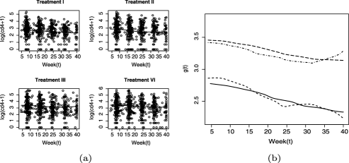
Figure 1: (a) The raw data excluding missing values plots with the estimates of $g_{j}(t)$ ($j=1,2,3,4$). (b) The estimates of $g_{j}(t)$ in the same plot: treatment I (solid line), treatment II (short dashed line), treatment III (dashed and doted line) and treatment IV (long dashed line).

We then tested for the nonparametric baseline time effects. The kernel estimates $\hat{g}_{j}(t)$ are displayed in Figure 1, which shows that treatments I and II and treatments III and IV had similar baselines evolution overtime, respectively. However, a big difference existed between the first two treatments and the last two treatments. Treatment IV decreased more slowly than that of the other three treatments, which seemed to be the most effective in slowing down the decline of CD4. We also found that during the first 16 weeks the CD4 counts decrease slowly and then the decline became faster after 16 weeks for treatments I, II and III.

The $p$-value for testing $H_{0b}\dvtx g_{1}(\cdot)=g_{2}(\cdot)=g_{3}(\cdot)=g_{4}(\cdot)$ is shown in Table 9. The entries were based on 500 bootstrapped resamples according to the procedure introduced in Section 6. The statistics ${\mathcal{T}}_{n}$ for testing $H_{0b}\dvtx g_{1}(\cdot)=g_{2}(\cdot)=g_{3}(\cdot)=g_{4}(\cdot)$ was 3965.00, where we take $\varpi(t)=1$ over the range of $t$. The $p$-value of the test was 0.004. Thus, there existed significant difference in the baseline time effects $g_{j}(\cdot)$’s among treatments I–IV. At the same time, we also calculate the test statistics ${\mathcal{T}}_{n}$ for testing $g_{1}(\cdot)=g_{2}(\cdot)$ and $g_{3}(\cdot)=g_{4}(\cdot)$. The statistics values were 19.26 and 26.22, with $p$-values 0.894 and 0.860, respectively. These $p$-values are much bigger than 0.05. We conclude that treatment I and II has similar baseline time effects, but they are significantly distinct from the baseline time effects of treatment III and IV, respectively. $p$-values of testing other combinations on equalities of $g_{1}(\cdot),g_{2}(\cdot),g_{3}(\cdot)$ and $g_{4}(\cdot)$ are also reported in Table 9.

Table 9: $p$-values of ANOVA tests on $g_{j}(\cdot)$’s

$\bolds{H_{0b}}$	$\bolds{p}$-value	$\bolds{H_{0b}}$	$\bolds{p}$-value
$g_{1}(\cdot)=g_{2}(\cdot)$	0.894	$g_{1}(\cdot)=g_{2}(\cdot)=g_{3}(\cdot)$	0.046
$g_{1}(\cdot)=g_{3}(\cdot)$	0.018	$g_{1}(\cdot)=g_{2}(\cdot)=g_{4}(\cdot)$	0.010
$g_{1}(\cdot)=g_{4}(\cdot)$	0.004	$g_{1}(\cdot)=g_{3}(\cdot)=g_{4}(\cdot)$	0.000
$g_{2}(\cdot)=g_{3}(\cdot)$	0.020	$g_{2}(\cdot)=g_{3}(\cdot)=g_{4}(\cdot)$	0.014
$g_{2}(\cdot)=g_{4}(\cdot)$	0.006	$g_{1}(\cdot)=g_{2}(\cdot)=g_{3}(\cdot)=g_{4}(\cdot)$	0.004
$g_{3}(\cdot)=g_{4}(\cdot)$	0.860

This data set has been analyzed by Fitzmaurice, Laird and Ware (2004) using a random effects model that applied the Restricted Maximum Likelihood (REML) method. They conducted a two sample comparison test via parameters in the model for the difference between the dual therapy (treatment I–III) versus triple therapy (treatment VI) without considering the missing values. More specifically, they denoted $\mathrm{Group}=1$ if subject in the triple therapy treatment and $\mathrm{Group}=0$ if subject in the dual therapy treatment, and the linear mixed effect was

$$E(Y|b) = \beta_{1}+\beta_{2}t+\beta_{3}(t-16)_{+}+{\beta_{4}\operatorname{Group}}\times t$$

$${}+{\beta_{5}\operatorname{Group}}\times(t-16)_{+}+b_{1}+b_{2}t+b_{3}(t-16)_{+},$$

where $b=(b_{1},b_{2},b_{3})$ are random effects. They tested $H_{0}\dvtx\beta_{4}=\beta_{5}=0$. This is equivalent to test the null hypothesis of no treatment group difference in the changes in $\log$ CD4 counts between therapy and dual treatments. Both Wald test and likelihood ratio test rejected the null hypothesis, indicating the difference between dual and triple therapy in the change of $\log$ CD4 counts. Their results are consistent with the result we illustrated in Table 9.

Appendix: Technical assumptions

We provides the conditions used for Theorems 1–5 and some remark in this section. The proofs for Theorems 1, 2, 3 and 5 are contained in the supplement article [Chen and Zhong (2010)]. The proof for Theorem 4 is largely similar to that of Theorem 1 and is omitted.

The following assumptions are made in the paper:

1. [A1.]

2. Let $S(\theta_{j})$ be the score function of the partial likelihood ${\mathcal{L}}_{B_{j}}(\theta_{j})$ for a q-dimensional parameter $\theta_{j}$ defined in (2), and $\theta_{j0}$ is in the interior of compact $\Theta_{j}$. We assume $E\{S(\theta_{j})\}\neq 0$ if $\theta_{j}\neq\theta_{j0}$, $\operatorname{Var}(S(\theta_{j0}))$ is finite and positive definite, and $E(\frac{\partial S(\theta_{j0})}{\partial\theta_{j0}})$ exists and is invertible. The missing propensity $\pi_{jim}(\theta_{j0})>b_{0}>0$ for all $j,i,m$.

3. 1. [(iii)]

   2. The kernel function $K$ is a symmetric probability density which is differentiable of Lipschitz order 1 on its support $[-1,1]$. The bandwidths satisfy $n_{j}h_{j}^{2}/\log^{2}n_{j}\rightarrow\infty$, $n_{j}^{1/2}h_{j}^{4}\rightarrow 0$ and $h_{j}\rightarrow 0$ as $n_{j}\rightarrow\infty$.

   3. For each treatment $j$ $(j=1,\ldots,k)$, the design points $\{t_{jim}\}$ are thought to be independent and identically distributed from a super-population with density $f_{j}(t)$. There exist constants $b_{l}$ and $b_{u}$ such that $0<b_{l}\leq\sup_{t\in S}f_{j}(t)\leq b_{u}<\infty$.

   4. For each $h_{j}$ and $T_{j}$, $j=1,\ldots,k$, there exist finite positive constants $\alpha_{j}$, $b_{j}$ and $T$ such that $\alpha_{j}T_{j}=T$ and $b_{j}h_{j}=h$ for some $h$ as $h\to 0$. Let $n=\sum_{i=1}^{k}n_{j},n_{j}/n\rightarrow\rho_{j}$ for some nonzero $\rho_{j}$ as $n\rightarrow\infty$ such that $\sum_{i=1}^{k}\rho_{j}=1$.

4. The residuals $\{\varepsilon_{ji}\}$ and $\{u_{ji}\}$ are independent of each other and each of $\{\varepsilon_{ji}\}$ and $\{u_{ji}\}$ are mutually independent among different $j$ or $i$,respectively; $\max_{1\leq i\leq n_{j}}\|u_{jim}\|=o_{p}\{n_{j}^{({2+r})/({2(4+r)})}(\log n_{j})^{-1}\}$,$\max_{1\leq i\leq n_{j}}E|\varepsilon_{jim}|^{4+r}<\infty$, for some $r>0$; and assume that

   $$\lim_{n_{j}\rightarrow\infty}(n_{j}T_{j})^{-1}\sum_{i=1}^{n_{j}}\sum_{m=1}^{T_{j}}E\{\widetilde{\mathbb{X}}_{jim}\widetilde{\mathbb{X}}_{jim}^{\tau}\}=\Sigma_{x}>0,$$

   where $\widetilde{\mathbb{X}}_{jim}=\mathbb{X}_{jim}-E(\mathbb{X}_{jim}|t_{jim})$.

5. The functions $g_{j0}(t)$ and $h_{j}(t)$ are, respectively, one-dimensional and $p$-dimensional smooth functions with continuously second derivatives on $S=[0,1]$.

Condition A1 are the regular conditions for the consistency of the binary MLE for the parameters in the missing propensity. Condition A2(i) are the usual conditions for the kernel and bandwidths in nonparametric curve estimation. Note that the optimal rate for the bandwidth $h_{j}=O(n_{j}^{-1/5})$ satisfies A2(i). The requirement of design points $\{t_{jim}\}$ in A2(ii) is a common assumption similar to the ones in Müller (1987). Condition A2(iii) is a mild assumption on the relationship between bandwidths and sample sizes among different samples. In A3, we do not require the residuals $\{\varepsilon_{ji}\}$ and $\{u_{ji}\}$ being, respectively, identically distributed for each fixed $j$. This allows extra heterogeneity among individuals for a treatment. The positive definite of $\Sigma_{x}$ in condition A3 is used to identify the “parameters” $(\beta_{j0},\gamma_{j0},g_{j0})$ uniquely, which is a generalization of the identification condition used in Härdle, Liang and Gao (2000) to longitudinal data. This condition can be checked empirically by constructing consistent estimate of $\Sigma_{x}$.

References

• Cao and Van Keilegom (2006) Cao, R. and Van Keilegom, I. (2006). Empirical likelihood tests for two-sample problems via nonparametric density estimation. Canad. J. Statist. 34 61–77. \MR2267710
• Chen and Cui (2006) Chen, S. X. and Cui, H.-J. (2006). On Bartlett correction of empirical likelihood in the presence of nuisance parameters. Biometrika 93 215–220. \MR2277752
• Chen and Hall (1994) Chen, S. X. and Hall, P. (1994). On the calculation of standard error for quotation in confidence statements. Statist. Probab. Lett. 19 147–151.
• Chen, Leung and Qin (2008) Chen, S. X., Leung, D. and Qin, J. (2008). Improved semiparametric estimation using surrogate data. J. R. Stat. Soc. Ser. B Stat. Methodol. 70 803–823. \MR2523905
• Chen and Van Keilegom (2009) Chen, S. X. and Van Keilegom, I. (2009). A review on empirical likelihood for regressions. TEST 18 415–447. \MR2566404
• Chen and Zhong (2010) Chen, S. X. and Zhong, P.-S. (2010). A Supplement to “ANOVA for longitudinal data with missing values.” DOI: 10.1214/10-AOS824SUPP.
• DiCicco, Hall and Romano (1991) DiCicco, T., Hall, P. and Romano, J. (1991). Empirical likelihood is Barterlett-correctable. Ann. Statist. 19 1053–1061. \MR1105861
• Fan, Huang and Li (2007) Fan, J., Huang, T. and Li, R. (2007). Analysis of longitudinal data with semiparametric estimation of covariance function. J. Amer. Statist. Assoc. 102 632–641. \MR2370857
• Fan and Zhang (2004) Fan, J. and Zhang, J. (2004). Sieve empirical likelihood ratio tests for nonparametric functions. Ann. Statist. 32 1858–1907. \MR2102496
• Fitzmaurice, Laird and Ware (2004) Fitzmaurice, G., Laird, N. and Ware, J. (2004). Applied Longitudinal Analysis. Wiley, Hoboken, NJ. \MR2063401
• Forcina (1992) Forcina, A. (1992). Modelling balanced longitudinal data: Maximum likelihood estimation and analysis of variance. Biometrics 48 743–750. \MR1187599
• Härdle, Liang and Gao (2000) Härdle, W., Liang, H. and Gao, J. (2000). Partially Linear Models. Physica-Verlag, Heidelberg.
• Härdle and Mammen (1993) Härdle, W. and Mammen, E. (1993). Comparing nonparametric versus parametric regression fits. Ann. Statist. 21 1926–1947. \MR1245774
• Henry et al. (1998) Henry, K., Erice, A., Tierney, C., Balfour, H., Fischl, M., Kmack, A., Liou, S., Kenton, A., Hirsch, M., Phair, J., Martinez, A. and Kahn, J. for the AIDS Clinical Trial Group 193A Study Team (1998). A randomized, controlled, double-blind study comparing the survival benefit of four different reverse transcriptase inhibitor therapies (three-drug, two-drug, and alternating drug) for the treatment of advanced AIDS. Journal of Acquired Immune Deficiency Syndromes And Human Retrovirology 19 339–349.
• Huang, Qin and Follmann (2008) Huang, C. Y., Qin, J. and Follmann, D. (2008). Empirical likelihood-based estimation of the treatment effect in a pretest-posttest study. J. Amer. Statist. Assoc. 103 1270–1280. \MR2462898
• Laird (2004) Laird, N. (2004). Analysis of Longitudinal and Cluster-Correlated Data. IMS, Beachwood, OH.
• Laird and Ware (1982) Laird, N. and Ware, J. (1982). Random-effects models for longitudinal data. Biometrics 38 963–974.
• Liang and Qin (2008) Liang, H. and Qin, Y.-S. (2008). Empirical likelihood-based inferences for partially linear models with missing covariates. Aust. N. Z. J. Stat. 50 347–359. \MR2474196
• Liang and Zeger (1986) Liang, K. and Zeger, S. (1986). Longitudinal data analysis using generalized linear models. Biometrica 73 13–22. \MR0836430
• Lin and Ying (2001) Lin, D. and Ying, Z. (2001). Semiparametric and nonparametric regression analysis of longitudinal data. J. Amer. Statist. Assoc. 96 103–126. \MR1952726
• Linton and Nielsen (1995) Linton, O. and Nielsen J. (1995). A kernel method of estimating structured nonparametric regression based on marginal integration. Biometrika 82 93–100. \MR1332841
• Liu (1988) Liu, R. (1988). Bootstrap procedures under some non-i.i.d. models. Ann. Statist. 16 1696–1708. \MR0964947
• Little and Rubin (2002) Little, R. and Rubin, B. (2002). Statistical Analysis with Missing Data, 2nd ed. Wiley, Hoboken, NJ. \MR1925014
• Little (1995) Little, R. (1995). Modeling the drop-out mechanism in repeated-measures studies. J. Amer. Statist. Assoc. 90 1112–1121. \MR1354029
• Müller (1987) Müller, H. (1987). Weighted local regression and kernel methods for nonparametric curve fitting. J. Amer. Statist. Assoc. 82 231–238. \MR0883351
• Mund and Dettle (1998) Mund, A. and Dettle, H. (1998). Nonparametric comparison of several regression functions: Exact and asymptotic theory. Ann. Statist. 26 2339–2368. \MR1700235
• Owen (1988) Owen, A. (1988). Empirical likelihood ratio confidence intervals for a single functional. Biometrika 75 237–249. \MR0946049
• Owen (1990) Owen, A. (1990). Empirical likelihood ratio confidence regions. Ann. Statist. 18 90–120. \MR1041387
• Owen (2001) Owen, A. (2001). Empirical Likelihood. Chapman and Hall/CRC, Boca Raton, FL.
• Pardo-Fernández, Van Keilegom and González-Manteiga (2007) Pardo-Fernández, J., Van Keilegom, I. and González-Manteiga, W. (2007). Testing for the equality of $k$ regression curves. Statist. Sinica 17 1115–1137. \MR2397389
• Qin and Lawless (1994) Qin, J. and Lawless, J. (1994). Empirical likelihood and general estimating equations. Ann. Statist. 22 300–325. \MR1272085
• Rice and Silverman (1991) Rice, J. and Silverman, B. (1991). Estimating the mean and covariance structure nonparametrically when the data are curves. J. Roy. Statist. Soc. Ser. B 53 233–243. \MR1094283
• Robins, Rotnitzky and Zhao (1995) Robins, J., Rotnitzky, A. and Zhao, L. (1995). Analysis of semiparametric regression models for repeated outcomes in the presence of missing data. J. Amer. Statist. Assoc. 90 106–121. \MR1325118
• Rubin (1976) Rubin, B. (1976). Inference and missing data (with discussion). Biometrika 63 581–592. \MR0455196
• Scheike and Zhang (1998) Scheike, T. H. and Zhang, M. J. (1998). Cumulative regression function tests for regression models for longitudinal data. Ann. Statist. 26 1328–1355. \MR1647665
• Shao and Sitter (1996) Shao, J. and Sitter, R. (1996). Bootstrap for imputed survey data. J. Amer. Statist. Assoc. 91 1278–1288. \MR1424624
• Speckman (1988) Speckman, P. (1988). Kernel smoothing in partial linear models. J. Roy. Statist. Soc. Ser. B 50 413–436. \MR0970977
• Wang, Akritas and Van Keilegom (2008) Wang, L., Akritas, M. and Van Keilegom, I. (2008). An ANOVA-type nonparametric diagnostic test for heteroscedastic regression models. J. Nonparametr. Stat. 20 365–382. \MR2424247
• Wang, Carroll and Lin (2005) Wang, N., Carroll, R. and Lin, X. (2005). Efficient marginal estimation for longitudinal/clustered data. J. Amer. Statist. Assoc. 100 147–157. \MR2156825
• Wang, Linton and Härdle (2004) Wang, Q.-H., Linton, O. and Härdle, W. (2004). Semiparametric regression analysis with missing response at random. J. Amer. Statist. Assoc. 99 334–345. \MR2062820
• Wang and Rao (2002) Wang, Q.-H. and Rao, J. (2002). Empirical likelihood-based inference under imputation for missing response data. Ann. Statist. 30 896–924. \MR1922545
• Wu (1986) Wu, C.-F.-J. (1986). Jackknife, bootstrap and other resampling method in regression analysis. Ann. Statist. 14 1261–1295. \MR0868303
• Wu, Chiang and Hoover (1998) Wu, C., Chiang, C. and Hoover, D. (1998). Asymptotic confidence regions for kernel smoothing of a varying-coefficient model with longitudinal data. J. Amer. Statist. Assoc. 93 1388–1402. \MR1666635
• Wu and Chiang (2000) Wu, C. and Chiang, C. (2000). Kernel smoothing on varying coefficient models with longitudinal dependent variable. Statist. Sinica 10 433–456. \MR1769751
• Xue and Zhu (2007a) Xue, L. and Zhu, L. (2007a). Empirical likelihood semiparametric regression analysis for longitudinal data. Biometrika 94 921–937. \MR2416799
• Xue and Zhu (2007b) Xue, L. and Zhu, L. (2007b). Empirical likelihood for a varying voefficient model with longitudinal data. J. Amer. Statist. Assoc. 102 642–654. \MR2370858
• You, Chen and Zhou (2006) You, J., Chen, G. and Zhou, Y. (2006). Block empirical likelihood for longitudinal partially linear regression models. Canad. J. Statist. 34 79–96. \MR2267711
• Zeger and Diggle (1994) Zeger, S. and Diggle, P. (1994). Semiparametric models for longitudinal data with application to CD4 cell numbers in HIV seroconverters. Biometrics 50 689–699.
• Zhang et al. (1998) Zhang, D., Lin, X., Raz, J. and Sowers, J. (1998). Semiparametric stochastic mixed models for longitudinal data. J. Amer. Statist. Assoc. 93 710–719. \MR1631369