RKKY interaction in carbon nanotubes and graphene nanoribbons

Abstract

We study Rudermann-Kittel-Kasuya-Yosida (RKKY) interaction in carbon nanotubes (CNTs) and graphene nanoribbons in the presence of spin orbit interactions and magnetic fields. For this we evaluate the static spin susceptibility tensor in real space in various regimes at zero temperature. In metallic CNTs the RKKY interaction depends strongly on the sublattice and, at the Dirac point, is purely ferromagnetic (antiferromagnetic) for the localized spins on the same (different) sublattice, whereas in semiconducting CNTs the spin susceptibility depends only weakly on the sublattice and is dominantly ferromagnetic. The spin orbit interactions break the SU(2) spin symmetry of the system, leading to an anisotropic RKKY interaction of Ising and Moryia-Dzyaloshinsky form, besides the usual isotropic Heisenberg interaction. All these RKKY terms can be made of comparable magnitude by tuning the Fermi level close to the gap induced by the spin orbit interaction. We further calculate the spin susceptibility also at finite frequencies and thereby obtain the spin noise in real space via the fluctuation-dissipation theorem.

I Introduction

The Rudermann-Kittel-Kasuya-Yosida (RKKY) interaction is an indirect exchange interaction between two localized spins induced by itinerant electrons in a host material.Ruderman_1954 ; Kasuya_1956 ; Yosida_1957 This effective spin interaction, being determined by the static spin susceptibility, is not only a fundamental characteristics of the host system but also finds interesting and useful applications. One of them is the long-range coupling of spins between distant quantum dots, Craig_2004 ; Rikitake_2005 which is needed in scalable quantum computing architectures such as the surface code Wang_2011 built from spin qubits. Trifunovic_2012 In addition, the RKKY interaction, enhanced by electron-electron interactions, can initiate a nuclear spin ordering that leads to striking effects such as helical nuclear magnetism at low temperatures. Braunecker_2009_PRL ; Braunecker_2009_PRB Such a rotating magnetic field, equivalent to the presence of a uniform magnetic field and Rashba spin orbit interaction (SOI) in one-dimensional systems,Braunecker_Jap_Klin_2009 is interesting for Majorana fermion physics in its own right. Braunecker_Jap_Klin_2009 ; Flensberg_Rot_Field ; Two_field_Klinovaja ; klinovaja_Nanoribbon The RKKY interaction, proposed long ago for normal metals of Fermi liquid type,Ruderman_1954 ; Kasuya_1956 ; Yosida_1957 ; giuliani_book was later extended in various ways, in particular to low-dimensional systems with Rashba SOI in the clean Bruno_2004 and the disordered stefano_2010 limit, and to systems with electron-electron interactions in one Egger_1996 ; Braunecker_2009_PRL ; Braunecker_2009_PRB and two dimensions with zak_2012 and without RKKY_2D ; Chesi_2008 Rashba SOI. Also, a general theorem of Mermin-Wagner type was recently proven for isotropic RKKY systems that excludes magnetic ordering in one and two dimensions at any finite temperature but allows it in the presence of SOI. order_2_2011 ; Governale_2012

Moreover, due to recent progress in magnetic nanoscale imaging,amir one can expect that the direct measurement of the static spin susceptibility has become within experimental reach.stm_2010 For this latter purpose, graphene offers the unique advantage over other materials such as GaAs heterostructures in that its surface can be accessed directly on a atomistic scale by the sensing device. All this makes the spin susceptibility and the RKKY interaction important quantities to study.

Recently, the RKKY interaction in graphene has attracted considerable attention.Vozmediano_2005 ; Dugaev_2006 ; saremi_2007 ; Black_2010 ; kogan_2011 ; Sherafati_2011 Graphene is known for its Dirac-like spectrum with a linear dispersion at low energies. This linearity, however, can give rise to divergences in the expression for the spin susceptibility in momentum space saremi_2007 and complicates the analysis compared to systems with quadratic dispersion. However, Kogan recently showed that these divergences can be avoided by working in the Matsubara formalism. kogan_2011

In the present work we consider the close relatives of graphene,dresselhaus_book namely carbon nanotubes (CNTs) and graphene nanoribbons (GNRs), with a focus on spin orbit interaction and non-uniform magnetic fields. Metallic CNTs also have a linear spectrum, so for them the imaginary time approach developed in Ref. kogan_2011, is also most convenient and will be used here. Analogously to graphene, we find that the static spin susceptibility changes sign, depending on whether the localized spins belong to the same sublattice or to different sublattices. footnote_1 No such dependence occurs for CNTs in the semiconducting regime, characterized by a gap and parabolic spectrum at low fillings.

The spin orbit interaction in CNTs is strongly enhanced by curvature effects in comparison to flat graphene, izumida ; cnt_helical_2011 ; klinovaja_cnt while in GNRs strong SOI-like effects can be generated by magnetic fields that oscillate or rotate in real space. Two_field_Klinovaja ; klinovaja_Nanoribbon Such non-uniform fields can be produced for instance by periodically arranged nanomagnets. exp_field Spin orbit effects break the SU(2) spin-symmetry of the itinerant carriers and thus lead, besides the effective Heisenberg interaction, to anisotropic RKKY terms of Moryia-Dzyaloshinsky and of Ising form. Quite remarkably, when the Fermi level is tuned close to the gap opened by the SOI, we find that the isotropic and anisotropic terms become of comparable size. This has far reaching consequences for ordering in Kondo lattices with RKKY interaction, since this opens up the possibility to have magnetic phase transitions in low-dimensional systems at finite temperature that are tunable by electric gates.

We mention that similar anisotropies have been found before for semiconductors with parabolic spectrum and with Rashba SOI in the clean Bruno_2004 and in the disordered stefano_2010 limit. However, the spin orbit interactions in CNTs and in GNRs are of different symmetry and thus both of these problems require a separate study, apart from the fact that the spectrum is linear.

For all itinerant regimes we consider, the RKKY interaction is found to decay as $1/R$, where $R$ is the distance between the localized spins, thus following the standard behavior for RKKY interaction in non-interacting one-dimensional systems. giuliani_book [In interacting systems, described by Luttinger liquids, the decay becomes slower. Egger_1996 ; Braunecker_2009_PRB ; Imambekov_RMF ] In contrast, the overall sign as well as the spatial oscillation periods of the RKKY interaction are non-generic and depend strongly on the system and the regimes considered.

Finally, we will also consider the dynamical spin susceptibility at finite frequency. Via the fluctuation-dissipation theorem we obtain from this the spin-dependent dynamical structure factor in position space, which describes the equilibrium correlations of two localized spins separated by a distance $R$.

The paper is organized as follows. Sec. II contains different approaches to the RKKY interaction including imaginary time formalism for metallic CNTs with a linear spectrum and the retarded Green functions in the real space formalism for semiconducting CNTs. In Sec. III the low energy spectrum of CNTs is shortly discussed. Afterwards the spin susceptibility is calculated both in the absence of the SOI (Sec. IV) and in the presence of the SOI (Sec. V). In addition, in Sec. VI we present results for the case of a magnetic field along the nanotube axis. Such a field breaks both orbital and spin degeneracy, leading to non-trivial dependence of the spin susceptibility on the chemical potential. The fluctuation-dissipation theorem connects the spin susceptibility and the spin fluctuations, allowing us to explore the frequency dependence of the spin noise at zero temperature in Sec. VII. The RKKY interaction in armchair graphene nanoribbons is briefly considered in Sec. VIII. Finally, we conclude with Sec. IX in which we shortly summarize our main results.

II Formalism for RKKY

The RKKY interactionRuderman_1954 ; Kasuya_1956 ; Yosida_1957 was studied for a long time and several approaches were developed. In this section we briefly review those used in this work.

The RKKY interaction is an effective exchange interaction between two magnetic spins, $\mathbf{I}_{i}$ and $\mathbf{I}_{j}$, localized at lattice sites $\mathbf{R}_{i}$ and $\mathbf{R}_{j}$, respectively, that are embedded in a system of itinerant electrons with spin-1/2. These electrons have a local spin-interaction with the localized spins, described by the Hamiltonian

$$H_{int}=J\sum_{l=i,j}\mathbf{s}_{l}\cdot\mathbf{I}_{l},$$ (1)

where $\hbar\mathbf{s}_{l}/2$ is the electron spin operator at site $\mathbf{R}_{l}$, and $J$ is the coupling strength. Using second order perturbation expansion in $J$, giuliani_book ; Bruno_2004 ; Braunecker_2009_PRB ; kogan_2011 the RKKY Hamiltonian Ruderman_1954 ; Kasuya_1956 ; Yosida_1957 becomes

$$H_{RKKY}=J^{2}\chi^{ij}_{\alpha\beta}I^{\alpha}_{i}I^{\beta}_{j},$$ (2)

where $\chi^{ij}_{\alpha\beta}=\chi_{\alpha\beta}(\mathbf{R}_{ij},\omega=0)$ is the static (zero-frequency) spin susceptibility tensor, and where summation is implied over repeated spin indices $\alpha,\beta=x,y,z$ (but not over $i,j$). Here, we assumed that the system is translationally invariant so that the susceptibility depends only on the relative distance $\mathbf{R}_{ij}\equiv\mathbf{R}_{i}-\mathbf{R}_{j}$. The RKKY interaction can be expressed in several equivalent ways. For example, in terms of the retarded Green function $G(\mathbf{R}_{ij};\epsilon+i0^{+})$ the RKKY Hamiltonian is given by

$$H_{RKKY}=-\frac{J^{2}}{\pi}{\rm Im}\int_{-\infty}^{\epsilon_{F}}d\epsilon\ {\rm Tr}\left[(\mathbf{I}_{i}\cdot\mathbf{s})(\mathbf{I}_{j}\cdot\mathbf{s})\right.$$

$$\ \ \ \ \ \ \ \ \ \ \ \ \ \ \ \ \left.\times G(\mathbf{R}_{ij};\epsilon+i0^{+})G(-\mathbf{R}_{ij};\epsilon+i0^{+})\right],$$ (3)

where the integration over energy $\epsilon$ is limited by the Fermi energy $\epsilon_{F}$ (see Ref. Bruno_2004, ). Here $\mathbf{s}$ is a vector of the Pauli matrices acting on the spin of the itinerant electrons, and the trace Tr runs over the electron spin. The retarded Green function $G(\mathbf{R}_{ij};\epsilon+i0^{+})$, which are spin-dependent here and represented as $2\times 2$-matrices in spin space, are taken in real ($\mathbf{R}_{ij}$) and energy space ($\epsilon$). In the presence of spin orbit interaction, we will use Eq. (3) as a starting point.

In the absence of spin orbit interaction, the spin is a good quantum number, so the effective Hamiltonian $H_{RKKY}$ can be significantly simplified, $\chi^{ij}_{\alpha\beta}=\delta_{\alpha\beta}\chi^{ij}_{0}$, and the RKKY interaction is of Heisenberg type (isotropic in spin space). Expressing the Green functions in terms of the eigenfunctions $\psi_{n}(\mathbf{R}_{i})$ of the electron Hamiltonian, we obtain

$$\chi^{ij}_{0}=2\sum_{n,m}\psi_{n}^{*}(\mathbf{R}_{i})\psi_{m}(\mathbf{R}_{i}) \psi_{n}(\mathbf{R}_{j})\psi_{m}^{*}(\mathbf{R}_{j})$$

$$\times\frac{n_{F}(\xi_{n})-n_{F}(\xi_{m})}{\xi_{n}-\xi_{m}},$$ (4)

where the sum runs over all eigenstates of the spinless system, and the factor $2$ accounts for the spin degeneracy. The energy is calculated from the Fermi level, $\xi_{n}=\epsilon_{n}-\epsilon_{F}$, and the Fermi distribution function at $T=0$ is given by $n_{F}(\xi)=\theta(-\xi)$.

The sum in Eq. (4) is divergent in case of a linear spectrum.yafet_1987 ; kogan_2011 To avoid these divergences we follow Ref. kogan_2011, and work in the imaginary time formalism, again neglecting the spin structure of the Green functions. The static real space spin susceptibility at zero temperature is given by

$$\chi^{ij}_{0}=\frac{2}{\hbar}\int_{0}^{\infty}d\tau\ G_{0}(\mathbf{R}_{ij},\tau)G_{0}(-\mathbf{R}_{ij},-\tau),$$ (5)

where the factor 2 again accounts for the spin degeneracy. The Matsubara Green functions for $\tau\geq 0$ are found as

$$G_{0}(\mathbf{R}_{ij},\pm\tau)=\mp\sum_{n} \psi_{n}^{*}(\mathbf{R}_{i})\psi_{n}(\mathbf{R}_{j})e^{\mp\xi_{n}\tau/\hbar}\theta(\pm\xi_{n}).$$ (6)

All three approaches to the RKKY interaction described above [see Eqs. (3), (4), and (5)] are equivalent to each other. Which one is used for a particular case depends on calculational convenience.

III Carbon nanotubes

In this section, we discuss the effective Hamiltonian for a carbon nanotube. A carbon nanotube is a rolled-up sheet of graphene, a honeycomb lattice composed of two types of non-equivalent atoms $A$ and $B$. The $(N_{1},N_{2})$-CNTs can be alternatively characterized by the chiral angle $\theta$ and the diameter $d$.dresselhaus_book The low-energy physics takes place in two valleys $\bf K$ and $\bf K^{\prime}$. These two Dirac points are determined by $\mathbf{K}=-\mathbf{K}^{\prime}=4\pi({\bf\hat{t}}\cos\theta+{\bf\hat{z}}\sin\theta)/3a$, where $a$ is the lattice constant. The unit vector ${\bf\hat{z}}$ points along the CNT axis, and ${\bf\hat{t}}$ is the unit vector in the transverse direction.

III.1 Effective Hamiltonian

In the absence of spin orbit interaction CNTs are described by the effective Hamiltonian $H_{0}$,

$$H_{0}=\hbar v_{F}(k_{G}\sigma_{1}+k\gamma\sigma_{2}).$$ (7)

The Pauli matrices $\sigma_{i}$ act in the space defined by the sublattices $A$ and $B$. The Fermi velocity in graphene $\upsilon_{F}$ is equal to $10^{6}\ \rm{m/s}$. Here, $\gamma=1\ (\gamma=-1)$ labels the $\mathbf{K}$ ($\mathbf{K}^{\prime}$) Dirac points, and $k$ is the momentum along the $z$-axis calculated from the corresponding Dirac point. The momentum in the circumferential direction $k_{G}$ is quantized, $k_{G}=2(m-\gamma\delta/3)/d$, with $d$ the CNT diameter, leading to two kinds of nanotubes: metallic and semiconducting. Here, $m\in\mathbb{Z}$ is the subband index and $\delta=(N_{1}-N_{2})\ {\rm mod}\,3$ for a $(N_{1},N_{2})$-CNT (see Ref. dresselhaus_book, ). The spectrum of metallic CNTs (with $k_{G}=0$) is a Dirac cone, i.e. linear and gapless. In contrast to that, the spectrum of semiconducting CNTs (with $k_{G}\neq 0$) has a gap given by $2\hbar v_{F}|k_{G}|$. In the following we consider only the lowest subband with energies

$$\epsilon_{n}=\nu\hbar v_{F}\sqrt{k^{2}+k_{G}^{2}},$$ (8)

where $\nu=1$ ($\nu=-1$) corresponds to electrons (holes), and $n=(k,\gamma,\nu)$ labels the eigenstates. The corresponding wavefunctions with sublattice spinor are given by

$$\psi_{n}(\mathbf{R}_{i})=e^{i(\gamma\mathbf{K}+\mathbf{k})\cdot\mathbf{R}_{i}}\frac{1}{\sqrt{2}}\begin{pmatrix}1\\ \nu\gamma e^{i\phi_{k}}\end{pmatrix},$$ (9)

$$e^{i\phi_{k}}=\frac{k_{G}+ik}{\sqrt{k_{G}^{2}+k^{2}}},$$ (10)

where $\mathbf{k}=(k_{G},k)$. From now on we redefine Dirac points by shifting the circumferential value of $\mathbf{K}$ ($\mathbf{K}^{\prime}$) by $k_{G}$, so that $\mathbf{K}=-\mathbf{K}^{\prime}=4\pi({\bf\hat{t}}\cos\theta+{\bf\hat{z}}\sin\theta)/3a+{\bf\hat{t}}k_{G}$ and $\mathbf{k}=(0,k)$.

III.2 Spin orbit interaction

Spin orbit interaction in nanotubes arises mostly from curvature effects, which substantially increase its value in comparison with flat graphene. izumida ; cnt_helical_2011 ; klinovaja_cnt ; cnt_ext_kuemmeth ; cnt_ext_kop ; cnt_ext_delft The effective Hamiltonian, which includes the spin orbit interaction terms, is given by

$$H_{so}=H_{0}+\alpha\sigma_{1}s_{z}+\gamma\beta s_{z},$$ (11)

where $s_{i}$ are the Pauli matrices acting on the spin. The SOI is described by two parameters, $\alpha$ and $\beta$, which depend on the diameter $d$. The values of these parameters can be found in the framework of the tight-binding model, $\alpha=-0.16\ {\rm meV}/d\ {\rm[nm]}$ and $\beta=-0.62\ {\rm meV}\cos(3\theta)/d\ {\rm[nm]}$ (see Refs. cnt_helical_2011, ; klinovaja_cnt, ). The valley index $\gamma$ and the spin projection on the nanotube axis $s$ are good quantum numbers due to the rotation invariance of the CNT. The conduction band spectrum ($\nu=1$) is given by

$$\epsilon_{n}=\pm\gamma\beta s+\sqrt{(\hbar\upsilon_{F}k)^{2}+(\gamma\hbar\upsilon_{F}k_{G}+\alpha s)^{2}}\,,$$ (12)

and the corresponding wavefunctions are given by

$$\psi_{n}(\mathbf{R}_{i})=e^{i(\gamma\mathbf{K}+\mathbf{k})\cdot\mathbf{R}_{i}}\frac{1}{\sqrt{2}}\begin{pmatrix}1\\ e^{i\phi_{s,\gamma}}\end{pmatrix}\left|s\right\rangle,$$ (13)

$$e^{i\phi_{s,\gamma}}=\frac{\gamma k_{G}+s\alpha+i\gamma k}{\sqrt{k^{2}+(\gamma k_{G}+s\alpha)^{2}}},$$ (14)

where the index $n=(k,\gamma,s)$ labels the eigenstates. Here $\left|s\right\rangle$, the eigenstate of the Pauli matrix $s_{z}$, corresponds to the spin state with spin up ($s=1$) or down ($s=-1$). We note that the SOI lifts the spin degeneracy and opens gaps at zero momentum, $k=0$. In case of semiconducting nanotubes ($k_{G}\gg k$), we use the parabolic approximation of the spectrum,

$$\epsilon_{n}=\hbar\upsilon_{F}k_{G}+\gamma s(\beta+\alpha)+\hbar\upsilon_{F}k^{2}/2k_{G}.$$ (15)

Further we denote the sum of the SOI parameters $\alpha$ and $\beta$ as $\beta_{+}\equiv\beta+\alpha$. Such kind of a spectrum is similar to the spectrum of a CNT in the presence of a pseudo-magnetic field that has opposite signs at opposite valleys. We note that there is a principal difference between a semiconducting CNT and a semiconducting nanowire with Rashba SOI. In the latter, the Rashba SOI can be gauged away by a spin-dependent unitary transformation.Bruno_2004 ; Braunecker_Jap_Klin_2009 In contrast, the spectrum of CNTs consists of parabolas shifted along the energy axis and not along the momentum axis as in the case of semiconducting nanowires, so the SOI cannot be gauged away. As shown below, this leads to a less transparent dependence of the spin susceptibility on the SOI compared to nanowires. Bruno_2004

IV RKKY in the absence of SOI

In this section we calculate the spin susceptibility neglecting spin orbit interaction, so all states are two-fold degenerate in spin. We can thus consider a spinless system and account for the spin degeneracy just by introducing a factor of 2 in the expressions for the spin susceptibility, see Eqs. (4) and (5).

IV.1 Metallic nanotubes

The spectrum of a metallic nanotube is linear, see Eq. (8), with the momentum in the circumferential direction $k_{G}$ equal to zero, $k_{G}=0$. As was mentioned above, in this case the integrals over the momentum in Eq. (4) are divergent, kogan_2011 so it is more convenient to work in the imaginary time formalism [see Eq. (5)], where all integrals remain well-behaved. To simplify notations, we denote the distance between the localized spins as $\mathbf{R}\equiv\mathbf{R}_{i}-\mathbf{R}_{j}$ and its projection on the CNT axis as $z$. Using the wavefunctions given by Eq. (9), we find the Green functions from Eq. (6), where we replaced sums by integrals, $\sum_{k}\rightarrow(a/2\pi)\int dk$. The Green functions on the same sublattices are given by

$$G_{0}^{AA} (\mathbf{R},\tau)=G_{0}^{BB}(\mathbf{R},\tau)=-\frac{a}{\pi}\cos(\mathbf{K}\cdot\mathbf{R})$$

$$\times\frac{v_{F}\tau\cos(k_{F}z)-z\sin(k_{F}z)}{(v_{F}\tau)^{2}+z^{2}}.$$ (16)

The Green function on different sublattices is given by

$$G_{0}^{AB}(\mathbf{R},\tau) =i\ \frac{a}{\pi}\sin(\mathbf{K}\cdot\mathbf{R})$$

$$\times\frac{v_{F}\tau\sin(k_{F}z)+z\cos(k_{F}z)}{(v_{F}\tau)^{2}+z^{2}}.$$ (17)

Here, the Fermi wavevector $k_{F}$ is determined by the Fermi energy $\epsilon_{F}$ as $k_{F}=\epsilon_{F}/\hbar\upsilon_{F}$. For the corresponding spin susceptibilities [see Eq. (5)] we then obtain after straightforward integration

$$\chi_{0}^{AA}(\mathbf{R})= \frac{-a^{2}}{4\pi\hbar v_{F}|z|}\left[1+\cos(2\mathbf{K}\cdot\mathbf{R})\right]\cos(2k_{F}z),$$ (18)

$$\chi_{0}^{AB}(\mathbf{R})= \frac{a^{2}}{4\pi\hbar v_{F}|z|}\left[1-\cos(2\mathbf{K}\cdot\mathbf{R})\right]\cos(2k_{F}z).$$ (19)

If the chemical potential is tuned strictly to the Dirac point, $k_{F}=0$, the spin susceptibility is purely ferromagnetic for the atoms belonging to the same sublattices, $\chi_{0}^{AA},\chi_{0}^{BB}\leq 0$, whereas it is purely antiferromagnetic for the atoms belonging to different sublattices, $\chi_{0}^{AB}\geq 0$. footnote_1 For the chemical potential tuned away from the Dirac point we observe in addition to the sign difference oscillations of the spin susceptibility in real space with period of half the Fermi wavelength $\pi/k_{F}$. This oscillation, together with the $1/z$ decay, is typical for RKKY interaction in one-dimensional systems.giuliani_book

An immediate consequence of the opposite signs of the susceptibilities in Eqs. (19) is that any ordering of spins localized at the honeycomb lattice sites will be antiferromagnetic. Such order produces a staggered magnetic field that can act back on the electron system and give rise to scattering of electrons between branches of opposite isospin $\sigma$ at the same Dirac cone (see Fig. 1). It has been shown elsewhere that such backaction effects can lead to a spin-dependent Peierls gap in the electron system. Braunecker_2009_PRL ; Braunecker_2009_PRB ; Braunecker_Jap_Klin_2009

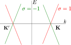
Figure 1: The Dirac spectrum of a metallic nanotube. Each branch is characterized by the isospin value $\sigma$, which is an eigenvalue of the Pauli matrix $\sigma_{2}$. We note that the Kramers partners at $K$ and $K^{\prime}$, respectively, are characterized by the same value of the isospin, and two partner states at the same cone are characterized by opposite isospins.

IV.2 Semiconducting nanotubes

IV.2.1 Zero chemical potential

Now we consider semiconducting CNTs that are characterized by a non-zero circumferential wavevector $k_{G}$ and a corresponding gap in the spectrum. We begin with the case of the Fermi level $\epsilon_{F}$ lying in the middle of the gap, $\epsilon_{F}=0$. As a result, there are no states at the Fermi level. This leads to a strong suppression of the RKKY interaction. For example, the Green function on the same sublattice, found from Eqs. (6) and (9), is given by

$$G^{AA}(\mathbf{R},\tau)\approx-\frac{a}{2\pi} \cos(\mathbf{K}\cdot\mathbf{R})e^{ik_{G}z-\upsilon_{F}|\tau|k_{G}}$$

$$\times\sqrt{\frac{2\pi k_{G}}{\upsilon_{F}|\tau|}}e^{-z^{2}k_{G}/2\upsilon_{F}|\tau|},$$ (20)

where we used the simplified parabolic spectrum, see Eq. (15). The spin susceptibility is then obtained from Eq. (5),

$$\chi^{AA}(\mathbf{R}) =-\frac{2a^{2}k_{G}}{\pi\hbar\upsilon_{F}}\cos^{2}(\mathbf{K}\cdot\mathbf{R})K_{0}(2\sqrt{2}k_{G}|z|),$$ (21)

where $K_{0}(x)$ is the modified Bessel function of second kind, which decays exponentially at large distances, $K_{0}(x)\approx e^{-x}\sqrt{\pi/2x}$ for $x\gg 1$. This exponential decay (on the scale of the CNT diameter $d$) of the spin susceptibility in the case when the Fermi level lies in the gap is not surprising. There are just no delocalized electron states that can assist the effective coupling between two separated localized spins. From now on we neglect any contributions coming from higher or lower bands.

IV.2.2 Non-zero chemical potential

In this subsection we assume that the Fermi level is tuned in such a way that it crosses, for example, the conduction band. Thus, the itinerant states assist the RKKY interaction between localized spins. The spectrum of a semiconducting CNT is parabolic [see Eq. (15)], so it is more convenient to work with the spin susceptibility given by Eq. (4). In momentum space the spin susceptibility on the same sublattice is given by $\chi^{AA}(q)=\sum_{\gamma,\gamma^{\prime}}\chi^{AA}(\gamma,\gamma^{\prime};q)$ with

$$\chi^{AA}(\gamma,\gamma^{\prime};q)=\frac{1}{2}\sum_{k}\frac{\theta[\xi_{\gamma^{\prime}}(k+q)]-\theta[\xi_{\gamma}(k)]}{\xi_{\gamma^{\prime}}(k+q)-\xi_{\gamma}(k)}.$$ (22)

Performing integration over momentum $k$, we arrive at an expression similar to the Lindhard function,

$$\chi^{AA}(\gamma,\gamma^{\prime};q)=-\frac{ak_{G}}{2\pi\hbar\upsilon_{F}q}\ln\left|\frac{q+2k_{F}}{q-2k_{F}}\right|,$$ (23)

where the Fermi momentum $k_{F}$ is defined as $k_{F}=\sqrt{2k_{G}(\epsilon_{F}-\hbar\upsilon_{F}k_{G})/\hbar\upsilon_{F}}$. Next we go to real space by taking the Fourier transform of $\chi^{AA}(\gamma,\gamma^{\prime};q)$. This can be readily done by closing the integration contour in the upper (lower) complex plane for $z>0$ $(z<0)$ and deforming it around the two branch cuts of the logarithm in Eq. (23) that run from $\pm 2k_{F}$ to $\pm\infty$. This yields,

$$\chi^{AA}(\mathbf{R})=\frac{a^{2}k_{G}}{\pi\hbar\upsilon_{F}}{\rm si}(2k_{F}|z|)\left[1+\cos(2\mathbf{K}\cdot\mathbf{R})\right].$$ (24)

Here, the sine integral is defined as

$${\rm si}(x)=\int_{0}^{x}dt\ \frac{\sin t}{t}-\frac{\pi}{2},$$ (25)

and at large distances, $x\gg 1$, its asymptotics is given by ${\rm si}(x)~{}\approx~{}-\cos(x)/x$.

The evaluation of the spin susceptibility for different sublattices is more involved,

$$\chi^{AB}(\gamma,\gamma^{\prime};q)=\frac{\gamma\gamma^{\prime}}{2}\sum_{k}e^{-i\Delta\phi_{k,q}}\frac{\theta[\xi_{\gamma^{\prime}}(k+q)]-\theta[\xi_{\gamma}(k)]}{\xi_{\gamma}(k)-\xi_{\gamma^{\prime}}(k+q)},$$ (26)

where the phase difference given by $\Delta\phi_{k,q}=\phi_{k}-\phi_{k+q}$ depends on the momenta $k$ and $q$, see Eq. (10). Taking into account that $k_{G}$ is the largest momentum characterizing the system, we expand the phase factor as $e^{i(\phi_{k}-\phi_{k+q})}\approx 1-iq/k_{G}$. The main contribution to the spin susceptibility comes from the momentum-independent part and is given by

$$\chi^{AB}(\mathbf{R})=\frac{a^{2}k_{G}}{\pi\hbar\upsilon_{F}}{\rm si}(2k_{F}|z|)\left[1-\cos(2\mathbf{K}\cdot\mathbf{R})\right].$$ (27)

In the next step we evaluate the correction $\Delta\chi^{AB}(\mathbf{R})$ to the spin susceptibility $\chi^{AB}(\mathbf{R})$ arising from the momentum-dependent part in the phase factor $e^{i\Delta\phi_{k,q}}$. In momentum space it is given by

$$\Delta\chi^{AB}(\gamma,\gamma^{\prime};q)=\frac{ia\gamma\gamma^{\prime}}{2\pi\hbar\upsilon_{F}}\ln\left|\frac{q+2k_{F}}{q-2k_{F}}\right|.$$ (28)

By taking the Fourier transform of Eq. (28), we arrive at the following expression,

$$\Delta\chi^{AB}(\mathbf{R})= \sum_{\gamma,\gamma^{\prime}}e^{i(\gamma-\gamma^{\prime})\mathbf{K}\cdot\mathbf{R}}\frac{ia^{2}\gamma\gamma^{\prime}}{2\pi\hbar\upsilon_{F}}$$

$$\times\int^{\infty}_{-\infty}dq\ e^{iqz}\ln\left|\frac{q+2k_{F}}{q-2k_{F}}\right|.$$ (29)

The integral in Eq. (29) can be evaluated easily by recognizing it as the derivative of ${\rm si}(x)$ [see Eq. (23)],

$$I=\int^{\infty}_{-\infty} dx\ e^{i\alpha x}\ln\left|\frac{x+1}{x-1}\right|=-i\frac{\sin\alpha}{|\alpha|},$$ (30)

where $\alpha$ is real. As a result, the correction to the spin susceptibility on different sublattices $\chi^{AB}(\mathbf{R})$ is given by

$$\Delta\chi^{AB}(\mathbf{R})=\frac{a^{2}\sin(2k_{F}z)}{\pi\hbar\upsilon_{F}|z|}\left[1-\cos(2\mathbf{K}\cdot\mathbf{R})\right].$$ (31)

We note that $\Delta\chi^{AB}(\mathbf{R})$ is small in comparison with $\chi^{AB}(\mathbf{R})$ by a factor $k_{F}/k_{G}\ll 1$, and, thus, this correction plays a role only around the points where the oscillating function $\chi^{AB}(\mathbf{R})$ vanishes. We emphasize that the spin susceptibility for semiconducting CNTs does not possess any significant dependence on the sublattices in contrast to metallic CNTs.

V RKKY in the presence of SOI

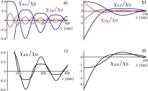
Figure 2: The spin susceptibility $\chi_{\alpha\beta}$, given in Eqs. (44)-(46), plotted as a function of distance between localized spins $z$, for a semiconducting (11,1)-CNT in the presence of spin orbit interaction and at zero B-field. Here, $\chi_{0}=a^{2}k_{G}/2\pi\hbar\upsilon_{F}$. For clarity we suppress the fast oscillating factors and plot only the slowly varying envelopes at small (a,c) and large scales (b,d). The chemical potential $\mu=472\ \rm meV$ ($\delta\mu\equiv\mu-\hbar\upsilon_{F}k_{G}+\beta_{+}=1\ \rm meV$) is tuned inside the gap opened by SOI with corresponding value $2\beta_{+}=1.7\ \rm meV$ for a (11,1)-CNT. cnt_helical_2011 The diagonal components $\chi_{zz}$ [(a,b) blue full curve] and $\chi_{xx}$ (c,d) oscillate with period $2\pi/k_{+,-}\approx 2\pi/k_{F}$. In contrast to that, the off-diagonal component $\chi_{xy}$ [(a,b) red dashed curve], oscillates with period $2\pi/k_{+,+}\approx\pi/k_{F}$. All components decay as $1/z$. Note that the diagonal and off-diagonal components are of comparable size.

In the presence of spin orbit interaction, the spin space is no longer invariant under rotations, and as a consequence the spin susceptibility is described by the tensor $\chi_{\alpha\beta}^{ij}$ [see Eq. (2)] with non-vanishing off-diagonal components. In this case it is more convenient to work in the framework of retarded Green functionsBruno_2004 in which the RKKY Hamiltonian $H_{RKKY}$ is given by Eq. (3). Below we neglect the weak dependence of the susceptibility on the sublattice discussed above and focus on the SOI effects. The Green functions in the energy-momentum space can be expressed as

$$G(k,\epsilon+i0^{+})=\sum_{\gamma}[G_{0}(\gamma,k,\epsilon)+G_{1}(\gamma,k,\epsilon)s_{z}],$$ (32)

where the diagonal and off-diagonal (in spin space) Green functions are given by

$$G_{0}(\gamma,k,\epsilon)=\frac{k_{G}}{\hbar\upsilon_{F}}\sum_{\eta=\pm 1}\frac{1}{k_{\gamma\eta}^{2}-k^{2}+i0^{+}},$$ (33)

$$G_{1}(\gamma,k,\epsilon)=-\frac{k_{G}}{\hbar\upsilon_{F}}\sum_{\eta=\pm 1}\frac{\eta}{k_{\gamma\eta}^{2}-k^{2}+i0^{+}}.$$ (34)

Here, to simplify notations, we introduced the wavevector $k_{\eta^{\prime}}$, defined as (with ${\eta^{\prime}}={\gamma\eta}$)

$$k_{\eta^{\prime}}=\sqrt{2k_{G}(\epsilon-\hbar\upsilon_{F}k_{G}-\eta^{\prime}\beta_{+})/\hbar\upsilon_{F}},$$ (35)

which can take both real and imaginary values. In a next step we transform the Green functions from momentum to real space,

$$G_{0,1}(\mathbf{R},\epsilon+i0^{+})=\frac{a}{2}\sum_{\gamma}\int\frac{dk}{2\pi}G_{0,1}(\gamma,k,\epsilon)e^{i(\gamma\mathbf{K}+\mathbf{k})\cdot\mathbf{R}},$$ (36)

leading to

$$G_{0}(\mathbf{R},\epsilon) =-i\frac{ak_{G}}{2\hbar\upsilon_{F}}\cos(\mathbf{K}\cdot\mathbf{R})\sum_{\eta=\pm 1}\frac{e^{ik_{\eta}|z|}}{k_{\eta}+i0^{+}},$$ (37)

$$G_{1}(\mathbf{R},\epsilon) =\frac{ak_{G}}{2\hbar\upsilon_{F}}\sin(\mathbf{K}\cdot\mathbf{R})\sum_{\eta=\pm 1}\frac{\eta e^{ik_{\eta}|z|}}{k_{\eta}+i0^{+}}.$$ (38)

Substituting $G(\mathbf{R},\epsilon)=G_{0}(\mathbf{R},\epsilon)+G_{1}(\mathbf{R},\epsilon)s_{z}$ into Eq. (3), we find for the RKKY Hamiltonian,

$$H {}_{RKKY}=-\frac{J^{2}}{\pi}{\rm Im}\left[-4I_{i}^{z}I_{j}^{z}\int_{-\infty}^{\epsilon_{F}}d\epsilon\ G^{2}_{1}(\mathbf{R},\epsilon)\right.$$

$$\left.-4i(\mathbf{I}_{i}\times\mathbf{I}_{j})_{z}\int_{-\infty}^{\epsilon_{F}}d\epsilon\ G_{1}(\mathbf{R},\epsilon)G_{0}(\mathbf{R},\epsilon)\right.$$

$$\left.+2\mathbf{I}_{i}\cdot\mathbf{I}_{j}\int_{-\infty}^{\epsilon_{F}}d\epsilon\ \left[G^{2}_{0}(\mathbf{R},\epsilon)+G^{2}_{1}(\mathbf{R},\epsilon)\right]\right].$$ (39)

Here, the trace over spin degrees of freedom were calculated by using the following identities

$${\rm Tr}\{(\mathbf{I}_{i}\cdot\boldsymbol{s})(\mathbf{I}_{j}\cdot\boldsymbol{s})\}=2\mathbf{I}_{i}\cdot\mathbf{I}_{j},$$ (40)

$${\rm Tr}\{(\mathbf{I}_{i}\cdot\boldsymbol{s})s_{z}(\mathbf{I}_{j}\cdot\boldsymbol{s})\}=-2i(\mathbf{I}_{i}\times\mathbf{I}_{j})_{z},$$ (41)

$${\rm Tr}\{(\mathbf{I}_{i}\cdot\boldsymbol{s})s_{z}(\mathbf{I}_{j}\cdot\boldsymbol{s})s_{z}\}=2(2I_{i}^{z}I_{j}^{z}-\mathbf{I}_{i}\cdot\mathbf{I}_{j}).$$ (42)

All integrals in Eq. (39) are of the same type,

$${\rm Im}\int_{-\infty}^{\epsilon_{F}}d\epsilon\ \frac{e^{ik_{\eta}|z|}}{k_{\eta}+i0^{+}}\frac{e^{ik_{\eta^{\prime}}|z|}}{k_{\eta^{\prime}}+i0^{+}}=\frac{\hbar\upsilon_{F}}{k_{G}}{\rm si}(k_{\eta\eta^{\prime}}|z|),$$ (43)

and can be easily evaluated by changing variables from the original $\epsilon$ to $k_{\eta}+k_{\eta^{\prime}}$ . We denote the real part of the sum of two Fermi wavevectors as $k_{\eta,\eta^{\prime}}={\rm Re}[k_{\eta}(\epsilon_{F})+k_{\eta^{\prime}}(\epsilon_{F})]$ with the indices $\eta,\eta^{\prime}=\pm 1$. As a result, we arrive at the RKKY Hamiltonian in the form of Eq. (2), where the components of the spin susceptibility tensor $\chi^{ij}_{\alpha\beta}\equiv\chi_{\alpha\beta}(\mathbf{R})$ are explicitly given by

$$\chi_{zz}=\frac{a^{2}k_{G}}{2\pi\hbar\upsilon_{F}}\Big{[}{\rm si}(k_{+,+}|z|)+{\rm si}(k_{-,-}|z|)$$

$$\ \ \ \ \ \ \ \ \ \ \ \ \ \ \ \ \ \ +2\cos(2\mathbf{K}\cdot\mathbf{R}){\rm si}(k_{-,+}|z|)\Big{]},$$ (44)

$$\chi_{xx}=\frac{a^{2}k_{G}}{2\pi\hbar\upsilon_{F}}\Big{(}2{\rm si}(k_{-,+}|z|)+\cos(2\mathbf{K}\cdot\mathbf{R})$$

$$\ \ \ \ \ \ \ \ \ \ \ \ \ \ \ \ \ \ \ \ \times[{\rm si}(k_{+,+}|z|)+{\rm si}(k_{-,-}|z|)]\Big{)},$$ (45)

$$\chi_{xy}=\frac{a^{2}k_{G}}{2\pi\hbar\upsilon_{F}}\sin(2\mathbf{K}\cdot\mathbf{R})$$

$$\ \ \ \ \ \ \ \ \ \ \ \ \ \ \ \ \ \ \ \ \times\Big{[}{\rm si}(k_{+,+}|z|)-{\rm si}(k_{-,-}|z|)\Big{]},$$ (46)

with $\chi_{xx}=\chi_{yy}$, $\chi_{xy}=-\chi_{yx}$, and all other components being zero. First, we note that the off-diagonal components $\chi_{xy},\chi_{yx}$ are non-zero. They describe the response to a perturbation applied perpendicular to the nanotube axis. This opens up the possibility to test the presence of SOI in the system by measuring off-diagonal components of the spin susceptibility tensor $\chi_{\alpha\beta}$. Second, the spin response in a direction perpendicular to the $z$-axis cannot be caused by a perturbation along the $z$-axis, thus $\chi_{yz}=\chi_{xz}=0$. This simply reflects the rotation-invariance of CNTs around their axes. The difference between the diagonal elements of the spin susceptibility tensor, $\chi_{xx}=\chi_{yy}$ and $\chi_{zz}$, again arises from the SOI and is another manifestation of the broken rotation invariance of spin space. In total this means that the RKKY interaction given in Eq. (39) is anisotropic in the presence of SOI, giving rise to an Ising term $\propto I_{i}^{z}I_{j}^{z}$ and a Moryia-Dzyaloshinsky term $\propto(\mathbf{I}_{i}\times\mathbf{I}_{j})_{z}$, in addition to the isotropic Heisenberg term $\propto\mathbf{I}_{i}\cdot\mathbf{I}_{j}$.

Quite remarkably, when the Fermi level is tuned close to the gap opened by the SOI, then the off-diagonal and diagonal components of the susceptibility tensor become of comparable magnitude, see Figs. 2 and 3. This has important consequences for a Kondo lattice system, where a highly anisotropic RKKY interaction will give rise to an ordered magnetic phase even at finite temperatures.order_2_2011 As a potential candidate for such a Kondo lattice Braunecker_2009_PRB we might mention a CNT made out of the ${}^{13}C$-isotope, Churchill_2009 where each site of the graphene lattice contains a nuclear spin-1/2 to which the itinerant electrons couple via hyperfine interaction. Fischer_2009

We note that the susceptibility depends on two Fermi wavevectors via $k_{\eta\eta^{\prime}}$ in a rather complicated way (see Figs. 2 and 3). In the absence of SOI, we recover the result for the spin susceptibility on the same sublattice, $\chi^{AA}(\mathbf{R})$ [see Eq. (24)]. The leading term in the spin susceptibility for different sublattices, $\chi^{AB}(\mathbf{R})$, can be obtained from Eqs. (44) - (46) by putting a minus sign in front of $\cos(2\mathbf{K}\cdot\mathbf{R})$. In addition, as shown in Sec. IV.2, the spin susceptibility vanishes if the Fermi level is tuned inside the gap in semiconducting CNTs, so that both $k_{\pm}(\epsilon_{F})$ are purely imaginary. If the chemical potential is inside the gap opened by the SOI, the Fermi wavevector $k_{-}(\epsilon_{F})$ is still imaginary, at the same time $k_{+}(\epsilon_{F})$ is real, giving $k_{+,+}=2k_{+}(\epsilon_{F})$, $k_{-,-}=0$, and $k_{+,-}=k_{+}(\epsilon_{F})$. This results in the behavior of the spin susceptibility shown in Fig. 2. The strength of the RKKY interaction decays oscillating as $1/R$. The oscillation period is determined by $k_{+,+}$ for $\chi_{xy}$ and by $k_{+,-}$ for $\chi_{xx}$ and $\chi_{zz}$, see Fig. 2. If the chemical potential is above the SOI gap, then both wavevectors $k_{\pm}(\epsilon_{F})$ are real, giving rise to oscillations with two different frequencies that result in beating patterns for the spin susceptibility, see Fig. 3.

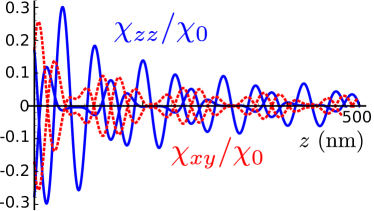
Figure 3: The same as Fig. 2 (a,b) but with the chemical potential $\mu=474\ \rm meV$ being tuned above the gap opened by SOI. The spin susceptibility decays as $1/z$ and exhibits beatings, with period determined by the SOI parameters.

VI RKKY with magnetic field

In Sec. V we demonstrated that the presence of SOI, which breaks rotation invariance in spin space, leads to an anisotropic spin susceptibility. Another way to break this rotation invariance is to apply a magnetic field, which also breaks time-reversal invariance. In this section we again neglect sublattice asymmetries discussed above and focus on the effects of a magnetic field $\bf B$ applied along the nanotube axis $z$ for a semiconducting nanotube. The Zeeman term $H_{Z}=\Delta_{Z}s_{z}=\mu_{B}Bs_{z}$ lifts the spin degeneracy. Here, $\mu_{B}$ is the Bohr magneton. The orbital term $H_{orb}=\gamma\hbar\upsilon_{F}k_{mag}$ leads to a shift of the transverse wavevector $k_{G}$ by $k_{mag}$, which finds its origin in the Aharonov-Bohm effect and is given by $k_{mag}=\pi Bd|e|/2h$ for a nanotube of diameter $d$. Thus, the valley degeneracy of the levels is also lifted. The spectrum of the effective Hamiltonian $H_{0}+H_{Z}+H_{orb}$ in the case of a semiconducting nanotube is given by

$$\epsilon_{\gamma,s}=\hbar\upsilon_{F}k_{G,\gamma}+s(\gamma\beta_{+}+\Delta_{z})+\hbar\upsilon_{F}k^{2}/2k_{G,\gamma},$$ (47)

where $k_{G,\gamma}=k_{G}+\gamma k_{mag}$. The Green functions in momentum space can be found similar to Eq. (32). As a result, we arrive at the following expression for the Green functions,

$$G(k,\epsilon+i0^{+})=\sum_{\gamma}[G_{0}(\gamma,k,\epsilon)+G_{1}(\gamma,k,\epsilon)s_{z}],$$ (48)

where

$$G_{0}(\gamma,k,\epsilon)=\frac{k_{G,\gamma}}{\hbar\upsilon_{F}}\sum_{s}\frac{1}{\kappa_{\gamma,s}^{2}-k^{2}+i0^{+}},$$ (49)

$$G_{1}(\gamma,k,\epsilon)=-\frac{k_{G,\gamma}}{\hbar\upsilon_{F}}\sum_{s}\frac{s}{\kappa_{\gamma,s}^{2}-k^{2}+i0^{+}}.$$ (50)

Here, we define wavevectors $\kappa_{\gamma,s}$ as a function of the energy $\epsilon$ from Eq. (47) as

$$\kappa_{\gamma,s}=\sqrt{\frac{2k_{G,\gamma}[\epsilon-\hbar\upsilon_{F}k_{G,\gamma}-s(\gamma\beta_{+}+\Delta_{z})]}{\hbar\upsilon_{F}}},$$ (51)

which can take both non-negative real and imaginary values. The Green functions in real space are found by Fourier transformation,

$$G_{0}(\mathbf{R},\epsilon) =-i\sum_{\gamma,s}\frac{ak_{G,\gamma}}{2\hbar\upsilon_{F}}e^{i\gamma\mathbf{K}\cdot\mathbf{R}}\frac{e^{i\kappa_{\gamma,s}|z|}}{\kappa_{\gamma,s}+i0^{+}},$$ (52)

$$G_{1}(\mathbf{R},\epsilon) =-i\sum_{\gamma,s}\frac{ak_{G,\gamma}}{2\hbar\upsilon_{F}}e^{i\gamma\mathbf{K}\cdot\mathbf{R}}\frac{se^{i\kappa_{\gamma,s}|z|}}{\kappa_{\gamma,s}+i0^{+}}.$$ (53)

By substituting Eqs. (52) and (53) into Eq. (39), we arrive at the effective RKKY Hamiltonian. Since $k_{mag}/k_{G}\ll 1$, we can neglect the dependence of the spectrum slope on the magnetic field, which simplifies the calculations considerably.

At the end we arrive at the following expressions for the spin susceptibility tensor components

$$\chi_{xx}=\frac{a^{2}k_{G}}{4\pi\hbar\upsilon_{F}}$$

$$\times\sum_{\gamma,s}\Big{[}{\rm si}(k_{\gamma,s;\gamma,\bar{s}}|z|)+\cos(2\mathbf{K}\cdot\mathbf{R}){\rm si}(k_{\gamma,s;\bar{\gamma},\bar{s}}|z|)\Big{]},$$ (54)

$$\chi_{zz}=\frac{a^{2}k_{G}}{4\pi\hbar\upsilon_{F}}$$

$$\times\sum_{\gamma,s}\Big{[}{\rm si}(k_{\gamma,s;\gamma,s}|z|)+\cos[2\mathbf{K}\cdot\mathbf{R}]{\rm si}(k_{\gamma,s;\bar{\gamma},s}|z|)\Big{]},$$ (55)

$$\chi_{xy}=\frac{a^{2}k_{G}}{4\pi\hbar\upsilon_{F}}\sum_{\gamma,s}\gamma s\sin[2\mathbf{K}\cdot\mathbf{R}]{\rm si}(k_{\gamma,s;\bar{\gamma},\bar{s}}|z|),$$ (56)

with $\chi_{xx}=\chi_{yy}$, $\chi_{xy}=-\chi_{yx}$, and the rest being zero. Here, we use the notation $k_{\gamma,s;\gamma^{\prime},s^{\prime}}={\rm Re}[\kappa_{\gamma,s}(\epsilon_{F})+\kappa_{\gamma^{\prime},s^{\prime}}(\epsilon_{F})]$. Again, the RKKY interaction decays at large distances as $1/R$. The spin susceptibility also exhibits oscillations and beating patterns (similar to ones shown in Fig. 3) determined by four different Fermi wavevectors $k_{\gamma s}(\epsilon_{F})$, see Fig. 4. Finally, we note that the same beating patterns arises also for nanowires with parabolic spectrum in the presence of a magnetic field giving rise to a Zeeman splitting.

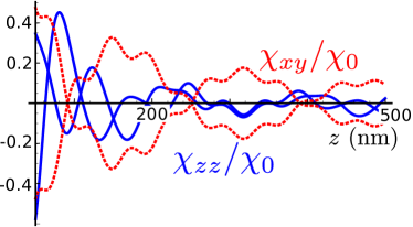
Figure 4: The same as Fig. 2 (a,b) but with the chemical potential $\mu=472.7\ \rm meV$ being tuned in such a way that there are three pairs of states at the Fermi level and with a magnetic field $B=1\ {\rm T}$. The spin susceptibility decays as $1/z$ and exhibits beatings, with period determined by the SOI parameters and the magnetic field.

VII Spin Fluctuations

The spin susceptibility is a fundamental characteristics of the system. At zero frequency it describes the RKKY interaction between localized spins. At finite frequencies $\omega$ the spin susceptibility gives access to the equilibrium spin noise in the system. For a general observable, $s_{\alpha}$, the fluctuation-dissipation theoremgiuliani_book connects the dynamical structure factor $S_{\alpha\alpha}({\bf q},\omega)=(1/2\pi)\int dt\ \langle s_{\alpha}({\bf q},t)s_{\alpha}({\bf-q},0)\rangle e^{i\omega t}$, describing equilibrium fluctuations, with the linear response susceptibility, $\chi_{\alpha\alpha}({\bf q},\omega)=(-i/\hbar)\int dt\ \Theta(t)\langle[s_{\alpha}({\bf q},t),s_{\alpha}({\bf-q},0)]\rangle e^{i\omega t}$,

$${\rm Im}\chi_{\alpha\alpha}({\bf q},\omega)=\frac{\pi}{\hbar}(e^{-\frac{\hbar\omega}{k_{B}T}}-1)S_{\alpha\alpha}({\bf q},\omega)\,,$$ (57)

for $\omega>0$. Below we calculate the spin susceptibility for both metallic and semiconducting nanotubes at finite frequencies, and obtain via Eq. (57) the spin correlation function (spin noise) $S_{\alpha\alpha}(\mathbf{R},\omega)$ in real space at zero temperature,

$$S_{\alpha\alpha}(\mathbf{R},\omega)=-\frac{\hbar}{\pi}\ {\rm Im}\chi_{\alpha\alpha}({\bf R},\omega),$$ (58)

Here, we assumed that the system is invariant under parity transformation so that $\chi({\bf q},\omega)$ becomes an even function of ${\bf q}$. For simplicity, we consider only the case without SOI.

VII.1 Metallic nanotubes

The spin susceptibility at finite Matsubara frequencies $\omega_{n}$ is given by

$$\chi_{0}(\mathbf{R},i\omega_{n})=\frac{2}{{\hbar}}\int_{0}^{\infty}d\tau\ G_{0}(\mathbf{R},\tau)G_{0}(-\mathbf{R},-\tau)e^{i\omega_{n}\tau},$$ (59)

where we modified Eq. (5) accordingly, and the Green function $G_{0}(\mathbf{R},\tau)$ was found before [see Eqs. (16) and (17)]. For the spin susceptibility on the same sublattice we get

$$\chi^{AA}_{0}(\mathbf{R},i\omega_{n})=\frac{2a^{2}}{\pi^{2}\hbar}\cos^{2}(\mathbf{K}\cdot\mathbf{R})$$

$$\times\int_{0}^{\infty}d\tau\ e^{i\omega_{n}\tau}\frac{[z\sin(k_{F}z)]^{2}-[v_{F}\tau\cos(k_{F}z)]^{2}}{[(v_{F}\tau)^{2}+z^{2}]^{2}}.$$ (60)

Introducing the notation

$$I_{n}(x)=\int_{0}^{\infty}d\tau\ \frac{\tau^{n}e^{i\tau x}}{(1+\tau^{2})^{2}}\,,$$ (61)

where $n=0,2$, the susceptibility can be rewritten as

$$\chi_{0}^{AA}(\mathbf{R},i\omega_{n})=\frac{2a^{2}}{\pi^{2}\hbar v_{F}|z|}\cos^{2}(\mathbf{K}\cdot\mathbf{R})$$

$$\times\left[\sin^{2}(k_{F}z)I_{0}\left(\frac{\omega_{n}|z|}{v_{F}}\right)-\cos^{2}(k_{F}z)I_{2}\left(\frac{\omega_{n}|z|}{v_{F}}\right)\right].$$ (62)

The asymptotics of $I_{n}(x)$ for small $x$ is given by $I_{0}(x)\approx\pi/4+ix/2$ and $I_{2}(x)\approx\pi(1-2x)/4-ix(\ln x+\gamma_{e}-1/2)$, where $\gamma_{e}$ is the Euler constant. Performing the standard analytic continuation from Matsubara to real frequencies, giuliani_book we obtain the spin susceptibility $\chi^{AA}_{0}(\omega)$, and from its imaginary part the spin noise, see Eq. (58). Explicitly, the dynamical structure factor at zero temperature and for ${v_{F}}\gg{\omega|z|}\geq 0$ is given by

$$S^{AA}(\mathbf{R},\omega)=-\frac{2a^{2}\omega}{\pi^{2}v_{F}^{2}}\cos^{2}(\mathbf{K}\cdot\mathbf{R})\cos^{2}(k_{F}z).$$ (63)

For the susceptibility on different sublattices we find

$$\chi^{AB}_{0}(\mathbf{R},i\omega_{n})=-\frac{2a^{2}}{\pi^{2}\hbar v_{F}|z|}\sin^{2}(\mathbf{K}\cdot\mathbf{R})$$

$$\times\left[\sin^{2}(k_{F}z)I_{2}\left(\frac{\omega_{n}|z|}{v_{F}}\right)-\cos^{2}(k_{F}z)I_{0}\left(\frac{\omega_{n}|z|}{v_{F}}\right)\right],$$ (64)

with the corresponding dynamical structure factor being given by

$$S^{AB}(\mathbf{R},\omega)=-\frac{2a^{2}\omega}{\pi^{2}v_{F}^{2}}\sin^{2}(\mathbf{K}\cdot\mathbf{R})\sin^{2}(k_{F}z).$$ (65)

The dynamical structure factors $S^{AA}(\mathbf{R},\omega)$ and $S^{AB}(\mathbf{R},\omega)$ are linear in $\omega$, and, as expected, vanish at zero frequency (we recall that we work at zero temperature). Moreover, the noise is strongly suppressed at some special points $R_{z}$ in space that satisfy the condition $k_{F}z=n\pi/2$, where $n$ is an integer.

In the opposite limit ${\omega|z|}\gg{v_{F}}$ we use the following asymptotics, $I_{0}(x)\approx i/x+\pi xe^{-x}/2$ and $I_{2}(x)\approx-2i/x^{3}-\pi xe^{-x}/2$ for $x\gg 1$. After analytic continuation, the dynamical structure factor is then given by

$$S^{AA}(\mathbf{R},\omega)= \frac{a^{2}\omega}{\pi^{2}v_{F}^{2}}\cos^{2}(\mathbf{K}\cdot\mathbf{R})\cos\left(\frac{\omega|z|}{v_{F}}\right),$$ (66)

$$S^{AB}(\mathbf{R},\omega)= \frac{a^{2}\omega}{\pi^{2}v_{F}^{2}}\sin^{2}(\mathbf{K}\cdot\mathbf{R})\cos\left(\frac{\omega|z|}{v_{F}}\right).$$ (67)

In this regime, $S^{AA}(\mathbf{R},\omega)$ and $S^{AB}(\mathbf{R},\omega)$ are not only linearly proportional to the frequency but also oscillate rapidly as a function of frequency. This implies that in real time the spin noise is only non-zero for times $t$ and distances $z$ satisfying $|z|=v_{F}t$.

VII.2 Semiconducting nanotubes

For semiconducting CNTs all calculations for the frequency dependent susceptibility are similar to the ones for one-dimensional systems with parabolic spectrum, being available in the literature. giuliani_book At zero temperature ${\rm Im}\chi_{\alpha\alpha}({q},\omega)$ is given by

$${\rm Im}\chi_{\alpha\alpha}({q},\gamma,\gamma^{\prime},\omega)=-\frac{\pi}{2}\sum_{k}\left[\theta(\xi_{k,\gamma})-\theta(\xi_{k+q,s,\gamma^{\prime}})\right]$$

$$\hskip 80.0pt\times\delta(\hbar\omega+\xi_{k,s,\gamma}-\xi_{k+q,s,\gamma^{\prime}}).$$ (68)

The upper and lower frequencies $\omega_{\pm}$ are defined as

$$\omega_{\pm}(q)=\left|\frac{\upsilon_{F}q^{2}}{2k_{G}}\pm\frac{\upsilon_{F}k_{F}}{k_{G}}|q|\right|.$$ (69)

The imaginary part of the spin susceptibility is non-zero only for frequencies

$$\omega_{-}(q)\leq|\omega|\leq\omega_{+}(q)$$ (70)

and is given by

$${\rm Im}\chi_{\alpha\alpha}({q},\gamma,\gamma^{\prime},\omega)=-\frac{ak_{G}}{4\hbar\upsilon_{F}|q|}{\rm sgn}(\omega).$$ (71)

To arrive at the expression in real space we perform the Fourier transformation,

$${\rm Im}\chi_{\alpha\alpha}(\mathbf{R},\omega)=(1\pm\cos(2\mathbf{K}\cdot\mathbf{R}))$$

$$\hskip 50.0pt\times\frac{a^{2}k_{G}}{4\pi\hbar\upsilon_{F}}{\rm Im}\int dq\ \frac{e^{iqz}}{|q|}{\rm sgn}(\omega),$$ (72)

where the range of the $q$-integration is determined from Eq. (70), and the positive (negative) sign corresponds to $\chi^{AA}_{\alpha\alpha}$ ($\chi^{AB}_{\alpha\alpha}$). For high frequencies, $\omega>\upsilon_{F}k_{F}^{2}/2k_{G}$, the dynamical structure factor is given by

$$S(\mathbf{R},\omega)=(1\pm\cos(2\mathbf{K}\cdot\mathbf{R}))\frac{a^{2}k_{G}}{2\pi^{2}\upsilon_{F}}$$

$$\hskip 40.0pt\times\left[{\rm si}(q_{+}(\omega)|z|)-{\rm si}(q_{-}(\omega)|z|)\right]{\rm sgn}(\omega),$$ (73)

where wavevectors $q_{\pm}(\omega)$ are positive solutions of the equations $|\omega|=|\omega_{\pm}(q_{\pm})|$. For low frequencies, $0<\omega\leq\upsilon_{F}k_{F}^{2}/2k_{G}$, the same equation $|\omega|=|\omega_{-}(q_{-,i})|$ has three non-negative solutions, giuliani_book $q_{-,1}\leq q_{-,2}\leq q_{-,3}$. In this case $S(\mathbf{R},\omega)$ is given by

$$S(\mathbf{R},\omega)=(1\pm\cos(2\mathbf{K}\cdot\mathbf{R}))\frac{a^{2}k_{G}}{2\pi^{2}\upsilon_{F}}{\rm sgn}(\omega)$$

$$\hskip 40.0pt\times[{\rm si}(q_{+}(\omega)|z|)-{\rm si}(q_{-,1}(\omega)|z|)$$

$$\hskip 60.0pt+{\rm si}(q_{-,2}(\omega)|z|)-{\rm si}(q_{-,3}(\omega)|z|)].$$ (74)

We note that the expression is composed of several contributions and thus leads to beating patterns of the spin noise, similar to the one before for the spin susceptibility.

VIII Graphene nanoribbons

VIII.1 The effective Hamiltonian

In the last part of this work, we turn to graphene nanoribbons, which are finite-size sheets of graphene.brey_2006 The nanoribbon is assumed to be aligned along the $z$-direction and to have a finite width $W=Na$ in $x$-direction, with $N$ being the number of unit cells in this transverse direction. Here, we focus on armchair nanoribbons, characterized by the fact that the $x$-axis points along one of the translation vectors of the graphene lattice. The effective Hamiltonian is given by

$$H_{0}=\hbar\upsilon_{F}(\gamma k_{x}\sigma_{1}+k_{z}\sigma_{2})\,,$$ (75)

which determines the low-energy spectrum around the two Dirac points ${\bf K}=-{\bf K}^{\prime}=(4\pi/3a,0)$. Here, $k_{z}$ is the momentum in $z$-direction. The momentum $k_{x}$ in $x$-direction is quantized due to the vanishing boundary conditions imposed on the extended nanoribbon.brey_2006 If the width of the GNR is such that $N=3M+~{}1$, where $M$ is a positive integer, the GNR is metallic with $k_{x}=0$. Otherwise, the nanoribbon is semiconducting.

The eigenstates are written as $\psi=\sum_{\sigma\gamma}\phi_{\sigma\gamma}e^{i\gamma K_{x}x}$, $\Phi=(\phi_{AK},\phi_{BK},\phi_{AK^{\prime}},\phi_{BK^{\prime}})$, where $\sigma=A,B$. The corresponding spectrum and wavefunctions that satisfy the vanishing boundary conditions (for $\psi$) are given by

$$\Phi^{\epsilon,k_{z}}_{\zeta}=e^{ik_{z}z}(-i\zeta,1,i\zeta,-1),$$ (76)

$$\epsilon_{\zeta}=\zeta\hbar\upsilon_{F}k_{z}$$ (77)

for a metallic GNR, and

$$\Phi^{\epsilon,k_{z}}_{\pm}=e^{ik_{z}z}(\pm e^{i\varphi_{s}+ixk_{x}^{min}},e^{ixk_{x}^{min}},$$

$$\ \ \ \ \ \ \ \ \ \ \ \ \ \ \ \ \ \ \ \ \ \ \ \ \ \mp e^{i\varphi_{s}-ixk_{x}^{min}},-e^{-ixk_{x}^{min}}),$$ (78)

$$\epsilon_{\pm}=\pm\hbar\upsilon_{F}\sqrt{(k_{x}^{min})^{2}+k_{z}^{2}}$$ (79)

for a semiconducting GNR. Here, $\zeta=\pm 1$ is the eigenvalue of the Pauli matrix $\sigma_{2}$, and we use the notation $e^{i\varphi_{s}}=[k_{x}^{min}-ik_{z}]/\sqrt{(k_{x}^{min})^{2}+k_{z}^{2}}$, with $|k_{x}^{min}|=\pi/3(N+2)a$.

VIII.2 Spin susceptibility

VIII.2.1 Without SOI

To calculate the spin susceptibility for a metallic nanoribbon that has a linear spectrum given by Eq. (77), we again work in the imaginary time formalism, see Eq. (5). The calculations are quite similar to the ones presented before in Sec. IV.1. The only change in the expressions for the spin susceptibility in comparison with a metallic nanotube [see Eqs. (18) and (19)] is in the fast oscillating prefactor,

$$\chi_{0}^{AA}(\mathbf{R}_{i}, \mathbf{R}_{j})=-\chi_{0}^{AB}(\mathbf{R}_{i},\mathbf{R}_{j})=-\frac{a^{2}}{2\pi\hbar v_{F}|z|}$$

$$\times\sin^{2}(\mathbf{K}\cdot\mathbf{R}_{i})\sin^{2}(\mathbf{K}\cdot\mathbf{R}_{j})\cos(2k_{F}z).$$ (80)

Similarly, for semiconducting nanoribbons the spin susceptibility is given by Eqs. (24) and (27), where the fast oscillating prefactors $1\pm\cos(2\mathbf{K}\cdot\mathbf{R})$ are replaced by $\sin^{2}(\mathbf{K}\cdot\mathbf{R}_{i})\sin^{2}(\mathbf{K}\cdot\mathbf{R}_{j})$.

VIII.2.2 With SOI

The intrinsic SOI in graphene is only several $\mu eV$, so it is rather weak. Moreover, the Rashba SOI generated by an externally applied electric field $E$ is in the range of tenths of $\mu eV$ for $E=1\ \rm{V/nm}$. cnt_helical_2011 ; klinovaja_MF_CNT Such small SOI values might be hard to observe. However, the Rashba SOI generated by a spatially varying magnetic field opens new perspectives for spintronics in graphene. klinovaja_Nanoribbon In this case, the SOI strength can be exceptionally large, reaching hundreds of $\rm{meV}$. A nanoribbon in the presence of a rotating magnetic field with period $2\pi/k_{n}$, described by the Zeeman Hamiltonian

$$H_{n}^{\perp}=\Delta_{Z}\left[s_{y}\cos(k_{n}z)+s_{z}\sin(k_{n}z)\right],$$ (81)

is equivalent to a nanoribbon with Rashba SOI in the presence of a uniform magnetic field,

$$H^{\perp} =U_{n}^{\dagger}(H_{0}+H_{n}^{\perp})U_{n}=H_{0}+\Delta_{Z}s_{y}+\Delta_{so}^{n}s_{x}\sigma_{2},$$ (82)

where the unitary gauge transformation is given by $U_{n}=\exp(ik_{n}zs_{x}/2)$. The period of the magnetic field determines the strength of the Rashba SOI $\Delta_{so}^{n}=\hbar\upsilon_{F}k_{n}/2$, while the amplitudes of the uniform and the rotating fields are the same and given by $\Delta_{Z}$.Braunecker_Jap_Klin_2009 ; klinovaja_Nanoribbon The spectrum of a metallic (semiconducting) GNR in the presence of such SOI consists of two cones (parabolas) shifted along the momentum axis against each other by $k_{n}/2$. Every branch of the spectrum possesses a well-defined spin polarization perpendicular to the $z$-axis that is along the nanoribbon. A uniform magnetic field only slightly modifies the spectrum by opening a gap at zero momentum. In the following discussion we neglect the uniform magnetic field working in the regime where the induced Rashba SOI is stronger than the Zeeman energy $2\Delta_{Z}$.

As a result, similar to the semiconducting nanowire, one can gauge away the momentum shifts by rotating the spin coordinate system as follows,

$$I_{x}(\mathbf{R})=I_{x}\cos(k_{n}z)+I_{y}\sin(k_{n}z),$$ (83)

$$I_{y}(\mathbf{R})=I_{y}\cos(k_{n}z)-I_{x}\sin(k_{n}z),$$ (84)

$$I_{z}(\mathbf{R})=I_{z}.$$ (85)

The same transformation should be applied to the electron spin operators $\hbar{\bf s}/2$. The effective RKKY Hamiltonian in this rotated coordinate system is the same as in the system without SOI and is given by Eq. (80). To return to the laboratory frame, we perform the following change

$$\mathbf{I}_{i}\cdot\mathbf{I}_{j} \rightarrow\mathbf{I}_{i}(\mathbf{R}_{i})\cdot\mathbf{I}_{j}(\mathbf{R}_{j})=\cos(k_{n}z)\mathbf{I}_{i}\cdot\mathbf{I}_{j}$$

$$+[1-\cos(k_{n}z)]I^{z}_{i}I^{z}_{j}-\sin(k_{n}z)(\mathbf{I}_{i}\times\mathbf{I}_{j})_{z}.$$ (86)

The spin susceptibility tensor has non-vanishing off-diagonal components, which, again, indicate a broken invariance of spin space induced by the magnetic field or the Rashba SOI. As before, this gives rise to anisotropic RKKY interactions of Ising and Moryia-Dzyaloshinski form.

IX Conclusions

In the present work we studied the Rudermann-Kittel-Kasuya-Yosida (RKKY) interaction in carbon nanotubes and graphene nanoribbons at zero temperature in the presence of spin orbit interaction. Our main results are summarized in the following.

The spin susceptibility in metallic CNTs, characterized by a Dirac spectrum (gapless and linear), crucially depends on whether the localized spins that interact with each other are from the same or from different sublattices. In particular, if the Fermi level is tuned exactly to the Dirac point where the chemical potential is zero the interaction is of ferromagnetic type for spins on $A$-$A$ or $B$-$B$ lattice sites, whereas it is of antiferromagnetic type for spins on $A$-$B$ lattice sites. In semiconducting CNTs, with a sizable bandgap, the spin susceptibility depends only slightly on the sublattices. In all cases, the spin susceptibility is an oscillating function that decays as $1/R$, where $R$ is the distance between the localized spins.

The spin orbit interaction breaks the spin degeneracy of the spectrum and the direction invariance of the spin space. As a result, the spin susceptibility is described by the tensor $\chi_{\alpha\beta}$ that has two non-zero off-diagonal components $\chi_{xy}=-\chi_{yx}$, the finite values of which signal the presence of SOI in the system. Moreover, the RKKY interaction is also anisotropic in the diagonal terms, $\chi_{zz}\neq\chi_{xx}=\chi_{yy}$. Quite surprisingly, we find that all non-zero components, diagonal and off-diagonal, can be tuned to be of equal strength by adjusting the Fermi level. These anisotropies, giving rise to Ising and Moriya-Dzyaloshinski RKKY interactions, thus open the possibility to have magnetic order in low-dimensional systems at finite temperature. order_2_2011

We note that, in contrast to semiconducting nanowires, the SOI cannot be gauged away by a unitary transformation in CNTs, giving rise to a more complicated dependence of $\chi_{\alpha\beta}$ on the SOI parameters. In the same way, a magnetic field along the CNT axis breaks both the spin and the valley degeneracy, leading to a dependence of the spin susceptibility on four different Fermi wavevectors.

The spin susceptibility at finite frequencies also allows us to analyze the spin noise in the system via the fluctuation-dissipation theorem. We find that the dynamical structure factor $S_{\alpha\alpha}(\mathbf{R},\omega)$ is linear in frequency and oscillates in real space.

Metallic armchair GNRs behave similarly to metallic CNTs. Indeed, in both cases the spin susceptibility shows a strong dependence on the sublattices, with, however, different fast oscillating prefactors. A Rashba-like SOI interaction can be generated in armchair GNR by periodic magnetic fields. In contrast to CNTs with intrinsic SOI, this field-generated SOI can be gauged away giving rise to a simple structure of the spin susceptibility tensor.note_bilayer

In this work we have ignored interaction effects. However, it is well-known that in one- and two-dimensional systems electron-electron interactions can lead to interesting modifications of the spin susceptibility, for instance with a slower power law decay such as $1/R^{g}$, with $0<g\leq 1$ in a Luttinger liquid approach to interacting one-dimensional wires. Egger_1996 ; Braunecker_2009_PRL It would be interesting to extend the present analysis and to allow for interaction effectsImambekov_RMF in the spin susceptibility for carbon based materials in the presence of spin orbit interaction, in particular for metallic CNTs and GNRs at the Dirac point.

- (1) M. A. Ruderman and C. Kittel, Phys. Rev. B 96, 99 (1954).
- (2) T. Kasuya, Prog. Theor. Phys. 16, 45 (1956).
- (3) K. Yosida, Phys. Rev. 106, 893 (1957).
- (4) N. J. Craig, J. M. Taylor, E. A. Lester, C. M. Marcus, M. P. Hanson, and A. C. Gossard, Science 304, 565 (2004).
- (5) Y. Rikitake and H. Imamura, Phys. Rev. B 72, 033308 (2005).
- (6) D. S. Wang, A. G. Fowler, and L. C. L. Hollenberg, Phys. Rev. A 83, 020302 (2011).
- (7) L. Trifunovic, O. Dial, M. Trif, J. R. Wootton, R. Abebe, A. Yacoby, and D. Loss, Phys. Rev. X 2, 011006 (2012).
- (8) B. Braunecker, P. Simon, and D. Loss, Phys. Rev. Lett. 102, 116403 (2009).
- (9) B. Braunecker, P. Simon, and D. Loss, Phys. Rev. B 80, 165119 (2009).
- (10) B. Braunecker, G. I. Japaridze, J. Klinovaja, and D. Loss, Phys. Rev. B 82, 045127 (2010).
- (11) M. Kjaergaard, K. Wolms, and K. Flensberg, Phys. Rev. B 85, 020503 (2012).
- (12) J. Klinovaja, P. Stano, and D. Loss, arXiv:1207.7322 (2012).
- (13) J. Klinovaja and D. Loss, arXiv:1211.2739 (2012).
- (14) G. Giuliani and G. Vignale, Quantum Theory of the Electron Liquid, (Cambridge University Press, Cambridge, 2005).
- (15) H. Imamura, P. Bruno, and Y. Utsumi, Phys. Rev. B 69, 121303 (2004).
- (16) S. Chesi and D. Loss, Phys. Rev. B.82,165303 (2010).
- (17) R. Egger and H. Schoeller, Phys. Rev. B 54, 16337 (1996).
- (18) R. A. Zak, D. L. Maslov, and D. Loss, Phys. Rev. B 85, 115424 (2012).
- (19) P. Simon, B. Braunecker, and D. Loss, Phys. Rev. B 77, 045108 (2008).
- (20) S. Chesi, R. A. Zak, P. Simon, and D. Loss, Phys. Rev. B 79, 115445 (2009).
- (21) D. Loss, F. L. Pedrocchi, and A. J. Leggett, Phys. Rev. Lett. 107, 107201 (2011).
- (22) M. Governale and U. Zülicke, Physics 5, 34 (2012).
- (23) M. S. Grinolds, S. Hong, P. Maletinsky, L. Luan, M. D. Lukin, R. L. Walsworth, and A. Yacoby, arXiv:1209.0203.
- (24) L. Zhou, J. Wiebe, S. Lounis, E. Vedmedenko, F. Meier, S. Blugel, P. H. Dederichs, and R. Wiesendanger, Nature Phys. 6, 187 (2010).
- (25) M. A. H. Vozmediano, M. P. Lopez-Sancho, T. Stauber, and F. Guinea, Phys. Rev. B 72, 155121 (2005).
- (26) V. K. Dugaev, V. I. Litvinov, and J. Barnas, Phys. Rev. B 74, 224438 (2006).
- (27) S. Saremi, Phys. Rev. B 76, 184430 (2007).
- (28) A. M. Black-Schaffer, Phys. Rev. B 81, 205416 (2010).
- (29) M. Sherafati and S. Satpathy, Phys. Rev. B 83, 165425 (2011).
- (30) E. Kogan, Phys. Rev. B 84, 115119 (2011).
- (31) R. Saito, G. Dresselhaus, and M. S. Dresselhaus, Physical Properties of Carbon Nanotubes, (Imperial College Press, London, 1998).
- (32) We note that this sublattice dependence was missed in previous work. Braunecker_2009_PRB However, the results of that work remain valid except that the short-distance ordering changes from ferro- to antiferromagnetic.
- (33) W. Izumida, K. Sato, and R. Saito, J. Phys. Soc. Jpn. 78, 074707 (2009).
- (34) J. Klinovaja, M. J. Schmidt, B. Braunecker, and D. Loss, Phys. Rev. Lett. 106, 156809 (2011).
- (35) J. Klinovaja, M. J. Schmidt, B. Braunecker, and D. Loss, Phys. Rev. B 84, 085452 (2011).
- (36) B. Karmakar, D. Venturelli, L. Chirolli, F. Taddei, V. Giovannetti, R. Fazio, S. Roddaro, G. Biasiol, L. Sorba, V. Pellegrini, and F. Beltram, Phys. Rev. Lett. 107, 236804 (2011).
- (37) A. Imambekov, T. L. Schmidt, and L. I. Glazman, Rev. Mod. Phys. 84, 1253 (2012).
- (38) Y. Yafet, Phys. Rev. B 36, 3948 (1987).
- (39) F. Kuemmeth, S. Ilani, D. C. Ralph, and P. L. McEuen, Nature 452, 448 (2008).
- (40) T. S. Jespersen, K. Grove-Rasmussen, J. Paaske, K. Muraki, T. Fujisawa, J. Nygard, and K. Flensberg, Nat. Phys. 7, 348 (2011).
- (41) F. Pei, Edward A. Laird, G. A. Steele, and L. P. Kouwenhoven, arXiv:1210.2622.
- (42) H. O. H. Churchill, A. J. Bestwick, J. W. Harlow, F. Kuemmeth, D. Marcos, C. H. Stwertka, S. K. Watson, and C. M. Marcus, Nat. Phys. 5, 321 (2009).
- (43) J. Fischer, B. Trauzettel, and D. Loss, Phys. Rev. B 80, 155401 (2009).
- (44) L. Brey and H. A. Fertig, Phys. Rev. B 73, 235411 (2006).
- (45) J. Klinovaja, S. Gangadharaiah, and D. Loss, Phys. Rev. Lett. 108, 196804 (2012).
- (46) We note that one-dimensional quantum wires can also be formed in gated bilayer graphene.martin_bilayer In this system, an effective SOI can be created by a fold (curvature) or by rotating magnetic fields.klinovaja_bilayer The RKKY interaction in such quantum wires has a form similar to the one considered in Sec. VIII.
- (47) I. Martin, Y. M. Blanter, and A. F. Morpurgo, Phys. Rev. Lett. 100, 036804 (2008).
- (48) J. Klinovaja, G. J. Ferreira, and D. Loss, arxiv:1208.2601.