Exploring the origin of the fine structures in the CMB temperature angular power spectrum

Abstract

The angular power spectrum of the cosmic microwave background (CMB) temperature anisotropies is a good probe to look into the primordial density fluctuations at large scales in the universe. Here we re-examine the angular power spectrum of the Wilkinson Microwave Anisotropy Probe data, paying particular attention to the fine structures (oscillations) at $\ell=100\sim 150$ reported by several authors. Using Monte-Carlo simulations, we confirm that the gap from the simple power law spectrum is a rare event, about 2.5–3$\sigma$, if these fine structures are generated by experimental noise and the cosmic variance. Next, in order to investigate the origin of the structures, we examine frequency and direction dependencies of the fine structures by dividing the observed QUV frequency maps into four sky regions. We find that the structures around $\ell\sim 120$ do not have significant dependences either on frequencies or directions. For the structure around $\ell\sim 140$, however, we find that the characteristic signature found in the all sky power spectrum is attributed to the anomaly only in the South East region.

I Introduction

The inflationary cosmology is a successful paradigm in explaining the generation of primordial density fluctuations and solving essential problems of the classical Big Bang cosmology Guth (1981); Sato (1981); Starobinskij (1980); Hawking (1982); Starobinskij (1982); Guth and Pi (1982). The primordial density fluctuations are transformed into the anisotropy of the Cosmic Microwave Background (CMB) and the Large Scale Structure of the universe (LSS). Thanks to the high angular resolution and longer-term observations of the anisotropy of the temperature fluctuations, such as by the Wilkinson Microwave Anisotropy Probe (WMAP) Jarosik et al. (2011), the South Pole Telescope Keisler et al. (2011), the Atacama Cosmology Telescope Dunkley et al. (2011), the Arcminute Cosmology Bolometer Array Receiver Reichardt et al. (2009), the Cosmic Background Imager Sievers et al. (2009) and so on, it has been found that the angular power spectrum of temperature fluctuations conforms to the prediction from the $\Lambda$CDM model with slow roll inflation.

While the observed angular power spectrum is globally consistent with a smooth power-law primordial spectrum of density fluctuations Wang et al. (1999); Tegmark and Zaldarriaga (2002); Spergel et al. (2007); Vazquez et al. (2012); Hlozek et al. (2012), some gaps between the prediction from the simplest power-law model and the observed data have been reported. They are discussed recently by grace of the detailed observations, including a small bump and dip at $\ell=20$ – $40$ Mortonson et al. (2009); Dvorkin and Hu (2010); Hazra et al. (2010) or oscillation around $\ell=100$ – $150$ Ichiki and Nagata (2009); Ichiki et al. (2010); Nakashima et al. (2011); Kumazaki et al. (2011).

Possible causes of these anomalous structures are discussed in the literature. The small bump and dip at $\ell=20$ – $40$, for example, may be explained by the mass variation of the inflaton during the inflation phase Adams et al. (2001); Mortonson et al. (2009); Dvorkin and Hu (2010); Hazra et al. (2010). When inflaton obeys single slow-roll inflation dynamics, the power spectrum of primordial density fluctuations shows a power-law feature, and the angular power spectrum of the CMB is expected to be a smooth curve. If the inflaton mass has changed during inflation, however, some oscillating structures emerge in the power-law primordial power spectrum because the inflaton field is forced to accelerate and/or decelerate rapidly during the slow roll inflation phase. In such cases the bump and dip structure rises up in the angular power spectrum of the CMB.

On the other hand, it seems difficult to explain the oscillating structures around $\ell=100$ – $150$ on the firm theoretical background, though some works have tried to explain the origin Ichiki and Nagata (2009); Ichiki et al. (2010); Nakashima et al. (2011); Kumazaki et al. (2011). In the previous paper, some of us have tried to explain the oscillating structures with the inflaton mass variation Kumazaki et al. (2011). The condition considered in that paper is that inflaton mass changes with oscillations. We found that oscillating structures can be generated at the arbitrary scale by adjusting oscillation number and time scale of the mass variation. However, the width of this structure tends to become so wide, and to match the observed data we need some fine-tunings. If we force to explain the oscillation matching with the observed data, the parameters become unrealistic values. Therefore, we have concluded that it is difficult to explain the oscillating structure on the angular power spectrum found at multipole range $\ell=100$–150 with the inflaton mass variation.

Nakashima et al. Nakashima et al. (2011) have proposed a sudden change of the sound velocity of the inflaton field during inflation. Based on their model, the authors found oscillating structures in the primordial power spectrum. However, the oscillating structures tend to extend in a wide range of wavenumber up to $\ell\leq 300$ which includes the first acoustic peak. Therefore, this model may not match with observed data which shows the oscillation only at the confined region of $100\leq\ell\leq 150$.

In light of the difficulty in explaining the structure on the theoretical background, in this paper we closely explore the origin of the structure with the data taken by WMAP, particularly paying attention to the frequency and direction dependences. If the observed structure is really from the cosmological origin, we expect the structures should be independent of them.

This paper is organized as follows. In section II, we review the method to estimate the angular power spectrum from the two point correlation function. Following the method, we examine the probability of the fine structures being generated from noise and/or cosmic variance in section III, and estimate the angular power spectrum with each frequency band in section IV. In section V, we give the angular power spectrum with the partial sky, with an explanation of some difficulties in estimating the angular power spectrum with the partial sky map Ansari and Magneville (2010); Ko et al. (2011). Section VI is devoted to the summary of this work.

II The angular power spectrum

The angular power spectrum $C_{\ell}$ is a good indicator for quantifying the temperature fluctuations of the CMB, and defined as

$$\langle\,a^{\ast}_{\ell m}a_{\ell^{\prime}m^{\prime}}\,\rangle=\delta_{\ell\ell^{\prime}}\delta_{mm^{\prime}}C_{\ell}~{},$$ (1)

with

$$a_{\ell m}=\int\sin{\theta}d\theta\int d\phi\Delta T(\theta,\phi)Y_{\ell m}^{\ast}(\theta,\phi)\,,$$ (2)

where $Y_{\ell m}^{\ast}(\theta,\phi)$ is the spherical harmonics function evaluated at the position $(\theta,\phi)$ of spherical coordinate, $\Delta T(\theta,\phi)$ is the value of temperature fluctuations and $\langle$…$\rangle$ means ensemble average. In practice, however, we can observe only one unique sky and need to estimate the angular power spectrum from one realization. We can obtain the estimator $\tilde{C}_{\ell}$ of the $C_{\ell}$ by

$$\tilde{C}_{\ell}=\frac{1}{2\ell+1}\sum^{\ell}_{\ell=-m}|a_{\ell m}|^{2}.$$ (3)

In this work, we use a fast CMB analysis named Spice introduced by Szapudi et al. for temperature Szapudi et al. (2000) and Chon et al. for polarization Chon et al. (2004). This software calculates the angular power spectrum from the CMB temperature/polarization data and can convert the angular power spectrum to two point correlation function or vice versa, if we need. We review the relation between the angular power spectrum and the angular correlation function for later discussion.

The CMB temperature angular correlation function $\xi(\theta)$ is defined by

$$\xi(\theta)=\langle\,\Delta T(\vec{n})\Delta T(\vec{n}^{\prime})\,\rangle~{},$$ (4)

where $\vec{n}$ and $\vec{n}^{\prime}$ denote sky directions, and $\cos\theta=\vec{n}\cdot\vec{n}^{\prime}$. The relation between the angular correlation function and the angular power spectrum can be written as,

$$\xi(\theta)=\frac{1}{4\pi}\sum_{\ell=0}^{\infty}\,(2\ell+1)\,C_{\ell}\,P_{\ell}(\cos\theta)~{},$$ (5)

$$C_{\ell}=2\pi\int_{0}^{\pi}\sin\theta\,d\theta\,\xi(\theta)\,P_{\ell}(\cos\theta)~{},$$ (6)

where $P_{\ell}(\cos\theta)$ is the Legendre polynomial.

III Validity of the fine structures

III.1 Monte-Carlo method

As a possible origin of the fine structures, instrumental noise and cosmic variance effects should be called into question first. In this section, we examine the possibility of the fine structures being generated by these noise effects. For this purpose, we generate a number of sky maps of CMB temperature fluctuations using the HEALPix function, isynfast Gorski et al. (1998). The routine generates a temperature fluctuation map from an input angular power spectrum $C_{\ell}$. For the $C_{\ell}$, we adopt the best-fitting $\Lambda$CDM model of the WMAP seven year parameter table Komatsu et al. (2011). The resolution of this map is taken as $N_{\rm side}=512$. This value is same as that of the released sky map given by the WMAP team.

Next, we add the Gaussian noise expected for the WMAP observation on these simulated sky maps. The variance of the instrumental noise can be written by

$$N^{i}=\frac{\sigma_{0}}{\sqrt{N_{\rm obs}^{i}}}~{},$$ (7)

where superscript $i$ represents the pixel number on the sky, $\sigma_{0}$ the rms noise per an observation, and $N_{\rm obs}^{i}$ the number of observation of $i$th pixel. The values of $\sigma_{0}$ and $N^{i}_{\rm obs}$ are also given by the WMAP team Jarosik et al. (2011). In this way, we can prepare the sky maps of CMB temperature fluctuations of different universes with the same cosmological parameters and noise properties.

In the present analysis, we prepare 3,000 sky maps and calculate the angular power spectrum for each sky map. These $C_{\ell}$’s are denoted by $C_{\ell}^{j}$’s using a superscript of the map number $j$. We estimate the average and variance of these $C_{\ell}^{j}$’s at each multipole moment $\ell$, and compare the angular power spectra with the WMAP angular power spectrum, $C_{\ell}^{\rm WMAP}$. In order to emphasize the differences from the $\Lambda$CDM model, we show the distributions of the simulated $C_{\ell}$’s as residuals from the $\Lambda$CDM model, $C_{\ell}^{\rm\Lambda CDM}$ in Fig. 1. The variances of $C_{\ell}$’s at $1\sigma$, $2\sigma$, and $3\sigma$ are shown as the boxes. We can see that the average of the simulated $C_{\ell}$’s (the black line in the figure) is on the zero horizontal axis. The red line represents the residuals between $C_{\ell}^{\rm\Lambda CDM}$ and $C_{\ell}^{\rm WMAP}$.

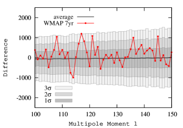
Figure 1: Differences between the WMAP angular power spectrum $C_{\ell}^{\rm WMAP}$ and the power spectrum of the $\Lambda$CDM model $C_{\ell}^{\rm\Lambda CDM}$ (red line). The boxes represent the variance of $1,2,3\sigma$ at each $\ell$ estimated from the 3,0000 simulations. The black line represents the average value of residuals between $C_{\ell}^{j}$’s and $C_{\ell}^{\rm\Lambda CDM}$.

III.2 significance of the structure

In the multipole region of $\ell=100$ – $150$, the distributions of the $C_{\ell}$’s are well approximated by the Gaussian one. In that case the probability that the $C_{\ell}$ is within $1\sigma$ and $2\sigma$ should correspond to about 68.3% and 95.5%, respectively. In our analysis, there are 51 data points because we focus only between $\ell=100$ – $150$, and the expected number of data over $1\sigma$ or $2\sigma$ is estimated as 16.2 or 2.3 points, respectively. Thus, it is natural that some data points deviate from the theoretical curve to this extent. However, from Fig. 1, we find that 19 and 7 points of data are over $1\sigma$ and $2\sigma$ levels, respectively. That indicates the $C_{\ell}^{\rm WMAP}$ somewhat deviates from the standard Gaussian distribution more than expected.

We roughly estimate the probability $P$ as a function of $N_{2\sigma}$ and $N_{1\sigma\mbox{-}2\sigma}$ which are the numbers of realization that exceeds $2\sigma$ and lies between 1$\sigma$ and 2$\sigma$, respectively, assuming the realization follows the Gaussian distribution. We show the result as contours in Figure. 2. In the figure the red, green and blue lines represent $1\sigma$, $2\sigma$ and $3\sigma$, respectively. From the figure, we can see that the peak is at the expected value ($N_{1\sigma\mbox{-}2\sigma}$,  $N_{2\sigma}$) = (13.9,  2.3), and the probability decreases with distance away from the expected value. The yellow point represents the value from the WMAP data; ($N_{1\sigma\mbox{-}2\sigma}$,  $N_{2\sigma}$) = (12,  7). It lies at the location between 2.5–$3\sigma$, which is consistent with the result of Ichiki and Nagata (2009). Therefore, we can understand that the fine structures at the range of $\ell=100$–150 of the angular power spectrum which are observed by WMAP team seem a rare event, if these structures are generated only by the noise and the cosmic variance effects.

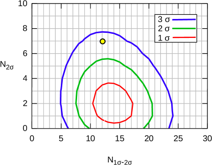
Figure 2: Contours of equal probabilities as a function of $N_{1\sigma\mbox{-}2\sigma}$ and $N_{2\sigma}$. The red, green and blue lines correspond to $1\sigma$, $2\sigma$ and $3\sigma$, respectively. The (yellow) point represents the WMAP data.

If the structures were not related to the noise nor cosmic variance, the other possibilities would be foreground effects and/or real cosmological signal. From the next section, we examine frequency and direction dependences of the fine structures in order to investigate whether the structures come from cosmological or astronomical phenomena.

IV Frequency dependence

If any astronomical phenomena such as syncrotron emission, dust emission and radio galaxies infiltrate the CMB temperature fluctuation data and create the fine structures, we expect that they have a characteristic frequency dependence. Therefore, we estimate the angular power spectra for three different frequency bands, namely Q, V and W bands. We find that the shapes of the fine structures at each frequency band are very similar to each other and to the all sky one (Fig. 1). Thus it is improbable that the fine structures originate from astrophysical phenomena nor objects, because they will have different frequency dependences from the CMB blackbody spectrum.

V Analysis with the partial skies

In this section, we look into the differences in the angular power spectra for different sky directions. For this purpose we prepare four masks, namely the North West mask ($0\leq\phi\leq\pi$, $0\leq\theta\leq\pi/2$), the North East mask ($\pi\leq\phi\leq 2\pi,\,0\leq\theta\leq\pi/2$), the South West mask ($0\leq\phi\leq\pi,\,\pi/2\leq\theta\leq\pi$) and the South East mask ($\pi\leq\phi\leq 2\pi,\,\pi/2\leq\theta\leq\pi$). We show these masks in Fig. 3.

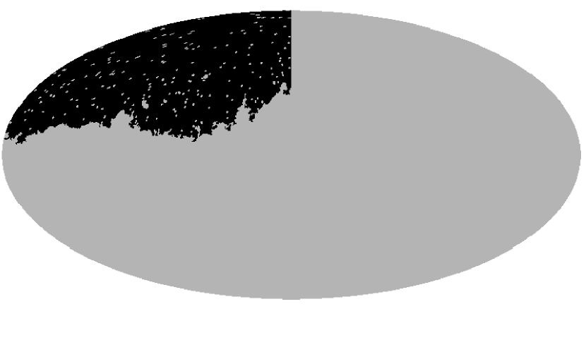
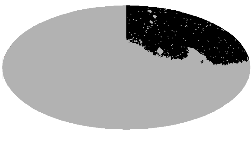
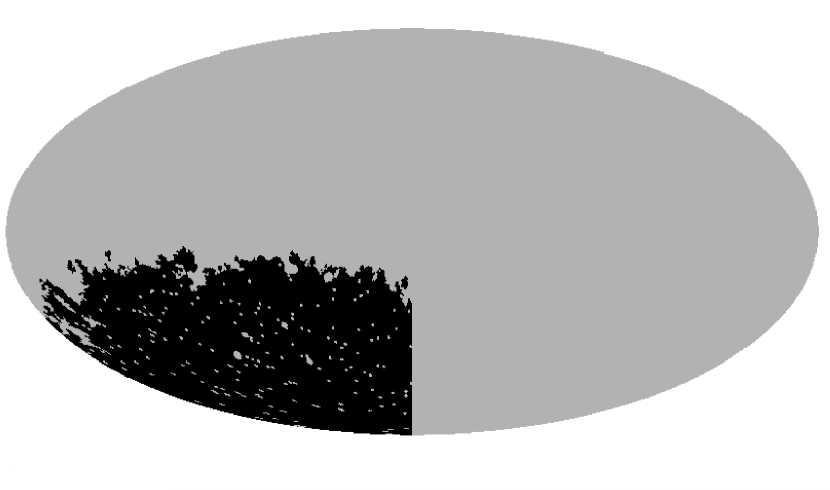
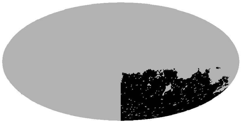
Figure 3: Masks of the partial skies used in our analysis in the galactic coordinate. The left top panel refers to North West mask, the right top panel to North East mask, the left bottom panel to South West mask and, finally, the right bottom to South East mask.

Using the masks, first let us calculate the gap between the angular power spectra of the simulated maps and that of the observed map by WMAP for the partial skies. Further, we compare the partial sky maps with each other, in order to see the dependence of the angular power spectrum on the sky directions. However, some difficulties arise when analyzing the CMB map with a partial sky mask. Because a mask narrows down the effective area of the spherical surface, effective information is reduced. Furthermore, if a mask has a sharp cutoff at the boundary, it will lead a truncated correlation function. Computing the angular power spectrum from the truncated correlation function causes spurious oscillations inherent to the Fourier transformation, which is known as the ”Gibbs phenomenon”. However, these oscillations have nothing to do with the anisotropy of the CMB nor the fine structures, and they can be removed by apodization and binning techniques as we describe below.

In the next two subsections, we review these techniques that we used in order to lighten and avoid these nuisance effects, and in the final subsection, we show the direction dependence of the CMB angular power spectrum.

V.1 Apodization

In fact, we find that spurious oscillatory structure in the angular power spectrum that arises when the masks are used is caused by the large amplitude oscillations in the two point correlation function at large angular scales. The oscillations are caused by the statistical errors. Indeed, if we use a map with a maximal angular size $\theta_{\rm max}$, nothing can be known about the correlation function for $\theta\gtrsim\theta_{\rm max}$. However, simply truncating the correlation function at $\theta=\theta_{\rm max}$ does not help the situation as we mentioned above. Instead, the technique uses an appropriate function, called the ”apodization function” $F(\theta)$, and multiplies it with the correlation function $\xi(\theta)$ for the product to go to zero smoothly Szapudi et al. (2000); Chon et al. (2004). Angular power spectrum is then given by

$$C^{\rm apd}_{\ell}=2\pi\int_{\theta=0}^{\theta_{\rm max}}\,\sin\theta d\theta\,\,\xi(\theta)F(\theta)P_{\ell}(\cos\theta)~{},$$ (8)

where $\theta_{\rm max}$ is the maximum angle set by the mask. We can adopt any function as an apodization function which takes $F(\theta)=1$ at $\theta=0$ and decreases as $\theta$ increases. The Gaussian type $F_{\rm G}(\theta)$ and Cosine type $F_{\rm C}(\theta)$ are often adopted, and they are defined as

$$F_{\rm G}(\theta) = \exp\left[-\frac{\theta^{2}}{2(\sqrt{8\ln 2}\,\sigma_{\rm apd})^{2}}\right],$$ (9)

$$F_{\rm C}(\theta) = \frac{1}{2}\left[1+\cos\left(\pi\frac{\theta}{\sigma_{\rm apd}}\right)\right]~{},$$ (10)

where $\sigma_{\rm apd}=\pi\theta_{\rm apd}/180^{\circ}$ and $\theta_{\rm apd}$ represents the angle in degree where the apodization function becomes close to zero. Typical value of $\theta_{\rm apd}$ should be close to the cut off angle $\theta_{\rm max}$.

We calculate the angular power spectrum with apodization and show the results in Fig. 4. In the upper panel of the figure, in the case of $\theta_{\rm max}=100^{\circ}$ when the North West mask is used, the oscillatory feature with a large amplitude can be seen on the angular power spectrum, because we truncate the integral in Eq.(7) at $\theta=100^{\circ}$. In the case of $\theta=180^{\circ}$ when KQ75 mask is used, on the other hand, the oscillation is suppressed because $\xi$ decreases as $\theta\to 180^{\circ}$. The lower panel shows the results with apodization using the Gaussian and Cosine type functions, setting $\theta_{\rm apd}$ to $100^{\circ}$. As is shown in the lower panel, the resultant power spectra become smooth compared to the case without apodization (see the red line in the upper panel). Also it is noted that the shape of the apodized spectra is similar to the power spectrum of the full sky ($\theta_{\rm max}=180^{\circ}$; the black line), though small scale oscillations have smoothed out. This is a bad news because we are interested in the fine structures.

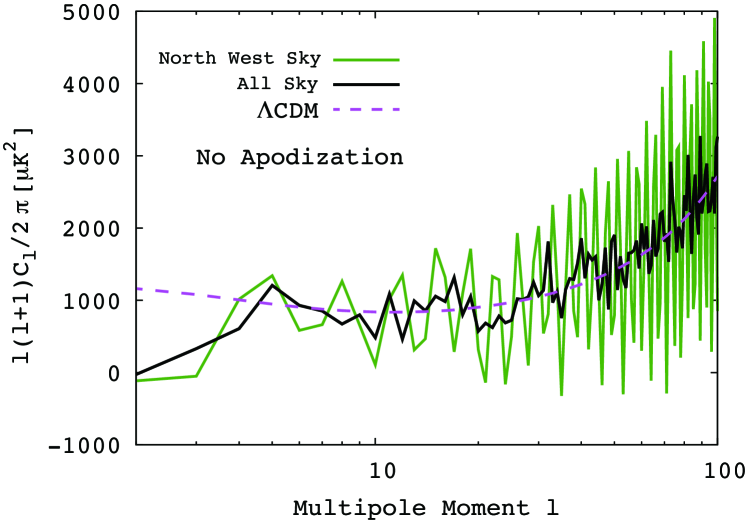
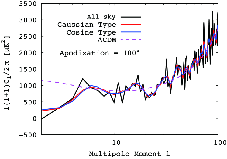
Figure 4: Angular power spectra estimated from two-point correlation functions. In the upper panel, the red line represents the power with the North West mask and with $\theta_{\rm max}=100^{\circ}$ in Eq.(8), (which corresponds to a truncated correlation function) and the black line the case with KQ75 mask. The theoretical curve of the $\Lambda$CDM model is also shown (the magenta line). When we naively analyze the partial sky, the large spurious oscillations arise on the angular power spectrum. In the lower panel, we show the cases with apodization, with $\theta_{\rm apd}=100^{\circ}$. The black and magenta lines are same as in the upper panel. The red and blue lines represent the apodized $C_{\ell}$ with Gaussian and Cosine types, respectively. For both cases, the North West mask is used. The suppression of the spurious oscillations is clearly seen due to the apodization function.

Figure 5: The apodization functions $F(\phi)$ of Cosine type (solid) and Gaussian type (dashed). The $\theta_{\rm apd}$ parameters are fixed as they suppress enough the spurious oscillations ($\theta^{\rm cos}_{\rm apd}=140^{\circ}$, and $\theta_{\rm apd}^{\rm Gauss}=100^{\circ}$). These lines indicate that the information lost is heavier for the case of Gaussian type apodization than that of Cosine type.

As we take $\theta_{\rm apd}$ smaller, more significant the smoothing effect for the fine structures in the angular power spectrum becomes. Therefore we should take the angle $\theta_{\rm apd}$ as large as possible to keep the fine structures. The maximum apodization angles $\theta_{\rm apd}$ for our masks with a sufficient suppression of the spurious oscillations are found to be $140^{\circ}$ and $100^{\circ}$ for the Cosine and Gaussian types, respectively. In Fig. 5 we depict the apodization functions with those $\theta_{\rm apd}$. From the figure, we can notice that the Gaussian type reduces the information in the two-point correlation function at large angles more than the Cosine one. In this work, we should keep the information as much as possible, because we focus on the fine structures. Therefore, we use the Cosine type apodization function in the following analysis. In this case, the structure at $\ell=100$–150 can survive the apodization because the amplitude of the apodization function at this scale is over 0.99.

As the loss of information about high frequency structure in the angular power spectrum is significant, components of $C_{\ell}$ become correlated with each other. This effect and coping technique are discussed in the next subsection.

V.2 Binned angular power spectrum

In the previous subsection, we see the apodization technique suppresses the high frequency oscillations. However, this technique is unavoidably accompanied with the loss of information. The loss appears as correlations between two different multipole moments. In order to see the degree of the correlations, let us calculate the covariance matrix ${\cal C}_{\ell\ell^{\prime}}$,

$${\cal C}_{\ell\ell^{\prime}}\equiv\frac{1}{\bar{C}_{\ell}^{2}}\frac{1}{N}\sum_{i=1}^{N}\left(C_{\ell}^{i}-\bar{C}_{\ell}\right)\left(C_{\ell^{\prime}}^{i}-\bar{C}_{\ell^{\prime}}\right)~{},$$ (11)

where

$$\bar{C}_{\ell}=\frac{1}{N}\sum_{i=1}^{N}C_{\ell}^{i}~{}.$$ (12)

Here, $C_{\ell}^{i}$ is the estimated angular power spectrum from the $i$th Monte Carlo simulation sky, N is the total number of the samples. From this matrix, we can estimate the strength of correlations between each multipole moment. If there are no correlations, which means the $C_{\ell}$ can be estimated independently, the covariance matrix should be diagonal.

On the contrary, the covariance matrix has off-diagonal elements if the $C_{\ell}$ depends on another multipole moment component $C_{\ell^{\prime}}$. The correlations between the $C_{\ell}$’s are caused by the mask. If a mask is applied on the CMB sky, the estimated angular power spectrum is given by a convolution between the power spectra of the mask and the true temperature anisotropies that we want to estimate. The convolution generates correlations between the multipoles of $\Delta\ell\simeq$ 2–3, which makes it complicated to estimate the statistical significance of the angular power spectrum. A simple way to obtain independent observable is to bin the angular power spectrum with the comparable bin width.

The covariance matrices of the angular power spectrum with KQ75 mask are depicted in Fig. 6. The upper panel in the figure shows the matrix for the case without apodization. Each component of this matrix is practically vanishing except for the diagonal ones. This result indicates that the correlations caused by the KQ75 mask are not significant at the multipole region of $100\leq\ell\leq 150$. This is because the condition that $\Delta\ell\geq\frac{\pi}{\theta_{\rm max}}\sim 1$ can still be satisfied with the mask, where $\theta_{\rm max}$ is the maximum separation angle in the pixel domain. On the other hand, in the middle panel, we use the KQ75 mask with apodization. In this case, the components around diagonal elements do not vanish. This manifests the information loss due to apodization, though the variances (diagonal elements) become smaller values.

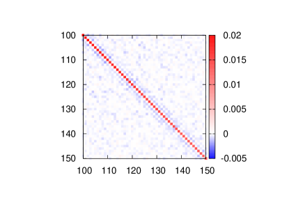
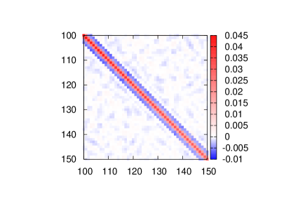
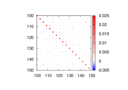
Figure 6: Covariance matrices of angular power spectra ${\cal C}_{\ell\ell^{\prime}}$. The upper and middle panels show the covariance matrices without apodization and with Cosine type apodization, respectively. Non-zero off-diagonal components indicate the presence of correlation between $\ell$ and $\ell^{\prime}$. In the bottom panel we show the covariance matrix of the binned angular power spectrum. We can see that the correlation between components becomes weak.

The correlations appear only between the neighboring multipoles. To reduce the correlations we should gather the neighboring components in one component, namely, bin the data. The contributions from the neighboring modes $\ell^{\prime}$ to the pivot scale $\ell$ are about 50% ($\ell^{\prime}=\ell\pm 1$) and -10% ($\ell^{\prime}=\ell\pm 2,\ell\pm 3$), which is shown in the middle panel of Fig. 6. We find that a binning with $\Delta\ell=3$ is sufficient because the positive and negative correlations nicely compensate with each other to reduce the correlations between the binned data. In this case the number of data points reduces to 17 from 51, and this reduction could lead some information loss. The covariance matrix of this case is depicted in the lower panel of Fig. 6. Looking at this figure, we can see that the correlation becomes weak enough thanks to the binning. Then, each components can be considered approximately independent.

Although binning is useful to simplify the statistics, some information should be lost in the process, especially if there exist fine structures in the data. In the next subsection we show how the binning procedure affects the fine structures in multipole $\ell=100$–150 we are interested in.

We calculate the binned $C_{\ell}$’s and verify the fine structures using the same steps we followed in Sec. III. There are three ways to select the pivot scale for binning. We calculate the binned spectra with the three patterns $C_{\ell}^{\rm B}=\sum_{i=-1}^{1}C_{\ell+i}/3$ for case I ($\ell=99+3n$), case II ($\ell=100+3n$), and case III ($\ell=101+3n$) where $n=1,2,\cdots,17$. The results are shown in Fig. 7. The right panels represent the probability that the fine structures come from the noise and the cosmic variance effects, as we have shown in Fig. 2. The result slightly depends on the binning pattern, but in any cases the significance is above 2.5 $\sigma$. In the left panels of Fig. 7, we show the residuals between binned $C_{\ell}^{\rm WMAP}$ and $C_{\ell}^{\rm\Lambda CDM}$ as red lines. The black line is the average of $C_{\ell}$ with the 3,000 simulations. The dispersion of the simulation data is also shown as the grey boxes. We can still see the oscillatory feature that is found in the case without binning for all sky, and some points are over 1$\sigma$ box or 2$\sigma$ box. The numbers of data points above 1 or 2 $\sigma$ are larger than expected from Gaussian distribution for all cases. These results indicate that the fine structures can survive even if we apodize and bin the angular power spectrum.

We consider these three power spectra as the fiducial binned power spectra of WMAP for the full sky. To figure out the origin of the fine structures we compare them with the spectra from the partial skies obtained with the same apodization function and binning, as we shall show in the next section.

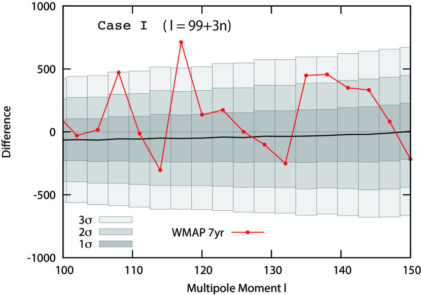
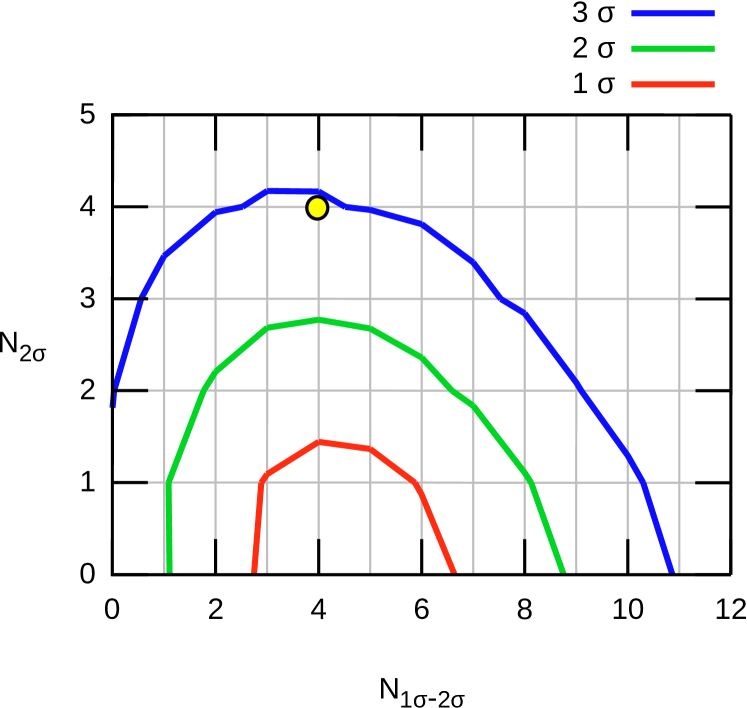
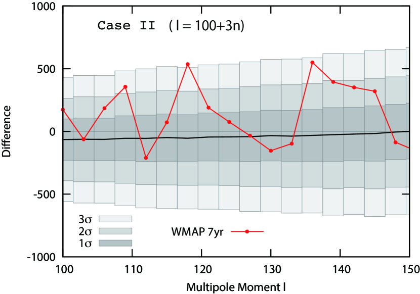
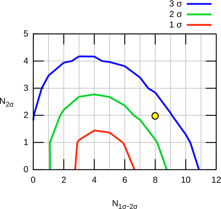
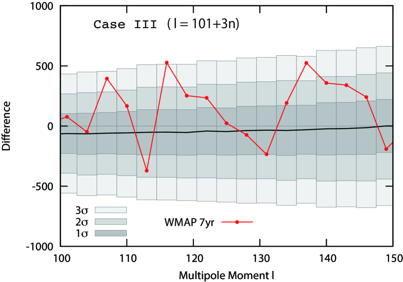
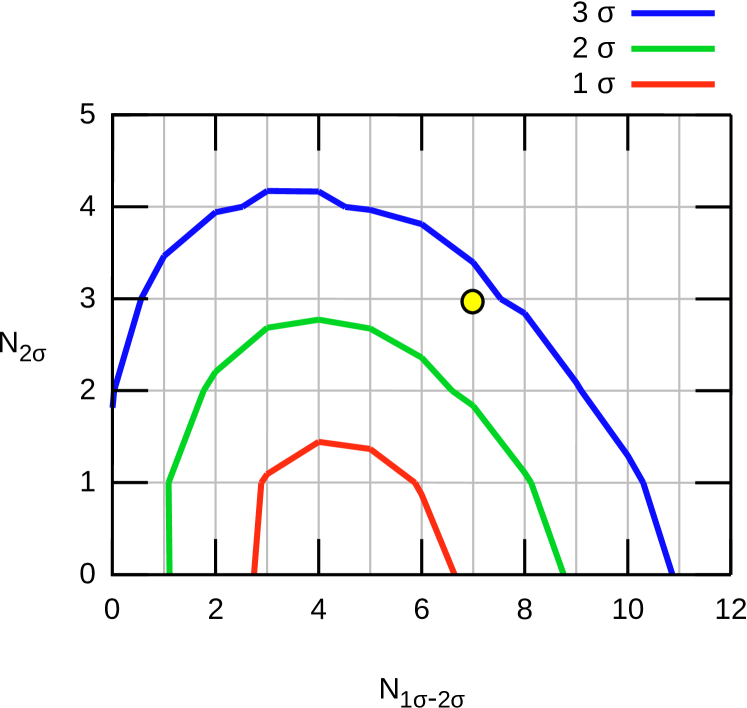
Figure 7: Left: Differences in the binned spectra between the predicted angular power spectrum from the $\Lambda$CDM model and the WMAP power spectrum with apodization function ($\theta_{\rm max}=140^{\circ}$. The black line represents the average value of the 3,000 mock data. The deviation from zero manifests the $\chi^{2}$-like distribution of the angular power spectrum. The boxes are the variances estimated from the mock data, as indicated in the figure. Right: The probability contours assuming Gaussian distribution for each binned power with no correlation and the WMAP data, as in Fig. 2.

V.3 The angular power spectrum with partial sky

In the previous sections we have seen that the apodization and binning can successfully remove the spurious oscillations and the correlations between multipoles due to the partial sky mask. Here we apply the same technique to the four different partial skies and see whether there exists the directional dependence of the fine structures in the angular power spectrum. In the following discussion, we separate the structures into two characteristic structures. First one is the oscillatory structure around $\ell=100$ – $120$. The two peaks have a significant deviation from the smooth spectrum at around 3$\sigma$. The other is the bump around $\ell=140$.

We show the results for the binning case I in the upper panel of Fig. 8. The primary effect of the partial sky masks can be seen in the error bars. The estimated error bars depend on the number of available modes $N$ as $1/\sqrt{N}$. In our analysis the effective sky coverage for the partial sky becomes about one-quarter compared to the all sky map. Therefore the error bar should be twice of the case of the all sky (Fig. 7) and we can confirm this fact from the figure.

We find a distinct anisotropic structure which is above 3$\sigma$ error bar at $\ell=138$ in the South East area (bottom right panel of Fig. 8), which is highlighted by a double circle in figure. Also, the histogram of the difference between $\Lambda$CDM and the simulated data set at $\ell=138$ is shown in the lower panel of Fig. 8 for each direction. The vertical red lines show the differences of the power between the $\Lambda$CDM and the observed one by WMAP. The anisotropic structure in the South East can be seen in the other binning cases, as in Figs. 9, and 10.

The peculiarity of South East area as a whole at the multipole range of $100\leq\ell\leq 150$ can be quantified with the value of $\chi^{2}$, defined by

$$\chi^{2}=\sum_{i=1}^{17}\left(C_{\ell}^{\rm B}-\bar{C}_{\ell}^{\rm B}\right){\cal C}_{\ell\ell^{\prime}}^{{\rm B}^{-1}}\left(C_{\ell^{\prime}}^{\rm B}-\bar{C}_{\ell^{\prime}}^{\rm B}\right)/\bar{C}^{\rm B}_{\ell}\bar{C}^{\rm B}_{\ell^{\prime}}~{},$$ (13)

where ${\cal C}_{\ell\ell^{\prime}}^{{\rm B}^{-1}}$ is the inverse of the covariance matrix of the binned angular power spectrum. We show the probability distribution function of $\chi^{2}$ , written by

$$F(\chi^{2};n=17)=\frac{(\chi^{2})^{n/2-1}}{2^{n/2}\Gamma(\frac{n}{2})}e^{-\chi^{2}/2}~{},$$ (14)

and the values of $\chi^{2}$ for the four partial skies in Fig. 11. The value of $\chi^{2}$ away from the peak position indicates the overall deviation of the observed angular power spectrum from the average value of the mock power spectrum. From this figure, the South East area has especially peculiar $\chi^{2}$ value. The probability that the $\chi^{2}$ takes larger value than the South East area by chance can be estimated as 1.50 (case I), 1.56 (case II), 8.70 (case III) %.

These results may suggest a possibility of existence of characteristic features only at South East area. The structure which comes from cosmological origin can be assumed to be isotropic, and therefore this anisotropic structure around $\ell\approx 138$ might be attributed to some astronomical origin, which have the scale about $0.6^{\circ}$. It may be interesting to note that there has been a report about a power spectrum anomaly around the third acoustic peak at the same sky direction Ko et al. (2011), although the authors argued that the origin could be the WMAP instrumental noise because the third acoustic peak is located at the limit of the WMAP angular resolution.

The oscillatory feature (peak and dip) that is found in the all sky analysis around $\ell=100$ – $120$, on the other hand, can be found clearly in the North West area, and also found at all the other directions regardless of the binning cases. Thus, the oscillation seems to be caused by some cosmological origin, not the astrophysical one.

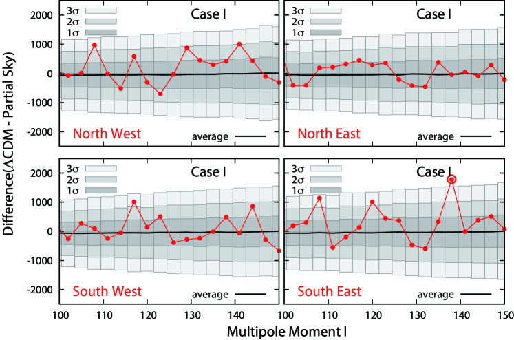
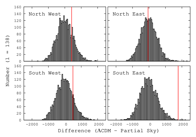
Figure 8: Upper panels: The same as the left panels in Fig. 7, but for the partial skies with binning case I. Lower panels: The histograms of differences between the power spectrum of $\Lambda$CDM and those from the 3,000 mock data at $\ell=138$. The red line corresponds to the data point of WMAP. The peculiarity of South East sky is clearly shown.

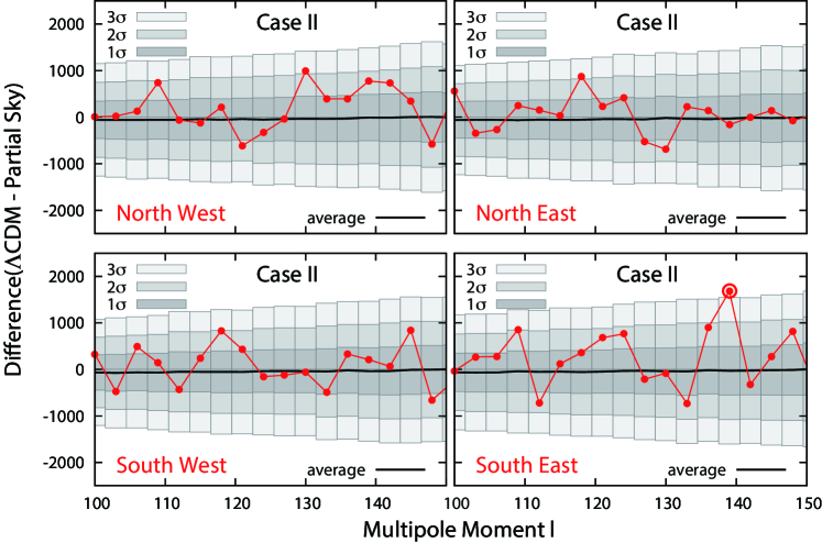
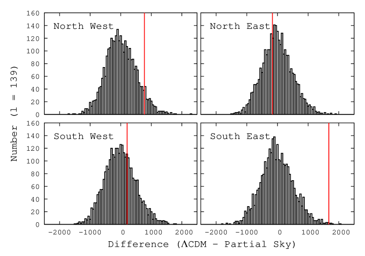
Figure 9: Same as Fig. 8 but for the binning case II and $\ell=139$ (lower panel).

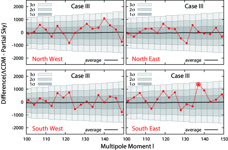
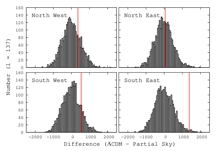
Figure 10: Same as Fig. 8 but for the binning case III and $\ell=137$ (lower panel).

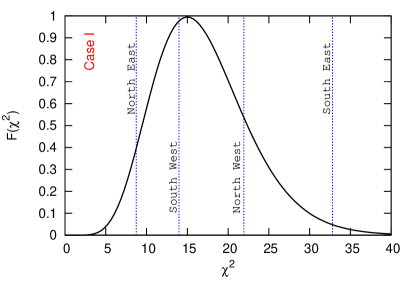
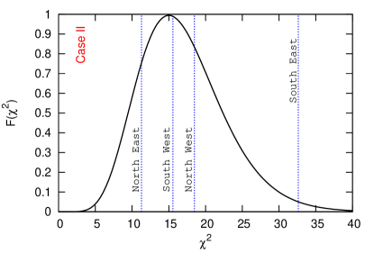
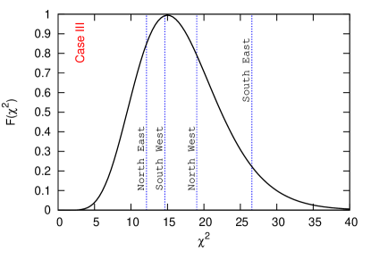
Figure 11: The $\chi^{2}$ distribution derived from the 3,000 simulations and the $\chi^{2}$ values of WMAP at each direction for each binning case.

VI Summary

In this work we have re-examined the temperature angular power spectrum of the cosmic microwave background (CMB) at three frequency bands and for four restricted sky directions, in order to explore the origin of the fine structures in the power at the multipole range of $100\leq\ell\leq 150$.

We prepared 3,000 mock sky maps of CMB temperature fluctuations with anisotropic instrumental WMAP noise, and verified the noise and cosmic variance effect on the fine structures of the WMAP data. By comparing the angular power spectra from each mock data with the real data by the WMAP, we found that the probability of the fine structures to be realized by chance is about 2 - 3$\sigma$. We checked whether the fine structures of the power spectrum depend on the Q, U, and V band maps, and found no evidence for the frequency dependence.

In contrast, we obtained some interesting suggestions from the angular power spectra derived from the partial skies. We found that the characteristic bump around $\ell=130$ – $140$ seen in the all sky angular power spectrum is solely attributed to the anomalous power at the South East area. We have already known the existence of the cold spot as one of the anisotropy structures in South East area Cruz et al. (2007); Inoue and Silk (2006). We have doubt if the cold spot will affect at $\ell=140$ as a substrucure, thought the cold spot is few degree scale. However, we confirm that this effect is too tiny to generate characteristic structures at $\ell=140$. This result may indicate the existence of unknown peculiar structure in that area as the origin of the fine structure. The fine oscillating structures found around $\ell=100$ – $120$, on the other hand, have no significant directional dependences, suggesting that the oscillations come from some cosmological origin.

If the observed feature is not a statistical fluctuation but has a primordial origin, a straight but important test is to look into the polarization of the CMB and/or the distribution of the large scale structure, because they should show the same characteristic structure in their power spectra. The coming data by PLANCK Planck Collaboration et al. (2011) and future galaxy survey such as the Large Synoptic Survey Telescope LSST Science Collaborations et al. (2009) can be used for the cross check and to accept (or reject) the feature with high significance.