Identification of members in the central and outer regions of galaxy clusters

Abstract

The caustic technique measures the mass of galaxy clusters in both their virial and infall regions and, as a byproduct, yields the list of cluster galaxy members. Here we use $100$ galaxy clusters with mass $M_{200}\geq 10^{14}h^{-1}M_{\odot}$ extracted from a cosmological $N$-body simulation of a $\Lambda$CDM universe to test the ability of the caustic technique to identify the cluster galaxy members. We identify the true three-dimensional members as the gravitationally bound galaxies. The caustic technique uses the caustic location in the redshift diagram to separate the cluster members from the interlopers. We apply the technique to mock catalogs containing 1000 galaxies in the field of view of $12h^{-1}$ Mpc on a side at the cluster location. On average, this sample size roughly corresponds to 180 real galaxy members within $3r_{200}$, similar to recent redshift surveys of cluster regions. The caustic technique yields a completeness, the fraction of identified true members, $f_{c}=0.95\pm 0.03$ within $3r_{200}$. The contamination, the fraction of interlopers in the observed catalog of members, increases from $f_{i}=0.020^{+0.046}_{-0.015}$ at $r_{200}$ to $f_{i}=0.08^{+0.11}_{-0.05}$ at $3r_{200}$. No other technique for the identification of the members of a galaxy cluster provides such large completeness and small contamination at these large radii. The caustic technique assumes spherical symmetry and the asphericity of the cluster is responsible for most of the spread of the completeness and the contamination. By applying the technique to an approximately spherical system obtained by stacking the individual clusters, the spreads decrease by at least a factor of two. We finally estimate the cluster mass within $3r_{200}$ after removing the interlopers: for individual clusters, the mass estimated with the virial theorem is unbiased and within 30% of the actual mass; this spread decreases to less than 10% for the spherically symmetric stacked cluster.

1. Introduction

Galaxy clusters provide crucial information to our understanding of the large-scale cosmic structure and to constrain cosmological models. They populate the high-mass tail of the mass function of virialized galaxy systems; their abundance and redshift distribution depend on the average density of the universe and the normalization of the power spectrum of the initial density perturbations (e.g., Voit 2005; Diaferio et al. 2008; Borgani 2008). Clusters are a hostile environment to galaxies and are thus also a unique tool to investigate the connection between environment and galaxy properties (e.g., Domínguez et al. 2001; Martínez et al. 2008; Skibba et al. 2009; Huertas-Company et al. 2009).

Separating the galaxies that do actually belong to the cluster from the interlopers -the galaxies that happen to lie in the field of view but are not dynamically linked to the cluster- is crucial to derive accurate estimates of the cluster properties, including its mass (Perea et al. 1990), or the color and star formation gradients of its galaxy population (Diaferio et al. 2001a).

Interloper rejection techniques are numerous and their sophistication has progressively increased over the years, thanks to the increased quality and richness of the observational data: over the last decade, the handful of clusters with tens of measured redshifts within $\sim 1-2$$h^{-1}$Mpc of the cluster center has increased by at least a factor of 10 (e.g., Rines et al. 2003; Rines & Diaferio 2006; Geller et al. 2011).

Early observations of galaxy clusters do not usually extend into the outer regions of the system. Early interloper rejection techniques identify galaxy members solely on the basis of their redshift separation from the cluster center. The gravitational potential well can however become substantially shallower at increasing radius and the combination of velocity and radial distance is now an essential ingredient for the identification of galaxy members in samples that extend to the cluster virial radius and beyond.

The caustic technique (Diaferio & Geller 1997; Diaferio 1999, 2009; Serra et al. 2011) identifies the escape velocity profile of galaxy clusters from their center to radii as large as $3r_{200}$, where $r_{200}$ is the radius of the sphere whose average density is 200 times the critical density of the Universe. The technique was thus applied to estimate the gravitational potential well and the mass profiles of galaxy clusters to radii that extend to the cluster infall region (see reviews in Diaferio 2009 and Serra et al. 2011). Where the cluster is in the appropriate redshift range for weak lensing mass estimation and a comparison is thus possible, caustic and lensing masses agree within 30% at the virial radius (Diaferio et al 2005, Geller et al 2013), whereas at smaller and larger radii the two mass estimates show a systematic offset of at most 50% and 20% respectively (Geller et al. 2013).

Because the technique measures the escape velocity profile, a byproduct of the caustic procedure is the identification of interlopers. Compared to other interloper rejection algorithms the caustic technique has two major advantages: (1) it does not require the system to be in dynamical equilibrium and (2) it does not rely on the derivation of the cluster mass profile to remove interlopers. These advantages enable the technique to identify interlopers both in the central and outer regions of clusters, where other techniques can not be applied. The caustic technique assumes spherical symmetry, an assumption that is common to most methods. In addition, when used as a mass estimator method, the caustic technique returns correct mass estimates if clusters form by hierarchical clustering and thus they have the internal kinematical and dynamical properties, including the shape of the velocity anisotropy profile, that clusters generally have in these models.

The caustic technique as an interloper rejection algorithm, or some simplified versions of it, was applied to real clusters to investigate the dependence of galaxy properties on environment (e.g., Rines et al. 2000, 2004, 2005; Mahajan & Raychaudhury 2009; Hernández-Fernández et al. 2012; Hwang et al. 2012), and to provide robust estimates of the cluster velocity dispersion and mass (e.g., Benatov et al. 2006; Lemze et al. 2009; Zhang et al. 2011, 2012).

Thanks to the approximate self-similarity of self-gravitating systems, the technique can also be applied to reject stellar interlopers in galaxies: Brown et al. (2010) used the caustic method results to estimate the velocity dispersion profile of the stars in the Milky Way halo, and Serra et al. (2010) demonstrated that a proper stellar interloper rejection alleviates the tension between the internal velocity dispersion profiles of the Milky Way dwarf satellites and the expectations of Modified Newtonian Dynamics. Yegorova et al. (2011) also probed the dark matter distribution in the outer regions of disk galaxies by identifying their satellites with the caustic technique.

Despite this extensive application, the caustic technique has never been exhaustively explored as a method to identify interlopers. Here, we provide a thorough analysis of its performance and of its random and systematic errors. In Section 2 we briefly describe the caustic technique, whereas in Section 3 we present the mock cluster catalogs. In Section 4 we discuss the technique performance. We finally investigate the impact of our interloper rejection on the cluster mass estimates in Section 5. We compare the performance of our method with other rejection techniques in Section 6. Conclusions are presented in Section 7.

2. The Caustic Technique

In hierarchical clustering, clusters of galaxies form by the aggregation of smaller systems. The accretion is not purely radial (e.g., White et al. 2010), because galaxies within the falling clumps have velocities with a substantial non-radial component. Therefore, the galaxy velocities are set by the local gravitational potential more than by the radial infall expected in the spherical collapse model (Diaferio & Geller 1997).

When observed in the redshift diagram -the plane of the line-of-sight velocity $v$ of the galaxies in the cluster rest frame versus their projected distance $r$ from the cluster center- the cluster members populate a region with a trumpet shape approximately symmetric along the $r$ axis (Kaiser 1987; Regös & Geller 1989; van Haarlem & van de Weygaert 1993). The caustics define the boundaries of this region whose amplitude ${\cal A}(r)$ decreases with increasing $r$. Diaferio & Geller (1997) demonstrate that ${\cal A}(r)$ is a combination of the profile of the escape velocity from the cluster and the profile of the velocity anisotropy parameter $\beta(r)=1-(\langle v^{2}_{\theta}\rangle+\langle v^{2}_{\phi}\rangle)/2\langle v^{2}_{r}\rangle$, where $v_{\theta}$, $v_{\phi}$, and $v_{r}$ are the longitudinal, azimuthal and radial components of the velocity ${\mathbf{v}}$ of a galaxy, respectively, and the brackets indicate an average over the velocities of the galaxies in the volume $\mbox{d}^{3}{\bf r}$ centered on position ${\bf r}$.

In a spherically symmetric system, the average square of the velocity of the system members at radius $r$ is $\langle v^{2}\rangle=\langle v^{2}_{\rm los}\rangle g(\beta)$ where $\langle v^{2}_{\rm los}\rangle$ is the component of the line-of-sight velocity and

$$g(\beta)={3-2\beta(r)\over 1-\beta(r)}\;.$$ (1)

For the escape velocity at radius $r$, we have $\langle v_{\rm esc}^{2}(r)\rangle=-2\phi(r)$, where $\phi(r)$ is the gravitational potential. If the amplitude ${\cal A}(r)$ measures the average component along the line of sight of the escape velocity at radius $r$, namely ${\cal A}^{2}(r)=\langle v^{2}_{\rm esc,los}\rangle$, we obtain the relation

$$-2\phi(r)={\cal A}^{2}(r)g(\beta)\equiv\phi_{\beta}(r)g(\beta)\;.$$ (2)

This equation shows the dynamical information contained in the observable caustic amplitude ${\cal A}(r)$. Being a combination of the gravitational potential profile and the function $g(\beta)$, ${\cal A}(r)$ can provide the estimate of both the escape velocity profile from the cluster and the mass profile of the cluster (Diaferio & Geller 1997; Diaferio 1999). We emphasize that the entire argument outlined above holds regardless of the stability of the system.

To measure ${\cal A}(r)$ we need to locate the caustics in the redshift diagram. The technique consists of three major steps: (1) the construction of a binary tree based on the projected galaxy pairwise energy; (2) the determination of a threshold to cut the binary tree; (3) the identification of the cluster center to obtain the redshift diagram and determine the galaxy number density on this diagram.

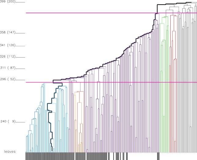
Figure 1.— Dendrogram representation of the binary tree of a random subsample of 200 particles in the field of view of a simulated cluster. The particles are the leaves of the tree at the bottom of the plot. The particles within $3r_{200}$ in real space are highlighted in black. The thick path highlights the main branch of the tree. The horizontal lines show the levels at the two nodes $x_{1}$ (upper line) and $x_{2}$ (lower line) that limit the $\sigma$ plateau shown in Figure 3. The upper node $x_{1}$ is the threshold where the tree is cut and the main group is the structure hanging from this node. Only as a guide, some nodes are labeled on the left-hand side, with their number of associated particles, the descendants, in brackets.

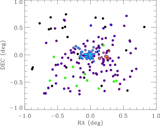
Figure 2.— Celestial coordinates of the subsample of 200 particles in the field of view of the simulated cluster whose binary tree is shown in Figure 1. The color code is the same as in Figure 1.

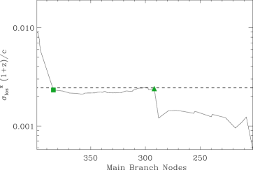
Figure 3.— Velocity dispersion of the leaves of each node along the main branch of the binary tree shown in Figure 1. The square and the triangle show the nodes $x_{1}$ and $x_{2}$ respectively. The curve between $x_{1}$ and $x_{2}$ is the $\sigma$ plateau. The dashed line shows the line-of-sight velocity dispersion of the particles within the sphere of radius $3r_{200}$.

At the first step, all the galaxies are arranged in a binary tree according to their pairwise binding energy

$$E_{ij}=-G{m_{i}m_{j}\over R_{p}}+{1\over 2}{m_{i}m_{j}\over m_{i}+m_{j}}\Pi^{2}\;,$$ (3)

where $R_{p}$ is the pair projected separation, $\Pi$ is the line-of-sight velocity difference and $m_{i}=m_{j}=10^{12}h^{-1}$ M_⊙ are the two galaxy masses assumed to be constant.

The binary tree is built as follows: (i) initially each galaxy is a group $g_{\alpha}$; (ii) the binding energy $E_{\alpha\beta}={\rm min}\{E_{ij}\}$, where $E_{ij}$ is the binding energy between the galaxy $i\in g_{\alpha}$ and the galaxy $j\in g_{\beta}$, is associated with each group pair $g_{\alpha},g_{\beta}$; (iii) the two groups with the smallest binding energy $E_{\alpha\beta}$ are replaced with a single group $g_{\gamma}$ and the total number of groups is decreased by one; (iv) the procedure is repeated from step (ii) until only one group is left. Figure 1 shows the binary tree of a random sample of 200 particles extracted from a simulated halo selected from the $N$-body simulation described in the next section, whereas Figure 2 shows the celestial coordinates of the same particles with the same color code as in Figure 1.

The second step of the caustic technique procedure is the threshold choice. The tree arranges the galaxies in potentially distinct groups; however, to get effectively distinct groups and to specifically define the set of candidate members, we need to cut the tree at some level. This level sets the node from which the candidate members hang. All these candidate members do not necessarily coincide with the optimal members that are determined by the caustic location. Below we will extensively illustrate the reason for this distinction between candidate and optimal members.

In order to choose the threshold to cut the binary tree, we identify the main branch as the branch that emerges from the root and contains the nodes from which, at each level, the largest number of galaxies (or leaves) hangs. The leaves hanging from each node $x$ of the main branch provide a velocity dispersion $\sigma_{\rm{los}}^{x}$. When walking along the main branch from the root to the leaves, $\sigma_{\rm{los}}^{x}$ rapidly decreases due to the progressive loss of galaxies that are most likely not associated with the cluster (Figure 3); then $\sigma_{\rm los}^{x}$ reaches a “$\sigma$ plateau” at some node $x_{1}$. Most of the galaxies hanging from this node are members; in fact, the system is nearly isothermal and the removal of the less bound galaxies does not affect the value of $\sigma_{\rm{los}}^{x}$. At some point of the walk along the main branch, the loss of the most bound galaxies, whose binding energy is very small, causes $\sigma_{\rm{los}}^{x}$ to drop again. This second rapid drop identifies the nodes $x_{2}$ which sets the limit of the $\sigma$ plateau. The first node $x_{1}$ closest to the root is the appropriate level for the identification of the system and we define the galaxies hanging from it the candidate members of the cluster. They determine the center of the system, its radius, and its line-of-sight velocity dispersion. These quantities are used to build the redshift diagram.

The third step of the procedure is the location of the caustics in the redshift diagram. The caustics are the curves satisfying the equation $f_{q}(r,v)=\kappa$. Here $f_{q}(r,v)$ is the galaxy number density in the redshift diagram, namely the plane $(r,v)$, and $\kappa$ is the root of the equation

$$\langle v_{\rm esc}^{2}\rangle_{\kappa,R}=4\langle v^{2}\rangle\;.$$ (4)

The function $\langle v_{\rm esc}^{2}\rangle_{\kappa,R}=\int_{0}^{R}{\cal A}_{\kappa}^{2}(r)\varphi(r)dr/\int_{0}^{R}\varphi(r)dr$ is the mean caustic amplitude within $R$, $\varphi(r)=\int f_{q}(r,v)dv$, $\langle v^{2}\rangle^{1/2}$ is the velocity dispersion of the candidate members, $R$ is their mean projected separation from the center, and $q$ is a smoothing parameter (see Diaferio & Geller 1997; Serra et al. 2011 for details).

Figure 4 shows the result of this procedure on the redshift diagram. We stress that the procedure to locate the caustics is independent of any assumption on the dynamical equilibrium of the system, of the shape of $g(\beta)$ and of the gravitational potential profile $\phi(r)$; this procedure actually measures the combination of $g(\beta)$ and $\phi(r)$ expressed by the caustic amplitude ${\cal A}(r)$ (Equation 2).

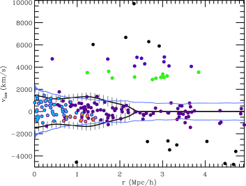
Figure 4.— Redshift diagram of the subsample of 200 particles in the field of view of the simulated cluster whose binary tree is shown in Figure 1. The black lines with error bars are the caustics located by the caustic technique. The cyan lines are the real caustics determined by the profiles of the escape velocity and the velocity anisotropy parameter derived by the three-dimensional information. The dots show the particles in the catalog and the color code is as in Figure 1.

3. Simulated clusters and mock catalogs

We use the synthetic galaxy clusters described in Serra et al. (2011) selected from the $N$-body simulation of Borgani et al. (2004). The simulation models a cubic volume of 192 $h^{-1}$ Mpc on a side of a flat $\Lambda$CDM model, with matter density $\Omega_{0}=0.3$, Hubble parameter $h=0.7$, normalization of the power spectrum $\sigma_{8}=0.8$ and baryon density $\Omega_{\rm b}=0.02h^{-2}$. The simulation contains $480^{3}$ dark matter particles with mass $m_{\rm DM}=4.6\times 10^{9}h^{-1}$ M_⊙ and, initially, $480^{3}$ gas particles with mass $m_{\rm gas}=6.9\times 10^{8}h^{-1}$ M_⊙. The simulation was run with GADGET-2 (Springel 2005). Further details of the simulations and the dark matter halo identification are given in Borgani et al. (2004). In the following, we limit our analysis to the gravitational dynamics of the dark matter distribution. In fact, both $N$-body simulations (e.g., Diaferio et al. 2001b; Gill et al. 2004; Diemand et al. 2004; Gill et al. 2005) and observations (e.g., Rines et al. 2008) indicate that any velocity bias between galaxies and dark matter is negligible.

We consider the 100 dark matter halos with mass $M(<r_{200})\equiv M_{200}\geq 10^{14}h^{-1}M_{\odot}$ at redshift $z=0$. We locate each halo at $(\alpha,\delta)=(6^{h},0^{\circ})$ and redshift $cz=32000$ km s^-1. We simulate the compilation of the redshift catalog of a galaxy cluster by projecting each halo along 10 random lines of sight. For each of these lines of sight, we choose two additional directions orthogonal to the first one and to each other. We end up with $3000$ mock redshift catalogs. Each catalog contains a random sample of $1000$ particles distributed within a rectangular parallelepiped centered on the cluster with a squared field of view of $12h^{-1}$ Mpc on a side and 192 $h^{-1}$ Mpc deep. With this number of particles in the field of view, we obtain a distribution of the number of particles within the sphere of radius $r_{200}$ that has median $101$ and percentile range [10%, 90%] equal to $[51,226]$; the median number of particles within $3r_{200}$ is 185 and the percentile range [10%, 90%] is $[96,408]$. These numbers are comparable to the sample sizes of recent large galaxy redshift surveys of clusters and their surroundings, such as CIRS (Rines & Diaferio 2006) and HeCS (Rines et al. 2013).

The binary tree algorithm applied to the individual mock catalogs gives a center of the cluster and a velocity dispersion of the candidate members. The center and velocity dispersion determined with the binary tree are close to the correct quantities in most cases (Serra et al. 2011). Specifically, in 2678 mock catalogs (89% of the cases) the algorithm locates the center on the expected cluster; in the remaining 11% of the cases, the field of view is particularly crowded with numerous groups and clusters, and the cluster of interest might not be the most massive cluster in the field. In these cases, the algorithm identifies the center of a different cluster. In a similar situation happening with catalogs of real clusters we will relocate the center on the cluster of interest. Here, we simply remove these problematic catalogs. Among the 2678 correctly identified clusters, the estimated velocity dispersion within $3r_{200}$ is within 5 (30)% of the real one in 50 (95)% of the systems; the center deviations are smaller than $0^{\circ}.07$ on the sky and 250 km s^-1 along the line of sight in 90% of the clusters. The largest discrepancies between the correct center and the center found by the algorithm occur in systems with evident substructures that produce multiple peaks of the particle number density distribution. When happening with catalogs of real clusters, these cases can yield off-centered redshift diagrams. This problem can be removed by relocating the center on the most luminous galaxy of the cluster or on the peak of the X-ray emission. In our mock catalogs, we do not keep these systems, but further remove those catalogs where the center found by the algorithm has an offset greater than $0.5$$h^{-1}$Mpc on the sky or greater than $400$ km s^-1 along the line of sight. Thus, the final number of mock catalogs reduces from 2678 to 2420.

4. Identification of cluster members

4.1. Definition of Members

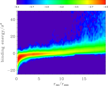
Figure 5.— Logarithm of the number density distribution of the particles in the plane of binding energy versus clustrocentric distance. The top bar shows the color scale, with the number density distribution normalized to the total number of particles in the diagram. Binding energies and clustrocentric distances are normalized to the three-dimensional velocity dispersion $\sigma$ and $r_{200}$ of each individual cluster, respectively. The number density distribution includes all the particles from the entire sample of 2420 mock catalogs.

A galaxy is a cluster member if its binding energy is negative, namely if its velocity $v$ is lower than the velocity $v_{\rm esc}(r)$ required to escape the cluster when the galaxy is at distance $r$ from the cluster center: $v^{2}<v_{\rm esc}^{2}(r)$. Figure 5 shows the number density distribution of the dark matter particles in our mock cluster catalogs in the plane of binding energy versus the three-dimensional (3D) clustrocentric distance. The plot includes the entire sample of 2420 cluster catalogs.

Figure 5 shows that a substantial fraction of bound particles have clustrocentric distance much larger than $r_{200}$ (Wojtak et al. 2007). Therefore, in principle, we might use a different and simpler criterion to define a cluster member: a galaxy whose clustrocentric distance is smaller than, for example, $3r_{200}$. This criterion is actually more restrictive than the criterion based on the binding energy, as Figure 5 suggests. Nevertheless, we include this criterion in the following analysis, for the sake of comparison. Hereafter, we call 3D members these two sets of members defined on the basis of the 3D information.

We expect that the caustic technique identifies the 3D members as the galaxies within the caustics in the redshift diagram. In the following we will also consider a criterion based on the binary tree. As described in Section 2, the caustic technique arranges the galaxies in a binary tree according to their pairwise projected binding energy; by cutting the tree at the $\sigma$ plateau we define a set of candidate members. In the following analysis, we show that the choice of this name is appropriate, because the interloper contamination of this set of candidate members is larger than the contamination of the set of members determined by the caustic location.

In conclusion, we consider two definitions of 3D members: (a) galaxies with negative binding energy; (b) galaxies within $3r_{200}$; and two possible criteria for their identification: (1) galaxies within the caustics in the redshift diagram; (2) galaxies on the main branch of the binary tree cut at the $\sigma$ plateau. Hereafter, we refer to the members identified with methods (1) or (2) as 2D members.

In Sections 4.2 and 4.3 we focus on the performance of the first and second criteria, respectively. We compute two relevant quantities: the completeness $f_{c}$, which is the fraction of 3D members that are also identified as 2D members, and the contamination $f_{i}$, which is the ratio between the number of particles taken as 2D members that are actually interlopers and the total number of 2D members.

4.2. 2D Members: Caustic Location

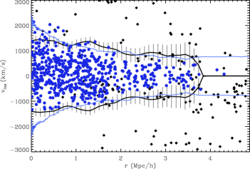
Figure 6.— Redshift diagram of $1000$ particles of a synthetic cluster. The black lines with 1-$\sigma$ error bars and the cyan lines are the estimated and true caustics respectively. The symbols are the particles in the catalog; the blue dots are the bound particles. There are 636 particles between the upper and lower caustics.

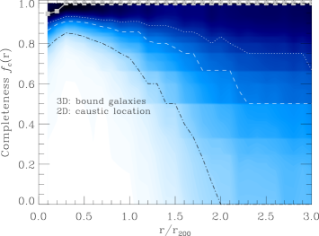
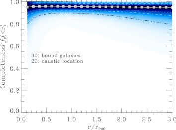
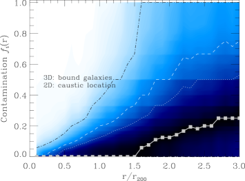
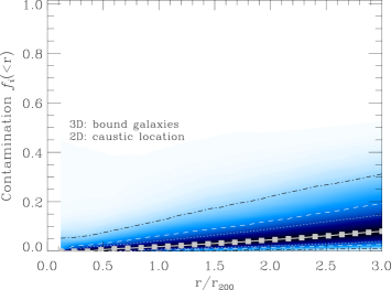
Figure 7.— Upper panels: differential (left panel) and cumulative (right panel) median profiles (solid squares) of the completeness $f_{c}$, where the 3D members are the bound galaxies and the 2D members are the galaxies within the caustics. Lower panels: differential (left panel) and cumulative (right panel) profiles of the contamination $f_{i}$. The darkness of the shaded areas is proportional to the profile number density on the vertical axis. The dotted, dashed, and dot-dashed lines limit the areas including the 50%, 68%, and 90% of the profiles, respectively.

Figure 6 shows the redshift diagram of a cluster from our sample, with the bound galaxies defined as the 3D members, shown as blue dots. As expected, most of the 3D members are within the caustics.

To illustrate how the method performs on average in this case, we compute the completeness and contamination profiles of each cluster. At each radius, we consider the median of the set of profiles and their dispersion. The upper left panel of Figure 7 shows the median differential profile of the completeness $f_{c}$ and the regions containing 50%, 68% and 90% of the profiles.

Only at small radii the caustic algorithm removes a few per cent of the 3D members, because the caustic amplitude is slightly underestimated, as can be seen in the example of Figure 6. The caustic criterion thus provides a completeness close to 0.95 at radii smaller than $0.2r_{200}$, and increases to 1.0 at larger radii.

The median differential contamination (Figure 7, bottom left panel) is larger than 0.1 at radii larger than $2r_{200}$, but the cumulative contamination (Figure 7, bottom right panel) remains below 0.09 at $3r_{200}$. Table 1 gives the corresponding 68% levels for the cumulative profiles of $f_{c}$ and $f_{i}$.

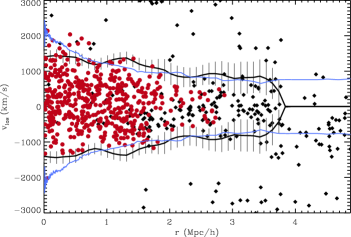
Figure 8.— Same as Figure 6, with red dots the 3D members defined as the particles within the sphere of radius $3r_{200}$.

Figure 8 reproduces the same redshift diagram of Figure 6 with the red dots the particles within $3r_{200}$ from the cluster center defined as the 3D members. In this case, most 3D members are within the caustics, but, at large radii, many particles within the caustics are not 3D members. In fact, in a sample of particles extracted from a spherical halo whose number density profile decreases with radius, the number of particles within a given 3D radius $r$ observed in projection can fall to zero beyond a projected radius $r_{e}\leq r$; obviously, $r_{e}$ decreases with the size of the particle sample. For a Navarro, Frenk, & White (1997) number density profile and for a sample of $185$ particles within $3r_{200}$ (the average number of particles per cluster sample), we find that the number of particles with a 3D distance smaller than $3r_{200}$ is zero at projected distances larger than $r_{e}\sim 2.6r_{200}$. The differential contamination $f_{i}$ for the entire sample remains smaller than 0.1 within $r_{200}$, on average, but increases dramatically at larger radii and reaches $f_{i}=1$ at $r\sim 2.6r_{200}$. It follows that the corresponding cumulative profile of the fraction of galaxies identified as members when they are actually interlopers reaches 0.27 at $3r_{200}$ (Table 1).

On the other hand, the profiles of the completeness we obtain with this definition of 3D members are very similar to Figure 7: the method yields a large ($\sim 0.95$) and stable completeness to radii as large as $3r_{200}$ (Table 1).

4.3. 2D Members: Main Group of the Binary Tree

We now evaluate the completeness $f_{c}$ and the contamination $f_{i}$ of the set of members identified with the binary tree.

With the bound galaxies as the 3D members, the completeness $f_{c}=1.00$ is constant over the entire range of $r$ (Table 1). The median differential contamination $f_{i}$ reaches a maximum value of $\sim 0.4$ at $r>2.5r_{200}$. The cumulative profile thus reaches the value 0.13 (Table 1) at $r=3r_{200}$. The differential profile of $f_{i}$ shows that, if the bound galaxies are taken as 3D members, using the binary tree procedure introduces interlopers at $r>0.8r_{200}$; this result is somewhat worse than the caustic location performance shown in the previous section, because the caustic location, on average, provides samples without contamination up to $r=1.5r_{200}$ (Figure 7). Overall, however, when we adopt the bound particles as 3D member, both the caustic location and the binary tree give high levels of completeness ($f_{c}\sim 0.95-1.0$) and low levels of contamination ($f_{i}\sim 0.08-0.13$) within $3r_{200}$.

In the case of the galaxies within $3r_{200}$ as 3D members (definition (b) in Section 4.1), the completeness $f_{c}$ has a constant median value $f_{c}=1.0$ (Table 1). Clearly, applying the binary tree procedure to determine the members of a cluster guarantees an extremely high completeness of the sample. On the other hand, the median differential contamination $f_{i}$ is smaller than 0.1 at $r<r_{200}$, and increases at larger radii up to $1$. This high contamination at large radii translates into a cumulative $f_{i}$ of 0.31 at $3r_{200}$ (Table 1). The reason for this large contamination at large radii derives from the decreasing of the number density profile, as discussed in Section 4.2.

		bound galaxies						galaxies within $3r_{200}$
Caustic
location		$f_{c}-\sigma$	$f_{c}$	$f_{c}+\sigma$	$f_{i}-\sigma$	$f_{i}$	$f_{i}+\sigma$	$f_{c}-\sigma$	$f_{c}$	$f_{c}+\sigma$	$f_{i}-\sigma$	$f_{i}$	$f_{i}+\sigma$
	$r_{200}$	0.921	0.956	0.984	0.005	0.020	0.066	0.917	0.953	0.983	0.014	0.042	0.118
	$2r_{200}$	0.908	0.951	0.981	0.015	0.047	0.126	0.903	0.947	0.980	0.053	0.125	0.256
	$3r_{200}$	0.875	0.947	0.980	0.027	0.080	0.193	0.898	0.946	0.980	0.143	0.273	0.418

Binary
tree		$f_{c}-\sigma$	$f_{c}$	$f_{c}+\sigma$	$f_{i}-\sigma$	$f_{i}$	$f_{i}+\sigma$	$f_{c}-\sigma$	$f_{c}$	$f_{c}+\sigma$	$f_{i}-\sigma$	$f_{i}$	$f_{i}+\sigma$
	$r_{200}$	0.990	1.000	1.000	0.010	0.031	0.083	0.990	1.000	1.000	0.020	0.050	0.129
	$2r_{200}$	0.981	1.000	1.000	0.034	0.078	0.156	0.984	1.000	1.000	0.073	0.149	0.274
	$3r_{200}$	0.953	0.997	1.000	0.067	0.133	0.233	0.980	1.000	1.000	0.190	0.306	0.443

Table 1Cumulative completeness $f_{c}$ and contamination $f_{i}$ at $r_{200}$, $2r_{200}$, and $3r_{200}$, and their 1-$\sigma$ dispersion, where the 3D members are the bound particles (left) or the particles within $3r_{200}$ (right) and the 2D members are the particles within the caustics (top) or in the main group of the binary tree (bottom).

4.4. Identification of Members in Stacked Clusters

As expected, the results listed in Table 1 indicate that the caustic location is more effective than the binary tree algorithm in identifying 3D members and that the binding energy criterion is more appropriate than the geometrical criterion to define members based on 3D data. Table 1 also shows the spreads of the completeness and contamination. These spreads originate from the random and systematic errors of the caustic technique, which are mostly due to the assumption of spherical symmetry (Serra et al. 2011). In addition, we expect that the performance of the technique depends on the number of galaxies in the catalog.

To quantify these effects, we stack our 3000 mock catalogs and randomly choose particles in the catalog until we obtain a given number $N$ of particles within $3r_{200}$ from the cluster center in real space. The stacking was done by scaling the coordinates with $r_{200}$ and the 3D velocity dispersion of each cluster. Here we show the results for two extreme cases with $N=50$ and $N=200$. We compile 100 different catalogs for each value of $N$ and we apply the procedure to determine the main group of the binary tree and to locate the caustics on the corresponding redshift diagrams. The completeness and contamination profiles are shown in the upper panels of Figure 9 for $N=50$ and in the lower panels for $N=200$. We only show the case where the bound galaxies are the 3D members, and the caustic location is used to select the 2D members. The profiles show that the effect of increasing $N$ from $50$ to $200$ is not significant on the median completeness and contamination profiles, but the associated spreads drop by at least a factor of four for the completeness and a factor of two for the contamination (Table 2).

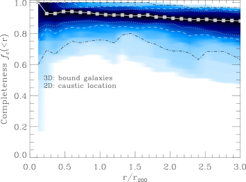
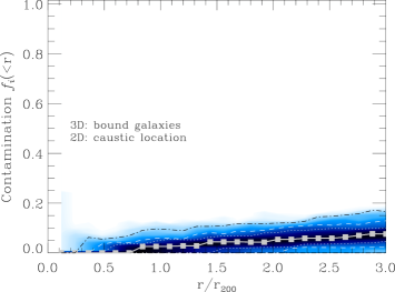
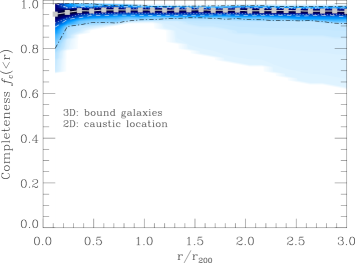
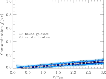
Figure 9.— Cumulative completeness $f_{c}$ (left panels) and contamination $f_{i}$ (right panels), where the 3D members are the bound galaxies and the 2D members are the galaxies within the caustics, for the samples built from the stacked cluster with $N=50$ (upper panels) and $N=200$ (lower panels) particles within $3r_{200}$. The shaded areas and lines are the same as in Figure 7.

		bound galaxies
		$N=50$						$N=200$
Caustic
location		$f_{c}-\sigma$	$f_{c}$	$f_{c}+\sigma$	$f_{i}-\sigma$	$f_{i}$	$f_{i}+\sigma$	$f_{c}-\sigma$	$f_{c}$	$f_{c}+\sigma$	$f_{i}-\sigma$	$f_{i}$	$f_{i}+\sigma$
	$r_{200}$	0.854	0.921	0.971	0.000	0.026	0.059	0.946	0.970	0.982	0.021	0.034	0.052
	$2r_{200}$	0.812	0.898	0.959	0.000	0.055	0.100	0.945	0.967	0.981	0.051	0.071	0.088
	$3r_{200}$	0.758	0.881	0.947	0.022	0.076	0.129	0.939	0.965	0.980	0.080	0.106	0.128

Table 2Cumulative completeness $f_{c}$ and contamination $f_{i}$ at $r_{200}$, $2r_{200}$, and $3r_{200}$ with their corresponding 1-$\sigma$ dispersion, with the bound particles as the 3D members and the particles within the caustics as the 2D members for the stacked cluster with $N=50$ (left) and $N=200$ (right) particles within $3r_{200}$.

5. Mass Estimation

In this section, we analyze the effect of our interloper removal methods on the estimation of the mass, because interlopers have a non-negligible impact on the mass estimation, especially at large radii, where interlopers can cause an overestimate of the mass as large as a factor of three (Perea et al. 1990).

We consider the three standard methods described in Heisler et al. (1985): the virial, the average and the median mass estimators. All estimators assume that the galaxies have equal mass and the system is in a steady state. The virial mass estimator is

$$M_{VT}=\frac{3\pi N}{2G}\frac{\sum_{i}v^{2}_{{\rm los}\,i}}{\sum_{i<j}1/R_{\perp,ij}}$$ (5)

where $N$ is the number of galaxies with measured redshifts, $v_{\rm los}$ is the line-of-sight velocity and $R_{\perp,ij}$ is the projected separation between galaxy $i$ and galaxy $j$. We do not add the surface pressure term in this analysis, because the correction that it introduces is expected to be smaller than $10$% (Rines et al. 2007).

The median mass estimator is supposed to be less sensitive to interlopers, because if interlopers in velocity populate the tails of the distribution of the quantity $(v_{{\rm los}\,i}-v_{{\rm los}\,j})^{2}R_{\perp,ij}$, which is estimated for each of the $N(N-1)/2$ pairs, the median of this quantity is a more robust estimate than the mean. The mass is thus

$$M_{Me}=\frac{f_{Me}}{G}\,{\rm med}\{(v_{{\rm los}\,i}-v_{{\rm los}\,j})^{2}R_{\perp,ij}\}\,,$$ (6)

where the coefficient $f_{Me}=6.5$ is calibrated with $N$-body simulations (Heisler et al. 1985).

If we take the mean, rather than the median, we obtain the average mass estimator

$$M_{\rm AV}=\frac{3f_{\rm AV}}{GN(N-1)}\sum_{i}\sum_{i<j}(v_{{\rm los}\,i}-v_{{\rm los}\,j})^{2}R_{\perp,ij}\,,$$ (7)

where $f_{\rm AV}=2.8$ is again calibrated with $N$-body simulations (Heisler et al. 1985). As mentioned above, one expects that the virial and average mass estimators are more sensitive to interlopers than the median mass estimator.

We apply these three estimators to our samples after removing the interlopers with our two different procedures: (1) the caustic location and (2) the binary tree.

The top panel of Figure 10 shows the results of applying the mass estimators to individual clusters within $r_{200}$, $2r_{200}$ and $3r_{200}$. On average, the mass estimate is unbiased when the member galaxies are identified with the caustic location, whereas it is biased high by at least 20% when the member galaxies are extracted from the main group of the binary tree. This result confirms our expectation that the caustic location removes interlopers more efficiently than the binary tree procedure. As expected, the median mass estimator is the less sensitive method to the presence of interlopers: in fact, it yields the values of $M_{\rm est}/M_{\rm true}$ closest to one when the interlopers are removed with the less efficient binary tree procedure.

For comparison, we also show the mass estimated with the caustic technique applied to the full sample of particles, because, in principle, the technique is not affected by the presence of interlopers. With all the estimators, the spread increases with radius. For the caustic technique, this increase derives from the smaller number of galaxies available for locating the caustics. For the other estimators the system is required to be in virial equilibrium, that does not necessarily hold at radii larger than $r_{200}$; therefore, at these radii, the three standard estimators are more likely to return an incorrect mass.

In addition, part of these spreads derives from the assumption of spherical symmetry. The bottom panels of Figure 10 show the mass estimates of the stacked clusters with $N=50$ and $N=200$. The spreads for the case $N=50$ are slightly smaller than in the case of individual clusters (upper panel of Figure 10), despite the fact that, on average, individual clusters have 185 galaxies within $3r_{200}$, a factor of 3.7 larger than the $N=50$ stacked cluster (bottom left panel of Figure 10). In the stacked clusters, the assumption of spherical symmetry is basically correct, therefore the spread only derives from the sample size. In fact, the spreads further reduce by a factor of roughly $25$% in the case of the $N=200$ stacked cluster (bottom right panel of Figure 10).

We finally note that in the case $N=50$, the mass estimate is biased low by 20%. In this case, in fact, the number of galaxies within $r_{200}$ is only $27$, on average, and the velocity field is too poorly sampled to return a correct mass.

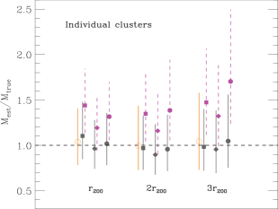
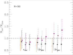
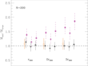
Figure 10.— Ratios $M_{\rm est}/M_{\rm true}$ between the cluster mass estimated with various methods and the true mass derived from the $N$-body simulation. The mass estimators are applied to individual clusters within $r_{200}$, $2r_{200}$ and $3r_{200}$ (top panel) and to the stacked clusters with $N=50$ and $N=200$ (bottom panels). $M_{\rm est}$ is estimated with the virial theorem (squares), the median (diamonds) or the average (solid circles) mass estimators; the interlopers are removed with the caustic location (gray), or the binary tree (violet). The error bars show the 68% range of the distributions. The open circles show the mass estimated with the caustic technique on the full particle sample, because the caustic technique mass is not affected, in principle, by the presence of interlopers.

6. Discussion

Proper estimates of the mass of galaxy clusters and of the properties of their galaxy population depend on the accurate separation between the cluster members and those galaxies that appear projected in the cluster field of view but are not dynamically linked to the cluster.

Numerous methods to identify and remove interlopers in galaxy clusters have been suggested in the literature. The algorithms are based either on the line-of-sight velocity separation of the galaxy from the cluster center alone or on both the velocity and the projected separations. The former class of algorithms is suited for galaxy samples that only survey the central regions of the clusters. These algorithms include the $3\sigma$ clipping method (Yahil & Vidal 1977), which assumes that the velocity distribution is close to Gaussian, the gap method (Zabludoff et al. 1990; Beers et al. 1990), and the adaptive kernel method (Pisani 1993). However, not all interlopers have large velocity separations from the cluster, as Figure 6 illustrates. These interlopers are difficult to identify and can generate a rather counterintuitive systematic error: they can cause a slight underestimate, rather than an overestimate, of the cluster velocity dispersion (Cen 1997; Diaferio et al. 1999; Biviano et al. 2006).

Rather than iterating over the velocity dispersion, like the $3\sigma$ clipping method does, one can iterate over the virial mass: at each step, one removes the galaxy that causes the largest mass variation (Perea et al. 1990). The projected and virial mass estimators (Heisler et al. 1985) are sensitive to the presence of interlopers in different ways; comparing their mass values can also be used to identify interlopers (Wojtak et al. 2007). Iterating over the mass provides more robust results than iterating over the velocity dispersion, because interlopers can affect more the estimate of the size of the cluster, which enters the mass estimate, than the velocity dispersion (Diaferio et al. 1999).

When galaxy catalogs survey large cluster regions, the methods described above can be extended and applied to galaxy subsamples separated into bins of projected distances to the cluster center (Fadda et al. 1996). Thus, the velocity distribution assumed to be Gaussian at each radius can have different widths at different radii (Prada et al. 2003), or the velocity dispersion in the $3\sigma$ clipping method can be derived at different radii by solving the Jeans equation for a steady state system and isotropic galaxy orbits (Łokas et al. 2006).

A step forward an interloper rejection algorithm based on a dynamical approach derives from the following consideration: from an extensive galaxy sample we can actually extract information on the dependence of the escape velocity on the clustrocentric distance (den Hartog & Katgert 1996). Based on this idea, most algorithms first estimate the mass profile by assuming dynamical equilibrium, and then, from these mass profiles, derive the escape velocity as a function of the projected distance to the cluster center. The final solution thus must be obtained by iteratively removing the identified interlopers until the mass profile converges.

Here, we have shown the performance of the caustic technique, used as an interloper rejection algorithm. The technique only uses the number density distribution of galaxies in the redshift diagram to estimate directly the escape velocity profile from the system. Unlike the methods mentioned above, the caustic technique relies neither on the assumption of dynamical equilibrium nor on the estimate of the mass profile. Therefore, the technique does not require any iteration; in addition, the estimate of the cluster mass profile is a further step that is unnecessary for identifying the interlopers and it is a step that we have not taken here.

In the presence of extensive surveys, interloper rejection algorithms based on the estimate of the mass or on the escape velocity usually perform better than algorithms solely based on the velocity distribution (e.g., Wojtak & Lokas 2007; Wojtak et al. 2007; White et al. 2010). Wojtak et al. (2007) perform an extensive comparison of a number of different algorithms. They conclude that the method by den Hartog & Katgert (1996) is the most effective at removing interlopers, producing samples with average contaminations $f_{i}$ in the range $0.02-0.04$ within one projected virial radius.

These values are in perfect agreement with our median $f_{i}=0.02$ (Table 1). However, there are two noticeable differences between our analysis and theirs: the dynamical state of the clusters and the sample extension. The caustic technique is independent of the dynamical state of the cluster, and, in fact, we only adopt the cluster mass as the criterion to build our sample of $100$ simulated clusters. On the contrary, in their sample of $10$ simulated clusters, Wojtak et al. (2007) pay particular attention to only include relaxed systems that have no sign of ongoing mergers, because the den Hartog & Katgert (1996) method requires dynamical equilibrium to be effective. Merging clusters require more sophisticated approaches (see, e.g., Wegner 2011 and references therein), like the caustic technique.

In addition, the dynamical equilibrium assumption clearly limits the analysis to projected radii smaller than the virial radius, where the equilibrium is expected to hold, whereas the caustic technique enables the identification of interlopers to much larger radii. We find that, with the caustic technique, the median contamination increases to $f_{i}=0.047$ and $0.080$ at $2r_{200}$ and $3r_{200}$, respectively, with a median completeness $f_{c}$ that remains larger than $\sim 0.95$. No other methods that remove interlopers in these regions are currently available.

When we use the caustic technique to identify interlopers, the virial mass estimator returns a mass overestimated by 10% within $r_{200}$, similarly to the results of Biviano et al. (2006), who removed interlopers with a combination of the gap procedure (Girardi et al. 1993) and the method of den Hartog and Katgert (Katgert et al. 2004; den Hartog & Katgert 1996) from mock clusters with more than 60 members. This bias is not present when we use the median and average mass estimators. At radii larger than $r_{200}$, where only the caustic technique can be used to remove interlopers, all mass estimates are unbiased.

7. Conclusion

The caustic technique identifies the escape velocity profiles of galaxy clusters to radii as large as $3r_{200}$; we can thus estimate the cluster mass in regions where the cluster is not necessarily in dynamical equilibrium. The performance of the caustic method as a mass estimator has been tested on both $N$-body simulations (Diaferio & Geller 1997; Diaferio et al. 1999; Serra et al. 2011) and real clusters (Diaferio et al. 2005; Geller et al. 2013), regardless of their dynamical state: when we compare the caustic mass with the gravitational lensing mass in a combined sample of 22 clusters, the two estimates generally agree (Diaferio et al. 2005; Geller et al. 2013).

Here, we have investigated an additional use of the caustic technique: the interloper rejection method. In this case, the technique relies only on the location of the caustics on the redshift diagram and makes no use of the mass profile of the cluster. We have tested the ability of the method to identify the cluster galaxy members by using $100$ galaxy clusters with mass $M_{200}\geq 10^{14}h^{-1}M_{\odot}$ extracted from a cosmological $N$-body simulation of a $\Lambda$CDM universe. Unlike the case of the mass estimate, where we compare the caustic technique with gravitational lensing, we cannot test the interloper rejection method on real clusters. However, the caustic technique is based on the hypothesis that clusters form by hierarchical clustering; wide observational evidence, based on X-ray and optical data, including gravitational lensing studies (e.g. Diaferio et al. 2008; Borgani & Kravtsov 2011), suggest that this hypothesis is well founded. Therefore we expect that $N$-body simulated clusters are a reasonable representation of real clusters and that the results of our analysis can be safely applied to real clusters.

Our mock catalogs contain 1000 galaxies in the field of view of $12h^{-1}$ Mpc on a side at the cluster location. The true 3D members, defined as the gravitationally bound galaxies, are compared to the galaxies identified as members with the caustic technique. We find a completeness of $f_{c}=0.95\pm 0.03$ within $3r_{200}$, whereas the contamination increases from $f_{i}=0.020^{+0.046}_{-0.015}$ at $r_{200}$ to $f_{i}=0.08^{+0.11}_{-0.05}$ at $3r_{200}$. The lack of spherical symmetry in clusters of galaxies causes most of the spread of the completeness and the contamination profiles. In fact, when applying the technique to samples built from a spherically symmetric stacked cluster the spreads decrease by at least a factor of two. No other technique for the identification of the members of a galaxy cluster provides such large completeness and small contamination at these large radii.

The mass estimated with the virial theorem within $3r_{200}$, after removing interlopers in the case of individual clusters, is unbiased and is within 30% of the actual mass. The use of the spherically symmetric stacked cluster decreases the spread to less than 10%.

For the sake of clarity, we remind the systematic error that our interloper rejection method can introduce: the membership identification is based on identifying the caustic amplitude with the escape velocity tout-court, whereas the caustic amplitude, which we measure independently of the knowledge of $g(\beta)$, of the mass profile and of the gravitational potential profile, actually is the escape velocity corrected by the factor $g^{-1/2}(\beta)$ (Equation 2). The fact that we neglect this correction factor when we identify the caustic amplitude with the escape velocity can propagate in an incorrect separation of the cluster members from the interlopers. Our excellent results show that, despite this simplification, the caustic method can satisfactorily separate the members from the interlopers.

The increasing amount of data in clusters of galaxies (Geller et al. 2011) requires adequate tool for extracting the information they contain and properly comparing them with the output of the galaxy formation modeling that is increasingly sophisticated (Saro et al. 2012).

The caustic technique can provide accurate estimates of the dark matter distribution in the outer regions of galaxy clusters and information on the dynamical connection between galaxies and clusters. The first piece of information is relevant for our understanding of the formation of cosmic structure and can even constrain the properties of dark matter (Serra & Domínguez Romero 2011) and the theory of gravity (Lam et al. 2012).

Determining the membership of galaxies in the outskirts of clusters is unique to the caustic method. Applying the algorithm to a large sample of clusters can provide the first accurate measure of how the gradients of properties of the cluster galaxy population, such as color and star formation rate, merge into the field. In addition, it might provide the first determination of galaxy membership in the filaments surrounding clusters that represent the preferred path of mass accretion (Pimbblet et al. 2004; Colberg et al. 2005; Aragón-Calvo et al. 2010; González & Padilla 2010); this piece of information can thus enlighten the connection between the formation of galaxies and the large-scale structure. In future work, we will investigate the reliability of the caustic method in performing these measurements and assess the impact that these measures can have on the models of the formation of the cosmic structure.

References

- Aragón-Calvo et al. (2010) Aragón-Calvo, M. A., van de Weygaert, R., & Jones, B. J. T. 2010, MNRAS, 408, 2163
- Beers et al. (1990) Beers, T. C., Flynn, K., & Gebhardt, K. 1990, AJ, 100, 32
- Benatov et al. (2006) Benatov, L., Rines, K., Natarajan, P., Kravtsov, A., & Nagai, D. 2006, MNRAS, 370, 427
- Biviano et al. (2006) Biviano, A., Murante, G., Borgani, S., Diaferio, A., Dolag, K., & Girardi, M. 2006, A&A, 456, 23
- Borgani (2008) Borgani, S. 2008, in A Pan-Chromatic View of Clusters of Galaxies and the Large-Scale Structure, ed. M. Plionis, O. López-Cruz, & D. Hughes, Vol. 740, 287
- Borgani & Kravtsov (2011) Borgani, S., & Kravtsov, A. 2011, ASL, 4, 204
- Borgani et al. (2004) Borgani, S., et al. 2004, MNRAS, 348, 1078
- Brown et al. (2010) Brown, W. R., Geller, M. J., Kenyon, S. J., & Diaferio, A. 2010, AJ, 139, 59
- Cen (1997) Cen, R. 1997, ApJ, 485, 39
- Colberg et al. (2005) Colberg, J. M., Krughoff, K. S., & Connolly, A. J. 2005, MNRAS, 359, 272
- den Hartog & Katgert (1996) den Hartog, R., & Katgert, P. 1996, MNRAS, 279, 349
- Diaferio (1999) Diaferio, A. 1999, MNRAS, 309, 610
- Diaferio (2009) —. 2009, ArXiv e-prints: 0901.0868
- Diaferio & Geller (1997) Diaferio, A., & Geller, M. J. 1997, ApJ, 481, 633
- Diaferio et al. (2005) Diaferio, A., Geller, M. J., & Rines, K. J. 2005, ApJ Lett., 628, L97
- Diaferio et al. (2001a) Diaferio, A., Kauffmann, G., Balogh, M. L., White, S. D. M., Schade, D., & Ellingson, E. 2001a, MNRAS, 323, 999
- Diaferio et al. (2001b) —. 2001b, MNRAS, 323, 999
- Diaferio et al. (1999) Diaferio, A., Kauffmann, G., Colberg, J. M., & White, S. D. M. 1999, MNRAS, 307, 537
- Diaferio et al. (2008) Diaferio, A., Schindler, S., & Dolag, K. 2008, SSRv, 134, 7
- Diemand et al. (2004) Diemand, J., Moore, B., & Stadel, J. 2004, MNRAS, 352, 535
- Domínguez et al. (2001) Domínguez, M., Muriel, H., & Lambas, D. G. 2001, AJ, 121, 1266
- Fadda et al. (1996) Fadda, D., Girardi, M., Giuricin, G., Mardirossian, F., & Mezzetti, M. 1996, ApJ, 473, 670
- Geller et al. (2011) Geller, M. J., Diaferio, A., & Kurtz, M. J. 2011, AJ, 142, 133
- Geller et al. (2013) Geller, M. J., Diaferio, A., Rines, K. J., & Serra, A. L. 2013, ApJ, 764, 58
- Gill et al. (2005) Gill, S. P. D., Knebe, A., & Gibson, B. K. 2005, MNRAS, 356, 1327
- Gill et al. (2004) Gill, S. P. D., Knebe, A., Gibson, B. K., & Dopita, M. A. 2004, MNRAS, 351, 410
- Girardi et al. (1993) Girardi, M., Biviano, A., Giuricin, G., Mardirossian, F., & Mezzetti, M. 1993, ApJ, 404, 38
- González & Padilla (2010) González, R. E., & Padilla, N. D. 2010, MNRAS, 407, 1449
- Heisler et al. (1985) Heisler, J., Tremaine, S., & Bahcall, J. N. 1985, ApJ, 298, 8
- Hernández-Fernández et al. (2012) Hernández-Fernández, J. D., Vílchez, J. M., & Iglesias-Páramo, J. 2012, ApJ, 751, 54
- Huertas-Company et al. (2009) Huertas-Company, M., Foex, G., Soucail, G., & Pelló, R. 2009, A&A, 505, 83
- Hwang et al. (2012) Hwang, H. S., Geller, M. J., Diaferio, A., & Rines, K. J. 2012, ApJ, 752, 64
- Kaiser (1987) Kaiser, N. 1987, MNRAS, 227, 1
- Katgert et al. (2004) Katgert, P., Biviano, A., & Mazure, A. 2004, ApJ, 600, 657
- Lam et al. (2012) Lam, T. Y., Nishimichi, T., Schmidt, F., & Takada, M. 2012, PhRvL, 109, 051301
- Lemze et al. (2009) Lemze, D., Broadhurst, T., Rephaeli, Y., Barkana, R., & Umetsu, K. 2009, ApJ, 701, 1336
- Łokas et al. (2006) Łokas, E. L., Wojtak, R., Gottlöber, S., Mamon, G. A., & Prada, F. 2006, MNRAS, 367, 1463
- Mahajan & Raychaudhury (2009) Mahajan, S., & Raychaudhury, S. 2009, MNRAS, 400, 687
- Martínez et al. (2008) Martínez, H. J., Coenda, V., & Muriel, H. 2008, MNRAS, 391, 585
- Navarro et al. (1997) Navarro, J. F., Frenk, C. S., & White, S. D. M. 1997, ApJ, 490, 493
- Perea et al. (1990) Perea, J., del Olmo, A., & Moles, M. 1990, A&A, 237, 319
- Pimbblet et al. (2004) Pimbblet, K. A., Drinkwater, M. J., & Hawkrigg, M. C. 2004, MNRAS, 354, L61
- Pisani (1993) Pisani, A. 1993, MNRAS, 265, 706
- Prada et al. (2003) Prada, F., et al. 2003, ApJ, 598, 260
- Regös & Geller (1989) Regös, E., & Geller, M. J. 1989, AJ, 98, 755
- Rines & Diaferio (2006) Rines, K., & Diaferio, A. 2006, AJ, 132, 1275
- Rines et al. (2007) Rines, K., Diaferio, A., & Natarajan, P. 2007, ApJL, 657, 183
- Rines et al. (2008) —. 2008, ApJ, 679, L1
- Rines et al. (2013) Rines, K., Geller, M. J., Diaferio, A., & Kurtz, M. J. 2013, ApJ, 767, 15
- Rines et al. (2004) Rines, K., Geller, M. J., Diaferio, A., Kurtz, M. J., & Jarrett, T. H. 2004, AJ, 128, 1078
- Rines et al. (2000) Rines, K., Geller, M. J., Diaferio, A., Mohr, J. J., & Wegner, G. A. 2000, AJ, 120, 2338
- Rines et al. (2003) Rines, K., Geller, M. J., Kurtz, M. J., & Diaferio, A. 2003, AJ, 126, 2152
- Rines et al. (2005) —. 2005, AJ, 130, 1482
- Saro et al. (2012) Saro, A., Bazin, G., Mohr, J., & Dolag, K. 2012, ArXiv:astro-ph/1203.5708
- Serra et al. (2010) Serra, A. L., Angus, G. W., & Diaferio, A. 2010, A&A, 524, A16
- Serra et al. (2011) Serra, A. L., Diaferio, A., Murante, G., & Borgani, S. 2011, MNRAS, 412, 800
- Serra & Domínguez Romero (2011) Serra, A. L., & Domínguez Romero, M. J. L. 2011, MNRAS, 415, L74
- Skibba et al. (2009) Skibba, R. A., et al. 2009, MNRAS, 399, 966
- Springel (2005) Springel, V. 2005, MNRAS, 364, 1105
- van Haarlem & van de Weygaert (1993) van Haarlem, M., & van de Weygaert, R. 1993, ApJ, 418, 544
- Voit (2005) Voit, G. M. 2005, RvMP, 77, 207
- Wegner (2011) Wegner, G. A. 2011, MNRAS, 413, 1333
- White et al. (2010) White, M., Cohn, J. D., & Smit, R. 2010, MNRAS, 408, 1818
- Wojtak & Lokas (2007) Wojtak, R., & Lokas, E. L. 2007, ArXiv:astro-ph/0712.2698
- Wojtak et al. (2007) Wojtak, R., Łokas, E. L., Mamon, G. A., Gottlöber, S., Prada, F., & Moles, M. 2007, A&A, 466, 437
- Yahil & Vidal (1977) Yahil, A., & Vidal, N. V. 1977, ApJ, 214, 347
- Yegorova et al. (2011) Yegorova, I. A., Pizzella, A., & Salucci, P. 2011, A&A, 532, A105
- Zabludoff et al. (1990) Zabludoff, A. I., Huchra, J. P., & Geller, M. J. 1990, ApJS, 74, 1
- Zhang et al. (2011) Zhang, Y.-Y., Andernach, H., Caretta, C. A., Reiprich, T. H., Böhringer, H., Puchwein, E., Sijacki, D., & Girardi, M. 2011, A&A, 526, A105
- Zhang et al. (2012) Zhang, Y.-Y., Verdugo, M., Klein, M., & Schneider, P. 2012, A&A, 542, A106