On-Orbit Sensitivity Evolution of the EUV Imaging Spectrometer on Hinode

Abstract

Since its launch on 22 September 2006, the EUV Imaging Spectrometer onboard the Hinode satellite has exhibited a gradual decay in sensitivity. Using spectroheliograms taken in the Fe viii 185.21 Å and Si vii 275.35 Å emission lines in quiet regions near Sun center we characterize that decay. For the period from December 2006 to March 2012, the decline in the sensitivity can be characterized as an exponential decay with an average time constant of $7358\pm 1030$ days ($20.2\pm 2.8$ years). Emission lines formed at temperatures $\gsim\!10^{6.1}$ K in the quiet-Sun data exhibit solar-cycle effects.

1 Introduction

s:introduction

The EUV Imaging Spectrometer (EIS) on the Hinode satellite [Kosugi et al. (2007)] observes emission lines of highly ionized elements in two wavelength bands with the aim of using line intensity, profile, and Doppler shift data to characterize plasma properties in the solar atmosphere at temperatures ranging from $\approx\!40,000$ K to $\approx\!20$ MK [Culhane et al. (2007)]. All of the individual components of EIS were characterized before final instrument assembly, and the instrument underwent end-to-end testing and calibration [Korendyke et al. (2006), Lang et al. (2006)]. These data were used to compute effective area curves for each EIS wavelength band.

After end-to-end testing, EIS was shipped to Japan in August 2004, stored in a controlled environment at the Japanese Aerospace Exploration Agency, integrated onto the Hinode satellite, and launched on 22 September 2006. During this time interval, it was not possible to monitor the status of the instrument calibration. On orbit, EIS was allowed to outgas for 30 days, and the first spectra were acquired on 28 October 2006.

All previous solar EUV spectrometers have exhibited sensitivity degradation over time. Thus, early in the mission, the EIS team initiated a program of regular quiet-Sun observations of selected EUV lines to monitor the instrument sensitivity. This article reports on an analysis of those data.

2 Observations and Data Processing

s:observations

EIS observes the solar EUV spectrum in two 40-Å wavelength bands centered at 195 and 270 Å. Each spectrum is stigmatic along the slit, which is oriented in the N – S direction. The instrument produces line profiles by imaging the Sun onto two slits ($1\hbox{${}^{\prime\prime}$}$ and $2\hbox{${}^{\prime\prime}$}$), and monochromatic images by imaging the Sun onto two slots ($40\hbox{${}^{\prime\prime}$}$ and $266\hbox{${}^{\prime\prime}$}$). Moving a fine mirror mechanism allows EIS to construct spectroheliograms in selected emission lines by rastering regions of interest. Culhane2007ex provide an extensive discussion of EIS and its operation.

From 6 April 2007 through 28 January 2008, EIS regularly obtained spectroheliograms covering $128\hbox{${}^{\prime\prime}$}\times 184\hbox{${}^{\prime\prime}$}$ with a step size of $1\hbox{${}^{\prime\prime}$}$ in quiet-Sun regions generally near Sun-center (EIS study SYNOP002). Each 90-second exposure covered the entire wavelength range of both CCDs. From each exposure, 14 wavelength windows containing relatively strong lines and covering the wavelength ranges of both detectors were extracted for further analysis.

Early in 2008, the Hinode X-band transmitter failed and data transmission from the satellite had to rely on the slower S-band transmitter. In response to the reduced data rates the EIS team shifted to a new monitoring study (SYNOP006), which had the same raster size and exposure time but only retrieved data from the 14 wavelength windows that were being analyzed using data from the earlier study. Aside from the change to transmitting just the 14 wavelength windows, the new study was identical to the earlier one.

Since it is possible that significant sensitivity loss occurred early in the mission, the studies outlined above were supplemented by searching the EIS data for similar spectroheliograms taken near Sun center from early in the mission until April 2007, when the first synoptic study was initiated. These data usually did not contain all of the lines captured in the synoptic studies, but they provide significant useful information on the instrument sensitivity changes early in the mission.

All of the data sets used in this study were processed using the standard EIS data reduction software. This software removes detector bias and dark current, hot pixels, dusty pixels, and cosmic rays, and then applies the prelaunch absolute calibration. This results in sets of intensities in erg cm^-2 s^-1 sr^-1 Å^-1. All of the emission lines, with the exception of He ii 256.317 Å, are isolated features. Thus, in principle, it is possible to compute the total intensity in each line by simply summing the pixel values with the background subtracted. This approach, however, does not provide any simple measure of which profiles are unacceptable because, for example, of improperly removed artifacts or cosmic ray hits. Instead, for each selected wavelength window, the emission line data were fitted with Gaussian line profiles plus a constant background. This has the advantage of providing an indication of the goodness of the fit, which can be used to exclude bad data. The resulting total line-intensity values are the basic data used in this analysis. Table tbl:lines lists the emission lines used in this study along with their temperature of formation. The additional columns in the table will be discussed later in this article.

Table 1.: Emission lines used in this study and estimated intensities on 6 November 2007. The errors listed for the EIS intensities were computed by taking the standard deviation of the residuals between the model for the EIS sensitivity decline and the observed data.tbl:lines

Ion	$\lambda$	$\log T_{\mathrm{e}}$	$I$	$I_{\mathrm{cal}}$
	[Å]	[K]	[erg cm-2 s-1 sr-1]
He ii	256.317	4.85	$169\pm 19$	…
Fe viii	185.213	5.65	0$27\pm 5.5$	0$36\pm 3.6$
Si vii	275.352	5.80	0$14\pm 2.9$	…
Fe x	184.536	6.00	0$76\pm 17$	$122\pm 12$
Fe xi	180.401	6.10	$199\pm 52$	$345\pm 34$
Fe xii	193.509	6.15	0$64\pm 35$	0$95\pm 9.5$
Fe xii	195.119	6.15	0$89\pm 47$	…
Si x	258.375	6.15	0$31\pm 9.6$	…
Fe xiii	202.044	6.20	0$47\pm 47$	…

Figure fig:rasters shows an example of some of the intensity spectroheliograms obtained from one of the data sets used in this work. The spectroheliograms exhibit the typical features of the quiet Sun seen in lines formed in the transition region and corona. In the transition region, lines such as those of He ii and Fe viii exhibit the well-known cell-network pattern with some areas of network being significantly brighter than the overall average. Coronal lines such as those of Fe x and Fe xii show a smoother emission pattern, but some of the brighter network emission locations are also bright at the higher temperatures.

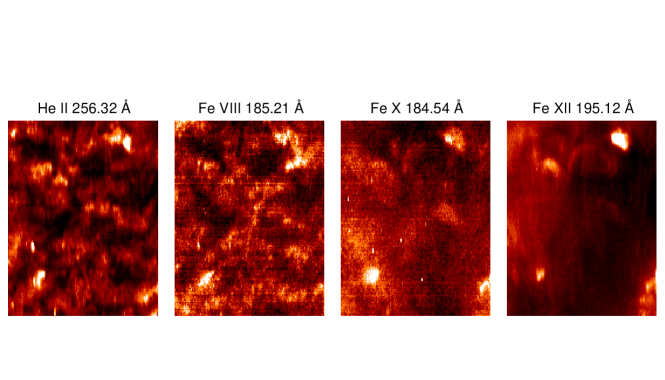
Figure 1.: Spectroheliograms constructed from data taken starting at 14:33:20 on 7 January 2008. The images have dimensions of 128^′′ in the $x$-direction and 166^′′ in the $y$-direction, and are centered at an ($x$,$y$) position on the Sun of ($-290\hbox{${}^{\prime\prime}$}$, $577\hbox{${}^{\prime\prime}$}$). The $y$-direction size is smaller than the true $y$-dimension of the data because some of the rows are lost when the offset between the two detectors is used to co-register the data.fig:rasters

Each year from roughly late April until late August (the beginning and ending dates are changing as the orbit changes), Hinode passes through the Earth’s shadow each orbit. Since a full synoptic study takes more than an orbit to complete, some of the exposures will be compromised. These exposures were removed from the data set by visually inspecting plots of the total intensity in each exposure as a function of the solar $x$-position in the Fe xii 195 Å fitted intensity data. Exposures with incomplete data were also removed.

The standard EIS data-reduction software includes an estimate of the error for each pixel in an exposure, and these errors are used by the fitting software to determine the reduced $\chi^{2}$ for the fit. This error estimate consists of the noise due to photon statistics and an estimate of the dark-current uncertainty combined in quadrature. For well-behaved line profiles the average values of the reduced $\chi^{2}$ are generally around 0.5 rather than the expected value of 1.0. This effect was also noted in CDS data by Thompson2000, who suggested a renormalization procedure for the CDS error estimates. The details of making adjustments in the EIS errors are still under study. For this work, all intensities for which the reduced $\chi^{2}$ for the fit is greater than 1.0 have been excluded.

The He ii 256.317 Å emission line (actually a blend of lines at 256.317 Å and 256.318 Å) is particularly challenging to fit. On its long-wavelength side the line is blended with several coronal lines. According to the CHIANTI database [Dere et al. (1997), Landi et al. (2012)], the lines are Si X at 256.378 Å, Fe x at 256.398 Å, Fe xiii at 256.400 Å, and Fe xii at 256.410 Å. In quiet solar regions, the He ii line is significantly stronger than the other lines and they can be represented by a second Gaussian, which is mostly emission from the Si x line. Brighter locations in the spectroheliograms often have somewhat stronger emission from the hotter lines, and the fitting process then can become challenging.

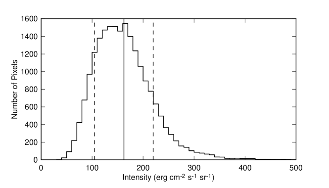
Figure 2.: The distribution of He ii 256.317 Å line intensities for the 7 January 2008 data shown in Figure fig:rasters.fig:sample-avg

For each spectroheliogram in each emission line, the line intensities in the acceptable spatial pixels display a range of intensities. As an example, Figure fig:sample-avg shows a histogram of the distribution of He ii 256.317 Å intensities in the data set shown in Figure fig:rasters. The histogram displays the characteristics typical of emission lines from the upper chromosphere and lower transition region (e.g. Reeves1976; Schrijver1985). The number of pixels at a given intensity rises rapidly to a broad peak and then exhibits an extended higher-intensity tail compared with the rising part of the histogram. This behavior is a characteristic of a log-normal intensity distribution (e.g. Warren2005a). A solid line in the figure marks the mean intensity for the spectroheliogram. Dashed lines show one standard deviation around the mean. For this spectroheliogram, the average intensity is 162 erg cm^-2 s^-1 sr^-1 with a standard deviation of 57.4 erg cm^-2 s^-1 sr^-1. This value for the standard deviation is typical for most of the He ii spectroheliograms and is a reflection of the range of intensities seen in the quiet Sun. The width of the Gaussian characteristic of the log-normal distribution represented by the data in Figure fig:sample-avg is 0.15, comparable to the values tabulated in Warren2005a. Histograms for other emission lines display similar behavior for the cooler lines. For the hottest lines considered in this study, those with a temperature of formation above that of Fe xii, the histograms often have more than one peak, showing the influence of small regions of enhanced emission in the spectroheliogram.

3 Analysis

s:analysis

For each data set and emission line listed in Table tbl:lines average intensities and standard deviations were computed in the manner outlined above. Figure fig:time-hist displays the temporal behavior of the averages for nine of the 14 emission lines captured in the standard monitoring studies. The data in both the figure and in Table tbl:lines are ordered by the temperature of formation of the emission lines rather than by wavelength. To show better the range of intensity variations among the emission lines, all of the data have been plotted using the same range of values on the $y$-axes. Averages for the higher-temperature emission lines, those of Fe xi, Fe xii, Si x, and Fe xiii show an initial decline in average intensity as a function of time, but then show an increasing average intensity as a function of time after some time in 2009. The NOAA Space Weather Prediction Center lists December 2008 as the date of the recent solar minimum. Thus it appears that even in quiet solar regions the hotter emission lines are affected by the solar cycle. This effect has already been noted by Kamio2012. Averages for the lower-temperature emission lines in the figure, those of He ii, Fe viii, Si vii, and Fe x, show declining average intensities as a function of time for the entire time period.

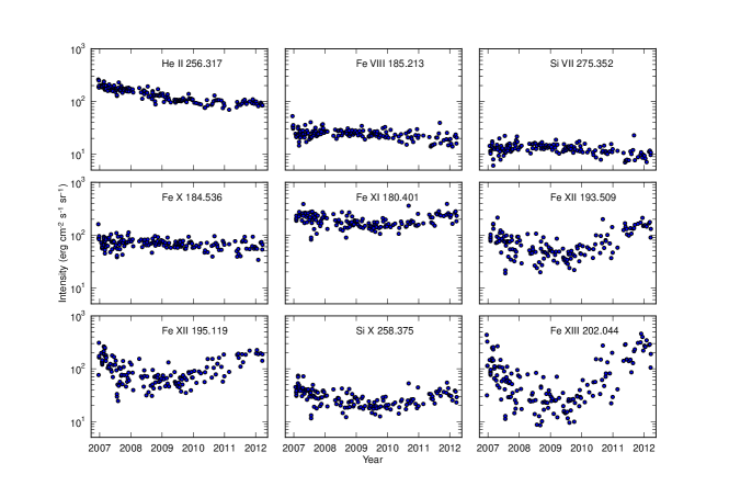
Figure 3.: Average line intensities as a function of time for a selection of the emission lines observed in the EIS monitoring studies.fig:time-hist

The slope of the initial decline in average intensities for the higher temperature lines is generally steeper at the higher temperatures than at the lower temperatures. For the emission lines of Fe viii, Si vii, and Fe x the slopes are similar, with the average intensities declining by about 25 % over the time period of the observations.

The average emission in the He ii 256 Å emission line is somewhat different. As we noted earlier, this line is challenging to fit accurately. The He ii data shown in Figure fig:time-hist are for only the 256.317 Å component of the fit. These data show a somewhat different behavior than the emission from the next three hottest lines of Fe viii, Si vii, and Fe x. The initial decline of the He ii emission is more rapid than those two lines, but then the trend flattens and there is a much smaller decrease in the last two years of data. The similarity of the initial decline to the behavior of the hotter coronal lines suggests that the two-component fits to the He ii data have not been fully successful at separating the 256.317 Å emission line from the hotter emission lines.

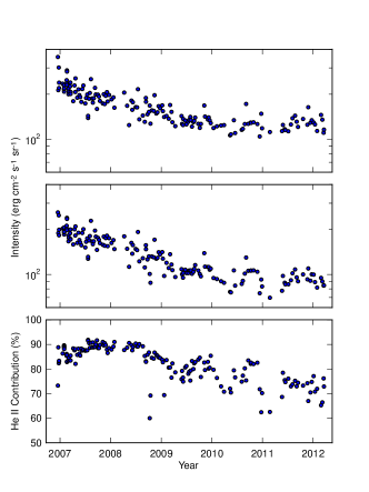
Figure 4.: He ii 256.317 Å line intensities as a function of time. The top panel is the total intensity obtained using a two-component fit to the data, the middle panel shows the He ii 256.317 Å component only, and the bottom panel shows the percentage contribution of that component to the total intensity.fig:he-panel

Figure fig:he-panel shows the He ii 256.317 Å data, the total intensity in the line profile, and the percentage of the emission coming from the 256.317 Å component as a function of time. Both the total intensity and the 256.317 Å component show the rapid decline. As that decline takes place, the contribution of the He ii component decreases. This is consistent with the solar-cycle behavior exhibited by the coronal emission lines of Fe xii, Si i, and Fe xiii. In fact, if the He ii 256.317 Å averaged intensities are assumed to be characteristic of the decline in EIS sensitivity and are used to detrend the other data, then the resulting intensities in the Fe viii, Si vii, and Fe x increase throughout the time period of the observations. Since the solar minimum did not occur until the end of 2008, this behavior is not plausible. We therefore conclude that, despite the fact that the He ii emission line is formed at a lower temperature than any of the other emission lines used in this study and should therefore be less subject to solar-cycle effects, the uncertainties in removing the coronal emission from the line intensities result in a data set that is seriously compromised.

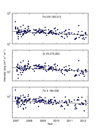
Figure 5.: Average line intensities in the Fe viii, Si vii, and Fe x emission lines. The lines on each plot show the results of an exponential fit to each data set.fig:cool-fit-plots

Since the He ii data are compromised, the other emission lines that show minimal obvious solar cycle effects offer the most promise for estimating any EIS sensitivity loss. Figure fig:cool-fit-plots shows the average intensities in the Fe viii, Si vii, and Fe x emission lines along with an exponential fit to the data. To perform these fits, it is necessary to weight each data point. Each individual pixel in each spectroheliogram has associated with it an error in the total intensity. Since a large number of individual emission line profile fits go into each averaged data point shown in the figure, however, the formal error associated with the average is very small. Two other weighting choices better capture the variations seen in the data. One is to weight each averaged data point by the number of individual measurements that went into its determination. The other is to weight each point by the standard deviation of the average of all of the data points in the spectroheliogram. Each weighting results in nearly the same results for the two parameters of the fit. The solid curves in Figure fig:cool-fit-plots show the best fit to an exponential decay using the standard deviations for the weighting. The resulting $1/e$ decay times are $7088\pm 1247$, $7939\pm 1830$, and $10\,870\pm 3288$ days for the Fe viii, Si vii, and Fe x emission lines, respectively. Given the very similar slopes of the fits to the Fe viii and Si vii fits, we have combined the results and compute a weighted mean value for the time constant of the EIS sensitivity decay of $7358\pm 1030$ days ($20.2\pm 2.8$ years).

4 Discussion

s:discussion

The Fe viii 185.213 Å and Si vii 275.32 Å emission lines are captured by separate EIS detectors. Since the decay constants for the decline in emission are similar, we conclude that the two detectors are exhibiting similar sensitivity changes with time. Thus, it is likely that a single decay constant can be used to define the EIS sensitivity loss at all wavelengths. Also, this suggests that the gradual decline may be due to a loss of throughput elsewhere in the EIS optical system.

As we pointed out in Section s:analysis, the emission lines formed at and above the temperature of formation of the Fe xi 180.401 Å line exhibit an apparent solar-cycle effect. Assuming that the Fe viii and Si vii line intensity changes are purely instrumental, we can use the decay constant obtained above to detrend all of the emission line data shown in Figure fig:time-hist. Figure fig:detrended-data shows the results of that detrending. The detrended Fe viii and Si vii data are included in the figure and, as expected, are nearly constant as a function of time. As was the case with the non-detrended data, the hotter emission lines from Fe xiii, Si x, Fe xii, and Fe xi continue to exhibit a solar-cycle-related trend. The He ii intensities continue to show the behavior discussed earlier – emission in a low transition-region line contaminated by a coronal component.

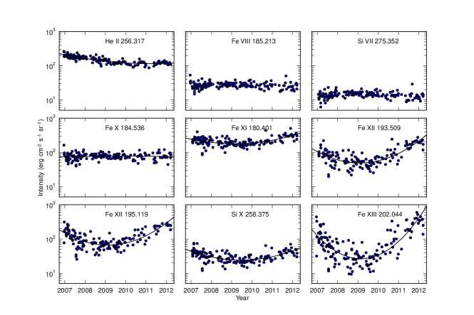
Figure 6.: Average line intensities as a function of time for the data shown in Figure fig:time-hist detrended using the fit to the Fe viii 185.213 Å and Si vii 275.352 Å intensity decays.fig:detrended-data

Following the approach used in Kamio2012, we fit the detrended data with a quadratic function to show better the behavior as a function of time. Solid lines on each panel in Figure fig:detrended-data show the results of that fitting. Using a different but very similar data set, Kamio2012 found that the hotter emission lines showed a minimum in February 2009. Our data, detrended using the newer fit obtained above, show a similar behavior. The emission lines of Fe xiii, Fe xii, and Fe xi all show a minimum in February 2009. For the Si x line, the fit has a minimum in June 2009. Note that both the cycle minimum date provided by the Space Weather Prediction Center and the results derived in Kamio2012 were obtained using data that were smoothed in time.

It is also challenging to determine how the overall solar cycle measured in the 10.7-cm radio flux or the sunspot number relates to measurements of a small region of quiet Sun. Since the activity manifestations of the solar cycle begin at high latitudes and gradually migrate toward the Equator, we would expect their effect on small regions of nominally quiet Sun near Sun center to vary. Early in the Hinode mission, the Sun was declining from its maximum in 2002. Thus much of the activity was near the Equator and we might expect some influence on EIS spectroheliograms obtained there, even for quiet regions. Activity from the new cycle, however, was initially at high latitudes. Thus, we would expect it to have a smaller impact on EIS quiet-region observations near the Equator. That impact should then grow over time.

Kamio2012 detrended their data set using an earlier sensitivity analysis that relied on the He ii 256.317 Å data that we have rejected as unsuitable. While this analysis alters the details of the time histories of the emission lines they studied, it does not alter their primary conclusion that the high-temperature component of the quiet corona changes with time, suggesting that the heat input to the quiet corona varies with time. This study further supports that conclusion.

The nature of the high-temperature emission component that overlies quiet-Sun regions and fluctuates as the solar cycle evolves has been the subject of considerable study. Vaiana1973 noted that at soft X-ray wavelengths the quiet corona consisted of large-scale structures connecting regions of opposite polarity. As the solar cycle evolves, the structures necessarily evolve as a result of the changing photospheric magnetic structure. Examining Yohkoh/Soft X-Ray Telescope observations Hara1997 noted that the quiet-Sun soft X-ray flux decreased with the decreasing magnetic flux as the solar cycle declines. Acton1999 have further quantified the behavior of the soft X-ray emission observed with that instrument. Orlando2001 examined full-disk Yohkoh/Soft X-Ray Telescope images as the solar cycle declined from 1992 to 1996. The images they present show a clear change from significant amounts of the so-called quiet corona consisting of large-scale structures near the maximum of the solar cycle to a quiet corona with significantly less large-scale overlying structure near the cycle minimum. Kamio2012 discuss further the possible energetic implications of these structural changes.

We have assumed in this analysis that the solar cycle does not affect the emission from the Fe viii and Si vii lines used to estimate the sensitivity decay constant. The lack of any significant upturn in the averaged intensities in these lines as the solar cycle rises suggests that this is the case. Continued operation of EIS through the upcoming solar maximum and beyond should help clarify the relative importance of the solar cycle in these data. If the solar cycle is lifting the intensities in the cooler lines, then the decay constant that we have derived will be an upper limit to the actual sensitivity decline. Additional insight into this issue might also be provided by examining quiet-Sun spectra in transition-region lines observed throughout the solar cycle with the Solar Ultraviolet Measurements of Emitted Radiation on the SOHO satellite [Wilhelm et al. (1995)]. Such a study, however, is beyond the scope of this article.

It is generally believed that volatiles condensing on the optical surfaces and CCDs of EIS are the most likely source of sensitivity loss (C.M. Brown, private communication, 2012). The primary absorber is then carbon. In the EIS wavelength range, a thin layer of carbon has a declining transmission as a function of wavelength [Henke, Gullikson, and Davis (1993)]. Thus we would expect the long-wavelength EIS channel to show a greater loss of sensitivity with time than the short-wavelength channel. To within the errors of the fits to the Fe viii and Si vii lines, that is not the case. The difference in transmission of a 1000 Å thick layer of carbon between 185 and 275 Å, however, is only about 15 %. Moreover, the two lines are formed at slightly different temperatures, and thus solar cycle effects could affect them differently. It may simply be that the wavelength dependence of the absorbers is masked by these effects. At some point in the future EIS will probably perform a bakeout of the CCDs to ameliorate the effect of warm and hot pixels. If that also significantly alters the sensitivity, it will add support to the idea that volatiles are the source of the sensitivity loss. Further analysis of data from well-studied ions with emission lines on both CCDs should also help to clarify this issue.

While the primary focus of this article is the decline in the sensitivity of EIS over time, it is useful to ask how the absolute intensities compare with other observations. Wang2011 have reported the results of a comparison of observations taken with a well-calibrated rocket experiment flown on 6 November 2007 and near-simultaneous EIS observations. The last two columns in Table tbl:lines list the intensities of the emission lines used in this study on the date of the rocket flight and the calibration-rocket results for the lines observed by Wang2011. The errors listed for the EIS intensities were computed by taking the standard deviation of the residuals between the model for the EIS sensitivity decline and the observed data. All of the intensities deduced using the results of this work are lower than those obtained by Wang2011. Given the very long time-constant for the EIS sensitivity decline, this suggests that the EIS prelaunch calibration may need an adjustment. A second calibration rocket in the near future may provide valuable additional insight.

Many earlier spaceborne EUV spectroscopic experiments exhibited rapid sensitivity declines. For example, the Harvard College Observatory Spectroheliometer on Skylab showed a loss of sensitivity at 977 Å of $1/e$ over a 250 day period [Reeves et al. (1977)]. The decline in sensitivity determined in this study, however, is consistent with that seen in more recent experiments such as the Coronal Diagnostic Spectrometer, which saw an overall decline in sensitivity of only about a factor of two over a 13-year period [Del Zanna et al. (2010)]. This implies a $1/e$ time of almost 19 years.

Acknowledgements

Hinode is a Japanese mission developed, launched, and operated by ISAS/JAXA in partnership with NAOJ, NASA, and STFC (UK). Additional operational support is provided by ESA and NSC (Norway). CHIANTI is a collaborative project involving the NRL (USA), the Universities of Florence (Italy) and Cambridge (UK), and George Mason University (USA). The author acknowledges support from the NASA Hinode program.

References

- Acton, Weston, and Bruner (1999) Acton, L.W., Weston, D.C., Bruner, M.E.: 1999, J. Geophys. Res. 104, 14827. doi:10.1029/1999JA900006.
- Culhane et al. (2007) Culhane, J.L., Harra, L.K., James, A.M., Al-Janabi, K., Bradley, L.J., Chaudry, R.A., Rees, K., Tandy, J.A., Thomas, P., Whillock, M.C.R., Winter, B., Doschek, G.A., Korendyke, C.M., Brown, C.M., Myers, S., Mariska, J., Seely, J., Lang, J., Kent, B.J., Shaughnessy, B.M., Young, P.R., Simnett, G.M., Castelli, C.M., Mahmoud, S., Mapson-Menard, H., Probyn, B.J., Thomas, R.J., Davila, J., Dere, K., Windt, D., Shea, J., Hagood, R., Moye, R., Hara, H., Watanabe, T., Matsuzaki, K., Kosugi, T., Hansteen, V., Wikstol, Ø.: 2007, Sol. Phys. 243, 19. doi:10.1007/s01007-007-0293-1.
- Del Zanna et al. (2010) Del Zanna, G., Andretta, V., Chamberlin, P.C., Woods, T.N., Thompson, W.T.: 2010, A&A 518, A49. doi:10.1051/0004-6361/200912904.
- Dere et al. (1997) Dere, K.P., Landi, E., Mason, H.E., Monsignori Fossi, B.C., Young, P.R.: 1997, A&AS 125, 149. doi:10.1051/aas:1997368.
- Hara (1997) Hara, H.: 1997, Advances in Space Research 20, 2279. doi:10.1016/S0273-1177(97)00901-0.
- Henke, Gullikson, and Davis (1993) Henke, B.L., Gullikson, E.M., Davis, J.C.: 1993, Atomic Data and Nuclear Data Tables 54, 181. doi:10.1006/adnd.1993.1013.
- Kamio and Mariska (2012) Kamio, S., Mariska, J.T.: 2012, Sol. Phys. 279, 419. doi:10.1007/s11207-012-0014-9.
- Korendyke et al. (2006) Korendyke, C.M., Brown, C.M., Thomas, R.J., Keyser, C., Davila, J., Hagood, R., Hara, H., Heidemann, K., James, A.M., Lang, J., Mariska, J.T., Moser, J., Moye, R., Myers, S., Probyn, B.J., Seely, J.F., Shea, J., Shepler, E., Tandy, J.: 2006, Appl. Opt. 45, 8674. doi:10.1364/AO.45.008674.
- Kosugi et al. (2007) Kosugi, T., Matsuzaki, K., Sakao, T., Shimizu, T., Sone, Y., Tachikawa, S., Hashimoto, T., Minesugi, K., Ohnishi, A., Yamada, T., Tsuneta, S., Hara, H., Ichimoto, K., Suematsu, Y., Shimojo, M., Watanabe, T., Shimada, S., Davis, J.M., Hill, L.D., Owens, J.K., Title, A.M., Culhane, J.L., Harra, L.K., Doschek, G.A., Golub, L.: 2007, Sol. Phys. 243, 3. doi:10.1007/s11207-007-9014-6.
- Landi et al. (2012) Landi, E., Del Zanna, G., Young, P.R., Dere, K.P., Mason, H.E.: 2012, ApJ 744, 99. doi:10.1088/0004-637X/744/2/99.
- Lang et al. (2006) Lang, J., Kent, B.J., Paustian, W., Brown, C.M., Keyser, C., Anderson, M.R., Case, G.C.R., Chaudry, R.A., James, A.M., Korendyke, C.M., Pike, C.D., Probyn, B.J., Rippington, D.J., Seely, J.F., Tandy, J.A., Whillock, M.C.R.: 2006, Appl. Opt. 45, 8689. doi:10.1364/AO.45.008689.
- Orlando, Peres, and Reale (2001) Orlando, S., Peres, G., Reale, F.: 2001, ApJ 560, 499. doi:10.1086/322333.
- Reeves (1976) Reeves, E.M.: 1976, Sol. Phys. 46, 53. doi:10.1007/BF00157554.
- Reeves et al. (1977) Reeves, E.M., Timothy, J.G., Withbroe, G.L., Huber, M.C.E.: 1977, Appl. Opt. 16, 849.
- Schrijver et al. (1985) Schrijver, C.J., Zwaan, C., Maxson, C.W., Noyes, R.W.: 1985, A&A 149, 123.
- Thompson (2000) Thompson, W.: 2000, Deriving statistics from nis data. CDS Software Note No. 49.
- Vaiana, Krieger, and Timothy (1973) Vaiana, G.S., Krieger, A.S., Timothy, A.F.: 1973, Sol. Phys. 32, 81. doi:10.1007/BF00152731.
- Wang et al. (2011) Wang, T., Thomas, R.J., Brosius, J.W., Young, P.R., Rabin, D.M., Davila, J.M., Del Zanna, G.: 2011, ApJS 197, 32. doi:10.1088/0067-0049/197/2/32.
- Warren (2005) Warren, H.P.: 2005, ApJS 157, 147. doi:10.1086/427171.
- Wilhelm et al. (1995) Wilhelm, K., Curdt, W., Marsch, E., Schühle, U., Lemaire, P., Gabriel, A., Vial, J.C., Grewing, M., Huber, M.C.E., Jordan, S.D., Poland, A.I., Thomas, R.J., Kühne, M., Timothy, J.G., Hassler, D.M., Siegmund, O.H.W.: 1995, Sol. Phys. 162, 189. doi:10.1007/BF00733430.