Sharp stability inequalities for planar double bubbles

Abstract.

In this paper we address the global stability problem for double-bubbles in the plane. This is accomplished by combining the improved convergence theorem for planar clusters developed in [CLM14] with an ad hoc analysis of the problem, which addresses the delicate interaction between the (possible) dislocation of singularities and the multiple-volumes constraint.

1. Introduction

The double-bubble theorem in $\mathbb{R}^{3}$ [HMRR02] asserts that the total perimeter of two regions bounding given volumes is minimized by standard double-bubbles, which are the familiar soap bubble configurations where three spherical caps meet at 120 degree angles along a circle; see Figure 1. A mathematical formulation of this result in the context of finite perimeter sets is given as follows. One says that a family $\mathcal{E}=\{\mathcal{E}(h)\}_{h=1}^{N}$ of sets of locally finite perimeter in $\mathbb{R}^{n}$ is a $N$-cluster in $\mathbb{R}^{n}$ if $|\mathcal{E}(h)|>0$ for $h=1,...,N$ and $|\mathcal{E}(h)\cap\mathcal{E}(k)|=0$ for $1\leq h<k\leq N$. We use the term double-bubble in place of $2$-cluster. Setting $\mathcal{E}(0)=\mathbb{R}^{n}\setminus\bigcup_{h=1}^{N}\mathcal{E}(h)$ for the exterior chamber of $\mathcal{E}$, one defines the perimeter and the volume of $\mathcal{E}$ as

$$P(\mathcal{E})=\frac{1}{2}\sum_{h=0}^{N}P(\mathcal{E}(h))\,,\qquad\mathrm{vol}\,(\mathcal{E})=(|\mathcal{E}(1)|,...,|\mathcal{E}(N)|)\,,$$

where $P(E)$ and $|E|$ denote, respectively, the distributional perimeter and the Lebesgue measure of a Lebesgue-measurable set $E\subset\mathbb{R}^{n}$. (In this way, $P(E)=\mathcal{H}^{n-1}(\partial E)$ whenever $E$ is an open set with Lipschitz boundary in $\mathbb{R}^{n}$, where $\mathcal{H}^{k}$ is the $k$-dimensional Hausdorff measure on $\mathbb{R}^{n}$).

For every $m_{2}\geq m_{1}>0$, there exists a unique way (up to isometries) to enclose volumes $m_{1}$ and $m_{2}$ in $\mathbb{R}^{n}$ by three $(n-1)$-dimensional spherical caps meeting at 120 degrees angles along a $(n-2)$-dimensional sphere. The corresponding shape is called the standard double-bubble in $\mathbb{R}^{n}$ (with volumes $m_{1}$ and $m_{2}$) and provides the only minimizer (up to isometries) in the isoperimetric problem

$$\inf\big{\{}P(\mathcal{E}):\mathrm{vol}\,(\mathcal{E})=(m_{1},m_{2})\big{\}}\,,\qquad m_{2}\geq m_{1}>0\,,$$ (1.1)

as shown in [FAB⁺93] when $n=2$, in [HMRR02] when $n=3$, and in [Rei08] when $n\geq 4$.

Figure 1. Standard double-bubbles: three $(n-1)$-dimensional spherical caps meeting at 120 degrees angles along a $(n-2)$-dimensional sphere (depicted by a dashed line).

In other words, if $\mathcal{E}_{0}$ denotes a generic reference standard double-bubble in $\mathbb{R}^{n}$, then

$$P(\mathcal{E})\geq P(\mathcal{E}_{0})\,,\qquad\mbox{for every double-bubble $\mathcal{E}$ with $\mathrm{vol}\,(\mathcal{E})=\mathrm{vol}\,(\mathcal{E}_{0})$}\,,$$ (1.2)

with equality if and only if $\mathcal{E}=\mathcal{E}_{0}$ modulo isometries. Our goal here is, in the planar case $n=2$, to strengthen this isoperimetric inequality in two directions. Our first result is the following sharp quantitative form of (1.2):

Theorem 1.1 (Global stability inequalities).

If $m_{2}\geq m_{1}>0$, then there exists $\kappa>0$ depending on $m_{1}$ and $m_{2}$ only such that, if $\mathcal{E}$ is a planar double-bubble with $\mathrm{vol}\,(\mathcal{E})=\mathrm{vol}\,(\mathcal{E}_{0})=(m_{1},m_{2})$, then, up to isometries,

$$P(\mathcal{E})\geq P(\mathcal{E}_{0})\Big{\{}1+\kappa\,\Big{(}|\mathcal{E}(1)\Delta\mathcal{E}_{0}(1)|+|\mathcal{E}(2)\Delta\mathcal{E}_{0}(2)|\Big{)}^{2}\Big{\}}\,.$$ (1.3)

Remark 1.1.

We stress the global character of (1.3), that is to say, $\mathcal{E}$ does not need to be a small perturbation of $\mathcal{E}_{0}$, or to be parameterized on $\mathcal{E}_{0}$ in any sense. Moreover, the decay rate in (1.3) is sharp: if $\varphi:[0,\infty)\to[0,\infty)$ is such that $P(\mathcal{E})\geq P(\mathcal{E}_{0})(1+\varphi(\sum_{i=1}^{2}|\mathcal{E}(i)\Delta\mathcal{E}_{0}(i)|))$ for every planar double-bubble $\mathcal{E}$ with $\mathrm{vol}\,(\mathcal{E})=\mathrm{vol}\,(\mathcal{E}_{0})=(m_{1},m_{2})$, then there exist $C\geq 0$ and $t_{0}>0$ such that $\varphi(t)\leq C\,t^{2}$ for every $t\leq t_{0}$; see the discussion before Theorem 2.2 below.

The typical situation in which we expect to observe double-bubbles $\mathcal{E}$ whose perimeter is close to that of a standard double-bubble $\mathcal{E}_{0}$ with $\mathrm{vol}\,(\mathcal{E}_{0})=\mathrm{vol}\,(\mathcal{E})$, is when $\mathcal{E}$ is the solution to a geometric variational problem sufficiently close to (1.1), like

$$\inf\Big{\{}P(\mathcal{E})+\beta\,\int_{\mathcal{E}(1)\cup\mathcal{E}(2)}J(x)\,dx:\mathrm{vol}\,(\mathcal{E})=(m_{1},m_{2})\Big{\}}\,,\qquad\mbox{$\beta>0$ small}\,,$$ (1.4)

where $J$ is the density of some potential energy (see also [RW13] for an account on the interaction between the cluster perimeter and a nonlocal repulsive potential). Of course one expects such minimizers to be close to standard double bubbles in a much stronger sense than the one expressed in (1.3), and we obtain such a quantitative estimate in the following theorem.

Theorem 1.2 (Perturbed minimizing clusters).

If $m_{2}\geq m_{1}>0$ and $J:\mathbb{R}^{2}\to\mathbb{R}$ is a continuous function with $J(x)\to\infty$ as $|x|\to\infty$, then there exist $C_{0}>0$ and $\beta_{0}>0$, depending on $m_{1}$, $m_{2}$, and $J$ only, with the following property. If $\mathcal{E}_{\beta}$ is a minimizer in the variational problem (1.4) with $\beta\in(0,\beta_{0})$, then there exists a standard double-bubble $\mathcal{E}_{0}$ with $\mathrm{vol}\,(\mathcal{E}_{0})=(m_{1},m_{2})$ and a $C^{1,1}$-diffeomorphism $f_{\beta}$ between $\partial\mathcal{E}_{0}$ and $\partial\mathcal{E}_{\beta}$ such that

$$\|f_{\beta}-{\rm Id}\|_{C^{0}(\partial\mathcal{E}_{0})}^{3}+\|\nabla f_{\beta}-{\rm Id}\|_{C^{0}(\partial\mathcal{E}_{0})}^{6}\leq C_{0}\,\beta\,.$$

We now comment on the related literature on quantitative isoperimetric inequalities, and on the strategy of proof of our main results. After the pioneering contributions by Bernstein [Ber05] and Bonnesen [Bon24], the analysis of global stability problems has received a renewed attention in recent years, with the proof of the sharp stability inequality for the Euclidean isoperimetric problem [Fug89, Fug93, HHW91, Hal92, FMP08, CL12, FGP12, FJ14], the Wulff isoperimetric problem [FMP10], the Gaussian isoperimetric problem [CFMP11, MN15, BBJ14], Plateau-type problems [DPM14], fractional isoperimetric problems [FMM11], and isoperimetric problems in higher codimension [BDF12]. (This list is probably incomplete, and it does not mention contributions to stability problems for functional inequalities.)

Among the various methods developed to deal with global stability problems in the above mentioned papers, the selection principle method from [CL12] has proven to be the more widely applicable. At the heart of this approach lies the use of regularity theory to obtain what we call improved convergence theorems. Referring to the introduction of [CLM14] for a more detailed account on this kind of results, we just notice here that by exploiting the main result from [CLM14] in combination with a selection principle we can reduce the proof of (1.3) to the case when $\partial\mathcal{E}=f(\partial\mathcal{E}_{0})$ for a $C^{1,1}$-diffeomorphism $f$ between $\partial\mathcal{E}_{0}$ and $\partial\mathcal{E}$ such that $\|f-{\rm Id}\|_{C^{1}(\partial\mathcal{E}_{0})}$ is as small as needed. In the case of the standard isoperimetric problem, following Fuglede [Fug89, Fug93], one can directly address this “reduced” stability problem by an expansion in spherical harmonics, which is elementary if $n=2$.

In the case of double-bubbles, even when $n=2$, the situation is much subtler, due to the presence of singularities and of the multiple-volumes constraint. We shall address this problem by combining Fourier series arguments in the spirit of Fuglede with the solution of certain one-dimensional variational problems, to proceed through a case by case analysis. Different cases will correspond to different behaviors of the perturbed interfaces, based for example on the relative size between their $L^{2}$-mean deviation and their $L^{2}$-distance from the corresponding interfaces of the reference standard double-bubble. The resulting argument, although based on rather elementary mathematical tools, sheds light on the non-trivial interactions between the three interfaces, on which the global stability of standard double-bubbles ultimately depends. As an entirely analogous structure underlies the stability problem for standard double-bubbles in higher dimensions, we expect the methods of this paper to be useful also in that case.

We notice that, at present, there is only another instance of isoperimetric problem with multiple volume constraints whose minimizers are explicitly known. This is the case of the planar triple bubble problem, addressed by Wichiramala in [Wic04]. It is reasonable to expect that by further exploiting the arguments developed in this paper, and again in combination with the improved convergence theorem from [CLM14], one should be able to obtain results like Theorem 1.1 and Theorem 1.2 in the case of planar triple bubbles too.

The paper is organized as follows. In section 2 we reduce the proof of Theorem 1.1 to the case of small diffeomorphic images of $\mathcal{E}_{0}$. In section 3 we introduce the notion of $(\varepsilon,\sigma)$-perturbation of a standard double-bubble, and prove Theorem 1.1 and Theorem 1.2 assuming Theorem 1.1 on $(\varepsilon,\sigma)$-perturbations. Finally, in section 4, we address the proof of Theorem 1.1 on $(\varepsilon,\sigma)$-perturbations.

Acknowledgements

GPL is supported by the GNAMPA-INdAM project Problemi di regolarità e teoria geometrica della misura in spazi metrici and by the PRIN 2010 M.I.U.R. project Calcolo delle Variazioni. FM is supported by NSF-DMS Grant 1265910 and NSF-DMS FRG Grant 1361122.

2. Reduction to small perturbations

2.1. Sets of finite perimeter, clusters, and improved convergence

We describe bubble clusters in the framework of the theory of sets of finite perimeter. Referring to [Mag12] for more details, given a set $E$ of locally finite perimeter in $\mathbb{R}^{n}$, we denote by $\mu_{E}=\nu_{E}\,\mathcal{H}^{n-1}\llcorner\partial^{*}E$ its Gauss–Green measure, where $\nu_{E}$ and $\partial^{*}E$ are the measure-theoretic outer unit normal and the reduced boundary of $E$, respectively. In this way the perimeter of $E$ relative to the Borel set $F$ is $P(E;F)=|\mu_{E}|(F)=\mathcal{H}^{n-1}(F\cap\partial^{*}E)$, and we set $P(E)=P(E;\mathbb{R}^{n})$. We work under the normalization by a Lebesgue negligible set which ensures that

$$\overline{\partial^{*}E}={\rm spt}\,\mu_{E}=\big{\{}x\in A:0<|E\cap B_{x,r}|<\omega_{n}\,r^{n}\quad\forall r>0\big{\}}=\partial E\,,$$

Given a $N$-cluster $\mathcal{E}$ in $\mathbb{R}^{n}$, we set

$$\partial^{*}\mathcal{E}=\bigcup_{h=1}^{N}\partial^{*}\mathcal{E}(h)\,,\qquad\partial\mathcal{E}=\bigcup_{h=1}^{N}\partial\mathcal{E}(h)\,,\qquad\Sigma(\mathcal{E})=\partial\mathcal{E}\setminus\partial^{*}\mathcal{E}\,,$$

so that $\overline{\partial^{*}\mathcal{E}}=\partial\mathcal{E}$. We set $\mathrm{d}(\mathcal{E},\mathcal{F})=(1/2)\,\sum_{h=0}^{N}|\mathcal{E}(h)\Delta\mathcal{F}(h)|$ for the $L^{1}$-distance between the $N$-clusters $\mathcal{E}$ and $\mathcal{F}$, and say that $\mathcal{E}$ is a $(\Lambda,r_{0})$-minimizing cluster in $\mathbb{R}^{n}$ if

$$P(\mathcal{E})\leq P(\mathcal{F})+\Lambda\,\mathrm{d}(\mathcal{E},\mathcal{F})\,,$$ (2.1)

whenever $\mathcal{E}(h)\Delta\mathcal{F}(h)\subset\subset B_{x,r_{0}}$ for some $x\in\mathbb{R}^{n}$ and every $h=1,...,N$. Referring to [CLM14, Section 4] for an account on the regularity properties of $(\Lambda,r_{0})$-minimizing clusters in $\mathbb{R}^{n}$ for $n$ arbitrary, here we just need to recall what happens when $n=2$. Let us say that $\mathcal{E}$ is a $C^{k,\alpha}$-cluster in $\mathbb{R}^{2}$ ($k\in\mathbb{N}$, $\alpha\in(0,1]$) if there exist a locally finite family $\{\gamma_{i}\}_{i\in I}$ of closed $C^{k,\alpha}$-curves with boundary in $\mathbb{R}^{2}$ and a locally finite family of points $\{p_{j}\}_{j\in J}$ such that

$$\partial\mathcal{E}=\bigcup_{i\in I}\gamma_{i}\,,\qquad\partial^{*}\mathcal{E}=\bigcup_{i\in I}{\rm int}\,(\gamma_{i})\,,\qquad\Sigma(\mathcal{E})=\bigcup_{i\in I}{\rm bd}\,(\gamma_{i})=\bigcup_{j\in J}\{p_{j}\}\,,$$

where ${\rm int}\,(\gamma)$ and ${\rm bd}\,(\gamma)$ denote the interior and the boundary points of the curve $\gamma$. If $\mathcal{E}$ is a $(\Lambda,r_{0})$-minimizing cluster in $\mathbb{R}^{2}$ then $\mathcal{E}$ is a $C^{1,1}$-cluster in $\mathbb{R}^{2}$: moreover, each $\gamma_{i}$ to have distributional curvature bounded by $\Lambda$, and each $p_{j}$ to be a boundary point of exactly three curves from $\{\gamma_{i}\}_{i\in I}$, which form three 120 degrees angles at $p_{j}$. For a proof of all these facts we refer, for example, to [CLM14, Theorem 5.2].

Given a $C^{1,1}$-cluster $\mathcal{E}$ in $\mathbb{R}^{2}$ and a map $f:\partial\mathcal{E}\to\mathbb{R}^{2}$ one says that $f\in C^{1,1}(\partial\mathcal{E};\mathbb{R}^{2})$ if $f$ is continuous on $\partial\mathcal{E}$ and

$$\|f\|_{C^{1,1}(\partial\mathcal{E})}:=\sup_{i\in I}\|f\|_{C^{1,1}(\gamma_{i})}<\infty\,;$$

moreover, given $C^{1,1}$-clusters $\mathcal{E}$ and $\mathcal{F}$, one says that $f$ is a $C^{1,1}$-diffeomorphism between $\partial\mathcal{E}$ and $\partial\mathcal{F}$ if $f$ is an homeomorphism between $\partial\mathcal{E}$ and $\partial\mathcal{F}$ with $f\in C^{1,1}(\partial\mathcal{E};\mathbb{R}^{2})$, $f^{-1}\in C^{1,1}(\partial\mathcal{F};\mathbb{R}^{2})$ and $f(\Sigma(\mathcal{E}))=\Sigma(\mathcal{F})$. Finally, given a map $f:\partial\mathcal{E}\to\mathbb{R}^{2}$, and denoted by $\nu:\partial^{*}\mathcal{E}\to S^{1}$ a vector field with $\nu(x)\in\{\nu_{\mathcal{E}(h)}(x),\nu_{\mathcal{E}(k)}(x)\}$ for every $x\in\partial^{*}\mathcal{E}(h)\cap\partial^{*}\mathcal{E}(k)$, we define the tangential component $\boldsymbol{\tau}_{\mathcal{E}}:\partial^{*}\mathcal{E}\to\mathbb{R}^{2}$ of $f$ with respect to $\mathcal{E}$ by setting

$$\boldsymbol{\tau}_{\mathcal{E}}f(x)=f(x)-(f(x)\cdot\nu(x))\nu(x)\qquad x\in\partial^{*}\mathcal{E}\,.$$

(Note that the continuity of $\nu$ is not essential here, as $\boldsymbol{\tau}_{\mathcal{E}}f$ depends quadratically from $\nu$.) The following result is [CLM14, Theorem 1.5].

Theorem 2.1.

Given $\Lambda\geq 0$, $r_{0}>0$ and a bounded $C^{2,1}$-cluster $\mathcal{E}_{0}$ in $\mathbb{R}^{2}$, there exist positive constants $\mu_{0}$ and $C_{0}$ (depending on $\Lambda$ and $\mathcal{E}$) with the following property.

If $\{\mathcal{E}_{k}\}_{k\in\mathbb{N}}$ is a sequence of $(\Lambda,r_{0})$-minimizing clusters in $\mathbb{R}^{2}$ such that $\mathrm{d}(\mathcal{E}_{k},\mathcal{E}_{0})\to 0$ as $k\to\infty$, then for every $\mu<\mu_{0}$ there exist $k(\mu)\in\mathbb{N}$ and a sequence of maps $\{f_{k}\}_{k\geq k(\mu)}$ such that each $f_{k}$ is a $C^{1,1}$-diffeomorphism between $\partial\mathcal{E}_{0}$ and $\partial\mathcal{E}_{k}$ with

$$\|f_{k}\|_{C^{1,1}(\partial\mathcal{E}_{0})} \leq C_{0}\,,$$ (2.2)

$$\lim_{k\to\infty}\|f_{k}-{\rm Id}\|_{C^{1}(\partial\mathcal{E}_{0})} = 0\,,$$ (2.3)

$$\boldsymbol{\tau}_{\mathcal{E}_{0}}(f_{k}-{\rm Id}) = 0\,,\qquad\mbox{on $\partial\mathcal{E}_{0}\setminus I_{\mu}(\Sigma(\mathcal{E}_{0}))$}\,,$$ (2.4)

$$\|\boldsymbol{\tau}_{\mathcal{E}_{0}}(f_{k}-{\rm Id})\|_{C^{1}(\partial^{*}\mathcal{E}_{0})} \leq \frac{C_{0}}{\mu}\,\|f_{k}-{\rm Id}\|_{C^{0}(\Sigma(\mathcal{E}_{0}))}\,.$$ (2.5)

2.2. A selection principle

Let now $\mathcal{E}_{0}$ denote a reference standard double-bubble in $\mathbb{R}^{2}$ with $\mathrm{vol}\,(\mathcal{E}_{0})=(m_{1},m_{2})$, and for every planar double-bubble $\mathcal{E}$ set

$$\delta(\mathcal{E})=P(\mathcal{E})-P(\mathcal{E}_{0})\,,$$

$$\alpha(\mathcal{E})=\inf\big{\{}\mathrm{d}(\mathcal{E},f(\mathcal{E}_{0})):\mbox{$f:\mathbb{R}^{2}\to\mathbb{R}^{2}$ is an isometry}\big{\}}\,,$$

and

$$\kappa(\mathcal{E}_{0})=\inf\big{\{}\liminf_{k\to\infty}\frac{\delta(\mathcal{E}_{k})}{\alpha(\mathcal{E}_{k})^{2}}:\mathrm{vol}\,(\mathcal{E}_{k})=(m_{1},m_{2})\,,\alpha(\mathcal{E}_{k})>0\,,\lim_{k\to\infty}\mathrm{d}(\mathcal{E}_{k},\mathcal{E}_{0})=0\big{\}}\,.$$ (2.6)

Notice that, by pushing the interfaces of $\mathcal{E}_{0}$ as depicted in Figure 2,

Figure 2. The deformations $\mathcal{E}_{t}$ of $\mathcal{E}_{0}$ used to prove that $\kappa(\mathcal{E}_{0})<\infty$ is depicted on the right.

one defines a one-parameter family of double-bubbles $\{\mathcal{E}_{t}\}_{0<t<1}$ such that

$$\mathrm{vol}\,(\mathcal{E}_{t})=\mathrm{vol}\,(\mathcal{E}_{0})\,,\qquad P(\mathcal{E}_{t})\leq P(\mathcal{E}_{0})+C\,t^{2}\,,\qquad\mathrm{d}(\mathcal{E}_{t},\mathcal{E}_{0})\geq C\,t\,,\qquad\forall t\in(0,1)\,;$$

moreover, by exploiting the symmetry of $\mathcal{E}_{t}$ (see [Mag08, Lemma 5.2] for the kind of argument used here) one has

$$\mathrm{d}(\mathcal{E}_{t},\mathcal{E}_{0})\leq C\,\alpha(\mathcal{E}_{t})\,,\qquad\forall t\in(0,1)\,,$$

so that $\kappa(\mathcal{E}_{0})<\infty$. This last fact shows, in particular, the sharpness of the decay rate in (1.3) claimed in Remark 1.1. Now, Theorem 1.1 is equivalent to $\kappa(\mathcal{E}_{0})>0$, and Theorem 2.2 below allows one to reduce the proof of Theorem 1.1 to the case when $\partial\mathcal{E}$ is a $C^{1,1}$-diffeomorphic image of $\partial\mathcal{E}_{0}$ (in the sense of Theorem 2.1) by a map $f$ that is arbitrarily $C^{1}$-close to the identity.

Theorem 2.2.

There exist positive constants $C_{0}$ and $\mu_{0}$ (depending on $m_{1}$ and $m_{2}$ only) and a sequence of planar double-bubbles $\{\mathcal{E}_{k}\}_{k\in\mathbb{N}}$ with $\mathrm{vol}\,(\mathcal{E}_{k})=(m_{1},m_{2})$, such that

$$\inf_{k\in\mathbb{N}}\alpha(\mathcal{E}_{k})>0\,,\qquad\lim_{k\to\infty}\mathrm{d}(\mathcal{E}_{k},\mathcal{E}_{0})=0\,,\qquad\lim_{k\to\infty}\frac{\delta(\mathcal{E}_{k})}{\alpha(\mathcal{E}_{k})^{2}}=\kappa(\mathcal{E}_{0})\,,$$ (2.7)

and such that for every $\mu\in(0,\mu_{0})$ there exist $k(\mu)\in\mathbb{N}$ and, for each $k\geq k(\mu)$, a $C^{1,1}$-diffeomorphism $f_{k}$ between $\partial\mathcal{E}_{0}$ and $\partial\mathcal{E}_{k}$, in such a way that (2.2)–(2.5) hold.

Proof.

By Theorem A.2 in Appendix A there exists a sequence $\{\mathcal{E}_{k}\}_{k\in\mathbb{N}}$ of $(\Lambda,r_{0})$-minimizing $2$-clusters in $\mathbb{R}^{2}$ with $\mathrm{vol}\,(\mathcal{E}_{k})=(m_{1},m_{2})$ satisfying (2.7). Since $\mathrm{d}(\mathcal{E}_{k},\mathcal{E}_{0})\to 0$, by applying Theorem 2.1 we find diffeomorphisms $f_{k}$ between $\partial\mathcal{E}_{0}$ and $\partial\mathcal{E}_{k}$ with the required properties. ∎

3. Proofs of the main theorems

Given $\varepsilon>0$ and $\sigma\in(-1,1)$, and denoted by $\nu_{\mathcal{E}_{0}}$ a normal vector field to $\partial^{*}\mathcal{E}_{0}$, one says that a planar double-bubble $\mathcal{E}$ is an $(\varepsilon,\sigma)$-perturbation of $\mathcal{E}_{0}$ if $\mathrm{vol}\,(\mathcal{E})=\mathrm{vol}\,(\mathcal{E}_{0})$ and there exist $g\in C^{1}(\partial\mathcal{E}_{0};\mathbb{R}^{2})$ with

$$g={\rm Id}\quad\mbox{on $\Sigma(\mathcal{E}_{0})$}\,,\qquad(g-{\rm Id})\cdot\nu_{\mathcal{E}_{0}}=0\quad\mbox{on $\partial^{*}\mathcal{E}_{0}$}\,,\qquad\|g-{\rm Id}\|_{C^{1}(\partial\mathcal{E}_{0})}<\varepsilon\,,$$ (3.1)

and such that $\partial\mathcal{E}=(1+\sigma)\,g(\partial\mathcal{E}_{0})$. In the next section, see Theorem 4.7, we show the existence of positive constants $\varepsilon_{1}$ and $\sigma_{1}$ such that (1.3) hold on every $(\varepsilon,\sigma)$-perturbation of $\mathcal{E}_{0}$ with $\varepsilon<\varepsilon_{1}$ and $|\sigma|<\sigma_{1}$. Based on Theorem 2.2 and Theorem 4.7 one can prove Theorem 1.1 as follows.

Proof of Theorem 1.1.

By Theorem 2.2 and Theorem 4.7 it suffices to show that if $\{\mathcal{E}_{k}\}_{k\in\mathbb{N}}$ is a sequence of $(\Lambda,r_{0})$-minimizing clusters such that $\mathrm{d}(\mathcal{E}_{k},\mathcal{E}_{0})\to 0$, then for every $k$ large enough $\mathcal{E}_{k}$ is an $(\varepsilon_{k},\sigma_{k})$-perturbation of $\mathcal{E}_{0}$, where $\varepsilon_{k},\sigma_{k}\to 0$ as $k\to\infty$. In other words, we want to prove that, up to isometries, $\partial\mathcal{E}_{k}$ is a $C^{1}$-small normal perturbation of the small rescaling $(1+\sigma_{k})\partial\mathcal{E}_{0}$ of $\partial\mathcal{E}_{0}$.

We already know $\partial\mathcal{E}_{k}$ to be a $C^{1}$-small perturbation of $\partial\mathcal{E}_{0}$ with a small tangential displacement. Indeed, if $C_{0}$ and $\mu_{0}$ are as in Theorem 2.1, then by Theorem 2.2 and for every $\mu<\mu_{0}$ we find $\{f_{k}\}_{k\geq k(\mu)}$ (the dependence of $f_{k}$ from $\mu$ is tacitly understood) such that (2.2)–(2.5) hold. We now exploit the existence of the maps $f_{k}$ to show that (3.1) holds with $\mathcal{E}=\mathcal{E}_{k}$ for some $\sigma=\sigma_{k}\to 0$, $\varepsilon=\varepsilon_{k}\to 0$ and $g=g_{k}$.

Let us set $\Sigma(\mathcal{E}_{0})=\{p_{1},p_{2}\}$ and let $\{\gamma_{i}\}_{i=1}^{3}$ be the circular arcs such that $\partial\mathcal{E}_{0}=\bigcup_{i=1}^{3}\gamma_{i}$ and ${\rm bd}\,(\gamma_{i})=\{p_{1},p_{2}\}$ for $i=1,2,3$. Up to a translation of $\mathcal{E}_{0}$ (and, correspondingly, of each $\mathcal{E}_{k}$) we may assume that $p_{1}+p_{2}=0$. Setting $p_{j}^{k}=f_{k}(p_{j}^{k})$, we have $\Sigma(\mathcal{E}_{k})=\{p_{1}^{k},p_{2}^{k}\}$ and $p_{j}^{k}\to p_{j}$ by (2.3), so that, up to moving each $\mathcal{E}_{k}$ by an isometry (with the corresponding sequence of isometries which converges to the identity map) we entail

$$p_{j}^{k}=(1+\sigma_{k})\,p_{j}\,,\qquad\lim_{k\to\infty}\sigma_{k}=0\,.$$ (3.2)

If we set $\gamma_{i}^{k}=(1+\sigma_{k})^{-1}\,f_{k}(\gamma_{i})$, then

$$(1+\sigma_{k})^{-1}\partial\mathcal{E}_{k}=\bigcup_{i=1}^{3}\gamma_{i}^{k}\,,\qquad{\rm bd}\,(\gamma_{i}^{k})=\{p_{1},p_{2}\}\,.$$

Thanks to (2.2)–(2.5), by $\gamma_{i}^{k}=(1+\sigma_{k})^{-1}\,f_{k}(\gamma_{i})$, and since $\sigma_{k}\to 0$, one has:

(i) if $\tau_{\gamma}:{\rm bd}\,(\gamma)\to S^{1}$ is the outer unit tangent vector to a curve $\gamma$ at its boundary points, then

$$\lim_{k\to\infty}\mathrm{hd}(\gamma_{i}^{k},\gamma_{i})+\max_{j=1,2}|\tau_{\gamma_{i}^{k}}(p_{j})-\tau_{\gamma_{i}}(p_{j})|=0\,;$$

moreover, by exploiting the fact that $f_{k}$ parameterizes $\gamma_{i}^{k}$ over $\gamma_{i}$, one constructs unit normal vector fields $\nu_{i}^{k}\in C^{0,1}(\gamma_{i}^{k};S^{1})$ to $\gamma_{i}^{k}$ such that

$$|\nu_{i}^{k}(x)\cdot(y-x)|\leq L\,|x-y|^{2}\,,\qquad|\nu_{i}^{k}(x)-\nu_{i}^{k}(y)|\leq L\,|x-y|\,,\qquad\forall x,y\in\gamma_{i}^{k}\,,$$

where $L$ is independent from $k$;

(ii) if we set $[\gamma_{i}]_{t}=\{x\in\gamma_{i}:\hbox{dist}(x,{\rm bd}\,(\gamma_{i}))>t\}$, $t>0$, and $\psi_{k}=(1+\sigma_{k})^{-1}\,(f_{k}-{\rm Id})\cdot\nu_{i}$, then $\psi_{k}\in C^{1,1}([\gamma_{i}]_{\mu})$ for every $i=1,2,3$ with

$$\sup_{k\geq k(\mu)}\|\psi_{k}\|_{C^{1,1}([\gamma_{i}]_{\mu})}\leq C_{0}\,,\qquad\lim_{k\to\infty}\|\psi_{k}\|_{C^{1}([\gamma_{i}]_{\mu})}=0\,,$$

$$[\gamma_{i}^{k}]_{2\mu}\subset({\rm Id}+\psi_{k}\nu_{i})([\gamma_{i}]_{\mu})\subset\gamma_{i}^{k}\,,$$

where $\nu_{i}\in C^{0,1}(\gamma_{i};S^{1})$ is a fixed outer unit normal to $\gamma_{i}$.

Thanks to (i) and (ii) we can apply [CLM14, Theorem 3.5] to construct a $C^{1,1}$-normal diffeomorphism $\hat{g}_{i}^{k}$ between $\gamma_{i}$ and $\gamma_{i}^{k}$ such that $\hat{g}_{i}^{k}\to{\rm Id}$ in $C^{1}(\gamma_{i})$. Note that, in fact, $\hat{g}_{i}^{k}$ is a normal diffeomorphism as ${\rm bd}\,(\gamma_{i})={\rm bd}\,(\gamma_{i}^{k})$, cf. with [CLM14, Equation (3.85)]. Setting $g_{k}=\hat{g}_{i}^{k}$ on $\gamma_{i}$, we thus define a normal $C^{1,1}$-diffeomorphism between $\partial\mathcal{E}_{0}$ and $(1+\sigma_{k})^{-1}\partial\mathcal{E}_{k}$ with $\varepsilon_{k}=\|g_{k}-{\rm Id}\|_{C^{1}(\partial\mathcal{E}_{0})}\to 0$. ∎

Proof of Theorem 1.2.

We directly focus on the case $m_{2}>m_{1}$, the case $m_{2}=m_{1}$ being analogous. Let us pick an arbitrary sequence $\beta_{k}\to 0^{+}$, and let $\mathcal{E}_{k}$ be minimizers in (1.4) with $\beta=\beta_{k}$. By arguing as in [CLM14, Proof of Theorem 1.10] we prove the existence of $\Lambda\geq 0$ and $r_{0}>0$ such that $\{\mathcal{E}_{k}\}_{k\in\mathbb{N}}$ is a sequence of $(\Lambda,r_{0})$-minimizers such that, up to isometries, $\mathrm{d}(\mathcal{E}_{k},\mathcal{E}_{0})\to 0$. By the argument used to prove Theorem 1.1, we see that $\mathcal{E}_{k}$ is an $(\varepsilon_{k},\sigma_{k})$-perturbation of $\mathcal{E}_{0}$ with $\varepsilon_{k},\sigma_{k}\to 0$. As a first consequence, we note that if $R>0$ is such that $\mathcal{E}_{0}(h)\subset B_{R}$ for $h=1,2$, then for $k$ large enough $\mathcal{E}_{k}(h)\subset B_{2R}$ for $h=1,2$, and thus by minimality of $\mathcal{E}_{k}$,

$$P(\mathcal{E}_{k})-P(\mathcal{E}_{0})\leq C\,\beta_{k}\,\|J\|_{C^{0}(B_{2R})}\,\sum_{h=1}^{2}\,|\mathcal{E}_{k}(h)\Delta\mathcal{E}_{0}(h)|\leq C\,\beta_{k}\,.$$

At the same time, if with the same notation of the previous proof we denote by $\{\gamma_{i}\}_{i=0}^{2}$ the circular arcs composing $\partial\mathcal{E}_{0}$, then there exist $u_{k,i}\in C^{1,1}_{0}(\gamma_{i})$ such that

$$\lim_{k\to\infty}\|u_{k,i}\|_{C^{1}(\gamma_{i})}=0\,,\qquad\sup_{k\in\mathbb{N}}\|u_{k,i}^{\prime\prime}\|_{L^{\infty}(\gamma_{i})}\leq\Lambda\,,\qquad\forall i=0,1,2\,,$$ (3.3)

and such that, by setting

$$\bar{g}_{k}(x)=(1+\sigma_{k})\,\big{(}x+u_{k,i}(x)\,\nu_{i}(x)\big{)}\,,\qquad x\in\gamma_{i}\,,$$

one defines a $C^{1,1}$-diffeomorphism $\bar{g}_{k}$ between $\partial\mathcal{E}_{0}$ and $\partial\mathcal{E}_{k}$ with

$$\|\bar{g}_{k}-{\rm Id}\|_{C^{j}(\partial\mathcal{E}_{0})}\leq C\,\Big{(}|\sigma_{k}|+\sum_{i=0}^{2}\|u_{k,i}\|_{C^{j}(\gamma_{i})}\Big{)}\,,\qquad j=1,2\,,$$ (3.4)

Since $\varepsilon_{k},\sigma_{k}\to 0$, for $k$ large enough we can use Theorem 4.7 to deduce that

$$P(\mathcal{E}_{k})-P(\mathcal{E}_{0})\geq\kappa\,\Big{(}\sigma_{k}^{2}+\sum_{i=0}^{2}\int_{\gamma_{i}}\,u_{k,i}^{2}\Big{)}\,,$$ (3.5)

and then apply Lemma 3.1 below to get

$$\|\bar{g}_{k}-{\rm Id}\|_{C^{0}(\partial\mathcal{E}_{0})}^{3}+\|\nabla\bar{g}_{k}-{\rm Id}\|_{C^{0}(\partial\mathcal{E}_{0})}^{6}\leq C\,\beta_{k}\,.$$

By the arbitrariness of $\beta_{k}$ we conclude the proof of the theorem. ∎

Lemma 3.1.

If $v\in C^{1,1}([a,b])$ with $v(a)=v(b)=0$, then

$$\begin{split}C\,\|v\|_{L^{1}(a,b)}^{2/3}\,\|v^{\prime\prime}\|_{L^{\infty}(a,b)}^{1/3}\geq\|v\|_{C^{0}([a,b])}\,,\\ C\,\|v\|_{L^{1}(a,b)}^{1/3}\,\|v^{\prime\prime}\|_{L^{\infty}(a,b)}^{2/3}\geq\|v^{\prime}\|_{C^{0}([a,b])}\,.\end{split}$$ (3.6)

Proof.

The argument is elementary and it is included just for the sake of clarity. Without loss of generality, let $x_{0}\in(a,b)$ be such that $\|v\|_{C^{0}([a,b])}=|v(x_{0})|=v(x_{0})>0$. Since $v(b)=0$, there exists $\bar{x}\in(x_{0},b]$ such that $v>0$ on $(x_{0},\bar{x})$ and $v(\bar{x})=0$. By $v^{\prime}(x_{0})=0$ we find

$$|v(x)|=v(x)\geq v(x_{0})-\frac{\|v^{\prime\prime}\|_{L^{\infty}(a,b)}}{2}(x-x_{0})^{2}\,,\qquad\forall x\in(x_{0},\bar{x})\,.$$

The right-hand side of this inequality is positive for $x\in(x_{0},x_{0}+r)$ where

$$r=\Big{(}\frac{2\|v\|_{C^{0}([a,b])}}{\|v^{\prime\prime}\|_{L^{\infty}(a,b)}}\Big{)}^{1/2}\,,$$

hence $(x_{0},x_{0}+r)\subset(x_{0},\bar{x})$, and thus

$$\|v\|_{L^{1}(a,b)}\geq\int_{(x_{0},x_{0}+r)}\Big{(}v(x_{0})-\frac{\|v^{\prime\prime}\|_{L^{\infty}(a,b)}}{2}(x-x_{0})^{2}\Big{)}\,dx=\frac{2\sqrt{2}}{3}\,\frac{\|v\|_{C^{0}([a,b])}^{3/2}}{\|v^{\prime\prime}\|_{L^{\infty}(a,b)}^{1/2}}\,.$$

which is the first estimate in (3.6). Now we take $x_{1}\in[a,b]$ such that $|v^{\prime}(x_{1})|=\|v^{\prime}\|_{C^{0}([a,b])}$. Without loss of generality we can assume that $|v^{\prime}(x_{1})|=v^{\prime}(x_{1})>0$ and that $v(x_{1})\geq 0$. (Indeed, this can be achieved by possibly replacing $v$ with $-v$ and then by reflecting $v$ with respect to the mid-point of $[a,b]$. Notice that this operation may in principle change the sign of $v(x_{0})$, but this will not affect our argument as we shall not need to refer to $v(x_{0})$ anymore.) Since $v(b)=0$, there exists $x_{2}\in(x_{1},b)$ such that $v^{\prime}=|v^{\prime}|>0$ on $(x_{1},x_{2})$ and $v^{\prime}(x_{2})=0$, and thus, by $v(x_{1})\geq 0$, $|v|=v$ on $(x_{1},x_{2})$. In particular,

$$|v(x)| = v(x)\geq v(x_{1})+v^{\prime}(x_{1})(x-x_{1})-\frac{\|v^{\prime\prime}\|_{L^{\infty}(a,b)}}{2}\,|x-x_{1}|^{2}$$

$$\geq v^{\prime}(x_{1})(x-x_{1})-\frac{\|v^{\prime\prime}\|_{L^{\infty}(a,b)}}{2}\,|x-x_{1}|^{2}\,,\qquad\forall x\in(x_{1},x_{2})\,,$$

where the right-hand side of this inequality is non-negative for $x\in(x_{1},x_{1}+s)$, where

$$s=\frac{2\|v^{\prime}\|_{C^{0}([a,b])}}{\|v^{\prime\prime}\|_{L^{\infty}(a,b)}}\,.$$

In particular $(x_{1},x_{1}+s)\subset(x_{1},x_{2})$, and thus

$$\|v\|_{L^{1}(a,b)}\geq\int_{(x_{1},x_{1}+s)}\Big{(}v^{\prime}(x_{1})(x-x_{1})-\frac{\|v^{\prime\prime}\|_{L^{\infty}(a,b)}}{2}\,|x-x_{1}|^{2}\Big{)}\,dx=\frac{2}{3}\,\frac{\|v^{\prime}\|_{C^{0}([a,b])}^{3}}{\|v^{\prime\prime}\|_{L^{\infty}(a,b)}^{2}}\,.$$

∎

4. Stability on $(\varepsilon,\sigma)$-perturbations

We now turn to the proof of Theorem 1.1 on $(\varepsilon,\sigma)$-perturbations of $\mathcal{E}_{0}$, see Theorem 4.7 below. We begin by introducing some specific notation for spherical caps and sectors, and for their normal perturbation by a given function. Let $B=\{x\in\mathbb{R}^{2}:|x|<1\}$. Given $\theta\in(0,\pi)$, we define a circular arc $A(\theta)\subset\partial B$ and a circular sector $S(\theta)\subset B$ by setting

$$A(\theta)=\big{\{}x\in\mathbb{R}^{2}:|x|=1\,,x_{1}>\cos\theta\big{\}}\,,\qquad S(\theta)=\big{\{}t\,x:x\in A(\theta)\,,0<t<1\big{\}}\,,$$

while, given $u\in W^{1,2}_{0}(A(\theta))$ we denote by $A(\theta,u)\subset\mathbb{R}^{2}$ and $S(\theta,u)\subset\mathbb{R}^{2}$ the perturbed circular arc and perturbed circular sector defined as

$$A(\theta,u)=\big{\{}(1+u(x))\,x:x\in A(\theta)\big{\}}\,,\qquad S(\theta,u)=\big{\{}t\,(1+u(x))\,x:x\in A(\theta)\,,0<t<1\big{\}}\,;$$

see Figure 3.

Figure 3. The circular arc $A(\theta)$, the circular sector $S(\theta)$, and their perturbations defined by $u\in W^{1,2}_{0}(A(\theta))$.

(Notice that $A(\theta,0)=A(\theta)$ and $S(\theta,0)=S(\theta)$.) In the analysis of the case $m_{1}=m_{2}$, where the interface between the chambers is a segment, it is convenient to introduce as a reference domain the vertical open segment $H$ and its perturbations $H(u)$ defined as

$$H=\big{\{}x\in\mathbb{R}^{2}:\,|x_{2}|<\frac{\sqrt{3}}{2},\,x_{1}=0\big{\}}\,,\qquad H(u)=\big{\{}x+u(x)\,e_{1}:x\in\,H\big{\}}\,,$$ (4.1)

in correspondence of $u\in W^{1,2}_{0}(H)$. We occasionally identify $A(\theta)$ with the interval $(-\theta,\theta)$ and $H$ with the interval $(-\sqrt{3}/2,\sqrt{3}/2)$; correspondingly, we identify $W_{0}^{1,2}(A(\theta))$ with $W_{0}^{1,2}(-\theta,\theta)$ and $W^{1,2}_{0}(H)$ with $W^{1,2}_{0}(-\sqrt{3}/2,\sqrt{3}/2)$.

Lemma 4.1.

If $u\in C^{1}_{0}(-\theta,\theta)$, then

$$|S(\theta,u)|-|S(\theta)| = \int_{-\theta}^{\theta}u+\frac{u^{2}}{2}\,,$$ (4.2)

$$\mathcal{H}^{1}(A(\theta,u))-\mathcal{H}^{1}(A(\theta)) = \int_{-\theta}^{\theta}u+\frac{(u^{\prime})^{2}}{2}\,+\|u\|_{C^{1}(-\theta,\theta)}\,{\mathrm{O}}(\|u\|_{W^{1,2}(-\theta,\theta)}^{2})\,.\hskip 14.22636pt$$ (4.3)

Moreover, if $|u|\leq 1$, then

$$|S(\theta,u)\Delta S(\theta)|\leq\frac{3}{2}\,\int_{-\theta}^{\theta}|u|\,.$$ (4.4)

Proof.

Identity (4.2) follows from $|S(\theta,u)|=(1/2)\int_{-\theta}^{\theta}(1+u)^{2}$, which also implies (4.4) since, if $|u|\leq 1$, then

$$|S(\theta,u)\Delta S(\theta)|=\int_{-\theta}^{\theta}\Big{|}\frac{(1+u)^{2}-1}{2}\Big{|}\leq\frac{3}{2}\,\int_{-\theta}^{\theta}|u|\,.$$

Concerning (4.3), we notice that $A(\theta,u)=T(A(\theta))$ where we have set $T:A(\theta)\to A(\theta,u)$, $T(x)=(1+u(x))x$, $x\in A(\theta)$. The Jacobian of $T$ on $A(\theta)$ is $JT=\sqrt{(1+u)^{2}+|u^{\prime}|^{2}}$, and thus (4.3) follows from $\sqrt{1+t}=1+(t/2)-(t^{2}/8)+{\mathrm{O}}(t^{3})$. ∎

Next, given $m_{2}\geq m_{1}>0$, we fix a reference standard double-bubble $\mathcal{E}_{0}$ with $\mathrm{vol}\,(\mathcal{E}_{0})=(m_{1},m_{2})$ by requiring that the two point singularities of $\mathcal{E}_{0}$ belong to the $x_{2}$-axis, and that their middle-point lies at the origin (indeed, these geometric requirements uniquely identify $\mathcal{E}_{0}$). In the case that $m_{2}>m_{1}$, there exist $L_{k}:\mathbb{R}^{2}\to\mathbb{R}^{2}$ isometries, $r_{k}>0$, and $\theta_{k}\in(0,\pi)$ such that

$$\partial\mathcal{E}_{0}(1)\cap\partial\mathcal{E}_{0}(2) = L_{0}\,r_{0}\,A(\theta_{0})\,,$$ (4.5)

$$\partial\mathcal{E}_{0}(1)\setminus\partial\mathcal{E}_{0}(2) = L_{1}\,r_{1}\,A(\theta_{1})\,,$$ (4.6)

$$\partial\mathcal{E}_{0}(2)\setminus\partial\mathcal{E}_{0}(1) = L_{2}\,r_{2}\,A(\theta_{2})\,.$$ (4.7)

With reference Figure 4, we thus have

$$r_{0}=|S-P_{0}|\,, \quad\theta_{0}=(P_{1}P_{0}S)\,,$$

$$r_{1}=|S-P_{1}|\,, \quad\theta_{1}=(P_{0}P_{1}S)\,,$$

$$r_{2}=|S-P_{2}|\,, \quad\theta_{2}=\pi-(P_{1}P_{2}S)\,,$$

and it holds

$$r_{0}\sin\theta_{0}=r_{1}\sin\theta_{1}\,,\quad\quad r_{0}\sin\theta_{0}=r_{2}\sin\theta_{2}\,.$$ (4.8)

By Plateau’s laws (vanishing of first variation), the three circular arcs meet at 120 degrees angles,

$$\theta_{1}+\theta_{0}=\frac{2\pi}{3}\,,\quad\quad\theta_{2}-\theta_{0}=\frac{2\pi}{3}\,,$$ (4.9)

and, correspondingly, the following inequalities hold true

$$0<\theta_{0}<\frac{\pi}{3}\,,\quad\quad\frac{\pi}{3}<\theta_{1}<\frac{2\pi}{3}\,,\quad\quad\frac{2\pi}{3}<\theta_{2}<\pi\,.$$ (4.10)

Vanishing of first variation also implies the following “law of pressures”,

$$\frac{1}{r_{1}}=\frac{1}{r_{2}}+\frac{1}{r_{0}}\,.$$ (4.11)

Identities (4.8) and (4.9) provide

Figure 4. The reference standard double-bubble $\mathcal{E}_{0}$.

four constraints on the six parameters $r_{k}$ and $\theta_{k}$, $k=0,1,2$. Up to a scaling, which leaves the ratio $m_{2}/m_{1}$ invariant, we may add to (4.8) and (4.9) a fifth constraint by requiring that

$$r_{2}=1\,.$$

This choice allows to express the remaining five parameters as functions of $r_{1}\in(0,1)$:

$$r_{0} = \frac{r_{1}}{1-r_{1}}\,,$$ (4.12)

$$\theta_{0} = \arctan\Big{(}\frac{1-r_{1}}{1+r_{1}}\sqrt{3}\Big{)}\,,$$ (4.13)

$$\theta_{1} = \frac{2\pi}{3}-\theta_{0}\,,$$ (4.14)

$$\theta_{2} = \frac{2\pi}{3}+\theta_{0}.$$ (4.15)

Finally, in the case $m_{1}=m_{2}$, we set $m=m_{1}=m_{2}$, $r=r_{1}=r_{2}$, we have

$$\theta_{1}=\theta_{2}=\frac{2\pi}{3}\,,\qquad\theta_{0}=0\,,\qquad r_{0}=+\infty\,,$$

and describe the interfaces of the reference standard double-bubble $\mathcal{E}_{0}$ as

$$\partial\mathcal{E}_{0}(1)\cap\partial\mathcal{E}_{0}(2) = L_{0}\,r\,H,$$ (4.16)

$$\partial\mathcal{E}_{0}(1)\setminus\partial\mathcal{E}_{0}(2) = L_{1}\,r\,A\left(\frac{2\pi}{3}\right),$$ (4.17)

$$\partial\mathcal{E}_{0}(2)\setminus\partial\mathcal{E}_{0}(1) = L_{2}\,r\,A\left(\frac{2\pi}{3}\right),$$ (4.18)

for some isometries $L_{k}:\mathbb{R}^{2}\to\mathbb{R}^{2}$, $k=0,1,2$; see Figure 5.

Figure 5. The reference standard double-bubble $\mathcal{E}_{0}$ with $m_{1}=m_{2}$.

Notice that (4.17) and (4.18) are obtained from (4.6) and (4.7) by setting $\theta_{1}=\theta_{2}=(2/3)\pi$, while (4.16) is not directly related to (4.5). Finally, we show the following useful formula for $P(\mathcal{E}_{0})$ in terms of $m_{1}$, $m_{2}$, $r_{1}$, and $r_{2}$.

Lemma 4.2.

If $\mathcal{E}_{0}$ is the standard double-bubble with $m_{2}>m_{1}$, then

$$P(\mathcal{E}_{0}) = 2\Big{(}\frac{m_{1}}{r_{1}}+\frac{m_{2}}{r_{2}}\Big{)}\,,$$ (4.19)

$$m_{1} = \theta_{1}\,r_{1}^{2}+\theta_{0}\,r_{0}^{2}-\frac{\sqrt{3}}{2}\,r_{0}\,r_{1}\,,$$ (4.20)

$$m_{2} = \theta_{2}\,r_{2}^{2}-\theta_{0}\,r_{0}^{2}+\frac{\sqrt{3}}{2}\,r_{0}\,r_{2}\,.$$ (4.21)

Moreover, (4.19) holds true also when $m_{2}=m_{1}=m$, and in that case, we have

$$m=\Big{(}\frac{2\pi}{3}+\frac{\sqrt{3}}{4}\Big{)}\,r^{2}\,.$$ (4.22)

Proof.

We apply the divergence theorem on the chamber $\mathcal{E}_{0}(1)$ to the vector field $x-P_{1}$, and on the chamber $\mathcal{E}_{0}(2)$ to the vector field $x-P_{2}$, to find that

$$2\,m_{1} = 2\theta_{1}\,r_{1}^{2}+\int_{\partial\mathcal{E}_{0}(1)\cap\partial\mathcal{E}_{0}(2)}(x-P_{1})\cdot\nu_{\mathcal{E}_{0}(1)}(x)\,d\mathcal{H}^{1}(x)\,,$$ (4.23)

$$2\,m_{2} = 2\theta_{2}\,r_{2}^{2}+\int_{\partial\mathcal{E}_{0}(1)\cap\partial\mathcal{E}_{0}(2)}(x-P_{2})\cdot(-\nu_{\mathcal{E}_{0}(1)}(x))\,d\mathcal{H}^{1}(x)\,.$$ (4.24)

(Here, $\nu_{\mathcal{E}_{0}(1)}$ denotes the outer unit normal to $\mathcal{E}_{0}(1)$.) In the case $m_{2}>m_{1}$, we set the origin at $P_{0}$ (see Figure 4), and parameterize $\partial\mathcal{E}_{0}(1)\cap\partial\mathcal{E}_{0}(2)$ as $\{r_{0}\,e^{i\theta}:|\theta|<\theta_{0}\}$. In this way, see Figure 6,

Figure 6. We have $t_{1}/\sin(\pi/3)=r_{1}/\sin\theta_{0}$ and $t_{2}/\sin(2\pi/3)=r_{2}/\sin\theta_{0}$.

we have $P_{1}=(t_{1},0)$ and $P_{2}=(t_{2},0)$, where

$$\frac{t_{1}}{\sin(\pi/3)}=\frac{r_{1}}{\sin\theta_{0}}\,,\qquad\frac{t_{2}}{\sin(2\pi/3)}=\frac{r_{2}}{\sin\theta_{0}}\,,$$

and, correspondingly

$$\int_{\partial\mathcal{E}_{0}(1)\cap\partial\mathcal{E}_{0}(2)}(x-P_{1})\cdot\nu_{\mathcal{E}_{0}(1)}(x)\,d\mathcal{H}^{1}(x) = \int_{-\theta_{0}}^{\theta_{0}}(r_{0}\,e^{i\theta}-(t_{1},0))\cdot e^{i\,\theta}\,r_{0}\,d\theta$$

$$= 2\theta_{0}\,r_{0}^{2}-2\sin\theta_{0}\,r_{0}\,t_{1}=2\theta_{0}\,r_{0}^{2}-\sqrt{3}\,r_{0}\,r_{1}\,,$$

$$\int_{\partial\mathcal{E}_{0}(1)\cap\partial\mathcal{E}_{0}(2)}(P_{2}-x)\cdot\nu_{\mathcal{E}_{0}(1)}(x)\,d\mathcal{H}^{1}(x) = \int_{-\theta_{0}}^{\theta_{0}}((t_{2},0)-r_{0}\,e^{i\theta})\cdot e^{i\,\theta}\,r_{0}\,d\theta$$

$$= -2\theta_{0}\,r_{0}^{2}+2\sin\theta_{0}\,r_{0}\,t_{2}=-2\theta_{0}\,r_{0}^{2}+\sqrt{3}\,r_{0}\,r_{2}\,.$$

We plug these identities into (4.23) and (4.24) to find (4.20) and (4.21); moreover, dividing (4.20) and (4.21) by $r_{1}$ and $r_{2}$ respectively, by adding up the resulting inequalities, and by (4.11),

$$2\Big{(}\frac{m_{1}}{r_{1}}+\frac{m_{2}}{r_{2}}\Big{)}=2\theta_{1}\,r_{1}+2\theta_{2}\,r_{2}+2\theta_{0}\Big{(}\frac{r_{0}^{2}}{r_{1}}-\frac{r_{0}^{2}}{r_{2}}\Big{)}=2\theta_{1}\,r_{1}+2\theta_{2}\,r_{2}+2\theta_{0}\,r_{0}=P(\mathcal{E}_{0})\,,$$

that is (4.19). In the case $m_{2}=m_{1}$, $\nu_{\mathcal{E}_{0}(1)}(x)=e_{1}$ and $(x-P_{1})\cdot e_{1}=(P_{2}-x)\cdot e_{1}=\ell$ for every $x\in\partial\mathcal{E}_{0}(1)\cap\partial\mathcal{E}_{0}(2)$, where, by Pythagoras’ theorem, $\ell=r/2$. Therefore, (4.23) gives

$$2\,m=2\,\frac{2\pi}{3}\,r^{2}+\ell\,\mathcal{H}^{1}(\partial\mathcal{E}_{0}(1)\cap\partial\mathcal{E}_{0}(2))=\frac{4\pi}{3}\,r^{2}+\frac{\sqrt{3}}{2}\,r^{2}=\frac{P(\mathcal{E}_{0})}{2}\,r\,,$$

and (4.19) holds true when $m_{2}=m_{1}$ too. ∎

We now describe the generic $(\varepsilon,\sigma)$-perturbation of $\mathcal{E}_{0}$ by means of the coordinates introduced above. Let $\mathcal{E}$ be a planar double-bubble with $\mathrm{vol}\,(\mathcal{E})=\mathrm{vol}\,(\mathcal{E}_{0})=(m_{1},m_{2})$. If $m_{2}>m_{1}$, then $\mathcal{E}$ is an $(\varepsilon,\sigma)$-perturbation of $\mathcal{E}_{0}$ if there exist functions $u_{k}\in C^{1}_{0}(A(\theta_{k}))$ with $\|u_{k}\|_{C^{1}}\leq\varepsilon$ ($k=0,1,2$), such that (compare with (4.5), (4.6), and (4.7)),

$$\partial\mathcal{E}(1)\setminus\partial\mathcal{E}(2) = (1+\sigma)\,L_{1}\,r_{1}\,A(\theta_{1},u_{1})\,,$$ (4.25)

$$\partial\mathcal{E}(2)\setminus\partial\mathcal{E}(1) = (1+\sigma)\,L_{2}\,r_{2}\,A(\theta_{2},u_{2})\,,$$ (4.26)

$$\partial\mathcal{E}(1)\cap\partial\mathcal{E}(2) = (1+\sigma)\,L_{0}\,r_{0}\,A(\theta_{0},u_{0})\,.$$ (4.27)

If $m_{2}=m_{1}$, then $\mathcal{E}$ is an $(\varepsilon,\sigma)$-perturbation of $\mathcal{E}_{0}$ provided there exist functions $v_{0}\in C^{1}_{0}(H)$, and $u_{k}\in C^{1}_{0}(A(\theta_{k}))$, $\|v_{0}\|_{C^{1}}\leq\varepsilon$ and $\|u_{k}\|_{C^{1}}\leq\varepsilon$ ($k=1,2$), such that (4.25) and (4.26) hold true for $u_{1}$ and $u_{2}$, and, moreover (compare with (4.16)), $\partial\mathcal{E}(1)\cap\partial\mathcal{E}(2)=(1+\sigma)\,L_{0}\,r\,H(v_{0})$.

Lemma 4.3.

If $\mathcal{E}$ is an $(\varepsilon,\sigma)$-perturbation of $\mathcal{E}_{0}$ and $m_{2}>m_{1}$, then

$$\frac{P(\mathcal{E})-P(\mathcal{E}_{0})}{1+\sigma}=\sum_{k=0}^{2}\,r_{k}\int_{-\theta_{k}}^{\theta_{k}}\Big{(}\frac{(u^{\prime}_{k})^{2}}{2}-\frac{u_{k}^{2}}{2}\Big{)}+\frac{\sigma^{2}}{2}\,P(\mathcal{E}_{0})+\varepsilon\,{\mathrm{O}}(\|u\|_{W^{1,2}}^{2})+{\mathrm{O}}(|\sigma|^{3})\,.$$ (4.28)

If otherwise $m_{2}=m_{1}$ (and we set $r_{1}=r_{2}=r$), then we have

$$\frac{P(\mathcal{E})-P(\mathcal{E}_{0})}{1+\sigma} = r\,\int_{-\,\sqrt{3}/2}^{\,\sqrt{3}/2}\frac{(v^{\prime}_{0})^{2}}{2}+r\,\sum_{k=1}^{2}\,\int_{-2\pi/3}^{2\pi/3}\Big{(}\frac{(u^{\prime}_{k})^{2}}{2}-\frac{u_{k}^{2}}{2}\Big{)}+\frac{\sigma^{2}}{2}\,P(\mathcal{E}_{0})$$ (4.29)

$$+\varepsilon\,{\mathrm{O}}(\|u\|_{W^{1,2}}^{2})+{\mathrm{O}}(|\sigma|^{3})\,.$$

Here we have set

$$\|u\|_{W^{1,2}}^{2}=\left\{\begin{split}&\sum_{k=0}^{2}\int_{\theta_{k}}^{\theta_{k}}u_{k}^{2}+(u^{\prime}_{k})^{2}\,,\qquad&\mbox{if $m_{2}>m_{1}$}\,,\\ &\int_{-\,\sqrt{3}/2}^{\,\sqrt{3}/2}v_{0}^{2}+(v^{\prime}_{0})^{2}+\sum_{k=1}^{2}\int_{-2\pi/3}^{2\pi/3}u_{k}^{2}+(u^{\prime}_{k})^{2}\,,&\qquad\mbox{if $m_{2}=m_{1}$}\,,\end{split}\right.$$

Proof.

We just give the details for the case $m_{2}>m_{1}$. By (4.3), (4.25), (4.26) and (4.27),

$$P(\mathcal{E})-P((1+\sigma)\mathcal{E}_{0}) = (1+\sigma)\sum_{k=0}^{2}\,r_{k}\Big{(}\mathcal{H}^{1}(A(\theta_{k},u_{k}))-\mathcal{H}^{1}(A(\theta_{k}))\Big{)}\,,$$

$$= (1+\sigma)\sum_{k=0}^{2}\,r_{k}\int_{-\theta_{k}}^{\theta_{k}}\left(\frac{(u_{k}^{\prime})^{2}}{2}+u_{k}\right)+\varepsilon\,{\mathrm{O}}(\|u\|_{W^{1,2}}^{2})\,.$$

Therefore we may write

$$\frac{P(\mathcal{E})-P(\mathcal{E}_{0})}{1+\sigma} = \sum_{k=0}^{2}\,r_{k}\int_{-\theta_{k}}^{\theta_{k}}\left(\frac{(u_{k}^{\prime})^{2}}{2}+u_{k}\right)+(\sigma-\sigma^{2})\,P(\mathcal{E}_{0})+\varepsilon\,{\mathrm{O}}(\|u\|_{W^{1,2}}^{2})+{\mathrm{O}}(|\sigma|^{3})$$

$$= \sum_{k=0}^{2}\,r_{k}\int_{-\theta_{k}}^{\theta_{k}}\left(\frac{(u_{k}^{\prime})^{2}}{2}-\frac{u^{2}_{k}}{2}\right)+\sum_{k=0}^{2}\,r_{k}\int_{-\theta_{k}}^{\theta_{k}}\left(\frac{u_{k}^{2}}{2}+u_{k}\right)$$

$$+(\sigma-\sigma^{2})P(\mathcal{E}_{0})+\varepsilon\,{\mathrm{O}}(\|u\|_{W^{1,2}}^{2})+{\mathrm{O}}(|\sigma|^{3})\,.$$

Again by (4.25), (4.26) and (4.27) we find that

$$|\mathcal{E}(1)|-(1+\sigma)^{2}|\mathcal{E}_{0}(1)| = (1+\sigma)^{2}r_{1}^{2}\Big{(}|S(\theta_{1},u_{1})|-|S(\theta_{1})|\Big{)}$$

$$+(1+\sigma)^{2}r_{0}^{2}\Big{(}|S(\theta_{0},u_{0})|-|S(\theta_{0})|\Big{)}\,,$$

$$|\mathcal{E}(2)|-(1+\sigma)^{2}|\mathcal{E}_{0}(2)| = (1+\sigma)^{2}r_{2}^{2}\Big{(}|S(\theta_{2},u_{2})|-|S(\theta_{2})|\Big{)}$$

$$-(1+\sigma)^{2}r_{0}^{2}\Big{(}|S(\theta_{0},u_{0})|-|S(\theta_{0})|\Big{)}\,.$$

Since $\mathrm{vol}\,(\mathcal{E})=\mathrm{vol}\,(\mathcal{E}_{0})=(m_{1},m_{2})$, by (4.2), (4) and (4) we infer

$$\Big{(}\frac{1}{(1+\sigma)^{2}}-1\Big{)}\,m_{1} = r_{1}^{2}\int_{-\theta_{1}}^{\theta_{1}}\left(u_{1}+\frac{u_{1}^{2}}{2}\right)+r_{0}^{2}\int_{-\theta_{0}}^{\theta_{0}}\left(u_{0}+\frac{u_{0}^{2}}{2}\right)\,,$$ (4.33)

$$\Big{(}\frac{1}{(1+\sigma)^{2}}-1\Big{)}\,m_{2} = r_{2}^{2}\int_{-\theta_{2}}^{\theta_{2}}\left(u_{2}+\frac{u_{2}^{2}}{2}\right)-r_{0}^{2}\int_{-\theta_{0}}^{\theta_{0}}\left(u_{0}+\frac{u_{0}^{2}}{2}\right)\,.$$ (4.34)

We now divide (4.33) and (4.34) by $r_{1}$ and $r_{2}$ respectively and sum the resulting identities to find that

$$\Big{(}\frac{1}{(1+\sigma)^{2}}-1\Big{)}\,\left(\frac{m_{1}}{r_{1}}+\frac{m_{2}}{r_{2}}\right) = r_{1}\int_{-\theta_{1}}^{\theta_{1}}\left(u_{1}+\frac{u_{1}^{2}}{2}\right)+r_{2}\int_{-\theta_{2}}^{\theta_{2}}\left(u_{2}+\frac{u_{2}^{2}}{2}\right)$$

$$+ \left(\frac{1}{r_{1}}-\frac{1}{r_{2}}\right)r_{0}^{2}\int_{-\theta_{0}}^{\theta_{0}}\left(u_{0}+\frac{u_{0}^{2}}{2}\right)\,.$$

Taking into account (4.11) and (4.19) we conclude that

$$\Big{(}\frac{1}{(1+\sigma)^{2}}-1\Big{)}\,\frac{P(\mathcal{E}_{0})}{2}=\sum_{k=0}^{2}r_{k}\int_{-\theta_{k}}^{\theta_{k}}\left(u_{k}+\frac{u_{k}^{2}}{2}\right)\,.$$

Plugging this relation into (4) we find

$$\frac{P(\mathcal{E})-P(\mathcal{E}_{0})}{(1+\sigma)} = \sum_{k=0}^{2}\,r_{k}\int_{-\theta_{k}}^{\theta_{k}}\left(\frac{(u^{\prime}_{k})^{2}}{2}-\frac{u_{k}^{2}}{2}\right)$$

$$+\Big{(}\Big{(}\frac{1}{(1+\sigma)^{2}}-1\Big{)}\,+2(\sigma-\sigma^{2})\Big{)}\frac{P(\mathcal{E}_{0})}{2}+\varepsilon\,{\mathrm{O}}(\|u\|_{W^{1,2}}^{2})+{\mathrm{O}}(|\sigma|^{3})\,.$$

We conclude the proof since $((1+\sigma)^{-2}-1)+2(\sigma-\sigma^{2})=\sigma^{2}+{\mathrm{O}}(|\sigma|^{3})$. ∎

We now provide an upper bound on the relative asymmetry of an $(\varepsilon,\sigma)$-perturbation of $\mathcal{E}_{0}$.

Lemma 4.4.

There exists a constant $C$ (depending on $m_{1}/m_{2}$ only) with the following property. If $\mathcal{E}$ is an $(\varepsilon,\sigma)$-perturbation of $\mathcal{E}_{0}$ with $|\sigma|<1/2$, then, in case $m_{2}>m_{1}$,

$$\alpha(\mathcal{E})^{2}\leq C\Big{(}m_{2}^{2}\sigma^{2}+\sum_{k=0}^{2}\,r_{k}^{4}\theta_{k}\,\int_{-\theta_{k}}^{\theta_{k}}\,u_{k}^{2}\Big{)}\,,$$ (4.36)

while, in case $m_{2}=m_{1}=m$, setting $r_{1}=r_{2}=r$,

$$\alpha(\mathcal{E})^{2}\leq C\,\Big{(}m^{2}\,\sigma^{2}+r^{4}\sum_{k=1}^{2}\,\int_{-2\pi/3}^{2\pi/3}\,u_{k}^{2}+r^{4}\int_{-\sqrt{3}/2}^{\sqrt{3}/2}\,v_{0}^{2}\Big{)}\,.$$

Proof.

We just address the case $m_{2}>m_{1}$. Since

$$|\mathcal{E}(1)\Delta(1+\sigma)\mathcal{E}_{0}(1)|=(1+\sigma)^{2}\,\sum_{k=0}^{1}\,r_{k}^{2}\,|S(\theta_{k},u_{k})\Delta S(\theta_{k})|\,,$$

by the triangular inequality one gets

$$|\mathcal{E}(1)\Delta\mathcal{E}_{0}(1)|\leq(1+\sigma)^{2}\,\sum_{k=0}^{1}\,r_{k}^{2}\,|S(\theta_{k},u_{k})\Delta S(\theta_{k})|+\Big{|}(1+\sigma)\mathcal{E}_{0}(1)\Delta\mathcal{E}_{0}(1)\Big{|}\,.$$

By [FM11, Lemma 4], if $|\sigma|<1/2$ and $E\subset B_{R}\subset\mathbb{R}^{n}$, then $|E\Delta(1+\sigma)E|\leq C(n)\,R\,|\sigma|\,P(E)$. Moreover, by scaling, $\mathcal{E}_{0}(1)\subset B_{C\sqrt{m_{1}}}$ and $P(\mathcal{E}_{0}(1))\leq C\,\sqrt{m_{1}}$. Hence,

$$\Big{|}(1+\sigma)\mathcal{E}_{0}(1)\Delta\mathcal{E}_{0}(1)\Big{|}\leq C\,m_{1}\,|\sigma|\,.$$

Thus, by $(1+\sigma)^{2}\leq 9/4$ (recall that $|\sigma|<1/2$), we conclude

$$|\mathcal{E}(1)\Delta\mathcal{E}_{0}(1)|\leq C\Big{(}\sum_{k=0}^{1}\,r_{k}^{2}\,\int_{-\theta_{k}}^{\theta_{k}}\,|u_{k}|+m_{1}|\sigma|\Big{)}\leq C\Big{(}\sum_{k=0}^{1}\,r_{k}^{2}\theta_{k}^{1/2}\,\Big{(}\int_{-\theta_{k}}^{\theta_{k}}\,u_{k}^{2}\Big{)}^{1/2}+m_{1}|\sigma|\Big{)}\,,$$

where (4.4) was also taken into account. In conclusion,

$$|\mathcal{E}(1)\Delta\mathcal{E}_{0}(1)|^{2}\leq C\Big{(}\sum_{k=0}^{1}\,r_{k}^{4}\theta_{k}\,\int_{-\theta_{k}}^{\theta_{k}}\,u_{k}^{2}+m_{1}^{2}\,\sigma^{2}\Big{)}\,.$$

By arguing similarly with $\mathcal{E}(2)$ in place of $\mathcal{E}(1)$, and since $m_{2}>m_{1}$, we obtain (4.36). ∎

The previous results indicate that in order to prove (1.3) on $(\varepsilon,\sigma)$-perturbation (say, in the case $m_{2}>m_{1}$) we have to provide a control over

$$\sum_{k=0}^{2}\,\int_{-\theta_{k}}^{\theta_{k}}u_{k}^{2}$$ (4.37)

in terms of

$$\sum_{k=0}^{2}\,\int_{-\theta_{k}}^{\theta_{k}}(u_{k}^{\prime})^{2}-u_{k}^{2}\,.$$ (4.38)

However

$$\int_{-\theta}^{\theta}(u^{\prime})^{2}-u^{2}\,,$$ (4.39)

is not $L^{2}$-coercive on $W^{1,2}_{0}(-\theta,\theta)$, unless $\theta<\pi/2$. Indeed, we easily see that

$$\inf\Big{\{}\int_{-\theta}^{\theta}(u^{\prime})^{2}:u\in W^{1,2}_{0}(-\theta,\theta)\,,\int_{-\theta}^{\theta}u^{2}=1\Big{\}}=\Big{(}\frac{\pi}{2\theta}\Big{)}^{2}\,,\qquad\forall\theta>0\,,$$

so that the best control over $\|u\|_{L^{2}(-\theta,\theta)}^{2}$ in terms of $\|u^{\prime}\|_{L^{2}(-\theta,\theta)}^{2}$ is

$$\int_{-\theta}^{\theta}(u^{\prime})^{2}\geq\Big{(}\frac{\pi}{2\theta}\Big{)}^{2}\int_{-\theta}^{\theta}\,u^{2}\,,\qquad\forall u\in W^{1,2}_{0}(-\theta,\theta)\,.$$ (4.40)

In other words, if $\theta>\pi/2$, then

$$\inf\Big{\{}\int_{-\theta}^{\theta}(u^{\prime})^{2}-u^{2}:u\in W^{1,2}_{0}(-\theta,\theta)\Big{\}}=-\infty\,.$$

Taking into account that $\theta_{1}$ and $\theta_{2}$ may possibly range on $(\pi/2,\pi)$, see (4.10), we conclude that in order to control (4.37) in terms of (4.38) we necessarily have to exploit the interaction between the single perturbations $u_{k}$ through the multiple volume constraints. We now discuss this issue through a careful application of two Poincaré-type inequalities. We start by addressing the minimization of (4.39) under a constraint on the mean value of $u$.

Lemma 4.5.

If $\theta\in(0,{\pi})$ and $s\in\mathbb{R}$, then

$$\inf\Big{\{}\int_{-\theta}^{\theta}(u^{\prime})^{2}-u^{2}:u\in W^{1,2}_{0}(-\theta,\theta)\,,\int_{-\theta}^{\theta}u=s\Big{\}}=\frac{s^{2}\,\cos\theta}{2(\sin\theta-\theta\,\cos\theta)}\,.$$ (4.41)

Notice that $\sin\theta-\theta\,\cos\theta$ defines an increasing function on $(0,\pi)$, with values in $(0,\pi)$. Thus the right-hand side of (4.41) decreases from $+\infty$ to $0$ as $\theta\in(0,\pi/2)$, is equal to $0$ for $\theta=\pi/2$, and decreases from $0$ to $-s^{2}/2\pi$ as $\theta\in(\pi/2,\pi)$.

Proof.

Given $u\in W_{0}^{1,2}(-\theta,\theta)$ with $\int_{-\theta}^{\theta}u=s$, let $v(t)=u(t\theta/\pi)$. Thus $v\in W_{0}^{1,2}(-\pi,\pi)$,

$$\int_{-\theta}^{\theta}v=s\,\frac{\pi}{\theta}\,,\qquad\int_{-\theta}^{\theta}(u^{\prime})^{2}-u^{2}=\int_{-\pi}^{\pi}\frac{\pi}{\theta}\,(v^{\prime})^{2}-\frac{\theta}{\pi}\,v^{2}\,.$$ (4.42)

Let $\{\phi_{k}\}_{k\in\mathbb{N}}\subset L^{2}(-\pi,\pi)$ be the orthonormal basis of trigonometric functions with $\phi_{0}=(2\pi)^{-1/2}$, and let $c_{k}=\int_{-\pi}^{\pi}v\,\phi_{k}$ the $k$-th Fourier coefficient of $v$. We have

$$\int_{-\pi}^{\pi}\frac{\pi}{\theta}\,(v^{\prime})^{2}-\frac{\theta}{\pi}\,v^{2} = \left(\frac{\pi}{\theta}-\frac{\theta}{\pi}\right)\int_{-\pi}^{\pi}(v^{\prime})^{2}-\frac{\theta}{\pi}\,\int_{-\pi}^{\pi}v^{2}-(v^{\prime})^{2}$$

$$= \left(\frac{\pi}{\theta}-\frac{\theta}{\pi}\right)\int_{-\pi}^{\pi}(v^{\prime})^{2}+\frac{\theta}{\pi}\left(\sum_{k=1}^{\infty}k^{2}\,c_{k}^{2}-\sum_{k=0}^{\infty}c_{k}^{2}\right)$$

$$\geq \left(\frac{\pi}{\theta}-\frac{\theta}{\pi}\right)\int_{-\pi}^{\pi}(v^{\prime})^{2}-\frac{\theta}{\pi}\,c_{0}^{2}$$

$$= \left(\frac{\pi}{\theta}-\frac{\theta}{\pi}\right)\int_{-\pi}^{\pi}(v^{\prime})^{2}-\frac{s^{2}}{2\theta}\,,$$

where in the last equality we used (4.42) to compute $c_{0}$. We have thus proved that

$$\int_{-\theta}^{\theta}(u^{\prime})^{2}-u^{2}\geq\bigg{(}1-\Big{(}\frac{\theta}{\pi}\Big{)}^{2}\bigg{)}\int_{-\theta}^{\theta}(u^{\prime})^{2}-\frac{1}{2\theta}\Big{(}\int_{-\theta}^{\theta}u\Big{)}^{2}\,,\qquad\forall u\in W^{1,2}_{0}(-\theta,\theta)\,,$$

which immediately lead to prove the existence of minimizers in (4.41) by a standard application of the Direct Method. We may thus consider a minimizer $u$ in (4.41), that has to be a smooth solution to the Euler-Lagrange equation

$$\left\{\begin{array}[]{l l}u^{\prime\prime}+u=c\,,\\ u(\theta)=u(-\theta)=0\,,\end{array}\right.$$ (4.43)

for some $c\in\mathbb{R}$. If $\theta=\pi/2$, then $u(t)=\cos(t)$ solves (4.43) (with $c=0$), and, correspondingly, the infimum in (4.41) is equal to zero. If, instead, $\theta\neq\pi/2$, then (4.43) has solution

$$u(t)=c\,\Big{(}1-\frac{\cos t}{\cos\theta}\Big{)}\,,\qquad|t|<\theta\,.$$

A simple computation then gives,

$$s=\int_{-\theta}^{\theta}u=2c\,\Big{(}\theta-\tan\theta\Big{)}\,,\qquad\mbox{that is}\qquad c=\frac{s}{2(\theta-\tan\theta)}\,.$$

Therefore, again by direct computation,

$$\int_{-\theta}^{\theta}(u^{\prime})^{2}-u^{2}=\frac{-s^{2}}{2(\theta-\tan\theta)}=\frac{s^{2}\,\cos\theta}{2(\sin\theta-\theta\,\cos\theta)}\,.$$

∎

Lemma 4.6.

For every $\theta\in(0,\pi)$ there exists $M=M(\theta)$ such that, if $u\in W_{0}^{1,2}(-\theta,\theta)$ with

$$\left(\int_{-\theta}^{\theta}u\,\right)^{2}\leq\frac{1}{M}\,\int_{-\theta}^{\theta}u^{2}\,,$$ (4.44)

then

$$\int_{-\theta}^{\theta}(u^{\prime})^{2}-u^{2}\geq\frac{1}{4}\,\Big{(}1-\frac{\theta^{2}}{\pi^{2}}\Big{)}\,\int_{-\theta}^{\theta}(u^{\prime})^{2}+\frac{1}{2}\,\Big{(}\frac{\pi^{2}}{\theta^{2}}-1\Big{)}\,\int_{-\theta}^{\theta}\,u^{2}\,.$$ (4.45)

A possible value for $M=M(\theta)$ is

$$M=\frac{1}{\theta}\,\frac{2\pi^{2}}{\pi^{2}-\theta^{2}}\,.$$ (4.46)

Proof.

Given $u\in W_{0}^{1,2}(-\theta,\theta)$, define $v\in W_{0}^{1,2}(-\pi,\pi)$ as $v(t)=u(t\,\theta/\pi)$. By (4.44),

$$\left(\int_{-\pi}^{\pi}v\,\right)^{2}\leq\frac{\pi}{\theta\,M}\,\int_{-\pi}^{\pi}v^{2}\,,$$ (4.47)

Let $\phi_{k}$ and $c_{k}$ be defined as in the proof of Lemma 4.5. For every $\lambda\in(0,1)$ we have

$$(1-\lambda)\int_{-\theta}^{\theta}(u^{\prime})^{2}-\int_{-\theta}^{\theta}u^{2} = \frac{\pi}{\theta}(1-\lambda)\sum_{k=1}^{\infty}k^{2}c_{k}^{2}-\frac{\theta}{\pi}\sum_{k=0}^{\infty}c_{k}^{2}$$ (4.48)

$$\geq \left(\frac{\pi}{\theta}(1-\lambda)-\frac{\theta}{\pi}\right)\sum_{k=0}^{\infty}c_{k}^{2}-\frac{\pi}{\theta}(1-\lambda)c_{0}^{2}$$

$$\geq \frac{\pi}{\theta}\left(\frac{\pi}{\theta}(1-\lambda)-\frac{\theta}{\pi}-\frac{\pi(1-\lambda)}{2\theta^{2}M}\right)\int_{-\theta}^{\theta}u^{2},$$

where we have estimated $c_{0}$ thanks to (4.44) as follows,

$$c_{0}^{2}=\frac{1}{2\pi}\left(\int_{-\pi}^{\pi}v\,\right)^{2}\leq\frac{1}{2\theta M}\int_{-\pi}^{\pi}v^{2}=\frac{\pi}{2\theta^{2}M}\int_{-\theta}^{\theta}u^{2}\,.$$

Let us now rearrange (4.48) as

$$\int_{-\theta}^{\theta}(u^{\prime})^{2}-u^{2}\geq\lambda\int_{-\theta}^{\theta}(u^{\prime})^{2}+\bigg{(}\frac{\pi^{2}}{\theta^{2}}\,\Big{(}1-\frac{1}{2\theta\,M}\Big{)}(1-\lambda)-1\bigg{)}\,\int_{-\theta}^{\theta}u^{2}\,.$$

We prove (4.45) by choosing $M$ as in (4.46), by setting

$$\lambda=\frac{1}{4}\Big{(}1-\frac{\theta^{2}}{\pi^{2}}\Big{)}=\frac{1}{4}\frac{\theta^{2}}{\pi^{2}}\Big{(}\frac{\pi^{2}}{\theta^{2}}-1\Big{)}\,,$$

and finally noticing that

$$\frac{\pi^{2}}{\theta^{2}}\,\Big{(}1-\frac{1}{2\theta\,M}\Big{)}(1-\lambda)-1\geq\frac{\pi^{2}}{\theta^{2}}\,-1-\frac{\pi^{2}}{\theta^{2}}\Big{(}\lambda+\frac{1}{2\theta M}\Big{)}=\frac{1}{2}\Big{(}\frac{\pi^{2}}{\theta^{2}}\,-1\Big{)}\,.$$

∎

We finally prove Theorem 1.1 in the case of $(\varepsilon,\sigma)$-perturbations.

Theorem 4.7.

For every $m_{2}\geq m_{1}>0$, there exist positive constants $\varepsilon_{1}$, $\sigma_{1}$, and $\kappa_{1}$ (depending on $m_{1}/m_{2}$ only) with the following property. If $\mathcal{E}$ is an $(\varepsilon,\sigma)$-perturbation of $\mathcal{E}_{0}$ with $\mathrm{vol}\,(\mathcal{E}_{0})=(m_{1},m_{2})$, and if $\varepsilon<\varepsilon_{1}$ and $|\sigma|<\sigma_{1}$, then, in the case $m_{2}>m_{1}$

$$P(\mathcal{E})-P(\mathcal{E}_{0})\geq\kappa_{1}\,\Big{(}\sigma^{2}+\sum_{k=0}^{2}\,r_{k}\int_{-\theta_{k}}^{\theta_{k}}u_{k}^{2}\Big{)}\,,$$ (4.49)

while, in the case $m_{2}=m_{1}$ (and $r_{2}=r_{1}=r$),

$$P(\mathcal{E})-P(\mathcal{E}_{0})\geq\kappa_{1}\,\Big{(}\sigma^{2}+r\,\int_{-\sqrt{3}/2}^{\sqrt{3}/2}v_{0}^{2}+\sum_{k=1}^{2}\,r\,\int_{-2\pi/3}^{2\pi/3}u_{k}^{2}\Big{)}\,.$$ (4.50)

In both cases, by Lemma 4.4, there exists $\kappa_{1}^{*}$ depending on $m_{1}$ and $m_{2}$ such that

$$P(\mathcal{E})\geq P(\mathcal{E}_{0})\big{\{}1+\kappa_{1}^{*}\alpha(\mathcal{E})^{2}\big{\}}\,.$$ (4.51)

Proof.

Step one: Let $\theta\in(0,\pi)$, and let $M(\theta)$ be as in (4.46). We notice that for every $\theta\in(0,\pi)$ there exists $\varepsilon(\theta)>0$ such that if

$$\|u\|_{C^{0}(-\theta,\theta)}\leq\varepsilon(\theta)\,,\qquad\Big{(}\int_{-\theta}^{\theta}u+\frac{u^{2}}{2}\Big{)}^{2}\leq\frac{1}{2\,M(\theta)}\int_{-\theta}^{\theta}u^{2}\,,$$

then

$$\Big{(}\int_{-\theta}^{\theta}u\Big{)}^{2}\leq\frac{1}{M(\theta)}\int_{-\theta}^{\theta}u^{2}\,.$$

In the rest of the proof, given $m_{1}$ and $m_{2}$, and thus fixed $\theta_{1}$ and $\theta_{2}$ according to (4.14) and (4.15), we shall assume to work with $(\varepsilon,\sigma)$-perturbations of $\mathcal{E}_{0}$ with $\varepsilon<\min\{\varepsilon(\theta_{1}),\varepsilon(\theta_{2})\}$.

Step two: We start considering the case $m_{2}>m_{1}$. If $\mathcal{E}$ is an $(\varepsilon,\sigma)$-perturbation of $\mathcal{E}_{0}$ with functions $u_{0}$, $u_{1}$, and $u_{2}$, then, for $t>0$, $t\,\mathcal{E}$ is an $(\varepsilon,\sigma)$-perturbation of $t\,\mathcal{E}_{0}$ with the same functions $u_{0}$, $u_{1}$, and $u_{2}$. Therefore, without loss of generality, in the following we may assume that $r_{2}=1$. For the sake of symmetry (and, thus, of clarity) we shall keep writing $r_{2}$ in place of $1$ in the following formulas, until we exploit this scaling assumption. Let us now set

$$I_{k}=\int_{-\theta_{k}}^{\theta_{k}}u_{k}+\frac{u_{k}^{2}}{2}\,,\qquad k=0,1,2\,,$$

so that the volume constraints (4.33) and (4.34) take the form

$$I_{0} = -\Big{(}\frac{r_{1}}{r_{0}}\Big{)}^{2}\,I_{1}+\frac{m_{1}}{r_{0}^{2}}\Big{(}\frac{1}{(1+\sigma)^{2}}-1\Big{)}\,,$$ (4.52)

$$I_{0} = \Big{(}\frac{r_{2}}{r_{0}}\Big{)}^{2}\,I_{2}-\frac{m_{2}}{r_{0}^{2}}\Big{(}\frac{1}{(1+\sigma)^{2}}-1\Big{)}\,.$$ (4.53)

Multiplying (4.52) by $m_{2}/(m_{1}+m_{2})$, (4.53) by $m_{1}/(m_{1}+m_{2})$, and then adding up, we find

$$I_{0}=\frac{m_{1}}{m_{1}+m_{2}}\,\Big{(}\frac{r_{2}}{r_{0}}\Big{)}^{2}\,I_{2}-\frac{m_{2}}{m_{1}+m_{2}}\,\Big{(}\frac{r_{1}}{r_{0}}\Big{)}^{2}\,I_{1}\,.$$ (4.54)

Similarly, multiplying both (4.52) and (4.53) by $r_{0}^{2}$, and then subtracting the resulting identities, we come to $r_{1}^{2}\,I_{1}+r_{2}^{2}\,I_{2}=(m_{1}+m_{2})((1+\sigma)^{-2}-1)$, which gives

$$\sigma^{2}+{\mathrm{O}}(|\sigma|^{3})=\frac{(r_{1}^{2}I_{1}+r_{2}^{2}I_{2})^{2}}{4(m_{1}+m_{2})^{2}}\,.$$ (4.55)

By (4.55) we deduce that

$$\sigma^{2}+{\mathrm{O}}(|\sigma|^{3})\leq\frac{r_{1}^{4}I_{1}^{2}+r_{2}^{4}I_{2}^{2}}{2(m_{1}+m_{2})^{2}}+\varepsilon\,{\mathrm{O}}(\|u\|_{L^{2}}^{2})\,,$$ (4.56)

and, since $I_{k}\leq C\int_{-\theta_{k}}^{\theta_{k}}u_{k}^{2}$, that $|\sigma|={\mathrm{O}}(\|u\|_{L^{2}})$. (This is a reflection of the fact that if the $u_{k}$’s are all zero, then, by the volume constraint, we necessarily have $\sigma=0$.) Thus (4.28) gives

$$2\,\frac{P(\mathcal{E})-P(\mathcal{E}_{0})}{1+\sigma}=\sum_{k=0}^{2}r_{k}\int_{-\theta_{k}}^{\theta_{k}}(u^{\prime}_{k})^{2}-u_{k}^{2}+P(\mathcal{E}_{0})\,\sigma^{2}+(\varepsilon+|\sigma|)\,{\mathrm{O}}(\|u\|_{W^{1,2}}^{2})\,.$$ (4.57)

We now claim that, for a suitable constant $C$ (depending on $\mathcal{E}_{0}$) we have

$$C\,(P(\mathcal{E})-P(\mathcal{E}_{0}))\geq r_{1}\,I_{1}^{2}+r_{2}\,I_{2}^{2}+(\varepsilon+|\sigma|)\,{\mathrm{O}}(\|u\|_{W^{1,2}}^{2})\,.$$ (4.58)

To this end, let us set for the sake of brevity

$$g(\theta)=\frac{\cos\theta}{2(\sin\theta-\theta\cos\theta)}\,,\qquad 0<\theta<\pi\,.$$ (4.59)

By Lemma 4.5, for $k=0,1,2$ we have

$$\int_{-\theta_{k}}^{\theta_{k}}(u^{\prime}_{k})^{2}-u_{k}^{2}\geq g(\theta_{k})\,\Big{(}I_{k}-\int_{-\theta_{k}}^{\theta_{k}}\frac{u_{k}^{2}}{2}\Big{)}^{2}=g(\theta_{k})\,I_{k}^{2}+\varepsilon\,{\mathrm{O}}(\|u\|_{L^{2}}^{2})\,,$$ (4.60)

and thus, by inserting (4.55) and (4.60) into (4.57),

$$2\,\frac{P(\mathcal{E})-P(\mathcal{E}_{0})}{1+\sigma} \geq \sum_{k=0}^{2}r_{k}\,g(\theta_{k})I_{k}^{2}+\frac{P(\mathcal{E}_{0})(r_{1}^{2}I_{1}+r_{2}^{2}I_{2})^{2}}{4(m_{1}+m_{2})^{2}}+(\varepsilon+|\sigma|)\,{\mathrm{O}}(\|u\|_{W^{1,2}}^{2})$$ (4.61)

$$= \beta_{1}\,r_{1}\,I_{1}^{2}+\beta_{2}\,r_{2}\,I_{2}^{2}+2\beta_{3}\,\sqrt{r_{1}r_{2}}\,I_{1}\,I_{2}+(\varepsilon+|\sigma|)\,{\mathrm{O}}(\|u\|_{W^{1,2}}^{2})\,.$$

Here, by taking into account (4.54), we have set

$$\beta_{1} = g(\theta_{0})\,\frac{r_{1}^{3}}{r_{0}^{3}}\,\frac{m_{2}^{2}}{(m_{1}+m_{2})^{2}}+g(\theta_{1})+\frac{r_{1}^{3}}{4}\,\frac{P(\mathcal{E}_{0})}{(m_{1}+m_{2})^{2}}\,,$$ (4.62)

$$\beta_{2} = g(\theta_{0})\,\frac{r_{2}^{3}}{r_{0}^{3}}\,\frac{m_{1}^{2}}{(m_{1}+m_{2})^{2}}+g(\theta_{2})+\frac{r_{2}^{3}}{4}\,\frac{P(\mathcal{E}_{0})}{(m_{1}+m_{2})^{2}}\,,$$ (4.63)

$$\beta_{3} = -g(\theta_{0})\,\frac{r_{1}^{3/2}\,r_{2}^{3/2}}{r_{0}^{3}}\,\frac{m_{1}\,m_{2}}{(m_{1}+m_{2})^{2}}+\frac{r_{1}^{3/2}r_{2}^{3/2}}{4}\,\frac{P(\mathcal{E}_{0})}{(m_{1}+m_{2})^{2}}\,.$$ (4.64)

The quadratic form in $(\sqrt{r_{1}}\,I_{1},\sqrt{r_{2}}\,I_{2})$ on the right-hand side (4.61) is coercive: indeed, it suffices to show the existence of $\beta_{*}>0$ (depending on $m_{1}/m_{2}$ only) such that

$$\min\{\beta_{1},\beta_{1}\beta_{2}-\beta_{3}^{2}\}\geq\beta_{*}\,.$$ (4.65)

To this end, let us note that, having set $r_{2}=1$, it turns out that $r_{0}$, $\theta_{0}$, $\theta_{1}$, $\theta_{2}$, $m_{1}$, and $m_{2}$ are all explicit functions of $r_{1}\in(0,1)$ according to equations (4.12), (4.13), (4.14), (4.15), (4.20), and (4.21). Correspondingly, the coefficients $\beta_{k}$ can be easily expressed as functions of $r_{1}\in(0,1)$, and the validity of (4.65) can be deduced by a numerical plot; see Figure 7.

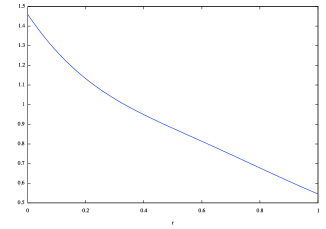
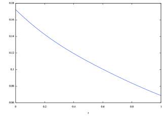
Figure 7. Plotting of $\beta_{1}(r)$ (left) and of $(\beta_{1}(r)\beta_{2}(r)-\beta_{3}(r)^{2})/r$ (right) for $r\in(0,1)$. In particular, $\beta_{1}(r)\beta_{2}(r)-\beta_{3}(r)^{2}\approx r$ for $r$ small. The plots have been drawn by Maxima v.5.28.0 (http://maxima.sourceforge.net) starting from equations $r_{2}=1$, $r_{1}=r\in(0,1)$, (4.12), (4.13), (4.14), (4.15), (4.19), (4.20), (4.21), (4.59), (4.62), (4.63), and (4.64).

As a consequence of (4.65), and up to decrease the value of $\beta_{*}$, we find

$$\beta_{1}\,r_{1}\,I_{1}^{2}+\beta_{2}\,r_{2}\,I_{2}^{2}+2\beta_{3}\,\sqrt{r_{1}r_{2}}\,I_{1}\,I_{2}\geq\beta_{*}(r_{1}\,I_{1}^{2}+r_{2}\,I_{2}^{2})\,.$$

We combine this inequality with (4.61) to prove (4.58), as claimed. Now, by (4.56) and (4.58),

$$C\,(P(\mathcal{E})-P(\mathcal{E}_{0}))\geq\sigma^{2}+r_{1}\,I_{1}^{2}+r_{2}\,I_{2}^{2}+(\varepsilon+|\sigma|)\,{\mathrm{O}}(\|u\|_{W^{1,2}}^{2})\,.$$ (4.66)

By the choice of $\varepsilon$ performed in step one, we now notice that, if for some $k=1,2$ we have

$$I_{k}^{2}\leq\frac{1}{2M(\theta_{k})}\,\int_{-\theta_{k}}^{\theta_{k}}u_{k}^{2}\,,$$

then, by Lemma 4.6,

$$\int_{-\theta_{k}}^{\theta_{k}}(u^{\prime}_{k})^{2}-u_{k}^{2}\geq\frac{1}{4}\,\Big{(}1-\frac{\theta_{k}^{2}}{\pi^{2}}\Big{)}\,\int_{-\theta_{k}}^{\theta_{k}}(u_{k}^{\prime})^{2}+\frac{1}{2}\,\Big{(}\frac{\pi^{2}}{\theta_{k}^{2}}-1\Big{)}\,\int_{-\theta_{k}}^{\theta_{k}}\,u_{k}^{2}\,.$$ (4.67)

Therefore, for $k=1,2$, either (4.67) holds true, or

$$I_{k}^{2}\geq\frac{1}{2M(\theta_{k})}\,\int_{-\theta_{k}}^{\theta_{k}}u_{k}^{2}\,.$$ (4.68)

Concerning $u_{0}$, let us notice that, by the sharp Poincaré inequality (4.40), and since $\theta_{0}<\pi/3$,

$$\int_{-\theta_{0}}^{\theta_{0}}(u^{\prime}_{0})^{2}\geq\Big{(}\frac{\pi}{2\theta_{0}}\Big{)}^{2}\int_{-\theta_{0}}^{\theta_{0}}u_{0}^{2}\geq\frac{9}{4}\,\int_{-\theta_{0}}^{\theta_{0}}u_{0}^{2}\,,$$

which gives

$$\int_{-\theta_{0}}^{\theta_{0}}(u^{\prime}_{0})^{2}-u_{0}^{2}\geq\frac{1}{3}\int_{-\theta_{0}}^{\theta_{0}}(u^{\prime}_{0})^{2}+\Big{(}\frac{3}{2}-1\Big{)}\int_{-\theta_{0}}^{\theta_{0}}u_{0}^{2}\,.$$ (4.69)

We are now going to use (4.67), (4.68), and (4.69) together with (4.66) to prove that, for some constant $C$ depending on $\mathcal{E}_{0}$, we always have

$$C\,(P(\mathcal{E})-P(\mathcal{E}_{0}))\geq\sigma^{2}+\sum_{k=0}^{2}r_{k}\int_{-\theta_{k}}^{\theta_{k}}(u_{k}^{\prime})^{2}+u_{k}^{2}\,.$$ (4.70)

We divide the argument in three cases:

Case one: We assume that (4.67) holds true for $k=1,2$. By this assumption, (4.57), and (4.69),

$$C\,(P(\mathcal{E})-P(\mathcal{E}_{0}))\geq\sigma^{2}+\sum_{k=0}^{2}r_{k}\int_{-\theta_{k}}^{\theta_{k}}(u^{\prime}_{k})^{2}+u_{k}^{2}+(\varepsilon+|\sigma|)\,{\mathrm{O}}(\|u\|_{W^{1,2}}^{2})\,,$$ (4.71)

from which (4.70) is easily proved.

Case two: We assume that (4.68) holds true for $k=1,2$. In this case, by (4.57) we obtain

$$2\,\frac{P(\mathcal{E})-P(\mathcal{E}_{0})}{1+\sigma} \geq \tau\,\Big{(}\sum_{k=0}^{2}r_{k}\int_{-\theta_{k}}^{\theta_{k}}(u^{\prime}_{k})^{2}-u_{k}^{2}\Big{)}+(1-\tau)\,2\,\frac{P(\mathcal{E})-P(\mathcal{E}_{0})}{1+\sigma}$$

$$+(\varepsilon+|\sigma|)\,{\mathrm{O}}(\|u\|_{W^{1,2}}^{2})$$

(by (4.69)) $$\geq \tau\Big{(}\frac{r_{0}}{3}\int_{-\theta_{0}}^{\theta_{0}}(u^{\prime}_{0})^{2}+\frac{r_{0}}{2}\int_{-\theta_{0}}^{\theta_{0}}u_{0}^{2}\Big{)}+\tau\,\sum_{k=1}^{2}r_{k}\int_{-\theta_{k}}^{\theta_{k}}(u^{\prime}_{k})^{2}-u_{k}^{2}$$

(by (4.66)) $$+\frac{1-\tau}{C}\,\Big{(}\sigma^{2}+r_{1}\,I_{1}^{2}+r_{2}\,I_{2}^{2}\Big{)}+(\varepsilon+|\sigma|)\,{\mathrm{O}}(\|u\|_{W^{1,2}}^{2})$$

$$\geq \tau\Big{(}\frac{r_{0}}{3}\int_{-\theta_{0}}^{\theta_{0}}(u^{\prime}_{0})^{2}+\frac{r_{0}}{2}\int_{-\theta_{0}}^{\theta_{0}}u_{0}^{2}\Big{)}+\tau\,\sum_{k=1}^{2}r_{k}\int_{-\theta_{k}}^{\theta_{k}}(u^{\prime}_{k})^{2}-u_{k}^{2}$$

(by (4.68) for $$k=1,2 +\frac{1-\tau}{C}\,\Big{(}\sigma^{2}+\sum_{k=1}^{2}\frac{r_{k}}{2M(\theta_{k})}\,\int_{-\theta_{k}}^{\theta_{k}}u_{k}^{2}\Big{)}+(\varepsilon+|\sigma|)\,{\mathrm{O}}(\|u\|_{W^{1,2}}^{2})$$)

$$\geq \tau\Big{(}\frac{r_{0}}{3}\int_{-\theta_{0}}^{\theta_{0}}(u^{\prime}_{0})^{2}+\frac{r_{0}}{2}\int_{-\theta_{0}}^{\theta_{0}}u_{0}^{2}\Big{)}+\tau\,\sum_{k=1}^{2}r_{k}\int_{-\theta_{k}}^{\theta_{k}}(u^{\prime}_{k})^{2}$$

$$+\frac{1-\tau}{2C}\,\Big{(}\sigma^{2}+\sum_{k=1}^{2}\frac{r_{k}}{2M(\theta_{k})}\,\int_{-\theta_{k}}^{\theta_{k}}u_{k}^{2}\Big{)}+(\varepsilon+|\sigma|)\,{\mathrm{O}}(\|u\|_{W^{1,2}}^{2})\,,$$

where in the last inequality we have absorbed the negative terms in $u_{k}^{2}$, $k=1,2$, by choosing $\tau$ so small to have

$$\tau\leq\frac{1-\tau}{4\,C}\min_{k=1,2}\,\frac{1}{M(\theta_{k})}\,.$$

We have thus proved (4.71), and thus (4.70), up to suitably choose $\varepsilon$ and $C$.

Case three: We assume that (4.67) holds true for $k=1$, while (4.68) holds true for $k=2$. By arguing as in case two we find, for any $\tau\in(0,1)$,

$$2\,\frac{P(\mathcal{E})-P(\mathcal{E}_{0})}{1+\sigma} \geq \tau\Big{(}\frac{r_{0}}{3}\int_{-\theta_{0}}^{\theta_{0}}(u^{\prime}_{0})^{2}+\frac{r_{0}}{2}\int_{-\theta_{0}}^{\theta_{0}}u_{0}^{2}\Big{)}+\tau\,\sum_{k=1}^{2}r_{k}\int_{-\theta_{k}}^{\theta_{k}}(u^{\prime}_{k})^{2}-u_{k}^{2}$$

$$+\frac{1-\tau}{C}\,\Big{(}\sigma^{2}+r_{1}\,I_{1}^{2}+r_{2}\,I_{2}^{2}\Big{)}+(\varepsilon+|\sigma|)\,{\mathrm{O}}(\|u\|_{W^{1,2}}^{2})\,.$$

By using (4.67) for $k=1$ and (4.68) for $k=2$, and discarding some positive terms, we find

$$2\,\frac{P(\mathcal{E})-P(\mathcal{E}_{0})}{1+\sigma} \geq \tau\,c\,\bigg{(}r_{0}\,\int_{-\theta_{0}}^{\theta_{0}}\Big{(}(u^{\prime}_{0})^{2}+u_{0}^{2}\Big{)}+r_{1}\,\int_{-\theta_{1}}^{\theta_{1}}\Big{(}(u^{\prime}_{1})^{2}+u_{1}^{2}\Big{)}+r_{2}\,\int_{-\theta_{2}}^{\theta_{2}}(u^{\prime}_{2})^{2}\bigg{)}$$

$$+\frac{1-\tau}{C}\,\Big{(}\sigma^{2}+\frac{r_{2}}{2M(\theta_{2})}\,\int_{-\theta_{2}}^{\theta_{2}}u_{2}^{2}\Big{)}-\tau\,r_{2}\int_{-\theta_{2}}^{\theta_{2}}u_{2}^{2}+(\varepsilon+|\sigma|)\,{\mathrm{O}}(\|u\|_{W^{1,2}}^{2})\,,$$

for some positive constant $c$ depending on $\mathcal{E}_{0}$. As in case two, we may choose $\tau$ small enough to have the negative term in $u_{2}^{2}$ absorbed by its positive counterpart, and come to prove (4.71). Finally, when (4.67) holds true for $k=2$ and (4.68) holds true for $k=1$ (note that, formally, this is a fourth different case, as $m_{2}>m_{1}$), then we just repeat the very same argument. Summarizing, we have proved the validity of (4.70), which of course implies (4.49). The theorem is proved in the case $m_{2}>m_{1}$.

Step three: We now address the case $m_{2}=m_{1}$. In this case we set $r=r_{1}=r_{2}$, $m=m_{1}=m_{2}$, and $\theta=\theta_{1}=\theta_{2}=2\pi/3$. Once again, up to scaling, we may assume that $r=1$, so that

$$m=\frac{2\pi}{3}+\frac{\sqrt{3}}{4}\,,\qquad P(\mathcal{E}_{0})=4\,m=\frac{8\,\pi}{3}+\sqrt{3}\,.$$

The volume constraints now take the form

$$\Big{(}(1+\sigma)^{-2}-1\Big{)}\,m=I_{1}+\int_{-\sqrt{3}/2}^{\sqrt{3}/2}v_{0}=I_{2}-\int_{-\sqrt{3}/2}^{\sqrt{3}/2}v_{0}\,,$$

so that, by arguing as in step one, we find, in analogy to (4.54) and (4.55),

$$\int_{-\sqrt{3}/2}^{\sqrt{3}/2}v_{0}=\frac{I_{2}-I_{1}}{2}\,,\qquad\sigma^{2}+{\mathrm{O}}(|\sigma|^{3})=\frac{(I_{1}+I_{2})^{2}}{4\,m^{2}}\,.$$ (4.72)

By Lemma 4.5 we have (4.60) for $k=1,2$, and, similarly,

$$\int_{-\sqrt{3}/2}^{\sqrt{3}/2}(v_{0}^{\prime})^{2}\geq\int_{-\sqrt{3}/2}^{\sqrt{3}/2}v_{0}^{2}+g\Big{(}\frac{\sqrt{3}}{2}\Big{)}\,\Big{(}\int_{-\sqrt{3}/2}^{\sqrt{3}/2}v_{0}\Big{)}^{2}=\int_{-\sqrt{3}/2}^{\sqrt{3}/2}v_{0}^{2}+g\Big{(}\frac{\sqrt{3}}{2}\Big{)}\,\frac{(I_{2}-I_{1})^{2}}{4}\,.$$ (4.73)

(Notice that $\sqrt{3}/2<\pi/2$, thus $g(\sqrt{3}/2)$ is positive.) By (4.72) and (4.73), and since $|\sigma|={\mathrm{O}}(\|u\|_{L^{2}}^{2})$, from (4.29) we deduce

$$2\,\frac{P(\mathcal{E})-P(\mathcal{E}_{0})}{1+\sigma} = \int_{-\,\sqrt{3}/2}^{\,\sqrt{3}/2}(v^{\prime}_{0})^{2}+\sum_{k=1}^{2}\,\int_{-2\pi/3}^{2\pi/3}(u^{\prime}_{k})^{2}-u_{k}^{2}+\frac{\sigma^{2}}{2}\,P(\mathcal{E}_{0})+(\varepsilon+|\sigma|)\,{\mathrm{O}}(\|u\|_{W^{1,2}}^{2})$$

$$\geq \int_{-\sqrt{3}/2}^{\sqrt{3}/2}v_{0}^{2}+g\Big{(}\frac{\sqrt{3}}{2}\Big{)}\,\frac{(I_{2}-I_{1})^{2}}{4}+g\Big{(}\frac{2\pi}{3}\Big{)}(I_{1}^{2}+I_{2}^{2})+\frac{(I_{1}+I_{2})^{2}}{2\,m}$$

$$+(\varepsilon+|\sigma|)\,{\mathrm{O}}(\|u\|_{W^{1,2}}^{2})$$

$$\geq \int_{-\sqrt{3}/2}^{\sqrt{3}/2}v_{0}^{2}+\alpha_{1}\,I_{1}^{2}+\alpha_{2}\,I_{2}^{2}+2\alpha_{3}\,I_{1}\,I_{2}\,,+(\varepsilon+|\sigma|)\,{\mathrm{O}}(\|u\|_{W^{1,2}}^{2})\,,$$

provided we set

$$\alpha_{1}=\alpha_{2}=\frac{1}{4}\,g\Big{(}\frac{\sqrt{3}}{2}\Big{)}+g\Big{(}\frac{2\pi}{3}\Big{)}+\frac{1}{2m}$$

$$\alpha_{3}=-\frac{1}{4}\,g\Big{(}\frac{\sqrt{3}}{2}\Big{)}+\frac{1}{2m}\,.$$

By direct evaluation we see that $\alpha_{1}>0$ and $\alpha_{1}\alpha_{2}-\alpha_{3}^{2}>0$. Therefore there exists $\alpha_{*}>0$ such that $\alpha_{1}\,I_{1}^{2}+\alpha_{2}\,I_{2}^{2}+2\alpha_{3}\,I_{1}\,I_{2}\geq\alpha_{*}(I_{1}^{2}+I_{2}^{2})$, and thus

$$2\,\frac{P(\mathcal{E})-P(\mathcal{E}_{0})}{1+\sigma}\geq\int_{-\sqrt{3}/2}^{\sqrt{3}/2}v_{0}^{2}+\alpha_{*}\,(I_{1}^{2}+I_{2}^{2})+(\varepsilon+|\sigma|)\,{\mathrm{O}}(\|u\|_{W^{1,2}}^{2})\,.$$ (4.74)

We conclude the proof exactly as in step two, with (4.74) playing the role of (4.58), and with

$$\int_{-\sqrt{3}/2}^{\sqrt{3}/2}(v^{\prime}_{0})^{2}\geq\frac{1}{2}\int_{-\sqrt{3}/2}^{\sqrt{3}/2}(v^{\prime}_{0})^{2}+v_{0}^{2}$$ (4.75)

playing the role of (4.69). (Note that (4.75) follows trivially from (4.73).) This completes the proof of Theorem 4.7. ∎

Appendix A The qualitative stability theorem and a selection principle

Here we prove a qualitative stability theorem (Theorem A.1) and a selection principle for quantitative stability inequalities (Theorem A.2) on isoperimetric $N$-clusters in $\mathbb{R}^{n}$ with $n$ and $N$ arbitrary. These results are not entirely standard because of some compactness issues that need to be handled under a multiple volumes constraint. Such compactness issues are usually simpler to address in dimension $n=2$ (because perimeter controls diameter on indecomposable sets of finite perimeter), and in this paper we only need the above results in the case $N=n=2$. However, Theorem A.1 is interesting in itself and it is useful knowing its validity in the general case. Theorem A.2, although of course of more technical nature, should still reveal useful in addressing the quantitative stability problem for double-bubbles in higher dimensions. Moreover, the simplifications one has setting $n=2$ seem not that significant, at least if one exploits the arguments we know to prove these results. For these reasons we have decided to prove these theorems in full generality.

The setting considered in this appendix will be as follows. Given a $N$-cluster $\mathcal{E}_{0}$ in $\mathbb{R}^{n}$ one says that $\mathcal{E}_{0}$ is an isoperimetric cluster if $P(\mathcal{E}_{0})\leq P(\mathcal{E})$ whenever $\mathrm{vol}\,(\mathcal{E})=\mathrm{vol}\,(\mathcal{E}_{0})$, and that $\mathcal{E}_{0}$ is uniquely minimizing if $P(\mathcal{E})=P(\mathcal{E}_{0})$ and $\mathrm{vol}\,(\mathcal{E})=\mathrm{vol}\,(\mathcal{E}_{0})$ imply the existence of an isometry $f:\mathbb{R}^{n}\to\mathbb{R}^{n}$ such that $f(\mathcal{E})=\mathcal{E}_{0}$, where we have set $f(\mathcal{E})(h)=f(\mathcal{E}(h))$ for every $h=1,...,N$. For a uniquely minimizing isoperimetric cluster $\mathcal{E}_{0}$ in $\mathbb{R}^{n}$, we set

$$\mathcal{M}_{0} = \big{\{}\mathcal{E}:\ \mathcal{E}\text{ is an $N$-cluster, }\mathrm{vol}\,(\mathcal{E})=\mathrm{vol}\,(\mathcal{E}_{0})\big{\}}\,,$$

$$\delta(\mathcal{E}) = P(\mathcal{E})-P(\mathcal{E}_{0})\,,$$

$$\alpha(\mathcal{E}) = \inf\big{\{}\mathrm{d}(\mathcal{E},f(\mathcal{E}_{0})):\mbox{$f:\mathbb{R}^{n}\to\mathbb{R}^{n}$ is an isometry}\big{\}}\,,$$

where $\mathrm{d}(\mathcal{E},\mathcal{F})=(1/2)\,\sum_{h=0}^{N}|\mathcal{E}(h)\Delta\mathcal{F}(h)|$. Note that if $\mathcal{E}\in\mathcal{M}_{0}$, then $\delta(\mathcal{E})$ and $\alpha(\mathcal{E})$ are both positive unless $\mathcal{E}$ is isometric to $\mathcal{E}_{0}$. In analogy with the case $N=1$ [FMP08], one may ask about the validity of a quantitative stability inequality of the form

$$\delta(\mathcal{E})\geq\kappa\,\alpha(\mathcal{E})^{2}\,,\qquad\forall\mathcal{E}\in\mathcal{M}_{0}\,,$$ (A.1)

for some $\kappa>0$. As a first step in this direction, one wants to prove the following theorem.

Theorem A.1.

If $\mathcal{E}_{0}$ is a uniquely minimizing isoperimetric cluster in $\mathbb{R}^{n}$, $n\geq 2$, then for every $\eta>0$ there exists $\delta>0$ such that if $\mathrm{vol}\,(\mathcal{E})=\mathrm{vol}\,(\mathcal{E}_{0})$ and $P(\mathcal{E})\leq P(\mathcal{E}_{0})+\delta$, then $\alpha(\mathcal{E})\leq\eta$.

Once Theorem A.1 is proved, and following the approach proposed in [CL12] to address (A.1) in the case $N=1$, one notices that by a simple contradiction argument (A.1) is equivalent to showing that $\kappa(\mathcal{E}_{0})>0$, where we have set

$$\kappa(\mathcal{E}_{0})=\inf\big{\{}\liminf_{k\to\infty}\frac{\delta(\mathcal{E}_{k})}{\alpha(\mathcal{E}_{k})^{2}}:\{\mathcal{E}_{k}\}_{k\in\mathbb{N}}\subset\mathcal{M}_{0}\,,\alpha(\mathcal{E}_{k})>0\,,\mathcal{E}_{k}\to\mathcal{E}_{0}\big{\}}\,.$$ (A.2)

By applying a selection principle to minimizing sequences in (A.2), one ends up reducing the proof of (A.1) to the case when $\mathcal{E}$ is a $(\Lambda,r_{0})$-minimizing cluster in $\mathbb{R}^{n}$ for some $\Lambda\geq 0$ and $r_{0}>0$ depending on $\mathcal{E}_{0}$ only. In the case $N=1$, as shown in [CL12], this reduction allows one to complete the proof of (A.1) quite easily thanks to a decomposition in spherical harmonics originally introduced by Fuglede [Fug89]. At the same time, as shown in this paper, this strategy works to prove (A.1) when $N=n=2$. It thus seems interesting to know that one can always attack (A.1) from this angle. More precisely, we have the following result.

Theorem A.2.

If $\mathcal{E}_{0}$ is a uniquely minimizing isoperimetric cluster in $\mathbb{R}^{n}$ with $\kappa(\mathcal{E}_{0})<\infty$, then there exist positive constants $\Lambda$, $r_{0}$, and $R_{0}$ and a sequence of $(\Lambda,r_{0})$-minimizing clusters $\{\mathcal{E}_{k}\}_{k\in\mathbb{N}}\subset\mathcal{M}_{0}$ with

$$\inf_{k\in\mathbb{N}}\alpha(\mathcal{E}_{k})>0\,,\qquad\lim_{k\to\infty}\mathrm{d}(\mathcal{E}_{k},\mathcal{E}_{0})=0\,,\qquad\lim_{k\to\infty}\frac{\delta(\mathcal{E}_{k})}{\alpha(\mathcal{E}_{k})^{2}}=\kappa(\mathcal{E}_{0})\,.$$

Moreover, $\mathcal{E}_{k}(h)\subset B_{R_{0}}$ for every $h=1,...,N$, and each $\mathcal{E}_{k}$ satisfies the global, volume-constrained minimality property

$$P(\mathcal{E}_{k})\leq P(\mathcal{F})+3\,\sqrt{\alpha(\mathcal{E}_{k})}\,\mathrm{d}(\mathcal{F},\mathcal{E}_{k})\,,\qquad\forall\mathcal{F}\in\mathcal{M}_{0}\,.$$ (A.3)

Remark A.1.

The assumption $\kappa(\mathcal{E}_{0})<\infty$ is essentially equivalent to showing the existence of a one-parameter family of clusters $\{\mathcal{E}_{t}\}_{|t|<\varepsilon}$ with $\mathrm{vol}\,(\mathcal{E}_{t})=\mathrm{vol}\,(\mathcal{E}_{0})$, $\alpha(\mathcal{E}_{t})>0$, $P(\mathcal{E}_{t})-P(\mathcal{E}_{0})\leq C\,t^{2}$, and $\alpha(\mathcal{E}_{t})\geq|t|/C$ for every $|t|<\varepsilon$. By Theorem A.3 below, it is not difficult to define $\mathcal{E}_{t}$ satisfying the first three conditions: what is not immediate, however, is proving that $\alpha(\mathcal{E}_{t})\geq|t|/C$. When $N=1$ or $N=2$ (see section 2.2 for the latter case) one can easily address this point by exploiting the symmetries of the corresponding isoperimetric clusters (balls or standard double-bubbles). For general $N$ one does not expect to have symmetry properties or to explicitly characterize isoperimetric clusters. Nevertheless, it is always true that $\kappa(\mathcal{E}_{0})<\infty$. We shall not further discuss this issue here.

We now turn to prove Theorem A.1 and Theorem A.2. As explained the issue is the lack of global compactness, and thus of the possible loss of volume at infinity. This can be fixed by exploiting an argument similar to the one used in Almgren’s proof [Alm76] of the existence of isoperimetric clusters for every given volume vector, see also [Mag12, Chapter 29]. Almgren’s argument uses truncations and translations of pieces of the quasi-isoperimetric clusters, so what one needs to do is taking track of what happens to $\alpha(\mathcal{E})$ under these operations. The following theorem is a key tool in implementing this strategy. It is a variant of [Alm76, Proposition VI.12], see also [Mag12, Corollary 29.17]. The necessary modifications with respect to [Mag12, Corollary 29.17] are described in [CLM14, Appendix B], so that we omit to give a detailed proof in here.

Theorem A.3 (Volume-fixing variations).

If $\mathcal{E}_{0}$ is a $N$-cluster in $\mathbb{R}^{n}$, then there exist positive constants $r_{0}$, $\varepsilon_{0}$, $R_{0}$ and $C_{0}$ (depending on $\mathcal{E}_{0}$) with the following property. Let $\mathcal{E}$ be a $N$-cluster in $\mathbb{R}^{n}$ with

$$\mathrm{d}(\mathcal{E},\mathcal{E}_{0})\leq\varepsilon_{0}\,,$$ (A.4)

and let $\mathcal{F}$ be a $N$-clusters in $\mathbb{R}^{n}$ such that either

$$\bigcup_{h=1}^{N}\mathcal{F}(h)\Delta\mathcal{E}(h)\subset\subset B_{x,r_{0}}\,,\qquad\mbox{for some $x\in\mathbb{R}^{n}$}\,,$$ (A.5)

or

$$\mathrm{d}(\mathcal{E},\mathcal{F})\leq\omega_{n}\,r_{0}^{n}\,,\qquad\bigcup_{h=1}^{N}\mathcal{F}(h)\Delta\mathcal{E}(h)\subset\mathbb{R}^{n}\setminus B_{R}\,,\qquad\begin{split}&\mbox{if there exists $R>0$ s.t.}\\ &\bigcup_{h=1}^{N}\mathcal{E}_{0}(h)\subset\subset B_{R}\,.\end{split}$$ (A.6)

Then there exists a $N$-cluster $\mathcal{F}^{\prime}$ such that

$$\bigcup_{h=1}^{N}\mathcal{F}^{\prime}(h)\Delta\mathcal{F}(h) \subset\subset \left\{\begin{split}&B_{R_{0}}\setminus\overline{B_{x,r_{0}}}\,,&\qquad\mbox{if \eqref{volumefix hp 1} holds}\,,\\ &B_{R}\,,&\qquad\mbox{if \eqref{volumefix hp 1x} holds}\,,\end{split}\right.$$ (A.7)

$$\mathrm{vol}\,(\mathcal{F}^{\prime}) = \mathrm{vol}\,(\mathcal{E})\,,$$ (A.8)

$$|P(\mathcal{F}^{\prime})-P(\mathcal{F})| \leq C_{0}\,P(\mathcal{E})\,|\mathrm{vol}\,(\mathcal{F})-\mathrm{vol}\,(\mathcal{E})|\,,$$ (A.9)

$$|\mathrm{d}(\mathcal{F}^{\prime},\mathcal{E})-\mathrm{d}(\mathcal{F},\mathcal{E})| \leq C_{0}\,P(\mathcal{E})\,|\mathrm{vol}\,(\mathcal{F})-\mathrm{vol}\,(\mathcal{E})|\,,$$ (A.10)

$$\sum_{h=0}^{N}\int_{\mathcal{F}^{\prime}(h)\Delta\mathcal{F}(h)}J \leq C_{0}\,\|J\|_{L^{\infty}(B_{R_{0}})}\,P(\mathcal{E})\,\,|\mathrm{vol}\,(\mathcal{F})-\mathrm{vol}\,(\mathcal{E})|\,,$$ (A.11)

for every Borel function $J:\mathbb{R}^{n}\to[0,\infty)$ which is locally bounded.

We now prove Theorem A.1 and Theorem A.2 for a fixed uniquely minimizing isoperimetric cluster $\mathcal{E}_{0}$. Thanks to [Mag12, Theorem 29.1], there exists $R>0$ such that $\mathcal{E}_{0}(h)\subset\subset B_{R}$ for every $h=1,...,N$. Moreover we shall use the obvious inequality

$$|\alpha(\mathcal{E})-\alpha(\mathcal{F})|\leq\mathrm{d}(\mathcal{E},\mathcal{F})\,,\qquad\mbox{for every $N$-clusters $\mathcal{E}$ and $\mathcal{F}$}\,.$$ (A.12)

Proof of Theorem A.1.

The argument has several points in common with [Mag12, Proof of Theorem 29.1]. Arguing by contradiction, we assume the existence of $\eta_{*}>0$ and of a sequence $\{\mathcal{E}_{k}\}_{k\in\mathbb{N}}$ of $N$-clusters such that $\mathrm{vol}\,(\mathcal{E}_{k})=\mathrm{vol}\,(\mathcal{E}_{0})$ for every $k\in\mathbb{N}$ and

$$\lim_{k\to\infty}P(\mathcal{E}_{k})=P(\mathcal{E}_{0})\,,\qquad\lim_{k\to\infty}\alpha(\mathcal{E}_{k})=\eta_{*}\,.$$

By arguing as in step one of the proof of [Mag12, Theorem 29.1] we identify for each cluster $\mathcal{E}_{k}$ a suitable region (constructed as a union of balls of radius $S$, see the right-hand side of (A.13)) inside of which, in the spirit of Theorem A.3, we can perform volume-fixing variations of $\mathcal{E}_{k}$ with uniform bounds in $k$. More precisely, there exist positive constants $\varepsilon_{1}$, $C_{1}$, and $S$, points $\{x_{k}(h)\}_{k\in\mathbb{N}}\subset\mathbb{R}^{n}$ ($1\leq h\leq N$), and $C^{1}$-maps $\Phi_{k}:((-\varepsilon_{1},\varepsilon_{1})^{N+1}\cap V)\times\mathbb{R}^{n}\to\mathbb{R}^{n}$, (here $V=\{\mathbf{a}\in\mathbb{R}^{N+1}:\sum_{h=0}^{N}\mathbf{a}(h)=0\}$) with the property that (up to extracting subsequences in $k$) $\Phi_{k}(\mathbf{a},\cdot)$ is a $C^{1}$-diffeomorphism on $\mathbb{R}^{n}$ for every $\mathbf{a}\in(-\varepsilon_{1},\varepsilon_{1})^{N+1}\cap V$, and, moreover, for every $\mathbf{a}\in(-\varepsilon_{1},\varepsilon_{1})^{N+1}\cap V$ and for every $\mathcal{H}^{n-1}$-rectifiable set $\Sigma\subset\mathbb{R}^{n}$, it holds

$$\big{\{}x\in\mathbb{R}^{n}:\Phi_{k}(\mathbf{a},x)\neq x\big{\}} \subset\subset \bigcup_{h=1}^{N}B(x_{k}(h),S)\,,$$ (A.13)

$$\big{|}\Phi_{k}(\mathbf{a},\mathcal{E}_{k}(h))\big{|} = |\mathcal{E}_{k}(h)|+\mathbf{a}(h)\,,$$ (A.14)

$$\big{|}\mathcal{H}^{n-1}\big{(}\Phi_{k}(\mathbf{a},\Sigma)\big{)}-\mathcal{H}^{n-1}(\Sigma)\big{|} \leq C_{1}\,\mathcal{H}^{n-1}(\Sigma)\,|\mathbf{a}|\,,$$ (A.15)

$$\big{|}\Phi_{k}(\mathbf{a},\mathcal{E}_{k}(h))\Delta\mathcal{E}_{k}(h)\big{|} \leq C_{1}\,P(\mathcal{E}_{k}(h))\,|\mathbf{a}|\,.$$ (A.16)

Note that (A.16) is not mentioned in step one of the proof of [Mag12, Theorem 29.1], but that it can be easily achieved by exploiting [CLM14, Lemma B.2]. At the same time, by arguing as in step two of the proof of [Mag12, Theorem 29.1], we see that there exist positive constants $\varepsilon_{0}$ and $L$ (depending on $\{\mathcal{E}_{k}\}_{k\in\mathbb{N}}$ only) such that for every $\eta<\varepsilon_{0}$, $k\in\mathbb{N}$, and $h=1,\dots,N$, we can find finitely many points $\{y_{k}(h,i)\}_{i=1}^{L_{k}(h)}\subset\mathbb{R}^{n}$ such that

$$\Big{|}\mathcal{E}_{k}(h)\setminus\bigcup_{i=1}^{L_{k}(h)}B(y_{k}(h,i),2)\Big{|}<\frac{\eta}{N}\,,\qquad L_{k}(h)\leq\frac{L}{\eta^{n}}\,.$$ (A.17)

Let us now consider the closed sets

$$F_{k}=\bigcup_{h=1}^{N}\,\overline{B}(x_{k}(h),S)\cup\bigcup_{i=1}^{L_{k}(h)}\,\overline{B}(y_{k}(h,i),2)\,,\qquad k\in\mathbb{N}\,.$$

Since, by (A.17),

$$\sum_{h=1}^{N}|\mathcal{E}_{k}(h)\setminus F_{k}|\leq\eta\,,\qquad\forall k\in\mathbb{N}\,,$$ (A.18)

the truncation lemma [Mag12, Lemma 29.12] guarantees the existence of $r_{0}\in[0,7n\,\eta^{1/n}]$ such that, if $I_{\varepsilon}(X)=\{x\in\mathbb{R}^{n}:\hbox{dist}(x,X)<\varepsilon\}$ denotes the $\varepsilon$-neighborhood of $X\subset\mathbb{R}^{n}$, and if $\{\mathcal{E}^{\prime}_{k}\}_{k\in\mathbb{N}}$ are the $N$-clusters defined by $\mathcal{E}^{\prime}_{k}(h)=\mathcal{E}_{k}(h)\cap I_{r_{0}}(F_{k})$, $1\leq h\leq N$, then

$$P(\mathcal{E}^{\prime}_{k})\leq P(\mathcal{E}_{k})-\frac{\mathrm{d}(\mathcal{E}^{\prime}_{k},\mathcal{E}_{k})}{4\,\eta^{1/n}}\,.$$ (A.19)

By (A.18) we have $\mathrm{d}(\mathcal{E}^{\prime}_{k},\mathcal{E}_{k})\leq\eta$, so that by (A.12)

$$\alpha(\mathcal{E}_{k}^{\prime})\geq\alpha(\mathcal{E}_{k})-\eta\,,\qquad\forall k\in\mathbb{N}\,.$$ (A.20)

If we set $\mathbf{a}_{k}(h)=|\mathcal{E}_{k}(h)|-|\mathcal{E}^{\prime}_{k}(h)|=|\mathcal{E}_{k}(h)\setminus I_{r_{0}}(F_{k})|$ for $1\leq h\leq N$ and $\mathbf{a}_{k}(0)=-\sum_{h=1}^{N}\mathbf{a}_{k}(h)$, and if we require $\eta\leq\varepsilon_{1}$, then $\mathbf{a}_{k}\in(-\varepsilon_{1},\varepsilon_{1})^{N+1}\cap V$ for every $k\in\mathbb{N}$. We may thus define a sequence of clusters $\{\mathcal{E}_{k}^{\prime\prime}\}_{k\in\mathbb{N}}$ by setting

$$\mathcal{E}_{k}^{\prime\prime}(h)=\Phi_{k}(\mathbf{a}_{k},\mathcal{E}_{k}^{\prime}(h))\,,\qquad 1\leq h\leq N\,.$$

Let us notice that, by (A.13), $\Phi_{k}(x)=x$ in an open neighborhood of $\mathbb{R}^{n}\setminus F_{k}$, so that, in fact, $\Phi_{k}(\mathbf{a}_{k},\mathcal{E}_{k}^{\prime}(h))=\Phi_{k}(\mathbf{a}_{k},\mathcal{E}_{k}(h))\cap I_{r_{0}}(F_{k})$. Therefore, by (A.14), (A.15), (A.19), and the definition of the $\mathbf{a}_{k}$’s, much as in step two of the proof of [Mag12, Theorem 29.1], we obtain that

$$\mathrm{vol}\,(\mathcal{E}_{k}^{\prime\prime}) = \mathrm{vol}\,(\mathcal{E}_{k})=\mathrm{vol}\,(\mathcal{E}_{0})\,,$$ (A.21)

$$P(\mathcal{E}_{k}^{\prime\prime}) \leq P(\mathcal{E}_{k})+\Big{(}4C_{1}P(\mathcal{E}_{0})-\frac{1}{4\eta^{1/n}}\Big{)}\,\mathrm{d}(\mathcal{E}^{\prime}_{k},\mathcal{E}_{k})\,;$$ (A.22)

moreover, this time taking into account (A.16), and since $\mathrm{d}(\mathcal{E}_{k},\mathcal{E}_{k}^{\prime})\leq\eta$, we find that

$$\mathrm{d}(\mathcal{E}_{k}^{\prime\prime},\mathcal{E}_{k})\leq\eta+C_{1}\,P(\mathcal{E}_{k})\,|\mathbf{a}_{k}|\leq C_{2}\,\eta\,,$$ (A.23)

where $C_{2}$ is a constant depending on $\{\mathcal{E}_{k}\}_{k\in\mathbb{N}}$ only; in particular, by (A.23) and (A.12)

$$\alpha(\mathcal{E}_{k}^{\prime\prime})\geq\alpha(\mathcal{E}_{k})-C_{2}\eta\geq\frac{\eta_{*}}{2}\,,$$ (A.24)

provided $\eta$ is small enough; similarly, up to further decreasing the value of $\eta$, (A.22) gives us

$$P(\mathcal{E}_{k}^{\prime\prime})\leq P(\mathcal{E}_{k})\,,\qquad\forall k\in\mathbb{N}\,.$$ (A.25)

Summarizing, by taking into account (A.21), (A.25), and (A.24) we see that $\{\mathcal{E}_{k}^{\prime\prime}\}_{k\in\mathbb{N}}$ satisfies

$$\lim_{k\to\infty}P(\mathcal{E}_{k}^{\prime\prime})=P(\mathcal{E}_{0})\,,\qquad\liminf_{k\to\infty}\alpha(\mathcal{E}_{k}^{\prime\prime})\geq\frac{\eta_{*}}{2}\,;$$ (A.26)

moreover, by the definition of $\mathcal{E}_{k}^{\prime}$ and $\mathcal{E}_{k}^{\prime\prime}$, and thanks to (A.13), for every $k\in\mathbb{N}$ we find

$$\bigcup_{h=1}^{N}\mathcal{E}^{\prime\prime}_{k}(h)\subset\subset G_{k}=\overline{I_{2\,r_{0}}(F_{k})}\,,$$

where $G_{k}$ is a closed set with at most $L_{0}=L_{0}(n,N,L,\eta)$ connected components of diameter at most $S_{0}=S_{0}(S,r_{0},L_{0})$ with $r_{0}\leq 7n\eta^{1/n}$. Clearly, the mutual distances between these connected components may tend to infinity or not: in any case we can find $\{z_{k}^{j}\}_{j=1}^{M}\subset\mathbb{R}^{n}$, $1\leq M\leq L_{0}$, such that for every $k\in\mathbb{N}$ and $1\leq j_{1}<j_{2}\leq M$ (if $M\geq 2$)

$$\bigcup_{h=1}^{N}\mathcal{E}^{\prime\prime}_{k}(h)\subset\subset\bigcup_{j=1}^{M}B(z_{k}^{j},S_{0})\,,\qquad\lim_{k\to\infty}|z_{k}^{j_{1}}-z_{k}^{j_{2}}|=\infty\,.$$

In particular, $\{B(z_{k}^{j},S_{0})\}_{j=1}^{M}$ is a disjoint family of balls if $M\geq 2$ and $k$ is large enough. Let us assume, as we may up to isometries, that $\alpha(\mathcal{E}_{k}^{\prime\prime})=\mathrm{d}(\mathcal{E}_{k}^{\prime\prime},\mathcal{E}_{0})$. Up to relabeling the index $j$ and up to take $k$ large enough, by taking into account $\mathcal{E}_{0}(h)\subset\subset B_{R}$ for every $h=1,..,N$, we may ensure that

$$\alpha(\mathcal{E}_{k}^{\prime\prime})=\sum_{h=1}^{N}\Big{|}\Big{(}\mathcal{E}_{k}^{\prime\prime}(h)\Delta\mathcal{E}_{0}(h)\Big{)}\cap B(z_{k}^{1},S_{0})\Big{|}\,,\qquad 0=\sum_{h=1}^{N}\sum_{j=2}^{M}\Big{|}\mathcal{E}_{0}(h)\cap B(z_{k}^{j},S_{0})\Big{|}\,.$$

(This implies, in particular, that $|z_{k}^{1}|\leq R+S_{0}$.) Let us finally consider vectors $\{y_{k}^{j}\}_{j=2}^{M}$ such that the balls $\{B(z_{k}^{j}+y_{k}^{j},S_{0})\}_{j=2}^{M}$ lie at mutually positive distance at least $2\,(S_{0}+R)$ and at most $2\,(S_{0}+R)\,M$ one from each other and from $B(z_{k}^{1},S_{0})$, and define a sequence $\{\mathcal{E}_{k}^{\prime\prime\prime}\}_{k\in\mathbb{N}}$ so that, for $h=1,\dots,N$,

$$\mathcal{E}_{k}^{\prime\prime\prime}(h)\cap B(z_{k}^{1},S_{0}) = \mathcal{E}_{k}^{\prime\prime}(h)\cap B(z_{k}^{1},S_{0})\,,$$

$$\mathcal{E}_{k}^{\prime\prime\prime}(h)\cap B(z_{k}^{j}+y_{k}^{j},S_{0}) = \big{(}\mathcal{E}_{k}^{\prime\prime}(h)\cap B(z_{k}^{j},S_{0})\big{)}+y_{k}^{j}\,,\qquad 2\leq j\leq M\,,\quad$$

$$\mathcal{E}_{k}^{\prime\prime\prime}(h)\setminus\Big{(}B(z_{k}^{1},S_{0})\cup\bigcup_{j=2}^{M}B(z_{k}^{j},S_{0})\Big{)} = \emptyset\,.$$

In this way, by construction of $y_{k}^{j}$ and since $\mathcal{E}_{0}\subset\subset B_{R}$, it must be $\alpha(\mathcal{E}_{k}^{\prime\prime\prime})=\alpha(\mathcal{E}_{k}^{\prime\prime})$ for every $k$ large enough, so that $\liminf_{k\to\infty}\alpha(\mathcal{E}_{k}^{\prime\prime\prime})\geq\eta_{*}/2$. At the same time, there exists $Q$ depending on $S_{0}$, $R$, and $M$ only, such that $\mathcal{E}_{k}^{\prime\prime\prime}\subset B_{Q}$ for every $k\in\mathbb{N}$, so that by $\lim_{k\to\infty}P(\mathcal{E}_{k}^{\prime\prime\prime})=P(\mathcal{E}_{0})$, $\mathrm{vol}\,(\mathcal{E}_{k}^{\prime\prime\prime})=\mathrm{vol}\,(\mathcal{E}_{0})$, and by the standard compactness theorem [Mag12, Proposition 29.5], there exists a $N$-cluster $\mathcal{E}_{*}$ such that, up to extracting subsequences, $\mathrm{d}(\mathcal{E}_{k}^{\prime\prime\prime},\mathcal{E}_{*})\to 0$ as $k\to\infty$. Therefore, it holds $\mathrm{vol}\,(\mathcal{E}_{*})=\mathrm{vol}\,(\mathcal{E}_{0})$, $P(\mathcal{E}_{*})=P(\mathcal{E}_{0})$, and $\alpha(\mathcal{E}_{*})\geq\eta_{*}/2$, a contradiction to the unique minimality of $\mathcal{E}_{0}$. ∎

Proof of Theorem A.2.

Let us consider a recovery sequence $\{\mathcal{F}_{k}\}_{k\in\mathbb{N}}\subset\mathcal{M}_{0}$ for $\kappa(\mathcal{E}_{0})$, that is

$$\inf_{k\in\mathbb{N}}\alpha(\mathcal{F}_{k})>0\,,\qquad\lim_{k\to\infty}\mathrm{d}(\mathcal{F}_{k},\mathcal{E}_{0})=0\,,\qquad\kappa(\mathcal{E}_{0})=\lim_{k\to\infty}\frac{\delta(\mathcal{F}_{k})}{\alpha(\mathcal{F}_{k})^{2}}\,,$$ (A.27)

and notice that, since $\kappa(\mathcal{E}_{0})<\infty$, we have

$$\lim_{k\to\infty}\alpha(\mathcal{F}_{k})=0\,,\qquad P(\mathcal{F}_{k})=P(\mathcal{E}_{0})+\kappa(\mathcal{E}_{0})\,\alpha(\mathcal{F}_{k})^{2}+o(\alpha(\mathcal{F}_{k})^{2})\,.$$ (A.28)

Without loss of generality, we may assume that, for all $k\in\mathbb{N}$, and for $\beta>0$ to be suitably chosen,

$$P(\mathcal{F}_{k})\leq P(\mathcal{E}_{0})+(\kappa(\mathcal{E}_{0})+1)\,\alpha(\mathcal{F}_{k})^{2}\,,\qquad\alpha(\mathcal{F}_{k})\leq\beta\,.$$ (A.29)

We claim that for every $k$ large enough there exists a minimizer $\mathcal{E}_{k}$ in the problem

$$\gamma_{k}(\mathcal{E}_{0})=\inf\big{\{}P(\mathcal{E})+|\alpha(\mathcal{E})-\alpha(\mathcal{F}_{k})|^{3/2}:\ \mathcal{E}\in\mathcal{M}_{0}\big{\}}\,,$$ (A.30)

and that

$$\alpha(\mathcal{E}_{k}) \geq \frac{\alpha(\mathcal{F}_{k})}{3}\,,$$ (A.31)

$$|\alpha(\mathcal{E}_{k})-\alpha(\mathcal{F}_{k})| \leq (\kappa(\mathcal{E}_{0})+1)^{2/3}\,\alpha(\mathcal{F}_{k})^{4/3}\,,$$ (A.32)

$$\bigcup_{h=1}^{N}\mathcal{E}_{k}(h) \subset B_{R_{0}}\,,\qquad R_{0}=R+7n\beta^{1/n}\,,$$ (A.33)

$$P(\mathcal{E}_{k}) = P(\mathcal{E}_{0})+\kappa(\mathcal{E}_{0})\,\alpha(\mathcal{E}_{k})^{2}+o(\alpha(\mathcal{E}_{k})^{2})\,,\qquad\mbox{as $k\to\infty$}\,.$$ (A.34)

Indeed, given $k\in\mathbb{N}$, let $\{\mathcal{E}_{k,j}\}_{j\in\mathbb{N}}$ be a minimizing sequence in (A.30). Since $\mathcal{F}_{k}$ is admissible in (A.30) and by (A.29), provided $\beta$ is small enough, we may assume without loss of generality that

$$\left\{\begin{split}&P(\mathcal{E}_{k,j})+|\alpha(\mathcal{E}_{k,j})-\alpha(\mathcal{F}_{k})|^{3/2}\leq P(\mathcal{F}_{k})\\ &P(\mathcal{E}_{k,j})\leq P(\mathcal{E}_{0})+1\end{split}\right.\,,\qquad\forall k\,,j\in\mathbb{N}\,.$$ (A.35)

By subtracting $P(\mathcal{E}_{0})$ in this last inequality, by $P(\mathcal{E}_{k,j})\geq P(\mathcal{E}_{0})$, and by (A.29) we thus get

$$|\alpha(\mathcal{E}_{k,j})-\alpha(\mathcal{F}_{k})|^{3/2}\leq(\kappa(\mathcal{E}_{0})+1)\,\alpha(\mathcal{F}_{k})^{2}\,,\qquad\forall k\,,j\in\mathbb{N}\,.$$ (A.36)

In particular, provided $\beta$ is small enough, we find

$$\frac{\alpha(\mathcal{F}_{k})}{2}\leq\alpha(\mathcal{E}_{k,j})\leq\frac{3}{2}\,\alpha(\mathcal{F}_{k})\,,\qquad\forall k\,,j\in\mathbb{N}\,.$$ (A.37)

We now construct new minimizing sequences $\{\widetilde{\mathcal{E}}_{k,j}\}_{j\in\mathbb{N}}$ for the variational problems (A.30), with the property that, for some $k_{0}\in\mathbb{N}$

$$\bigcup_{h=1}^{N}\widetilde{\mathcal{E}}_{k,j}(h)\subset B_{R+7n\beta^{1/n}}\,,\qquad\forall j\in\mathbb{N}\,,k\geq k_{0}\,.$$ (A.38)

Indeed, let us assume, as we may do up to isometries, that

$$\alpha(\mathcal{E}_{k,j})=\mathrm{d}(\mathcal{E}_{k,j},\mathcal{E}_{0})\,,\qquad\forall j\,,k\in\mathbb{N}\,.$$ (A.39)

For each $k\,,j\in\mathbb{N}$ and $r>0$, we consider the cluster $\mathcal{E}_{k,j}^{r}(h)=\mathcal{E}_{k,j}(h)\cap B_{r}$, and correspondingly define a decreasing function $\rho_{k,j}:(0,\infty)\to[0,\infty)$ by setting

$$\rho_{k,j}(r)=\mathrm{d}(\mathcal{E}_{k,j},\mathcal{E}_{k,j}^{r})=\sum_{h=1}^{N}|\mathcal{E}_{k,j}(h)\setminus B_{r}|\,,\qquad k\,,j\in\mathbb{N}\,,r>0\,.$$ (A.40)

By $\bigcup_{h=1}^{N}\mathcal{E}_{0}(h)\subset\subset B_{R}$, (A.39), (A.37) and (A.29) we find

$$\rho_{k,j}(R)\leq\frac{\mathrm{d}(\mathcal{E}_{k,j},\mathcal{E}_{0})}{2}=\frac{\alpha(\mathcal{E}_{k,j})}{2}\leq\frac{3}{4}\,\alpha(\mathcal{F}_{k})\leq\frac{3}{4}\,\beta\,.$$ (A.41)

Thus, by [Mag12, Lemma 29.12], there exists $r=r_{k,j}\in[R,R+7n\beta^{1/n}]$ such that

$$P(\mathcal{E}_{k,j}^{r})\leq P(\mathcal{E}_{k,j})-\frac{\rho_{k,j}(r)}{4\,\beta^{1/n}}\,,\qquad\forall j\,,k\in\mathbb{N}\,,$$ (A.42)

where in order to simplify the notation we have set $\mathcal{E}_{k,j}^{r}=\mathcal{E}_{k,j}^{r_{k,j}}$. Now let $\varepsilon_{0}$, $r_{0}$, and $C$ be the constants associated with $\mathcal{E}_{0}$ by Theorem A.3, which we want to apply with the choices $\mathcal{E}=\mathcal{E}_{k,j}$ and $\mathcal{F}=\mathcal{E}_{k,j}^{r}$. This is possible because by (A.39), (A.37), and (A.29), and provided $\beta$ is small enough, we have $\mathrm{d}(\mathcal{E}_{k,j},\mathcal{E}_{0})\leq\varepsilon_{0}$, while at the same time $\mathrm{d}(\mathcal{E}_{k,j},\mathcal{E}_{k,j}^{r})\leq\rho_{k,j}(R)\leq\beta\leq\omega_{n}\,r_{0}^{n}$ and $\mathcal{E}_{k,j}(h)\Delta\mathcal{E}_{k,j}^{r}(h)\subset\mathbb{R}^{n}\setminus B_{R}$, where $R>0$ is such that $\mathcal{E}_{0}(h)\subset\subset B_{R}$ for every $h=1,...,N$. By Theorem A.3 we thus construct clusters $\widetilde{\mathcal{E}}_{k,j}$ such that

$$\begin{split}&\mathrm{vol}\,(\widetilde{\mathcal{E}}_{k,j})=\mathrm{vol}\,(\mathcal{E}_{k,j})=\mathrm{vol}\,(\mathcal{E}_{0})\,,\\ &|\mathrm{d}(\widetilde{\mathcal{E}}_{k,j},\mathcal{E}_{k,j})-\mathrm{d}(\mathcal{E}_{k,j}^{r},\mathcal{E}_{k,j})|\leq C\,P(\mathcal{E}_{k,j})\,\rho_{k,j}(r)\,,\\ &P(\widetilde{\mathcal{E}}_{k,j})\leq P(\mathcal{E}_{k,j}^{r})+C\,P(\mathcal{E}_{k,j})\,\rho_{k,j}(r)\,.\end{split}$$ (A.43)

By (A.12), (A.43), (A.35), and (A.40) we find

$$P(\widetilde{\mathcal{E}}_{k,j})-P(\mathcal{E}_{k,j}^{r})+|\alpha(\widetilde{\mathcal{E}}_{k,j})-\alpha(\mathcal{E}_{k,j})|\leq C_{1}\,\rho_{k,j}(r)\,,$$ (A.44)

for some constant $C_{1}$ depending on $\mathcal{E}_{0}$ only. By (A.42) and (A.44) we find

$$P(\widetilde{\mathcal{E}}_{k,j})+|\alpha(\widetilde{\mathcal{E}}_{k,j})-\alpha(\mathcal{F}_{k})|^{3/2}$$ (A.45)

$$\leq P(\mathcal{E}_{k,j})+|\alpha(\widetilde{\mathcal{E}}_{k,j})-\alpha(\mathcal{F}_{k})|^{3/2}-\Big{(}\frac{1}{4\beta^{1/n}}-C_{1}\Big{)}\rho_{k,j}(r)\,,$$

where, again thanks to (A.44) we have

$$|\alpha(\widetilde{\mathcal{E}}_{k,j})-\alpha(\mathcal{F}_{k})|^{3/2}\leq\Big{(}|\alpha(\mathcal{E}_{k,j})-\alpha(\mathcal{F}_{k})|+C_{1}\,\rho_{k,j}(r)\Big{)}^{3/2}\,.$$ (A.46)

If $|\alpha(\mathcal{E}_{k,j})-\alpha(\mathcal{F}_{k})|\geq C_{1}\,\rho_{k,j}(r)$, then, by noticing that $(1+a)^{3/2}\leq 1+2a$ for every $a\in[0,1]$,

$$|\alpha(\widetilde{\mathcal{E}}_{k,j})-\alpha(\mathcal{F}_{k})|^{3/2} \leq |\alpha(\mathcal{E}_{k,j})-\alpha(\mathcal{F}_{k})|^{3/2}\Big{(}1+\frac{2C_{1}\,\rho_{k,j}(r)}{|\alpha(\mathcal{E}_{k,j})-\alpha(\mathcal{F}_{k})|}\Big{)}$$ (A.47)

$$\leq |\alpha(\mathcal{E}_{k,j})-\alpha(\mathcal{F}_{k})|^{3/2}+2\,C_{1}\,\sqrt{\alpha(\mathcal{F}_{k})}\,\rho_{k,j}(r)$$

$$\leq |\alpha(\mathcal{E}_{k,j})-\alpha(\mathcal{F}_{k})|^{3/2}+C_{2}\,\sqrt{\beta}\,\rho_{k,j}(r)\,,$$

thanks to (A.29), and for a constant $C_{2}$ depending on $\mathcal{E}_{0}$ only; if $|\alpha(\mathcal{E}_{k,j})-\alpha(\mathcal{F}_{k})|\leq C_{1}\,\rho_{k,j}(r)$, then by (A.46), and up to possibly increasing the value of $C_{2}$, we simply find

$$|\alpha(\widetilde{\mathcal{E}}_{k,j})-\alpha(\mathcal{F}_{k})|^{3/2}\leq\big{(}2\,C_{1}\,\rho_{k,j}(r)\big{)}^{3/2}\leq C_{2}\,\sqrt{\beta}\,\rho_{k,j}(r)\,,$$ (A.48)

where we have used again (A.41) and the fact that $\rho_{k,j}$ is decreasing. We finally combine (A.45), (A.47), and (A.48), to conclude that, if $\beta$ is suitably small (in terms of $C_{1}$, $C_{2}$ and $n$), then

$$P(\widetilde{\mathcal{E}}_{k,j})+|\alpha(\widetilde{\mathcal{E}}_{k,j})-\alpha(\mathcal{F}_{k})|^{3/2}$$ (A.49)

$$\leq P(\mathcal{E}_{k,j})+|\alpha(\mathcal{E}_{k,j})-\alpha(\mathcal{F}_{k})|^{3/2}-\Big{(}\frac{1}{4\beta^{1/n}}-C_{1}-C_{2}\,\sqrt{\beta}\Big{)}\rho_{k,j}(r)$$

$$\leq P(\mathcal{E}_{k,j})+|\alpha(\mathcal{E}_{k,j})-\alpha(\mathcal{F}_{k})|^{3/2}\,.$$ (A.50)

By (A.50) and (A.38), for every $k\in\mathbb{N}$, we find that $\{\widetilde{\mathcal{E}}_{k,j}\}_{j\in\mathbb{N}}\subset\mathcal{M}_{0}$ is a minimizing sequence in (A.30), uniformly bounded in space. By the Direct Method (see, e.g. [Mag12, Propositons 29.4 and 29.5]), up to possibly extracting a subsequence in $j$, there exist minimizers $\mathcal{E}_{k}$ in (A.30) such that $\mathrm{d}(\widetilde{\mathcal{E}}_{k,j},\mathcal{E}_{k})\to 0$ as $j\to\infty$. If we denote by $C_{3}$ the positive constant appearing in front of $-\rho_{k,j}(r)$ in (A.49), then by (A.49), (A.35), and (A.28), we find

$$P(\mathcal{E}_{0})\leq P(\widetilde{\mathcal{E}}_{k,j})+|\alpha(\widetilde{\mathcal{E}}_{k,j})-\alpha(\mathcal{F}_{k})|^{3/2}+C_{3}\,\rho_{k,j}(r)\leq P(\mathcal{F}_{k})$$ (A.51)

$$\hskip 31.2982pt=P(\mathcal{E}_{0})+\kappa(\mathcal{E}_{0})\,\alpha(\mathcal{F}_{k})^{2}+o(\alpha(\mathcal{F}_{k})^{2})\,.$$ (A.52)

By subtracting $P(\mathcal{E}_{0})$, we can thus find $k_{0}\in\mathbb{N}$ such that, if $k\geq k_{0}$, then

$$\sup_{h\in\mathbb{N}}\rho_{k,j}(r)\leq\frac{(\kappa(\mathcal{E}_{0})+1)}{C_{3}}\,\alpha(\mathcal{F}_{k})^{2}\leq\frac{\alpha(\mathcal{F}_{k})}{6\,C_{1}}\,,$$

possibly up to further decreasing the value of $\beta$. Correspondingly, by (A.44) and by the lower bound in (A.37), we find that

$$\alpha(\widetilde{\mathcal{E}}_{k,j})\geq\alpha(\mathcal{E}_{k,j})-\frac{\alpha(\mathcal{F}_{k})}{6}\geq\frac{\alpha(\mathcal{F}_{k})}{3}\,,\qquad\forall j\in\mathbb{N}\,,k\geq k_{0}\,,$$

so that (A.31) follows by letting $j\to\infty$ and by using (A.12). By a similar argument we see that (A.51) and (A.29) give us

$$|\alpha(\widetilde{\mathcal{E}}_{k,j})-\alpha(\mathcal{F}_{k})|^{3/2}\leq(\kappa(\mathcal{E}_{0})+1)\,\alpha(\mathcal{F}_{k})^{2}\,,\qquad\forall j,k\in\mathbb{N}\,.$$ (A.53)

Thus (A.32) follows by letting $j\to\infty$ in (A.53), while (A.33) follows by letting $j\to\infty$ in (A.38). By (A.51) and (A.52) we also see that

$$P(\widetilde{\mathcal{E}}_{k,j})=P(\mathcal{E}_{0})+\kappa(\mathcal{E}_{0})\,\alpha(\mathcal{F}_{k})^{2}+o(\alpha(\mathcal{F}_{k})^{2})=P(\mathcal{E}_{0})+\kappa(\mathcal{E}_{0})\,\alpha(\mathcal{E}_{k})^{2}+o(\alpha(\mathcal{E}_{k})^{2})\,,$$

where $\alpha(\mathcal{E}_{k})/\alpha(\mathcal{F}_{k})\to 1$ as $k\to\infty$ thanks to (A.36) and $\mathrm{d}(\widetilde{\mathcal{E}}_{k,j},\mathcal{E}_{k})\to 0$ as $j\to\infty$. Since $\liminf_{j\to\infty}P(\widetilde{\mathcal{E}}_{k,j})\geq P(\mathcal{E}_{k})\geq P(\mathcal{E}_{0})$ we deduce (A.34). We have thus completed the proof of the existence of minimizers $\mathcal{E}_{k}$ in (A.30) satisfying (A.31)–(A.34).

We now prove that (A.3) holds for $k\geq k_{0}$. Indeed, if $\mathcal{F}\in\mathcal{M}(\mathcal{E}_{0})$, then by minimality of $\mathcal{E}_{k}$ in (A.30) we have

$$P(\mathcal{E}_{k})+|\alpha(\mathcal{E}_{k})-\alpha(\mathcal{F}_{k})|^{3/2}\leq P(\mathcal{F})+|\alpha(\mathcal{F})-\alpha(\mathcal{F}_{k})|^{3/2}\,.$$ (A.54)

Since $|a^{3/2}-b^{3/2}|\leq(3/2)\sqrt{\max\{a,b\}}|b-a|$ for every $a,b\geq 0$, we easily find that

$$|\alpha(\mathcal{F})-\alpha(\mathcal{F}_{k})|^{3/2}-|\alpha(\mathcal{E}_{k})-\alpha(\mathcal{F}_{k})|^{3/2}\leq\frac{3}{2}\,\sqrt{\alpha(\mathcal{F}_{k})}\,|\alpha(\mathcal{E}_{k})-\alpha(\mathcal{F})|\,.$$ (A.55)

We thus prove (A.3) by combining (A.54), (A.55), (A.31), and (A.12). We are left to prove that each $\mathcal{E}_{k}$ is a $(\Lambda,r_{0})$-perimeter minimizer, for some constants depending on $\mathcal{E}_{0}$ only. Indeed, let $\varepsilon_{0}$, $r_{0}$, and $C$ be the constants associated to $\mathcal{E}_{0}$ by Theorem A.3. By (A.32) and (A.29), up to further decreasing the value of $\beta$, we may assume that $\alpha(\mathcal{E}_{k})\leq\varepsilon_{0}$ for all $k\in\mathbb{N}$, so that, up to isometries, we may assume that $\alpha(\mathcal{E}_{k})=d(\mathcal{E}_{k},\mathcal{E}_{0})\leq\varepsilon_{0}$ for every $k\in\mathbb{N}$. Now we choose $x\in\mathbb{R}^{n}$ and an $N$-cluster $\mathcal{F}$ such that $\mathcal{F}(h)\Delta\mathcal{E}_{k}(h)\subset\subset B(x,r_{0})$ for $h=1,...,N$. By applying Theorem A.3 with $\mathcal{E}=\mathcal{E}_{k}$, and up to further decreasing the value of $\beta$ to entail $P(\mathcal{E}_{k})\leq 2\,P(\mathcal{E}_{0})$, we construct a cluster $\mathcal{F}^{\prime}$ satisfying $\mathcal{F}^{\prime}(h)\Delta\mathcal{F}(h)\subset\subset\mathbb{R}^{n}\setminus\overline{B(x,r_{0})}$, $\mathrm{vol}\,(\mathcal{F}^{\prime})=\mathrm{vol}\,(\mathcal{F})$ and

$$\max\big{\{}|P(\mathcal{F}^{\prime})-P(\mathcal{F})|,|\mathrm{d}(\mathcal{F}^{\prime},\mathcal{E}_{k})-\mathrm{d}(\mathcal{F},\mathcal{E}_{k})|\big{\}}\leq 2C\,P(\mathcal{E}_{0})\,|\mathrm{vol}\,(\mathcal{F})-\mathrm{vol}\,(\mathcal{E}_{k})|\,,$$

By exploiting these properties and (A.3), and since $|\mathrm{vol}\,(\mathcal{F})-\mathrm{vol}\,(\mathcal{E}_{k})|\leq\mathrm{d}(\mathcal{F},\mathcal{E}_{k})$, we thus find

$$P(\mathcal{E}_{k}) \leq P(\mathcal{F}^{\prime})+3\sqrt{\alpha(\mathcal{E}_{k})}\,\mathrm{d}(\mathcal{F}^{\prime},\mathcal{E}_{k})$$

$$\leq P(\mathcal{F})+2C\,P(\mathcal{E}_{0})\,(1+3\sqrt{\alpha(\mathcal{E}_{k})})\,|\mathrm{vol}\,(\mathcal{F})-\mathrm{vol}\,(\mathcal{E}_{0})|+3\sqrt{\alpha(\mathcal{E}_{k})}\,\mathrm{d}(\mathcal{F},\mathcal{E}_{k})$$

$$\leq P(\mathcal{F})+\Lambda\,\mathrm{d}(\mathcal{F},\mathcal{E}_{k})\,,$$

for a suitable value of $\Lambda$ determined by $\mathcal{E}_{0}$ only. ∎

References

- [Alm76] F. J. Jr. Almgren. Existence and regularity almost everywhere of solutions to elliptic variational problems with constraints. Mem. Amer. Math. Soc., 4(165):viii+199 pp, 1976.
- [BBJ14] A. Brancolini, M. Barchiesi, and V. Julin. Sharp dimension free quantitative estimates for the Gaussian isoperimetric inequality. 2014. http://cvgmt.sns.it/paper/2516/.
- [BDF12] V. Bögelein, F. Duzaar, and N. Fusco. A sharp quantitative isoperimetric inequality in higher codimension. 2012. http://cvgmt.sns.it/paper/1865/.
- [Ber05] F. Bernstein. Uber die isoperimetriche eigenschaft des kreises auf der kugeloberflache und in der ebene. Math. Ann., 60:117–136, 1905.
- [Bon24] T. Bonnesen. Uber die isoperimetrische defizit ebener figuren. Math. Ann., 91:252–268, 1924.
- [CFMP11] A. Cianchi, N. Fusco, F. Maggi, and A. Pratelli. On the isoperimetric deficit in gauss space. Amer. J. Math., 133(1):131–186, 2011.
- [CL12] M. Cicalese and G. P. Leonardi. A selection principle for the sharp quantitative isoperimetric inequality. Arch. Rat. Mech. Anal., 206(2):617–643, 2012.
- [CLM14] M. Cicalese, G. P. Leonardi, and F. Maggi. Improved convergence theorems for bubble clusters. I. The planar case. preprint arXiv:1409.6652, 2014.
- [DPM14] G. De Philippis and F. Maggi. Sharp stability inequalities for the Plateau problem. J. Differential Geom., 96(3):399–456, 2014.
- [FAB+93] J. Foisy, M. Alfaro, J. Brock, N. Hodges, and J. Zimba. The standard double soap bubble in uniquely minimizes perimeter. Pacific J. Math., 159(1), 1993.
- [FGP12] N. Fusco, M. Gelli, and G. Pisante. On a Bonnesen type inequality involving the spherical deviation. J. Math. Pures Appl. (9), 98(6):616–632, 2012.
- [FJ14] N. Fusco and V. Julin. A strong form of the quantitative isoperimetric inequality. Calc. Var. Partial Differential Equations, 50(3–4):925–937, 2014.
- [FM11] A. Figalli and F. Maggi. On the shape of liquid drops and crystals in the small mass regime. Arch. Rat. Mech. Anal., 201:143–207, 2011.
- [FMM11] N. Fusco, V. Millot, and M. Morini. A quantitative isoperimetric inequality for fractional perimeters. J. Funct. Anal., 261(3):697–715, 2011.
- [FMP08] N. Fusco, F. Maggi, and A. Pratelli. The sharp quantitative isoperimetric inequality. Ann. Math., 168:941–980, 2008.
- [FMP10] A Figalli, F. Maggi, and A. Pratelli. A mass transportation approach to quantitative isoperimetric inequalities. Inv. Math., 182(1):167–211, 2010.
- [Fug89] B. Fuglede. Stability in the isoperimetric problem for convex or nearly spherical domains in . Trans. Amer. Math. Soc., 314:619–638, 1989.
- [Fug93] B. Fuglede. Lower estimate of the isoperimetric deficit of convex domains in in terms of asymmetry. Geom. Dedicata, 47(1):41–48, 1993.
- [Hal92] R. R. Hall. A quantitative isoperimetric inequality in -dimensional space. J. Reine Angew. Math., 428:161–176, 1992.
- [HHW91] R. R. Hall, W. K. Hayman, and A. W. Weitsman. On asymmetry and capacity. J. d’Analyse Math., 56:87–123, 1991.
- [HMRR02] M. Hutchings, F. Morgan, M. Ritoré, and A. Ros. Proof of the double bubble conjecture. Ann. of Math. (2), 155(2):459–489, 2002.
- [Mag08] F. Maggi. Some methods for studying stability in isoperimetric type problems. Bull. Amer. Math. Soc., 45:367–408, 2008.
- [Mag12] F. Maggi. Sets of finite perimeter and geometric variational problems: an introduction to Geometric Measure Theory, volume 135 of Cambridge Studies in Advanced Mathematics. Cambridge University Press, 2012.
- [MN15] E. Mossel and J. Neeman. Robust optimality of Gaussian noise stability. J. Eur. Math. Soc. (JEMS), 17(2):433–482, 2015.
- [Rei08] B. W. Reichardt. Proof of the double bubble conjecture in . J. Geom. Anal., 18(1):172–191, 2008.
- [RW13] X. Ren and J. Wei. A double bubble in a ternary system with inhibitory long range interaction. Arch. Ration. Mech. Anal., 208(1):201–253, 2013.
- [Wic04] W. Wichiramala. Proof of the planar triple bubble conjecture. J. Reine Angew. Math., 567:1–49, 2004.