Loose Legendrians and the plastikstufe

Abstract.

We show that the presence of a plastikstufe induces a certain degree of flexibility in contact manifolds of dimension $2n+1>3$. More precisely, we prove that every Legendrian knot whose complement contains a “nice” plastikstufe can be destabilized (and, as a consequence, is loose). As an application, it follows in certain situations that two non-isomorphic contact structures become isomorphic after connect-summing with a manifold containing a plastikstufe.

1. Introduction

In dimension $3$, it has been known for a long time that contact structures containing a topological object called an overtwisted disk are “flexible”, in the sense that two overtwisted contact structures which are homotopic as oriented $2$-plane fields are also isotopic [E]. Often this property is phrased as saying that overtwisted contact structures on $3$-manifolds satisfy an $h$-principle. A second important property of all contact structures containing overtwisted disks is that such contact $3$-manifolds are not symplectically fillable.

In higher dimensions, the quest for the right definition of “overtwisted” contact structures has been going on for a while, but we are far from having a definitive answer. On the one hand, there is a variety of special submanifolds, plastikstufes and bLobs [Ni1, MNW], whose presence in a contact manifold is known to obstruct fillability. On the other hand, certain related objects possess flexibility properties desired for ”overtwisted” contact structures. More specifically, a class of Legendrian knots, called “loose” Legendrians, satisfies a version of $h$-principle [Mu], and Weinstein cobordisms obtained by attaching symplectic handles along loose knots are governed by a “symplectic $h$-cobordism theorem” [CE]. (Roughly speaking, loose Legendrian knots in higher dimensional contact manifolds are those that contain a sufficiently wide “kink” whose projection to a $3$-dimensional subspace is a stabilized Legendrian arc. See Section 5 for a precise definition.) In this paper, we hope to shed some light on flexibility in high dimensions by studying loose Legendrians in contact manifolds containing a plastikstufe. (The latter is a foliated submanifold of maximal dimension that is a product of an overtwisted disk and a closed manifold.) Our main result is the following

Theorem 1.1.

Let $(M^{2n+1},\xi)$ be any contact manifold containing a small plastikstufe $\mathcal{P}_{B}$ with spherical binding and trivial rotation. Then any Legendrian in $(M,\xi)$ which is disjoint from $\mathcal{P}_{B}$ is loose.

(The definitions of the various terms in the above theorem are deferred to Sections 3 and 5.)

Examples of $PS$-overtwisted contact manifolds satisfying the hypotheses of Theorem 1.1 have been constructed in [EP]. The proof of Theorem 1.1 is based on the proof of the corresponding statement concerning overtwisted contact $3$-manifolds, together with a certain isotopy gained from a classical $h$-principle [Gr] to bring a part of the given Legendrian with respect to the plastikstufe into product position.

As a consequence of the above theorem, we establish a flexibility result motivated by a familiar $3$-dimensional fact: if any two contact structures on a $3$-manifold are homotopic as plane fields, they become isotopic as contact structures after connect-summing with any overtwisted contact manifold. The following theorem is a corollary of Theorem 1.1 and of the results of Cieliebak-Eliashberg on flexible Weinstein cobordisms [CE]. Different versions of the symplectic $h$-cobordism theorem [CE] imply several versions of our result below.

Theorem 1.2.

Consider two contact structures $\xi_{0},\xi_{1}$ on a manifold $Y$ of dimension $2n+1>3$. Let $(M,\xi_{\mathrm{PS}})$ be a simply connected manifold containing a small plastikstufe with spherical binding and trivial rotation. Assume that one of the following conditions holds:

1. There exists a manifold $W$ of dimension $2n+2$ with $\partial W=Y$, and $W$ carries two Stein structures $J_{0}$, $J_{1}$ such that $(W,J_{0})$ is a filling for $\xi_{0}$, $(W,J_{1})$ is a filling for $\xi_{1}$, and $J_{0}$, $J_{1}$ are homotopic through almost complex structures, or

2. There exists a Stein cobordism $(W,J)$ from $(Y,\xi_{0})$ to $(Y,\xi_{1})$ such that $W$ is smoothly a product cobordism $Y\times[0,1]$.

Then $(M,\xi_{\mathrm{PS}}){\mathbin{\#}}(Y,\xi_{0})$ is contactomorphic to $(M,\xi_{\mathrm{PS}}){\mathbin{\#}}(Y,\xi_{1})$.

According to [CE], the requirement about the existence of Stein structures on $W$ can be exchanged to Weinstein structures. (For the definition of a Weinstein structure, see Section 5.) Indeed, a Stein structure induces a Weinstein structure, and any Weinstein structure (after possibly a homotopy through Weinstein structures) can be induced by a Stein structure. In addition, two Stein structures are homotopic (through Stein structures) if and only if the induced Weinstein structures are homotopic (through Weinstein structures). In conclusion, in the above theorem the two notions are interchangeable. In fact, in accordance with the results we quote from [CE], the proofs in Section 5 will be phrased in the language of Weinstein manifolds, and we appeal to the above interchangeability principle. Unlike the $3$-dimensional situation, we are unable to prove any flexibility result in the absence of Stein/Weinstein fillings or cobordisms.

Mark McLean [Mc] constructed an infinite family of examples of exotic Stein structures of finite type on $\mathbb{R}^{2n+2}$ for $n>1$. (Further such examples are given in [AS].) A sphere $S^{2n+1}$ that encloses all the critical points of the plurisubharmonic Morse function in any of the above exotic Stein $\mathbb{R}^{2n+2}$ carries a contact structure $\xi_{\mathrm{exo}}$ filled by a non-standard Stein ball. It is known [Mc, AS] that $(S^{2n+1},\xi_{\mathrm{exo}})$ is not contactomorphic to $(S^{2n+1},\xi_{\mathrm{std}})$. (Actually, there are infinitely many distinct contact spheres among these exotic ones.) Now, let $(S^{2n+1},\xi_{\mathrm{PS}})$ be a sphere containing a plastikstufe as in Theorem 1.2 (the existence of which, with the right rotation class in every dimension, will be checked in Section 4, cf. Proposition 4.11).

Corollary 1.3.

With the notations as above, $(S^{2n+1},\xi_{\mathrm{exo}}{\mathbin{\#}}\xi_{\mathrm{PS}})$ is contactomorphic to $(S^{2n+1},\xi_{\mathrm{std}}{\mathbin{\#}}\xi_{\mathrm{PS}})\cong(S^{2n+1},\xi_{\mathrm{PS}})$.

Proof.

This is an immediate consequence of the previous theorem: one could use either condition (1), applied to fillings by the standard and non-standard Stein ball, or condition (2), applied to the cobordism obtained by puncturing the non-standard Stein ball. ∎

The paper is organized as follows. In Section 2, we quickly review the $3$-dimensional case: if $M^{3}$ is overtwisted, every Legendrian knot $L\subset M$ disjoint from an overtwisted disk can be destabilized. The destabilization is realized by taking a connected sum with the boundary of an overtwisted disk. (While this seems to be a “folklore” statement, explicit proofs are absent from the literature.) The definition and properties of plastikstufes are reviewed in Section 3. In Sections 4 and 5 we recall the definition of loose knots and finally prove Theorem 1.2.

Acknowledgments

The main results of the present work were found when the authors visited the American Institute of Mathematics (AIM), as participants of the ”Contact topology in higher dimensions” workshop. We would like to thank AIM for their hospitality, the ESF and the NSF for the support, and other workshop participants for stimulating conversations. We are grateful to John Etnyre for useful conversations and e-mail correspondence. The third author would also like to thank Yasha Eliashberg, Ko Honda and Thomas Vogel for answering some questions. KN was partially supported by Grant ANR-10-JCJC 0102 of the Agence Nationale de la Recherche. OP was partially supported by NSF grant DMS-1105674. AS was partially supported by ERC Grant LDTBud and by ADT Lendület.

2. The $3$-dimensional case: sliding over an overtwisted disk

In this section we prove that a Legendrian knot in the complement of an overtwisted disk can be destabilized. More precisely, we need a local statement: assuming that the knot is close to the overtwisted disk, we would like to find a destabilization by modifying the knot only in the neighborhood of the overtwisted disk. For this local modification, we restrict to the case of a “simple” overtwisted disk, that is, an embedded disk whose characteristic foliation is isomorphic to the one shown in Figure 1: the boundary of the disk is the closed leaf of the foliation, and there is a unique (elliptic) singularity inside the disk. (Recall that an overtwisted disk is any embedded disk with Legendrian boundary with $\operatorname{tb}=0$. Standard arguments resting on Giroux Flexibility imply that a manifold containing an overtwisted disk also contains a simple one.) Although it is a known fact that any Legendrian knot in the complement of an overtwisted disk can be destabilized (cf. [Dy]), we were unable to find the above ”local” version in the literature, and therefore (for the sake of completeness) we include the arguments below.

Figure 1. A simple overtwisted disk.

Before proceeding any further, we recall the definition of the stabilization for Legendrian knots in $\mathbb{R}^{3}$. (For a general discussion on Legendrian knots, see, e.g. [Et1].) Suppose that in a Darboux chart containing a strand of the Legendrian knot $L$, the front projection of this strand has a cusp. To stabilize $L$, remove this cusp in the projection and replace it by a kink, as shown in Figure 2. It is not hard to check that, up to Legendrian isotopy, the stabilized knot $L_{\mathrm{stab}}$ is independent of the choice of the Darboux coordinates and of the point where the stabilization is performed. A more invariant definition can be given by using convex surfaces: $L_{\mathrm{stab}}$ is a stabilization of $L$ if $L\cup L_{\mathrm{stab}}$ is the boundary of a convex annulus whose dividing set consists of a single arc with endpoints on $L_{\mathrm{stab}}$.

Figure 2. Stabilization of a Legendrian knot in dimension $3$.

Theorem 2.1.

Let $(M^{3},\xi)$ be an overtwisted contact manifold. Suppose that $L$ is a Legendrian knot in the complement of a simple overtwisted disk $\mathcal{D}_{ot}$. Then $L$ can be destabilized, that is, it is the stabilization of another Legendrian knot. A destabilization of $L$ is given by the Legendrian connected sum $L{\mathbin{\#}}\partial\mathcal{D}_{ot}$ of $L$ and the boundary of the overtwisted disk.

Corollary 2.2.

If $(M^{3},\xi)$ is an overtwisted contact manifold, then any Legendrian knot in the complement of any overtwisted disk can be destabilized. ∎

The above corollary follows immediately from Theorem 2.1: as we already remarked, any overtwisted contact structure on the knot complement contains a simple overtwisted disk. (Alternatively, the corollary can be derived from results of [EF] or [Et2].) It is useful, however, to have an explicit destabilization procedure given by Theorem 2.1.

Our proof of Theorem 2.1, or at least its main idea, is essentially borrowed from [Vo, Proposition 3.22], although the statement of [Vo] is different from ours. (We are also indebted to John Etnyre, who pointed out Vogel’s lemma to us.) We modify the proof from [Vo] to adapt it to our present purposes.

Proof of Theorem 2.1.

We will use convex surface theory [Gi1, Ho] to see the destabilization. First, notice that the overtwisted disk from Figure 1 is convex, and its dividing set consists of a unique closed curve. By Giroux’s Flexibility principle, we can isotop the disk (while keeping its Legendrian boundary fixed) to obtain a convex disk with any characteristic foliation divided by the same curve. Consider the foliation shown in Figure 3. It is clear that this foliation can be carried by a convex surface and is divided by the same closed curve. Thus, after an isotopy, we can assume that the foliation on $\mathcal{D}_{ot}$ looks like Figure 3 and has the following features:

• a family of straight Legendrian arcs (vertical lines on Figure 3) separate $\mathcal{D}_{ot}$ into two half-disks;

• there are smooth Legendrian closed curves that run close to the boundary of these half-disks and are formed by the union of the leaves of the foliation.

Now, consider a (piecewise smooth) Legendrian curve formed by the left semicircle of $\partial D_{ot}$ and the leftmost vertical Legendrian arc. Let $D_{l}$ denote the half-disk bounded by this curve in $\mathcal{D}_{ot}$. A disk $D_{r}$ is defined similarly on the right side of $\mathcal{D}_{ot}$.

2pt

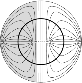
Figure 3. The overtwisted disk $\mathcal{D}_{ot}$ can be endowed with another characteristic foliation divided by the same dividing set (the thick circle). The foliation in the figure has a collection of singular points at the top and bottom of the boundary circle and on the horizontal diameter (near the endpoints and the center). A family of vertical leaves separates the right and the left half-disks. The vertical leaves go from singular points at the top (resp. bottom) of the boundary circle to singular points near the center. The right and left halves of the disk are foliated by arcs connecting singularities near the endpoints of the horizontal diameter and those near the center of $\mathcal{D}_{ot}$. The arcs located near $\partial\mathcal{D}_{ot}$ have vertical tangencies, thus the union of an arc on the top and the corresponding arc on the bottom (together with the singular points they connect) is a smooth Legendrian knot. The half-disk $D_{l}$ on the left side of $\mathcal{D}_{ot}$ is cut off by the leftmost vertical Legendrian arc.

Recall that the Thurston-Bennequin number of a Legendrian knot $K$ can be computed [Ho] from the dividing set $\Gamma_{\Sigma}$ on its convex Seifert surface $\Sigma$:

(1) $$\operatorname{tb}(K)=-\frac{1}{2}\,{\bigl{\lvert}\Gamma\cap K\bigr{\rvert}}\;.$$

From this formula, $\operatorname{tb}(\partial D_{l})=\operatorname{tb}(\partial D_{r})=-1$. Note that the Thurston-Bennequin number is defined even for piecewise smooth curves: indeed, linking with the transverse push-off is still well-defined. The formula (1) also holds in this context, which can be seen, for example, via approximation by smooth Legendrian curves. We will be attaching the overtwisted disk in two steps, first one half, that is, $D_{l}$, then the other, i.e. the Legendrian arcs and $D_{r}$. The idea is that half of $\mathcal{D}_{ot}$ is easier to control: indeed, half of an overtwisted disk represents a bypass, and bypasses can be found in tight contact manifolds [Ho].

Now we are ready to prove the theorem. Since the statement is local, it suffices to establish the claim for a small Legendrian unknot $L_{0}$ with $\operatorname{tb}(L_{0})=-1$, located near the overtwisted disk $\mathcal{D}_{ot}$ (and disjoint from it). Let $L$ be another standard Legendrian unknot with $\operatorname{tb}(L)=-1$, such that $L_{0}$ and $L$ together bound a thin annulus $A$ whose framing gives the Seifert framing on both knots, i.e. the contact framings of the knots are one less than the framings provided by the annulus. This property guarantees that after a small perturbation, we can assume $A$ to be convex. We will show that $L{\mathbin{\#}}\partial\mathcal{D}_{ot}$ is a destabilization of $L_{0}$. To begin, notice that the dividing set on $A$ consists of two parallel arcs, each connecting $L_{0}$ and $L$. To establish the theorem, we will show that the annulus $A{\mathbin{\#}}\mathcal{D}_{ot}$ bounded by $L_{0}$ and $L{\mathbin{\#}}\partial\mathcal{D}_{ot}$ can be perturbed into a convex surface with dividing set given by one boundary parallel arc with endpoints on $L_{0}$ (see Figure 4). This will be done in two steps.

2pt $L_{0}$ at 47 39 $L$ at 22 111 $\partial\mathcal{D}_{ot}$ at 179 90 $\Gamma$ at 91 87

Figure 4. Connected sum with the boundary of an overtwisted disk destabilizes a Legendrian knot.

First, assume that the part of $\partial\mathcal{D}_{ot}$ where the connected sum $L{\mathbin{\#}}\partial\mathcal{D}_{ot}$ was formed lies in $\partial D_{l}$, and consider the Legendrian connected sum $L{\mathbin{\#}}\partial D_{l}$. Make the annulus $A{\mathbin{\#}}D_{l}$ convex by a small isotopy fixing the boundary (we will keep the same notation for the perturbed surface). This is possible because $\operatorname{tb}$ of each boundary component is negative: $\operatorname{tb}(L_{0})=-1$ and $\operatorname{tb}(L{\mathbin{\#}}\partial D_{l})=\operatorname{tb}(L)+\operatorname{tb}(\partial D_{l})-1=-1$. Here, we are using [Ho, Proposition 3.1], where the convex perturbation is described as a two-stage process. First, a $C^{0}$-small isotopy is done near the Legendrian boundary of the surface to put a collar neighborhood of the boundary into standard form. Second, a $C^{\infty}$-small isotopy, supported away from the boundary, makes the surface convex. The first perturbation uses a model neighborhood of the Legendrian boundary, and introduces a certain number of singularities with uniform rotation of the contact structure between them. If a collar neighborhood for part of the boundary is already in standard form, this part can be kept fixed during the first isotopy. (A close examination of Honda’s proof shows that the same arguments go through in our case even though the boundary is only piecewise smooth. The key observation here is that the smooth Legendrian knots approximating the boundary of $D_{l}$ forms an annulus which is convex and in standard form in the terminology of [Ho, Proposition 3.1].) Therefore, we can assume that the isotopy that makes $A{\mathbin{\#}}D_{l}$ convex fixes a neighborhood of the diameter of $D_{ot}$ separating $D_{l}$ and $D_{r}$, more precisely, that all the straight Legendrian arcs between the two half-disks are kept fixed, as well as the half-disk $D_{r}$.

The convex surface $A{\mathbin{\#}}D_{l}$ (or rather, a surface with the same characteristic foliation) can be found in a tight contact manifold. Indeed, the dividing set on $D_{l}$ is the same as that on a bypass. Bypasses exist in tight contact manifolds, thus by Giroux Flexibility we can find a surface with foliation isomorphic to that on $D_{l}$. Furthermore, in a tight neighborhood of a bypass we can find both an annulus bounded by two small unknots and the strip needed to form the connected sum. Now, consider the dividing set $\Gamma$ on $A{\mathbin{\#}}D_{l}$. Tightness of a neighborhood of $A{\mathbin{\#}}D_{l}$ implies that $\Gamma$ can have no homotopically trivial closed components. By (1), $\Gamma$ intersects both components of the boundary of $A{\mathbin{\#}}D_{l}$ at two points. This gives the following possibilities for the dividing set: either (i) $\Gamma$ consists of two arcs, each connects a point on $L_{0}$ to a point on $L{\mathbin{\#}}\partial D_{l}$, or (ii) $\Gamma$ consists of two boundary-parallel arcs, plus possibly a number of closed curves running along the core of the annulus.

To rule out the second possibility, we argue as follows. Since $L_{0}$ is a small unknot, we can find a disk $U$ bounded by $L_{0}$, such that $U$ is contained in the tight neighborhood of the bypass $D_{l}$. We can assume that $U$ is convex; then its dividing set is given by a single arc connecting two points on $L_{0}$. Moreover, we can assume that $U\cup A{\mathbin{\#}}D_{l}$ is a convex surface (with a tight neighborhood). But then, if there is a boundary-parallel dividing curve on $A{\mathbin{\#}}D_{l}$ connecting two points of $L_{0}$, the surface $U\cup A{\mathbin{\#}}D_{l}$ would have a homotopically trivial closed component of the dividing set, which contradicts the tightness of the neighbourhood.

Once we know that on $A{\mathbin{\#}}D_{l}$ the dividing set $\Gamma$ consists of two parallel arcs running from $L_{0}$ to $L{\mathbin{\#}}\partial D_{l}$, it is clear that after we attach the other half of the overtwisted disk, the convex surface $A{\mathbin{\#}}\mathcal{D}_{ot}$ will have the dividing set as in Figure 4. In conclusion, the knot $L{\mathbin{\#}}\mathcal{D}_{ot}$ is a destabilization of $L$. ∎

3. Higher dimensions: definition of the plastikstufe

Many obstructions of fillability of higher dimensional contact manifolds have been found in the recent past [Ni1, MNW]. These obstructions are all modeled on the overtwisted disk and take the shape of particular submanifolds in the given contact manifold. The initial incarnation of this type of obstruction is the plastikstufe [Ni1]:

Definition 3.1.

Let $(M,\xi)$ be a contact manifold of dimension $2n+1$, and let $B$ be a closed $(n-1)$-manifold. A plastikstufe $\mathcal{P}_{B}$ with core $B$ is a submanifold

$$\mathcal{P}_{B}=D^{2}\times B\hookrightarrow M$$

such that $\xi\cap T\mathcal{P}_{B}$ is a singular foliation that is tangent to the fibers $\{z\}\times B$ for every $z\in D^{2}$, and that restricts on every slice $D^{2}\times\{b\}$ to the foliation of the overtwisted disk sketched in Figure 1. A plastikstufe $\mathcal{P}_{B}$ is called a small plastikstufe if there is an embedded open ball in $(M,\xi)$ containing $\mathcal{P}_{B}$. A contact manifold that contains a plastikstufe is called $PS$-overtwisted.

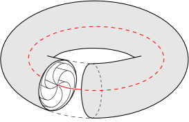
Figure 5. The core of a plastikstufe in a contact $5$-manifold is always a circle.

A plastikstufe determines the germ of the contact structure on its neighborhood [Ni2]. More precisely, let $\mathcal{D}_{ot}$ be an overtwisted disk in $\bigl{(}\mathbb{R}_{ot}^{3},\alpha_{ot}\bigr{)}$ with $\alpha_{ot}=\cos r\,dz+r\sin r\,d\varphi$ written in cylindrical coordinates. Then a plastikstufe $\mathcal{P}_{B}$ has a neighborhood $U_{PS}$ contactomorphic to a neighborhood of $\mathcal{D}_{ot}\times\{\text{0-section}\}$ in

$$\bigl{(}\mathbb{R}_{ot}^{3}\times T^{*}B,\alpha_{\mathrm{PS}}=\alpha_{ot}+{\lambda_{\mathrm{can}}}\bigr{)}$$

with ${\lambda_{\mathrm{can}}}=-{\boldsymbol{p}}\,d{\boldsymbol{q}}$ the canonical $1$-form on $T^{*}B$. (For purposes of the present paper, we could even accept the existence of a standard neighborhood of the plastikstufe as part of definition of a $PS$-overtwisted manifold.) In the next section, we will prove that Legendrians become flexible in the presence of a plastikstufe, at least if the latter satisfies some technical conditions.

4. $h$-principles, Legendrians, and plastikstufe

In this section, we review the definition of loose Legendrians and prove Theorem 1.1. We begin with some background on Gromov’s $h$-principle for Legendrian immersions [Gr, EM].

4.1. Formal homotopy of Legendrian immersions and Gromov’s $h$-principle

Observe that a Legendrian immersion $f\colon S\to(M,\xi)$ induces a monomorphism $df\colon TS\to TM$ such that $d_{x}f(T_{x}S)$ is a Lagrangian plane in the symplectic space $\bigl{(}\xi_{f(x)},d\alpha\bigr{)}$ for every $x\in S$. If we choose a compatible almost complex structure $J$ on $(M,\xi)$, then $d_{x}f(T_{x}S)$ is a totally real subspace in $\bigl{(}\xi_{f(x)},J\bigr{)}$. Thus, we can think of $df\colon TS\to\xi$ as Lagrangian monomorphism, or as a totally real monomorphism if an almost complex structure is chosen. (Note that in the latter case, the complexification $df^{\mathbb{C}}\colon T_{\mathbb{C}}S\to\xi_{f(x)}$ with $T_{\mathbb{C}}S=TS\otimes\mathbb{C}$ gives a complex isomorphism in every fiber.)

Suppose that $g,h\colon S\to M$ are two Legendrian immersions. If there is a regular homotopy of Legendrian immersions $f_{t}$ that connects $g$ and $h$, then the maps $dg\colon TS\to\xi$ and $dh\colon TS\to\xi$ are homotopic through $F_{t}=df_{t}$. Conversely, assume that

• there is a homotopy of continuous maps $f_{t}\colon S\to M$ connecting $g$ and $h$,

• and a homotopy $F_{t}$ of Lagrangian monomorphisms over $f_{t}$ connecting $dg,dh\colon TS\to\xi$.

In this case, we say that the Legendrian immersions $g$ and $h$ are formally homotopic. Gromov’s $h$-principle for Legendrian immersions implies that $g$ and $h$ are homotopic through Legendrian immersions whenever they are formally homotopic.

We also recall the definition of formal isotopy of isotropic embeddings. We say that isotropic embeddings $g,h\colon S\to M$ are formally isotopic if

• there is a smooth isotopy $f_{t}\colon S\to M$ of embeddings connecting $g$ and $h$;

• there is a homotopy $F_{t}$ of isotropic monomorphisms over $f_{t}$ connecting $dg,dh\colon TS\to\xi$;

• the path of isotropic monomorphisms $F_{t}$ is homotopic to $df_{t}$ through paths of monomorphisms with fixed endpoints $dg$, $dh$.

By a result of Gromov [Gr], formally isotopic subcritical isotropic embeddings are isotropically isotopic. The same holds for open Legendrian embeddings. In general, this $h$-principle fails for closed Legendrian embeddings, but it holds for the special class of loose Legendrians [Mu], which we review in the next subsection.

Remark 4.1.

The notion of formal homotopy carries over verbatim to the case where $\xi$ is an almost contact structure. Moreover, consider a path of almost contact structures $\xi_{t}$ that starts and ends at honest contact structures $\xi_{0}$ and $\xi_{1}$, respectively. Suppose that $f,g\colon S\to M$ are embeddings that are Legendrian for both $\xi_{0}$ and $\xi_{1}$, and the bundle maps $dg$ and $dh$ are Lagrangian for every almost contact structure $\xi_{t}$. Then $f$ and $g$ are formally homotopic with respect to $\xi_{0}$ if and only if they are formally homotopic with respect to $\xi_{1}$. In this case, Gromov’s $h$-principle implies that $f$ and $g$ are homotopic through immersions that are Legendrian with respect to $\xi_{0}$ if and only if they are homotopic through Legendrian immersions with respect to $\xi_{1}$.

Remark 4.2.

It is useful to reinterpret condition (b) in the definition of formal homotopy in different terms for the case where the image of Legendrian immersions $g,h\colon S\to M$ is contained in some open ball $U\subset M$. Fix a complex structure $J$ on $\xi$ that is tamed by the conformal symplectic structure given by ${\left.{d\alpha}\right|_{\xi}}$, and choose a $J$-complex trivialization of $(\xi,J)$ over the ball $U$; both $J$ and the trivialization will be unique up to homotopy. In particular, these choices allow us to identify $\bigl{(}{\left.{\xi}\right|_{U}},J\bigr{)}$ with the trivial bundle $\mathbb{C}^{n}\times U\to U$.

If $g\colon S\to(U,\xi)$ is a Legendrian immersion in $U$, we can write the differential $dg$ with respect to the trivialization chosen above, as a map $dg\colon TS\to\mathbb{C}^{n}$, and furthermore since $dg(T_{x}S)$ is a totally real subspace in $\bigl{(}\xi_{g(x)},J\bigr{)}$, the complexification

$$dg^{\mathbb{C}}\colon T_{\mathbb{C}}S\to\mathbb{C}^{n}$$

gives a complex isomorphism in every fiber.

Given now a second Legendrian immersion $h\colon S\to U$, we can relate the two maps $dg^{\mathbb{C}}$ and $dh^{\mathbb{C}}$ by a map $\varphi\colon S\to\operatorname{GL}(n,\mathbb{C})$ such that

(2) $$dh^{\mathbb{C}}_{x}=\varphi(x)\cdot dg^{\mathbb{C}}_{x}$$

for every $x\in S$. The homotopy class of $\varphi$ is called the relative rotation class of the Legendrian immersion $h$ relative to $g$. The relative rotation class is an element of $[S,\operatorname{GL}(n,\mathbb{C})]\cong[S,\operatorname{U}(n)]$. It is clear that the maps $dg^{\mathbb{C}}\colon TS\otimes\mathbb{C}\to\xi$ and $dh^{\mathbb{C}}\colon TS\otimes\mathbb{C}\to\xi$ are homotopic through fiberwise complex isomorphisms if and only if their relative rotation class vanishes.

4.2. Loose Legendrians

We define loose Legendrian embeddings [Mu] (or loose Legendrians for short) by requiring that they possess the following model chart.

Definition 4.3.

Let $n>1$. In $\bigl{(}\mathbb{R}^{3},\xi_{\mathrm{std}}=\ker(dz-y\,dx)\bigr{)}$, let $L_{0}$ be the Legendrian curve

$$t\mapsto\Bigl{(}t^{2},\frac{15}{4}\,(t^{3}-t),\frac{3}{2}t^{5}-\frac{5}{2}t^{3}\Bigr{)}\;,$$

where $t$ is in an open interval containing $[-\frac{\sqrt{5}}{\sqrt{3}},\frac{\sqrt{5}}{\sqrt{3}}]$. Let $U\subseteq\mathbb{R}^{3}_{\mathrm{std}}$ be some convex open set containing $L_{0}$ (see Figure 2). In $T^{*}\mathbb{R}^{n-1}$ let $Z$ be the Lagrangian zero section $\{\mathbf{p}=0\}$, and let $V_{\rho}$ be the open set $\bigl{\{}{\bigl{\lvert}\mathbf{p}\bigr{\rvert}}<\rho,{\bigl{\lvert}\mathbf{q}\bigr{\rvert}}<\rho\bigr{\}}$. Then $U\times V_{\rho}$ is canonically identified with an open set in $(\mathbb{R}^{2n+1},\xi_{\mathrm{std}})$, and $L_{0}\times Z$ is Legendrian in this contact Darboux chart. If $\rho>1$, we call the relative pair $(U\times V_{\rho},L_{0}\times Z)$ a loose chart. A connected Legendrian manifold $\Lambda\subseteq(M,\xi)$ with $\dim\Lambda>1$ is called loose if there is a Darboux chart $U\subseteq M$ so that $(U,\Lambda\cap U)$ is a loose chart.

Note that the above definition contains a size restriction $\rho>1$ on the chart parameter $\rho$. This is a key condition: indeed, any Legendrian can be shown to have a model chart with arbitrarily small $\rho$. It is not a priori clear why a chart with a small $\rho<1$ is not isomorphic to a chart with large $\rho>1$, but this must be true because loose Legendrians satisfy the following $h$-principle:

Theorem 4.4 ([Mu]).

If two loose Legendrians $\Lambda_{0},\Lambda_{1}$ in a contact manifold of dimension $2n+1>3$ are formally isotopic, then they are isotopic through Legendrian embeddings. ∎

In other words, loose Legendrians are flexible, i.e. they are classified up to Legendrian isotopy by easy to calculate invariants coming from smooth topology and bundle theory [Mu]. Recall that for general Legendrian embeddings, a similar $h$-principle manifestly does not hold in any dimension. It is known that holomorphic curve invariants detect Legendrian rigidity in many examples where two knots are formally isotopic but Legendrian non-isotopic. (This also tells us that the requirement $\rho>1$ imposes a non-trivial restriction.)

4.3. The proof of Theorem 1.1

Our strategy for proving Theorem 1.1 is quite simple. The motivation comes from Theorem 2.1: in every overtwisted $\mathbb{R}^{3}$-slice we can isotop a given Legendrian embedding of a knot to an embedding where its front projection has a “kink”. We can think of a plastikstufe as a “product” family of overtwisted disks and perform a family of the above isotopies for slices $\Lambda\cap\mathbb{R}^{3}\times\{b\}$ of a given Legendrian $\Lambda$ (near the plastikstufe). This product isotopy would produce a chart required by Definition 4.3 and verify that the given Legendrian is, indeed, loose. For us to carry out this plan, the Legendrian $\Lambda$, perhaps after an isotopy, must contain a codimension $0$ submanifold $\Lambda_{0}$ diffeomorphic to $B\times[0,1]$, where $B$ is the core of the plastikstufe $\mathcal{P}_{B}$. Moreover, $\Lambda_{0}$ must be in a “product position” in some standard neighborhood $U_{PS}=N_{\epsilon}\mathcal{D}_{ot}\times T_{\epsilon}^{*}B$ of $\mathcal{P}_{B}$:

$$\mathcal{P}_{B}= \mathcal{D}_{ot}\times\{\text{$0$-section}\} \subset U_{PS}\;,$$

$$\Lambda_{0}= K\times\{\text{$0$-section}\} \subset U_{PS}\;,$$

where $K\subset N_{\epsilon}\mathcal{D}_{ot}$ is a Legendrian arc. In other words, we must be able to move the given Legendrian $\Lambda$ by an ambient contact isotopy so that a product strip of the form $K\times\{\text{$0$-section}\}$ would be contained in $\Lambda$. In Lemma 4.7, we will show that this is possible if the plastikstufe has a spherical core and trivial rotation, a notion we now define.

A leaf ribbon in a plastikstufe $\mathcal{P}_{B}$ with core $B$ is a thin ribbon diffeomorphic to $B\times(0,1)$, obtained by shrinking a leaf of $\mathcal{P}_{B}$ within itself into the standard neighborhood of the core $B$. Notice that all such ribbons are Legendrian isotopic: ribbons contained in the same leaf are all deformations of the same leaf and ribbons in different leaves can be related by rotating around the binding.

From now on, we restrict to plastikstufes with core $B$ diffeomorphic to $S^{n-1}$ (see Remark 4.13 for a brief discussion of the general case). We will compare the formal Legendrian homotopy class of their leaf ribbons to the class represented by a punctured Legendrian disk.

Definition 4.5.

For a small plastikstufe $\mathcal{P}$ with spherical core, we define the rotation class of $\mathcal{P}$ to be the relative rotation class between a leaf ribbon of $\mathcal{P}$ and a punctured Legendrian disk. We say that $\mathcal{P}$ has trivial rotation if this class vanishes.

It is not hard to show that any two Legendrian disks in $(M,\xi)$ are Legendrian isotopic. Therefore, the rotation class of a small plastikstufes with spherical core is well-defined.

Remark 4.6.

The rotation class of a plastikstufe with core $B=S^{n-1}$ is an element of

$$\bigl{[}B\times[0,1],\operatorname{GL}(n,\mathbb{C})\bigr{]}\cong[B,\operatorname{U}(n)]=\pi_{n-1}(\operatorname{U}(n))=\begin{cases}\mathbb{Z}&\text{if $n$ is even}\\ 0&\text{if $n$ is odd.}\end{cases}$$

Thus, in contact manifolds of dimension $2n+1=4m+3$, every small plastikstufe with spherical core has trivial rotation. We will see in Subsection 4.4 that in the appropriate sense, the rotation of a plastikstufe in dimensions $2n+1=4m+1>5$ is determined by the rotation of its core, while in dimension $5$ it is the rotation of the leaf direction that determines the rotation of $\mathcal{P}$.

Given a plastikstufe $\mathcal{P}$ with trivial rotation, and a Legendrian $\Lambda$, we now isotop $\Lambda$ towards $\mathcal{P}$.

Lemma 4.7.

Suppose $(M^{2n+1},\xi)$ is $PS$-overtwisted and $\Lambda\subset M$ is a given Legendrian. Assume that there is a small plastikstufe $\mathcal{P}_{B}\subset(M,\xi)$ with spherical core $B=S^{n-1}$, and $\mathcal{P}$ has trivial rotation. Then there exists an ambient contact isotopy of $M$ that takes a submanifold $\Lambda_{0}$ of $\Lambda$ diffeomorphic to $S^{n-1}\times[0,1]$ to a product strip $\Lambda_{1}=K\times\{\text{$0$-section}\}$ near $\mathcal{P}_{B}$.

Proof.

We can assume that the plastikstufe $\mathcal{P}$ and at least some part of $\Lambda$ are contained in an open ball $U$. Fix a strip $\Lambda_{1}=S^{n-1}\times I$ which is isotopic to a leaf ribbon for $\mathcal{P}$ but lies in the complement of $\mathcal{P}$. (Here and below, $I$ denotes a closed interval.) Choose a small Legendrian disk in $\Lambda\cap U$, and let $\Lambda_{0}=S^{n-1}\times I$ be an annular Legendrian strip in this disk, so that the interior of $\Lambda_{0}$ is isotopic to the punctured disk.

Now we have two Legendrian embeddings $f_{0},f_{1}\colon S^{n-1}\times I\to M$, such that $\Lambda_{i}$ is the image of $f_{i}$, $i=0,1$. We would like to connect these by a path of Legendrian embeddings. We use Gromov’s $h$-principle for subcritical isotropic and open Legendrian embeddings [Gr], which in our situation works as follows.

We restrict attention to the core spheres $S_{i}=f_{i}\left(S^{n-1}\times\{c\}\right)$, $i=0,1$, where $c$ is a point inside $I$. (In what follows, we will be assuming that $c$ is close to an endpoint of $I$. It will be clear from the context where we want the core spheres to be; a particular choice is unimportant, since any two are isotropically isotopic.) Let ${\left.{f_{i}}\right|_{\text{core}}}\colon S^{n-1}\to M$ denote the isotropic embeddings given by the corresponding restriction maps. We first construct a formal isotropic isotopy between these embeddings.

Reparameterizing $I$, we can think of $f_{0}$ and $f_{1}$ as maps

$$f_{0}\colon S^{n-1}\times[0,\delta]\to M,\qquad f_{1}\colon S^{n-1}\times[1-\delta,1]\to M$$

for some small $\delta>0$. Choosing a trivialization of $\xi$ in $U$ as in Remark 4.2, we consider the maps

$$df_{0}^{\mathbb{C}}\colon T_{\mathbb{C}}(S^{n-1}\times[0,\delta])\to\mathbb{C}^{n},\qquad df_{1}^{\mathbb{C}}\colon T_{\mathbb{C}}(S^{n-1}\times[1-\delta,1])\to\mathbb{C}^{n}.$$

The map $df_{0}^{\mathbb{C}}$ is homotopic to the map $G^{\mathbb{C}}_{0}\colon T(S^{n-1}\times[0,\delta])\to\mathbb{C}^{n}$ defined by $G^{\mathbb{C}}_{0}(x,t)=df_{0}^{\mathbb{C}}(x,\delta)$, $0\leq t\leq\delta$. Similarly, $df_{1}^{\mathbb{C}}$ is homotopic to the map $G^{\mathbb{C}}_{1}\colon T(S^{n-1}\times[1-\delta,1])\to\mathbb{C}^{n}$ defined by $G^{\mathbb{C}}_{1}(x,t)=df_{1}^{\mathbb{C}}(x,1-\delta)$, $1-\delta\leq t\leq 1$. Then, we can write

(3) $$df_{0}^{\mathbb{C}}(x,\delta)=\psi(x)df_{1}^{\mathbb{C}}(x,1-\delta)$$

for a map $\psi\colon S^{n-1}\to\operatorname{GL}(n,\mathbb{C})$, cf. Remark 4.2.

Because $\mathcal{P}$ has trivial rotation and $\Lambda_{1}$ is isotopic to a leaf ribbon of $\mathcal{P}$, it follows that $\Lambda_{0}$ and $\Lambda_{1}$ are formally Legendrian homotopic. Then, the map $\psi$ is homotopic to the map sending each point of $S^{n-1}$ to the identity transformation in $\operatorname{GL}(n,\mathbb{C})$. Using this homotopy, we can construct a map

$$G^{\mathbb{C}}\colon T_{\mathbb{C}}(S^{n-1}\times[0,1])\to\mathbb{C}^{n}$$

which gives a complex isomorphism in every fiber and coincides with $df_{0}^{\mathbb{C}}$ near $S^{n-1}\times\{0\}$ and with $df_{1}^{\mathbb{C}}$ near $S^{n-1}\times\{1\}$. The real part $G$ of $G^{\mathbb{C}}$ is a Lagrangian monomorphism $T(S^{n-1}\times[0,1])\to\xi$, restricting to $df_{0}$ and $df_{1}$ near the ends of the cylinder $S^{n-1}\times[0,1]$.

The Smale-Hirsch immersion theorem (see e.g. [EM]) implies that $G$ is homotopic to the differential $dg$ of an immersion $g\colon{S^{n-1}\times[0,1]}\to M$ such that $g=f_{0}$ near $S^{n-1}\times\{0\}$ and $g=f_{1}$ near $S^{n-1}\times\{1\}$.

But $S^{n-1}\times[0,1]$ has dimension $n$, and $M$ has dimension $2n+1$, so we can perturb $g$ into general position by homotoping it (through immersions) to an embedding $\tilde{g}$. We can assume that this homotopy fixes the cylinder near the ends, and that the core spheres we took are close enough to the ends of the cylinder.

Clearly, the maps $\tilde{g}_{t}=\tilde{g}(\cdot,t)$ are smooth embeddings connecting ${\left.{f_{0}}\right|_{\text{core}}}$ and ${\left.{f_{1}}\right|_{\text{core}}}$. The maps $G_{t}={\left.{G(\cdot,t)}\right|_{T(S^{n-1}\times\{t\})}}$ are isotropic monomorphisms covering $\tilde{g}_{t}$; moreover, $G_{t}$ coincides with ${\left.{df_{0}}\right|_{TS^{n-1}}}$ resp. ${\left.{df_{1}}\right|_{TS^{n-1}}}$ near 0 resp. 1, and the path $G_{t}$ is homotopic to $d\tilde{g}$ rel endpoints. In short, we have a formal isotopy of subcritical isotropic embeddings. By Gromov’s $h$-principle, it follows that ${\left.{f_{0}}\right|_{\text{core}}}$ and ${\left.{f_{1}}\right|_{\text{core}}}$ can be connected by a path $\tilde{f}_{t}$ of isotropic embeddings.

The next step is to upgrade $\tilde{f}_{t}$ to a path of framed isotropic embeddings. For an $(n-1)$-dimensional isotropic submanifold $S$ of $(M^{2n+1},\xi)$, we consider a framing by a non-vanishing vector field $X\colon S\to\xi$, such that $X(s)\in(T_{s}S)^{\perp}\setminus T_{s}S$ for every point $s\in S$. (Here, $(T_{s}S)^{\perp}$ stands for the symplectic orthogonal complement of $T_{s}S$ in $(\xi,d\alpha)$; this subspace contains $T_{s}S$ and has dimension $n+1$.) In other words, we look at framings such that at every point of $S$ the direct sum $TS\oplus\operatorname{Span}(X)$ is a Lagrangian subspace of $\xi$. For an isotropic submanifold contained in a ball, we can use a trivialization to find two vector fields $v,v^{\prime}$ such that at every point $(T_{s}S)^{\perp}=T_{s}S\oplus\operatorname{Span}(v,v^{\prime})$, and think of the vector field $X$ as living in $\operatorname{Span}(v,v^{\prime})$. Since $X$ does not vanish, after normalizing we can think of the framing as a map $X\colon S\to S^{1}$.

Notice that the original embeddings $f_{0}$, $f_{1}$ of $S^{n-1}\times I$ endow the restrictions ${\left.{f_{i}}\right|_{\text{core}}}$, $i=0,1$ with a framing $X_{i}$ given by $X_{i}=df_{i}(\text{the $I$-direction})$. We would like to find framings $X_{t}$ for the isotropic embeddings $\tilde{f}_{t}$, so that the path $(\tilde{f}_{t},X_{t})$ connects $({\left.{f_{0}}\right|_{\text{core}}},X_{0})$ and $({\left.{f_{1}}\right|_{\text{core}}},X_{1})$. If $n>2$, then the maps $X_{0}\colon f_{0}(S^{n-1})\to S^{1}$ and $X_{1}\colon f_{1}(S^{n-1})\to S^{1}$ are necessarily homotopic, so we can find the desired path $X_{t}$. In the case $n=2$, recall that the differentials $df_{0}$ and $df_{1}$ of the embeddings of $S^{n-1}\times I$ were connected by a path of Lagrangian monomorphisms $F_{t}$. Then, $F_{t}(\text{the $I$-direction})$ is a homotopy between $X_{0}$ and $X_{1}$.

The framed isotropic isotopy of the core spheres $f_{0}(S^{n-1})$ and $f_{1}(S^{n-1})$ immediately gives a Legendrian isotopy of the original annuli $\Lambda_{0}$ and $\Lambda_{1}$. Indeed, $\Lambda_{0}$ and $\Lambda_{1}$ can be shrinked and flattened (by a Legendrian isotopy) to thin annuli around their core spheres, linear in the direction of $X_{0}$ resp. $X_{1}$. These can be connected by a family of thin Legendrian annuli built on the spheres $\tilde{f}_{t}(S^{n-1})$, spanning a linear strip in the $X_{t}$ direction. By the ambient isotopy theorem, (see e.g. [Ge, Theorem 2.6.2]), the resulting isotopy of Legendrian annuli can be realized by a compactly supported contact isotopy of $(M,\xi)$, concluding the proof. ∎

Lemma 4.8.

Suppose that $\Lambda$ is a Legendrian in $(M,\xi)$ which lies in the complement of a small plastikstufe with spherical binding and trivial rotation. Then there is an open subset $V$ of $M$ with topology $S^{n-1}\times D^{n+2}$ such that the pair $(V,V\cap\Lambda)$ is contactomorphic to $(D^{3}_{\mathrm{std}}\times D^{*}S^{n-1},\Lambda_{0})$, where $\Lambda_{0}$ is the cartesian product of a stabilization in $D^{3}_{\mathrm{std}}$ and the zero section in $D^{*}S^{n-1}$.

Proof.

By Lemma 4.7, after an appropriate Legendrian isotopy, in the standard neighborhood of the plastikstufe $\mathbb{R}^{3}_{OT}\times D^{*}S^{n-1}$ the Legendrian $\Lambda$ is given by $K\times S^{n-1}$. Our entire picture is $S^{n-1}$–equivariant, so we then apply Theorem 2.1 simultaneously for each point in $S^{n-1}$. ∎

Lemma 4.9.

Suppose that $\Lambda\subset(M,\xi)$ is Legendrian, and there exists an open set $V\subset M$ such that $(V,V\cap\Lambda)$ is contactomorphic to $(D^{3}_{\mathrm{std}}\times D^{*}S^{n-1},\Lambda_{0})$, where $\Lambda_{0}$ is the cartesian product of a stabilization in $D^{3}_{\mathrm{std}}$ and the zero section in $D^{*}S^{n-1}$. Then $\Lambda$ is loose.

Proof.

For any metric on $S^{n-1}$, $D^{*}S^{n-1}$ contains a subset symplectomorphic to $V_{\rho}=\bigl{\{}{\bigl{\lvert}{\mathbf{q}}\bigr{\rvert}}<\rho,\,{\bigl{\lvert}{\mathbf{p}}\bigr{\rvert}}<\rho\bigr{\}}\subset T^{*}\mathbb{R}^{n-1}$, for some $\rho$. Fix $\epsilon>0$ so that $\epsilon<\rho$. In $D^{3}_{\mathrm{std}}$, we can isotope any stabilization by compactly supported isotopy to the stabilization $\Lambda_{\epsilon}$ given by

$$t\mapsto\left(\epsilon t^{2},\frac{15\epsilon}{4}(t^{3}-t),\frac{\epsilon^{2}}{2}(3t^{5}-5t^{3})\right)\;.$$

This defines a subset $V$ of $(M,\xi)$ so that $(V,V\cap\Lambda)$ is contactomorphic to $(D^{3}_{\mathrm{std}}\times Q_{\rho},\Lambda_{\epsilon}\times Z)$, where $Z$ is the zero section in $Q_{\rho}$. Reparametrizing our coordinates by the contactomorphism $(x_{i},y_{i},z)\mapsto(\frac{x_{i}}{\epsilon},\frac{y_{i}}{\epsilon},\frac{z}{\epsilon^{2}})$ demonstrates that $V$ is a loose chart. ∎

4.4. Construction of small plastikstufes with trivial rotation.

For Theorem 1.1 to be useful, we need a supply of contact manifolds containing small plastikstufes satisfying the hypotheses of Lemma 4.7, i.e. having spherical core and trivial rotation. We will use the following result of Etnyre–Pancholi [EP] to find suitable examples.

Theorem 4.10 ([EP]).

Let $(M,\xi)$ be a contact manifold of dimension $2n+1$ and let $B$ be an $(n-1)$-dimensional isotropic submanifold with trivial conformal symplectic normal bundle. Then we may alter $\xi$ to a contact structure $\xi^{\prime}$ that contains a small plastikstufe with core $B$ such that $\xi$ and $\xi^{\prime}$ are homotopic through almost contact structures.

In fact, choosing any neighborhood $U$ of $B$, we can find a smaller neighborhood $U^{\prime}$ of $B$ such that both the modification and the homotopy only affect $\xi$ in $U\setminus\overline{U^{\prime}}$. ∎

In our application we need a refinement of this result, in which one also determines the rotation of the plastikstufe.

Proposition 4.11.

The modification of Theorem 4.10 can be applied in any contact manifold to produce a small plastikstufe with spherical core and trivial rotation.

Proof.

The only part of the statement which needs justification is that we can achieve triviality of the rotation class. Indeed, choose a Legendrian disk $D$ in $(M^{2n+1},\xi)$ and apply the construction from the proof of Theorem 4.10 to any cooriented codimension $1$ submanifold $B$ of $D$. This $B$ is automatically isotropic, and its symplectic normal bundle is spanned by $(X_{n},JX_{n})$ where $X_{n}$ denotes a vector field in $D$ that is transverse to $B$, and $J$ is a compatible almost complex structure on $\xi$. Since we can do this construction inside a small ball around the Legendrian disk $D$, the resulting contact structure $\xi^{\prime}$ will contain a small plastikstufe $\mathcal{P}_{B}$.

Assume for the rest of the proof that $B$ is a small sphere $S^{n-1}$ that bounds a Legendrian disk in $L$. (See Remark 4.13 below for discussion of the more general case.) By Remark 4.6, the rotation class of a small plastikstufe with spherical core necessarily vanishes in contact manifolds of dimension $4m+3$, but we still need to study the remaining dimensions $4m+1$. Below, we will first show that the rotation for any plastikstufe constructed by Theorem 4.10 (on a core $B=S^{n-1}$ that bounds a Legendrian disk before creating the plastikstufe) is trivial if $\dim M>5$. (This phenomenon already manifested itself in the proof of Theorem 1.1, where any two framings on isotropic spheres were automatically homotopic if $\dim M>5$.) Finally, we will show that using the Etnyre–Pancholi theorem 4.10 in dimension $5$ with more care, we can produce plastikstufes with arbitrary rotation class, including trivial rotation.

We can assume that the modification to $\xi^{\prime}$ has been done in a sufficiently small neighborhood of $S^{n-1}$ so that $\xi^{\prime}=\xi$ both close to the center of the auxiliary Legendrian disk $D$ chosen above, and outside of an embedded ball. Moreover, the Etnyre–Pancholi modification does not change the contact structure near the chosen isotropic submanifold $B$. Thus, close to $B$ the leaves of the resulting plastikstufe are also Legendrian with respect to the old contact structure $\xi$. Since $\xi$ and $\xi^{\prime}$ are homotopic, by Remark 4.1 it suffices to examine the rotation of a leaf with respect to $\xi$.

Choose a leaf ribbon near $B$ and compare its rotation to the punctured Legendrian disk $D-\{0\}\cong B\times I$. Recall that by Remark 4.2 we can trivialize $\xi$ over a ball containing the Legendrians, and then obtain the rotation class as the homotopy class of the map $\varphi\colon B\times I\to\operatorname{GL}(n,\mathbb{C})$ that satisfies Equation (2), where $h$ and $g$ denote the two embeddings we wish to compare. In fact, because $B\times I$ deformation retracts to $B$, it suffices to study the restriction of this map to $B\times\{1/2\}$.

Then the two embeddings are the same over $B$ and only differ in the remaining direction. Over $B$ the tangent bundle to the leaf ribbon splits as $TB\oplus\langle X_{l}\rangle$, where $X_{l}$ is the leaf direction, and the tangent bundle to the flat annulus splits as $TB\oplus\langle X_{n}\rangle$, where $X_{n}$ is the normal to $B$ in the disk $D$. Therefore, for any $q\in B$ we have

$$\varphi(q)=\begin{pmatrix}\mbox{\Huge${\mathrm{Id}}$}&\begin{array}[]{c}*\\ \vdots\\ \end{array}\\ 0\dotsb 0&\kappa(q)\end{pmatrix}$$

where $\kappa\colon B\to\mathbb{C}^{*}$ is a continuous function. This helps us understand the homotopy class of $\varphi$ in $[B,\operatorname{GL}(n,\mathbb{C})]$. We consider two cases.

Case 1. Suppose $2n+1>5$. Then the function $\kappa\colon B\to\mathbb{C}^{*}$ is homotopic to $1$, since by assumption $B=S^{n-1}$ with $n-1\geq 2$. It follows that $\varphi$ represents the trivial class in $[B,\operatorname{GL}(n,\mathbb{C})]$, so the plastikstufe $\mathcal{P}_{B}$ has trivial rotation.

Case 2. Suppose $2n+1=5$. Now, the function $\kappa$, and therefore $\varphi$, may represent a non-trivial homotopy class. It turns out that this class depends on the choice of coordinates in the Etnyre–Pancholi construction. A reparametrization will allow us to adjust the rotation class. To see this, we first review the setup of the construction of [EP]. Given an isotropic manifold $B$ with trivial symplectic conormal bundle, we use the isotropic neighborhood theorem to identify a neighborhood of $B$ in $(M,\xi)$ with $T^{*}B\times\mathbb{R}^{3}$, equipped with the contact form $p\,dq+dz+r^{2}\,d\theta$. Choosing a transverse curve $\gamma(t)$ in $\mathbb{R}^{3}$, we can further identify a neighborhood of $B\times\gamma$ in $T^{*}B\times\mathbb{R}^{3}$ with

$$\bigl{(}T^{*}B\times S^{1}\times D^{2},\ker(p\,dq+dt+r^{2}d\theta)\bigr{)}.$$

Here, $B$ is the $0$-section of $T^{*}B$, $p\,dq$ is the canonical $1$-form on $T^{*}B$, $S^{1}$ is the transverse curve $\gamma(t)$, and $D^{2}$ is an open disk with polar coordinates $(r,\theta)$. Since $\dim M=5$, we have $B=S^{1}$, and the coordinate $q$ varies in the unit circle. The generalized Lutz twist from the Etnyre–Pancholi construction produces in each of the slices $T^{*}B\times\{t_{0}\}\times D^{2}$ a plastikstufe $\mathcal{P}_{t_{0}}$ whose core is $B\times\{t_{0}\}$, where $B$ is the zero section as before. Near the core, the leaves of $\mathcal{P}_{t_{0}}$ are given by $\{\theta=\text{const}\}$.

We can define for any $a\in\mathbb{Z}$ a contactomorphism

$$F_{a}\colon T^{*}B\times S^{1}\times\mathbb{R}^{2}\to T^{*}B\times S^{1}\times\mathbb{R}^{2}$$

by $F_{a}(p,q,t,re^{i\theta})=\bigl{(}p-ar^{2},q,t,re^{i\,(\theta+aq)}\bigr{)}$ that preserves $p\,dq+dz+r^{2}\,d\theta$. Note that the zero section $\{p=0,r=0\}$ is preserved by $F_{a}$.

Instead of applying now the generalized Lutz twist of [EP] to the initial model neighborhood of $B$ we have chosen in the Legendrian disk $D$ above, we use first a restriction of the map $F_{a}$ to modify the coordinates of the model neighborhood. This means that for a fixed $t_{0}$, the construction will produce a plastikstufe with the same core for either choice of coordinates. The leaf direction near the binding, however, is different: we get $\{\theta=\text{const}\}$ for the plastikstufe $\mathcal{P}$ constructed with the old coordinates, and $\theta^{\prime}=\theta+aq=\text{const}$ for $\mathcal{P}^{\prime}$ constructed in the new coordinates. Intuitively, the leaf direction of $\mathcal{P}^{\prime}$ rotates $a$ times with respect to the leaf direction of $\mathcal{P}$ as we move around the circle $S^{1}=B$.

We now compute the relative rotation class between $\mathcal{P}$ and $\mathcal{P}^{\prime}$. For this, we compare two trivializations of the bundle $\xi\to B=S^{1}$ corresponding to the (Legendrian) leaves of our plastikstufes. With a choice of a compatible almost complex structure $J$ on $\xi$, each plastikstufe yields a trivialization of ${\left.{\xi}\right|_{B}}$ given by

$$\text{(core $S^{1}$-direction},J(\text{core $S^{1}$-direction}),\text{leaf direction},J(\text{leaf direction})).$$

Since the $S^{1}$-direction for $\mathcal{P}$ and $\mathcal{P}^{\prime}$ is the same and the leaf directions differ as described above, the two trivializations are related by the map $\varphi\colon S^{1}\to\operatorname{U}(2)$,

$$\varphi(q)=\begin{pmatrix}1&0\\ 0&2\pi iaq\end{pmatrix}.$$

Different values of $a$ give maps lying in different homotopy classes in $[S^{1},\operatorname{U}(2)]=\pi_{1}(\operatorname{U}(2))=\mathbb{Z}$. More precisely, we can realize any given element in $\pi_{1}(\operatorname{U}(2))$ by an appropriate choice of $a$. In particular, we can realize the class given by a flat Legendrian annulus (i.e. the one contained in the Legendrian disk $D$). It follows that by an appropriate choice of coordinates, we can construct a plastikstufe with trivial rotation class. ∎

Remark 4.12.

The previous proposition essentially shows that the Etnyre–Pancholi construction can be used to produce a plastikstufe with an arbitrary given rotation class. Indeed, any rotation class of the core can be realized by Gromov’s $h$-principle for subcritical isotropic embeddings. In the leaf direction, rotation is always trivial in dimensions higher than $5$; in dimension $5$, any given rotation can be realized by an appropriate choice of coordinates in the Etnyre–Pancholi construction. We leave the details to the reader as we have no use for plastikstufes with non-trivial rotation.

Remark 4.13.

The construction above could be generalize in a relatively easy way for a small plastikstufe $\mathcal{P}_{B}$ with core $B^{n-1}$, as long as $B^{n-1}$ can be (smoothly) embedded into $\mathbb{R}^{n}$. To simplify the presentation, we have chosen to restrict to the spherical case, pointing instead to Question 6.2.

5. Flexible Weinstein manifolds

Let $(W^{2n+2},d\lambda)$ be an exact symplectic manifold. Given an exhausting Morse function $\varphi\colon W\to\mathbb{R}$, we say the triple $(W,\lambda,\varphi)$ is a Weinstein manifold if the vector field $V$ determined by $V\,\lrcorner\,d\lambda=\lambda$ is gradient-like for the Morse function $\varphi$. (If $\varphi$ has finitely many critical points, we say that $W$ has finite type.) It follows that $\lambda$ is a contact form on any non-critical level set $\varphi^{-1}(c)$. Similarly, $(W,\lambda,\varphi)$ is a Weinstein cobordism from $(Y_{0},\xi_{0})$ to $(Y_{1},\xi_{1})$ if $\partial W=Y_{1}\cup-Y_{0}$, where $Y_{0}$ and $Y_{1}$ are level sets for $\varphi$, and $V$ points inwards along $Y_{0}$ and outwards along $Y_{1}$. If $Y_{0}=\emptyset$, $W$ is called a Weinstein domain.

Observe that because ${\mathcal{L}_{V}}\lambda=\lambda$, the flow of the vector field $V$ expands $\lambda$ exponentially. If $p\in W$ is a critical point of $\varphi$, the descending manifold $C$ of $p$ consists of all the points in $W$ which converge to $p$ by the flow of $V$. Since any vector in $TC$ converges to the zero vector at the point $p$ under the flow of $V$, but this flow also expands $\lambda$ exponentially, we conclude that ${\left.{\lambda}\right|_{C}}=0$. Thus any descending manifold is an isotropic submanifold of $W$, and furthermore it intersects every level set in a contact isotropic submanifold. In particular, every critical point of $\varphi$ must have index less than or equal to $n+1$.

A Weinstein cobordism of dimension $2n+2>4$ is called flexible if every descending manifold of index $n+1$ intersects the lower level sets along a loose Legendrian sphere (in other words, attaching spheres for all handles of index $n+1$ are loose Legendrians.) Here, we will assume for simplicity that all critical values of $\varphi$ are distinct. Using the $h$-principle result from [Mu], it is shown in  [CE] that flexible Weinstein cobordisms can be completely classified by their topology. There are several related theorem proved in [CE, Chapter 14]; we state two results (in the form relevant to our case).

Theorem 5.1 ([CE]).

Let $(W,\lambda,\varphi)$ be a flexible Weinstein cobordism from $(Y_{0},\ker\alpha_{0})$ to $(Y_{1},\ker\alpha_{1})$, such that $W$ is smoothly a product cobordism. Then after a homotopy through Weinstein structures, the cobordism $(W,\lambda,\varphi)$ is isomorphic to $(Y_{0}\times\mathbb{R},e^{t}\alpha_{0},t)$. In particular, $(Y_{0},\ker\alpha_{0})$ is contactomorphic to $(Y_{1},\ker\alpha_{1})$. ∎

Theorem 5.2 ([CE]).

Let $(W,\lambda_{0},\varphi_{0})$ and $(W,\lambda_{1},\varphi_{1})$ be two flexible Weinstein structures on a fixed manifold $W$. Suppose that $\omega_{0}=d\lambda_{0}$ and $\omega_{1}=d\lambda_{1}$ are homotopic through non-degenerate $2$-forms. Then there exists a homotopy of Weinstein structures connecting $(W_{0},\lambda_{0},\varphi_{0})$ and $(W_{1},\lambda_{1},\varphi_{1})$. ∎

Now we are ready to prove Theorem 1.2 from the Introduction:

Proof of Theorem 1.2.

We will prove the theorem under the assumption that hypothesis (2) is satisfied, i.e. $(Y_{0},\xi_{0})$ and $(Y_{1},\xi_{1})$ are the ends of a Stein cobordism $W$ smoothly equivalent to a product cobordism. As a first step we consider the induced Weinstein structure on the cobordism, and apply Theorem 5.1. (The proof that hypothesis (1) implies the isomorphism of the contact structures works in exactly the same way, except that we use Theorem 5.2 instead of Theorem 5.1).

Let $(M^{2n+1},\xi_{\mathrm{PS}})$ be a $PS$-overtwisted manifold containing a plastikstufe $\mathcal{P}$ satisfying the hypotheses of Theorem 1.1. By connect summing this manifold onto each level set of $W$ (away from all descending manifolds) we obtain a new Weinstein cobordism $\tilde{W}$ from $(Y_{0},\xi_{0}){\mathbin{\#}}(M,\xi_{\mathrm{PS}})$ to $(Y_{1},\xi_{1}){\mathbin{\#}}(M,\xi_{\mathrm{PS}})$. The cobordism $\tilde{W}$ has the same critical points as $W$, and each descending manifold is disjoint from $M$ (and in particular, from the plastikstufe $\mathcal{P}$) at every level set. By Theorem 1.1 this implies that all descending manifolds of index $n+1$ intersect all level sets in loose Legendrians, therefore $\tilde{W}$ is a flexible Weinstein cobordism. Since $\tilde{W}$ is smoothly equivalent to the product cobordism $(Y{\mathbin{\#}}M)\times[0,1]$, we can complete the proof by applying Theorem 5.1. ∎

6. Open questions

The questions in this section are not new, but with the results of this paper they may be formulated in a more precise way. Above we have showed that certain $PS$-overtwisted manifolds are flexible within the class of $PS$-overtwisted manifolds being Stein cobordant by a topologically trivial cobordism.

Question 6.1.

Even if the general flexibility question seems to be out of reach, it would be interesting to tackle more special cases. For example:

(a) Is it true that the connected sum of an Ustilovsky sphere (cf. [Us]) with a suitable $PS$-overtwisted manifold is contactomorphic to the $PS$-overtwisted manifold? Note that in this case, the two contact manifolds are cobordant via a topologically non-trivial Stein cobordism.

(b) Take a model $PS$-overtwisted sphere $(S^{2n+1},\xi_{PS})$. Is it true that $(S^{2n+1},\xi_{PS}{\mathbin{\#}}\xi_{PS})$ is contactomorphic to $(S^{2n+1},\xi_{PS})$?

Question 6.2.

Can we remove the technical conditions in Theorem 1.1 and prove similar statements for arbitrary plastikstufes, or, more generally, for arbitary bLobs? (Bordered Legendrian open books, or bLobs for short, were introduced in [MNW] to generalize the notion of $PS$-overtwistedness.)

It is not hard to see that the arguments of this paper go through in the presence of a “large” open ball in $\mathbb{R}^{3}_{ot}\times\mathbb{R}^{2n}$. Moreover, some properties of such ball [NP] resemble those of a loose chart. Is it true that a neighborhhood of an arbitrary plastikstufe or bLob contains such an open ball?

A further question is about finding the correct definition of overtwistedness in higher dimensions. A very useful approach to studying contact structures in all dimensions is provided by open book decompositions [Gi2].

Question 6.3.

Can our results be interepreted in terms of open books to obtain some type of flexibility in that context?

References

- [AS] M. Abouzaid and P. Seidel, Altering symplectic manifolds by homologous recombination, arXiv:1007.3281
- [CE] K. Cieliebak, Y. Eliashberg, Symplectic Geometry of Stein Manifolds, book to appear.
- [Dy] K. Dymara, Legendrian knots in overtwisted contact structures on , Ann. Global Anal. Geom. 19 (2001), 293–305.
- [E] Y. Eliashberg, Classification of overtwisted contact structures on -manifolds, Invent. Math. 98 (1989), no. 3, 623–637.
- [EF] Y. Eliashberg and M. Fraser, Topologically trivial Legendrian knots, J. Symplectic Geom. 7 (2009), no. 2, 77–127.
- [EM] Y. Eliashberg and N. Mishachev, Introduction to the -principle, Graduate Studies in Mathematics 48, American Mathematical Society (2002)
- [Et1] J. Etnyre, Legendrian and Transversal Knots, in the Handbook of Knot Theory (Elsevier B. V., Amsterdam), (2005) 105–185.
- [Et2] J. Etnyre, On knots in overtwisted contact structures, Journal of Quantum Topology, to appear, arXiv:1012.3745.
- [EP] J. Etnyre and D. Pancholi On generalizing Lutz twists, J. London Math. Soc. 84 (2011), no. 3, 670–688.
- [Ge] H. Geiges, An introduction to contact topology, Cambridge Studies in Advanced Mathematics 109, Cambridge University Press (2008).
- [Gi1] E. Giroux, Convexité en topologie de contact, Comment. Math. Helv. 66 (1991), no. 4, 637–677.
- [Gi2] E. Giroux, Géométrie de contact: de la dimension trois vers les dimensions supérieures, Proceedings of the International Congress of Mathematicians, Vol. II (2002), 405–414.
- [Gr] M. Gromov, Partial differential relations, Ergebnisse der Mathematik und ihrer Grenzgebiete (3), 9, Springer-Verlag (1986)
- [Ho] K. Honda, On the classification of tight contact structures. I, Geom. Topol. 4 (2000), 309–368.
- [MNW] P. Massot, K. Niederkrüger and C. Wendl, Weak and strong fillability of higher dimensional contact manifolds, Invent. Math. (2012), doi: 10.1007/s00222-012-0412-5
- [Mc] M. McLean, Lefschetz fibrations and symplectic homology, Geom. Topol. 13 (2009), 1877-–1944
- [Mu] E. Murphy, Loose Legendrian Embeddings in High Dimensional Contact Manifolds, arXiv:1201.2245.
- [Ni1] K. Niederkrüger, The plastikstufe – a generalization of the overtwisted disk to higher dimensions, Algebr. Geom. Topol. 6 (2006), 2473–2508.
- [Ni2] K. Niederkrüger, Habilitation, in preparation.
- [NP] K. Niederkrüger and F. Presas, Some remarks on the size of tubular neighborhoods in contact topology and fillability, Geom. Topol. 14 (2010), no. 2, 719–754.
- [Us] I. Ustilovsky, Infinitely many contact structures on , Internat. Math. Res. Notices 1999, no. 14, 781–791.
- [Vo] T. Vogel, Existence of Engel structures, Ann. of Math. (2) 169 (2009), no. 1, 79–137.