MIXED CONVECTION ABOVE A ROTATING DISK

Abstract

Mixed convection above a horizontal disk rotating in a semi-infinite fluid is examined when the disk is heated so that its temperature varies quadratically with distance away from its centre. Steady similarity solutions are presented for a range of values of the two dimensionless parameters, a Prandtl number and a Grashof number. The results are corroborated by asymptotic analyses undertaken in the limits of small and large Prandtl number. For finite Prandtl number, the existence of multiple solutions at fixed Grashof number is revealed. The similarity structure for steady solutions fails beyond a critical Grashof number and this is interpreted in terms of a finite-time singularity of the unsteady form of the governing equations.

1 Introduction

Free convection refers to the motion created by thermal effects in a fluid which is otherwise at rest. Forced convection refers to the situation in which an external flow field, such as a uniform stream, directly controls the movement and distribution of heat within a fluid. Of particular interest in the present work is the case of mixed convection in which free-convective effects interact directly with a forced convective motion.

In a typical free convection problem, buoyancy forces drive motion directly. This occurs, for example, when a heated plate is held inside a fluid in a vertical position. However, fluid motion may result from thermal buoyancy effects even when no component of the buoyancy force acts in the direction of the subsequent motion. Stewartson (1) and Gill et al. (2) demonstrated that free horizontal convection may occur in a boundary layer on a semi-infinite horizontal plate at a constant temperature. In this case there is no component of the buoyancy force in the direction of motion; rather the horizontal flow occurs indirectly as a result of a pressure gradient induced along the plate. Amin & Riley (3) demonstrated that horizontal free convection takes place above an infinite plate held in a quiescent fluid when the plate temperature varies along its length. This flow is also of boundary-layer type provided that the Grashof number, which measures the relative strength of the buoyancy-induced convection to viscous effects, is large.

In a study of mixed convection at a vertical plate held at a constant temperature, Merkin (4) showed that when the buoyancy force opposes the prevailing direction of motion, the boundary layer eventually separates and the solution fails at a singularity (akin to the classical Goldstein singularity in an isothermal boundary layer) where the skin friction vanishes. Similar singular behaviour and flow separation is seen for uniform flow past a flat plate with constant heat flux (5, 6), and a discussion of the character of the singularity at the separation point was provided by Hunt & Wilks (7). Jones (8) showed that for a heated semi-infinite plate inclined at a small negative angle to the horizontal, flow separation occurs without meeting a singularity, and it is possible to continue the integration of the boundary-layer equations downstream. The absence of a singularity may be attributed to the ability of the pressure-gradient to adjust interactively to accommodate the flow separation in a manner reminiscent of the interactive behaviour of the pressure-gradient required in traditional triple-deck theory (e.g. 9).

A number of mixed convection scenarios have been discussed in which a flow due to thermally-induced pressure gradient achieves a balance with a background flow field without provoking flow separation. Typically these have been described using similarity structures of the stagnation-point type which share many features with traditional boundary-layer theory but which do not formally require approximation on the assumption of a small dimensionless parameter. Amin & Riley (10) found that a steady solution may be constructed for mixed convection at a stagnation-point on a plane wall when the wall temperature gradient is assumed to vary quadratically with distance along the wall. Surprisingly a steady solution is possible not only when thermally-driven flow component is in the same direction as the background flow but also when it opposes the background flow. Arrieta-Sanagustín (11) considered the axisymmetric version of this problem and demonstrated that a steady solution is possible with the thermal flow opposing the stagnation-point flow provided that the Grashof number lies below a threshold value. Above this value the assumed similarity structure fails and an eruption of fluid from the vorticity layer adjacent to the wall is anticipated. Further examples are given by Revnic et al. (12), who examined mixed convection near a stagnation point on a vertical cylinder, and Merkin & Pop (13) who studied mixed convection at a vertical surface exposed to a far-field shear flow. In both cases steady solutions are available when the thermal flow reinforces the shear flow. Solutions also exist for an opposing thermal flow if a dimensionless mixed convection parameter is below a critical value. Finally we mention the very recent work of Riley (14), who examines the unsteady flow above a horizontal wall induced by a standing temperature wave.

In this paper we discuss mixed convection above a heated rotating disk. In the absence of a temperature field, the flow is described by a set of ordinary differential equations according to the classical three-dimensional stagnation-point structure of von Kármán (e.g. 15). Solutions of these equations have been studied exhaustively. Cochran (16) computed the most well-known solution, and that which is most commonly described in textbooks (e.g. 15, 17). More recently, a number of authors have pointed out the existence of multiple solutions. Zandbergen and Dijkstra (18) computed a second solution as part of a wider study which accounted for the effect of suction at the plate. Later, Lentini and Keller (19) showed that in fact there are an infinite number of solutions. An excellent survey of the results is given by Zandbergen and Dijkstra (20). In the presence of a temperature field, the flow can be analysed using the same von Kármán similarity structure with the additional assumption that the wall temperature varies quadratically with distance away from the centre of the disk. The mixed convection is characterised by two dimensionless parameters, a Prandtl number and a Grashof number. The rotation of the disk draws fluid downwards from infinity and forces it outwards away from the disk centre. For positive Grashof number, the thermally-induced pressure gradient opposes this and attempts to drive fluid towards the axis of rotation. For negative Grashof number, the thermally-induced pressure gradient complements the centrifugal flow. This case was studied by Sreenivasan (21).

Section 2 is devoted to steady solutions for a fixed Prandtl number, which are expected to exist when the Grashof number lies below a critical value. Moreover the non-uniqueness mentioned above for isothermal flow strongly suggests the presence of multiple solution branches for the heated flow problem, and this is indeed found to be the case. The steady solutions are investigated further in the limit of small and large Prandtl number in section 3. Above the critical Grashof number the solution to the unsteady, self-similar form of the governing equations encounters a finite time singularity, and this is explored numerically in section 4. Our findings are summarised in section 5.

2 Steady flow

We consider the steady flow generated by a combination of a horizontal, rotating flat plate and a thermally-induced radial pressure gradient. The flow is assumed to be incompressible and satisfy the Navier-Stokes equations under the Boussinesq approximation. The rotating plate boundary is located at $z^{*}=0$ and the fluid occupies the region $z^{*}>0$. The plate is assumed to rotate about the $z^{*}$ axis with angular velocity $\Omega\mathbf{k}$, where $\mathbf{k}$ is the unit vector in the positive $z^{*}$ direction. The flow is assumed to be axisymmetric with velocity components $u^{*},w^{*}$ in the $r^{*},z^{*}$ directions respectively and $v^{*}$ is the azimuthal velocity component. The pressure in the fluid is represented by $p^{*}$ and the temperature field in the fluid is represented by $\theta^{*}$. The plate temperature is assumed to vary quadratically with distance from the origin so that

$$\theta^{*}=\theta_{0}^{*}-\left(\frac{b}{\nu/\Omega}\right)(\theta_{0}^{*}-\theta_{\infty}^{*})\>r^{2}$$ (1)

at $z^{*}=0$, where $b$ is a positive dimensionless parameter, $\theta^{*}_{\infty}$ is the ambient temperature far from the plate and $\theta^{*}_{0}$ is the plate temperature at the origin.

We non-dimensionalize by writing

$$(r^{*},z^{*})=(\nu/\Omega)^{1/2}(r,z),\quad(u^{*},v^{*},w^{*})=\left(\nu\Omega\right)^{1/2}(u,v,w),$$ (2)

$$p^{*}=(\rho\nu\Omega)p,\quad\theta^{*}=\theta^{*}_{\infty}+(\theta^{*}_{0}-\theta^{*}_{\infty})\theta,$$ (3)

where $\nu$ is the kinematic viscosity. According to the Boussinesq approximation the fluid density is given by

$$\rho=\rho_{\infty}\Big{(}1-\beta(\theta^{*}_{0}-\theta^{*}_{\infty})\theta\Big{)},$$ (4)

where $\rho_{\infty}$ is the density attained at the ambient temperature $\theta_{\infty}^{*}$ and $\beta$ is the coefficient of thermal expansion far from the plate. The temperature field inside the fluid is governed by the dimensionless energy equation

$$\sigma(u\theta_{r}+w\theta_{z})=\theta_{rr}+\theta_{r}/r+\theta_{zz},$$ (5)

where $\sigma=\nu/\kappa$ is the Prandtl number and $\kappa$ is the thermal diffusivity of the fluid.

We seek a similarity solution of the form

$$u=ru_{0}(z),\quad v=rv_{0}(z),\quad w=w_{0}(z),\quad p=p_{0}(z)+r^{2}p_{1}(z),\quad\theta=\theta_{0}(z)+br^{2}\theta_{1}(z).$$ (6)

Substituting (6) into the Navier-Stokes equations we obtain

$$2u_{0}+\frac{\mbox{d}w_{0}}{\mbox{d}z} =0,$$ (7)

$$u_{0}^{2}-v_{0}^{2}+w_{0}\frac{\mbox{d}u_{0}}{\mbox{d}z} =-2p_{1}+\frac{\mbox{d}^{2}u_{0}}{\mbox{d}z^{2}},$$ (8)

$$2u_{0}v_{0}+w_{0}\frac{\mbox{d}v_{0}}{\mbox{d}z} =\frac{\mbox{d}^{2}v_{0}}{\mbox{d}z^{2}},$$ (9)

$$2u_{0}\theta_{1}+w_{0}\frac{\mbox{d}\theta_{1}}{\mbox{d}z} =\frac{1}{\sigma}\frac{\mbox{d}^{2}\theta_{1}}{\mbox{d}z^{2}}.$$ (10)

The boundary conditions are

$$u_{0}=0,\;v_{0}=1,\;w_{0}=0,\quad\theta_{1}=-1\quad\hbox{at}\quad z=0,$$ (11)

and

$$u_{0},\,v_{0},\,\theta_{1}\to 0\quad\hbox{as}\quad z\to\infty.$$ (12)

The pressure field $p_{1}$ is given by

$$p_{1}=-\mathrm{Gr}\int_{z}^{\infty}\theta_{1}\,\mathrm{d}z,$$ (13)

where the dimensionless Grashof number is defined to be

$$\mathrm{Gr}=\frac{\beta g(\theta_{0}^{*}-\theta_{\infty}^{*})}{\nu^{1/2}\Omega^{3/2}}.$$ (14)

The remaining unknown functions in (6), namely $p_{0}(z)$ and $\theta_{0}(z)$, satisfy a pair of ordinary differential equations, with accompanying boundary conditions, which can be written down in a straightforward manner. These are not the main focus of the present work, and so we do not give these here; our primary concern is with the system (7)-(13).

The problem is solved numerically by first truncating the infinite domain of integration at a finite level, $z_{\infty}$, and introducing a non-uniform grid covering the range $[0,z_{\infty}]$. In pratice it is useful to cluster grid points at $z=0$ in order to more accurately resolve the solution in the region close to the wall where variation is typically rapid. The equations are discretized using centered differences for the derivative terms at each interior grid point. The boundary conditions (11) are enforced at the first grid point and the conditions in (12) together with $p_{1}=0$ are enforced at the last grid point. The non-linear terms in the governing equations are dealt with using a quasi-linearization procedure as part of an iterative process. For example the term $u_{0}^{2}$ in (8) is replaced by $2u_{0}\tilde{u}_{0}-\tilde{u}_{0}^{2}$ where $\tilde{u}_{0}$ is the value from the previous iteration. In this way at each iteration we solve a tri-diagonal system of linear algebraic equations for the unknowns at each grid point. This is done efficiently using the Thomas algorithm (e.g. 22). The solution is deemed to have converged once the condition $|u_{0}-\tilde{u}_{0}|<\delta$ is met at every grid point for a prescribed choice of $\delta$. A similar convergence condition is required for all of the other flow variables. In practice we took $\delta=10^{-8}$. As a check, the converged numerical solution is substituted back into the governing equations.

When $\mathrm{Gr}=0$, so that thermal effects are absent, the problem reduces to the classical von Kármán rotating disk flow for which fluid is swept radially outwards along the plate and drawn down from infinity along the axis of rotation. For $\mathrm{Gr}>0$ a thermally-induced pressure gradient tends to force fluid radially inwards and up away from the plate. The presently sought similarity solution assumes that the magnitude of the vorticity decays with vertical distance upwards from the boundary. Its existence will be determined by a competition between the centrifugally-driven downwash, which tends to draw vorticity towards the boundary, and the thermally-driven upwash which tends to carry it away from the boundary. If $\mathrm{Gr}$ is sufficiently large we expect the latter to overcome the former and, consequently, for the hypothesised similarity structure to fail.

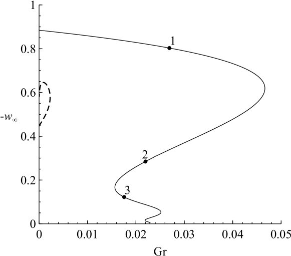
Figure 1: The steady solution curves for $\sigma=1$. The main branch is shown with a solid line, and one of the secondary branches is shown with a broken line. Velocity and temperature profiles at the points labelled 1, 2, 3 are shown in figures 2, 3 and 4 respectively.

As was mentioned in the Introduction, the presence of multiple solution branches is expected. In Fig. 1 we show two of the solution branches for the case $\sigma=1$. The flow is characterised using the negative of the vertical velocity at infinity, $w_{\infty}$. On both branches the solution at $\mathrm{Gr}=0$ was computed using the numerical method described above. The branches were then extended to positive Grashof numbers using the parameter continuation software AUTO-07p (23) with the finite difference solution at $\mathrm{Gr}=0$ used as a starting point. The branch shown with a solid line starts at the point $(\mathrm{Gr},w_{\infty})=(0,0.884)$, which coincides with the appropriate calculation of Zandbergen and Dijkstra (18) (see their table 4.1). The branch shown with a broken line starts at $(\mathrm{Gr},w_{\infty})=(0,0.447723)$, which also agrees with table 4.1 of Zandbergen and Dijkstra (18). As the branch extends away from $\mathrm{Gr}=0$ and starts to oscillate down toward the $\mathrm{Gr}$ axis, we found that it was necessary to gradually increase $z_{\infty}$ as the thickness of the vorticity layer at the disk grows. Over most of the branch we took $z_{\infty}=500$, but towards the lowermost part of the branch shown in the figure it was necessary to take the very large value $z_{\infty}=2\times 10^{4}$. For practical reasons, the computations were terminated at the end-point shown. It seems reasonable to suppose that the branch will continue to approach the $\mathrm{Gr}$ axis while the thickness of the vorticity layer continues to grow.

Having delineated the main branch as described, a few individual points along the branch were confirmed independently using an alternative numerical method as follows. The value of $w_{\infty}$ was fixed and $\mathrm{Gr}$ was treated as an unknown to come as part of the solution. Starting from the large $z$ asymptotic form of the solution provided by (18), (7)-(10) were integrated inwards from infinity, and a shooting method was used to satisfy the conditions at the disk (11). In each case the resulting pair $(\mathrm{Gr},-w_{\infty})$ was confirmed to lie on the main branch in Fig. 1.

On the main solution branch shown in Fig. 1, there is one solution when $0<\mathrm{Gr}<0.0156$, there are three solutions when $\mathrm{Gr}>0.0156$, and there are no solutions when $\mathrm{Gr}>\mathrm{Gr}_{c}$, where the critical Grashof number $\mathrm{Gr}_{c}=0.0466$. Velocity and temperature profiles at three locations on the main branch are shown in Figs 2, 3 and 4. Note that in the presently considered case of $\sigma=1$, it is readily seen from the governing equations (9) and (10) and the boundary conditions (11) and (12) that $v_{0}=-\theta_{1}$ and so the profile for the swirl component of velocity may be easily inferred from the temperature profiles shown in the figures. In each case the vertical velocity is single-signed and the fluid descends from infinity toward the disk. Notably, the radial velocity switches sign in the profiles shown in Figs 3 and 4 as a turning point develops in the axial $w_{0}$ profile. In Figs 2, 3, and 4, $\theta_{1}$, and hence also the swirl component $v_{0}$, has the same sign everywhere.

Other values of the Prandtl number, $\sigma$, were also investigated, and broadly the same behaviour was found as that discussed above. For example, the main solution branch was computed for the case $\sigma=0.5$ and it is found to be have qualitatively the same shape as that shown in Fig. 1. Fig. 5 shows how the critical Grashof number beyond which there are no steady solutions depends on the Prandtl number, $\sigma$. Notably, as $\sigma$ increases, $\mathrm{Gr}_{c}$ appears to grow without bound, and as $\sigma$ decreases, $\mathrm{Gr}_{c}$ appears to approach zero. These trends are investigated further in the next section where we examine the limits of large and small $\sigma$ in turn.

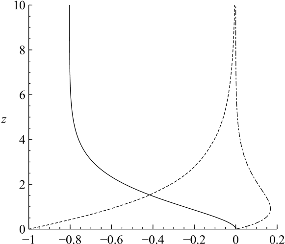
Figure 2: The velocity profiles $w_{0}$ (solid line), $u_{0}$ (dot-dashed line), and the temperature profile $\theta_{1}$ (dashed line) for $\sigma=1$ and $\mathrm{Gr}=0.0269$, corresponding to label 1 in figure 1 with $w_{\infty}=-0.803$. Note that for $\sigma=1$, as here, $v_{0}=-\theta_{1}$.

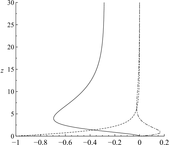
Figure 3: The velocity profiles $w_{0}$ (solid line), $u_{0}$ (dot-dashed line), and the temperature profile $\theta_{1}$ (dashed line) for $\sigma=1$ and $\mathrm{Gr}=0.0219$, corresponding to label 2 in figure 1 with $w_{\infty}=-0.284$. Note that for $\sigma=1$, as here, $v_{0}=-\theta_{1}$.

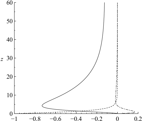
Figure 4: The velocity profiles $w_{0}$ (solid line), $u_{0}$ (dot-dashed line), and the temperature profile $\theta_{1}$ (dashed line) for $\sigma=1$ and $\mathrm{Gr}=0.0176$, corresponding to label 3 in figure 1 with $w_{\infty}=-0.122$. Note that for $\sigma=1$, as here, $v_{0}=-\theta_{1}$.

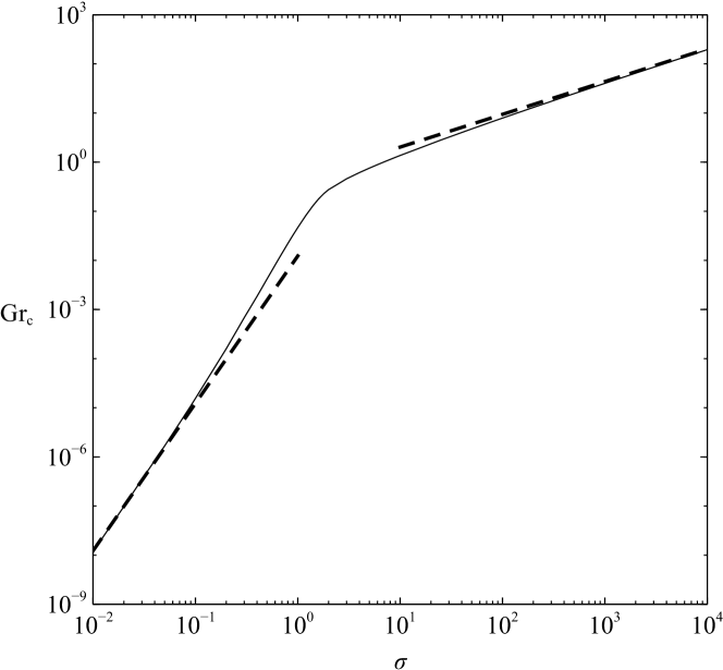
Figure 5: The dependence of the critical Grashof number, $\mathrm{Gr}_{c}$, on the Prandtl number $\sigma$, shown with a solid line. The broken lines correspond to the asymptotic predictions, $\mathrm{Gr}_{c}=0.436\sigma^{2/3}$ in (22) and $\mathrm{Gr}_{c}=0.0123\sigma^{3}$ in (38), for large and small $\sigma$ respectively.

3 Steady flow for large and small Prandtl number

Here we use asymptotic analysis to discuss the flow when $\sigma\gg 1$ and $\sigma\ll 1$. Of particular interest is the behaviour of the the critical Grashof number, $\mathrm{Gr}_{c}$, in these limits.

3.1 The case $\sigma\gg 1$

For large Prandtl number the diffusivity of heat from the boundary is much less than the diffusivity of vorticity created at the boundary. A consequence of this is that the thermal boundary layer is much thinner than the velocity boundary layer and so within the inner, thermal boundary layer the radial velocity is a linear function of $z$, i.e. $u_{0}\propto z$. A consequence is that if convection and diffusion of heat are to balance therein, (10) shows that the thickness of this inner layer is $O(\sigma^{-{1\over 3}})$, a classic result. Further $u_{0}=O(\sigma^{-{1\over 3}})$, and the continuity equation (7) requires $w_{0}=O(\sigma^{-{2\over 3}})$, with $v_{0}\equiv 1$ at leading order. A balance between the pressure and viscous forces in the radial momentum equation (8) then requires $p_{1}=O(\sigma^{1\over 3})$. Finally we note from equation (13) that Grashof numbers as large as $O(\sigma^{2\over 3})$ are available for steady flow in this situation. For this inner region then we introduce the scaled variables

$$u_{0}=\sigma^{-{1\over 3}}U_{0},\qquad w_{0}=\sigma^{-{2\over 3}}W_{0},\qquad p_{1}=\sigma^{1\over 3}P_{1},\qquad Gr=\sigma^{2\over 3}\Lambda,\qquad z=\sigma^{-{1\over 3}}Z,$$ (15)

which yield the following equations for the inner layer

$$2U_{0}+\frac{\mbox{d}W}{\mbox{d}Z}=0,\qquad 0=-2P_{1}+\frac{\mbox{d}^{2}U_{0}}{\mbox{d}Z^{2}},$$ (16)

$$2U_{0}\theta_{1}+W_{0}\frac{\mbox{d}\theta_{1}}{\mbox{d}Z}=\frac{\mbox{d}^{2}\theta_{1}}{\mbox{d}Z^{2}},\qquad\frac{\mbox{d}P_{1}}{\mbox{d}Z}=\Lambda\theta_{1},$$ (17)

with boundary conditions

$$U_{0}=W_{0}=0,\quad\theta_{1}=-1\quad\hbox{at}\quad Z=0,\quad P_{1},\theta_{1}\to 0\quad\hbox{as}\quad Z\to\infty,$$ (18)

together with a suitable matching condition for $U_{0}$ as $Z\to\infty$.

Outside this thin thermal boundary layer $p_{1}=\theta_{1}=0$ and the velocity components are each of order unity. Therefore, the governing equations for the outer layer, whose characteristic thickness is of order unity, are from (7) to (9)

$$2u_{0}+\frac{\mbox{d}w_{0}}{\mbox{d}z}=0,\quad u_{0}^{2}-v_{0}^{2}+w_{0}\frac{\mbox{d}u_{0}}{\mbox{d}z}=\frac{\mbox{d}^{2}u_{0}}{\mbox{d}z^{2}},\quad 2u_{0}v_{0}+w_{0}\frac{\mbox{d}v_{0}}{\mbox{d}z}=\frac{\mbox{d}^{2}v_{0}}{\mbox{d}z^{2}},$$ (19)

together with

$$u_{0}=v_{0}-1=w_{0}=0\quad\hbox{at}\quad z=0,\quad u_{0},v_{0}\to 0\quad\hbox{as}\quad z\to\infty.$$ (20)

Therefore the flow in this outer layer corresponds to the classical von Kármán rotating disk flow. In order to match the inner and outer solutions note from (16) that as $Z\to\infty$, $U_{0}\propto Z$. Accordingly, taking account of the scalings in (15), the matching requirement is

$$\left.\frac{\mbox{d}U_{0}}{\mbox{d}Z}\right|_{Z\to\infty}=\left.\frac{\mbox{d}u_{0}}{\mbox{d}z}\right|_{z=0}.$$ (21)

The system of equations (16) to (18) has been integrated numerically using the method outlined in section 2 for varying values of $\Lambda$. In particular we find that no solutions exist for $\Lambda=\Lambda_{c}>0.436$. Therefore the asymptotic behaviour of the critical Grashof number for large values of the Prandtl number has

$$\mathrm{Gr}_{c}\sim 0.436\sigma^{2\over 3}\quad\hbox{as}\quad\sigma\to\infty.$$ (22)

This result is compared with the results obtained from the numerical solutions of (7) to (13) in Fig. 5, showing good agreement for large values of $\sigma$.

3.2 The case $\sigma\ll 1$

For very small values of the Prandtl number, the thermal diffusivity is much greater than the diffusivity of vorticity, with the consequence that the thermal boundary layer now exceeds, by far, the velocity boundary layer in thickness. Assuming, as is reasonable, that the range of available values of $\mathrm{Gr}$ is small (see Fig. 5) in the inner region, where $z=O(1)$, we have from (7)-(10), at leading order

$$2\tilde{u}_{0}+\frac{\mbox{d}\tilde{w}_{0}}{\mbox{d}z}=0,\quad\tilde{u}^{2}_{0}-\tilde{v}^{2}_{0}+\tilde{w}_{0}{\mbox{d}\tilde{u}_{0}\over\mbox{d}z}={\mbox{d}^{2}\tilde{u}_{0}\over\mbox{d}z^{2}},\quad 2\tilde{u}_{0}\tilde{v}_{0}+\tilde{w}_{0}{\mbox{d}\tilde{v}_{0}\over\mbox{d}z}={\mbox{d}^{2}\tilde{v}_{0}\over\mbox{d}z^{2}},$$ (23)

together with

$$\tilde{u}_{0}=\tilde{v}_{0}-1=\tilde{w}_{0}=0\quad\hbox{at}\quad z=0,\quad\tilde{u}_{0},\tilde{v}_{0}\to 0$$ (24)

as $z\to\infty$. Notice that we have used a tilde superscript to indicate variables in the inner region. System (23), (24) is uncoupled from the temperature field and is identical to that which governs classical von Kármán flow over a rotating disk. The solution has the property that $\tilde{w_{0}}\to-k$ as $z\to\infty$, where $k=0.884$ (e.g. (20), table 4.1), and $\tilde{u}_{0}$, $\tilde{v}_{0}\to 0$ exponentially fast.

In the outer thermal boundary layer, we expect a balance between the outward diffusion and the inward convection of heat so that in (10)

$${\mbox{d}^{2}\theta_{1}\over\mbox{d}z^{2}}\sim\sigma w_{0}\frac{\mbox{d}\theta_{1}}{\mbox{d}z}=O\left(\sigma k{\mbox{d}\theta_{1}\over\mbox{d}z}\right).$$ (25)

This suggests that the aforementioned balance occurs in a region of scale $O(\sigma^{-1})$ which prompts the definition of an outer variable $\zeta=\sigma z$. Written in terms of the new outer variable, (8) and (13) become respectively,

$$u^{2}_{0}-v^{2}_{0}-\sigma k{\mbox{d}u_{0}\over\mbox{d}\zeta}=-2p_{1}+\sigma^{2}{\mbox{d}^{2}u_{0}\over\mbox{d}\zeta^{2}},\qquad\frac{\mbox{d}p_{1}}{\mbox{d}\zeta}=\frac{\mathrm{Gr}}{\sigma}\,\theta_{1}.$$ (26)

The first of these suggests viscous diffusion is unimportant and, balancing the three momentum terms on the left hand side with the pressure term on the right hand side, indicates that $u_{0}=O(\sigma)$, $v_{0}=O(\sigma)$ and $p_{1}=O(\sigma^{2})$ in this outer region. Substituting the last of these scalings into the second equation in (26), and assuming that $\theta_{1}=O(1)$, we deduce that $\mathrm{Gr}=O(\sigma^{3})$. Accordingly we now write $\mathrm{Gr}=\lambda\sigma^{3}$ where $\lambda=O(1)$ and seek to determine the critical value of $\lambda$ beyond which there is no steady solution.

With the above preliminaries in place we now develop the solution in greater detail. In the inner region we expand the velocity, pressure and temperature fields by writing

$$u_{0}=\tilde{u}_{0}+\sigma\tilde{u}_{1}+\sigma^{2}\tilde{u}_{2}+\cdots,\qquad v_{0}=\tilde{v}_{0}+\sigma\tilde{v}_{1}+\sigma^{2}\tilde{v}_{2}+\cdots,$$

$$w_{0}=\tilde{w}_{0}+\sigma\tilde{w}_{1}+\sigma^{2}\tilde{w}_{2}+\cdots,\qquad p_{1}=\sigma^{2}\tilde{p}_{0}+\cdots,\qquad\theta_{1}=\tilde{\theta}_{1}+\sigma\tilde{\theta}_{2}+\cdots.$$ (27)

Introducing these expansions into (7)-(10) we obtain (23) at leading order for which, as was mentioned above, the classical von Kármán solution is available. The leading order temperature field satisfies

$$\frac{\mbox{d}^{2}\tilde{\theta}_{1}}{\mbox{d}z^{2}}=0,$$ (28)

with $\tilde{\theta}_{1}=-1$ on $z=0$. Integrating and applying the wall boundary condition we find $\tilde{\theta}_{1}=-1+Az$ for constant $A$. We find that a self-consistent solution can be constructed by taking $A=0$ so that $\tilde{\theta}_{1}=-1$. At first order, namely $O(\sigma)$, we obtain from (7) and (8) respectively,

$$2\tilde{u}_{1}+{\mbox{d}\tilde{w}_{1}\over\mbox{d}z}=0,\quad 2\tilde{u}_{0}\tilde{u}_{1}-2\tilde{v}_{0}\tilde{v}_{1}+\tilde{w}_{0}{\mbox{d}\tilde{u}_{1}\over\mbox{d}z}+\tilde{w}_{1}{\mbox{d}\tilde{u}_{0}\over\mbox{d}z}={\mbox{d}^{2}\tilde{u}_{1}\over\mbox{d}z^{2}},$$ (29)

and from (9) we have

$$2\tilde{u}_{0}\tilde{v}_{1}+2\tilde{u}_{1}\tilde{v}_{0}+\tilde{w}_{0}{\mbox{d}\tilde{v}_{1}\over\mbox{d}z}+\tilde{w}_{1}{\mbox{d}\tilde{v}_{0}\over\mbox{d}z}={\mbox{d}^{2}\tilde{v}_{1}\over\mbox{d}z^{2}}.$$ (30)

At the wall we have $\tilde{u}_{1}=\tilde{v}_{1}=\tilde{w}_{1}=0$. Taking the limit $z\to\infty$, and considering the dominant balances of terms in (29), (30) we find

$$\tilde{u}_{1}\sim\alpha_{1}+\mbox{e.d.t.}\qquad\tilde{w}_{1}\sim-2\alpha_{1}z+\alpha_{2}+\mbox{e.d.t.},\qquad\tilde{v}_{1}\sim\alpha_{3}+\mbox{e.d.t.}$$ (31)

as $z\to\infty$, where e.d.t. means ‘exponentially decaying terms’ and $\alpha_{1}$, $\alpha_{2}$, and $\alpha_{3}$ are constants.

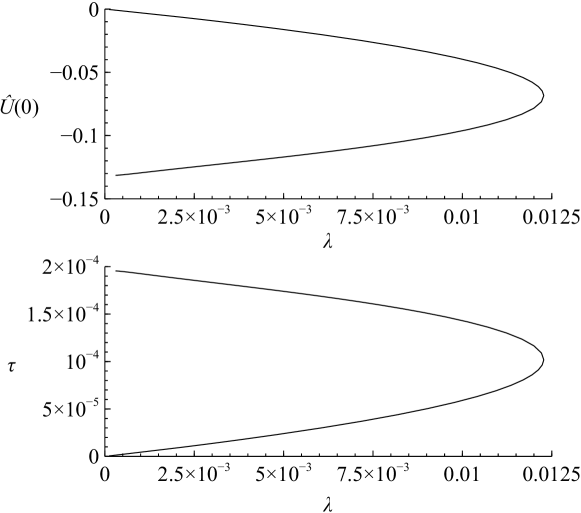
Figure 6: $\sigma\ll 1$: The solution branches for the first order problem in the inner region (lower panel, showing $\tau\equiv\mbox{d}\tilde{u}_{1}/\mbox{d}z|_{z=0}$) and the leading order problem in the outer region (upper panel, showing $\hat{U}(0)$).

In the outer region, we expand by writing

$$u_{0}=\sigma\>\hat{U}(\zeta)+\cdots,\qquad v_{0}=\sigma\>\hat{V}(\zeta)+\cdots,\qquad w_{0}=\hat{W}(\zeta)+\cdots,$$ (32)

$$p_{1}=\sigma^{2}\>\hat{P}(\zeta)+\cdots,\qquad\theta_{1}=\hat{\Theta}(\zeta)+\cdots,$$ (33)

where $\zeta=\sigma z$. Substituting into (7)-(10) and (13) we obtain at leading order,

$$2\hat{U}+{\mbox{d}\hat{W}\over\mbox{d}\zeta}=0,\qquad \hat{U}^{2}-\hat{V}^{2}+\hat{W}{\mbox{d}\hat{U}\over\mbox{d}\zeta}=-2\hat{P},$$ (34)

$$2\hat{U}\hat{V}+\hat{W}{\mbox{d}\hat{V}\over\mbox{d}\zeta}=0,\qquad {\mbox{d}\hat{P}\over\mbox{d}\zeta}=\lambda\hat{\Theta},\qquad 2\hat{U}\hat{\Theta}+\hat{W}{\mbox{d}\hat{\Theta}\over\mbox{d}\zeta}={\mbox{d}^{2}\hat{\Theta}\over\mbox{d}\zeta^{2}},$$ (35)

together with

$$\hat{W}(0)=-k,\quad\hat{\Theta}(0)=-1,\quad\hbox{and}\quad\hat{U},\hat{V},\hat{P},\hat{\Theta}\to 0\quad\hbox{as}\quad\zeta\to\infty.$$ (36)

The first two conditions in (36) are required to match to the inner region. Moreover, matching is completed by taking

$$\alpha_{1}=\hat{U}(0),\qquad\alpha_{3}=\hat{V}(0).$$ (37)

Integrating the first equation in (35), with the use of the first equation in (34), we find that $\hat{V}=-(\alpha_{3}/k)\hat{W}$, where the constant of integration has been chosen to fulfil the matching condition in (37). Substituting this result, the system (34)-(36) is solved numerically using a shooting method based on fourth-order Runge-Kutta integration. The numerical solution shows that $\alpha_{3}=0$ so that $\hat{V}\equiv 0$. The numerical solution is illustrated in the upper panel of Fig. 6, where $\hat{U}(0)$ is plotted against $\lambda$. Evidently two possible solutions exist over the range of $\lambda$ values shown, and there is no solution beyond the critical value $\lambda_{c}=0.0123$. The lower panel of the same figure shows the corresponding solution branch, showing $\mbox{d}\tilde{u}_{1}/\mbox{d}z|_{z=0}$ versus $\lambda$, for the first order inner system (29)-(31). It should be noted that while the solution for the swirl component $\hat{V}$ is identically zero in the upper region, the inner solution $\tilde{v}_{1}$ varies smoothly from zero at $z=0$, through non-zero values, toward zero as $z\to\infty$. According to the preceding remarks, we now have the asymptotic estimate for the critical Grashof number,

$$\mathrm{Gr}_{c}\sim 0.0123\sigma^{3}\quad\hbox{as}\quad\sigma\to 0.$$ (38)

This is compared with the critical value of the Grashof number obtained from the full equations in Fig. 6, showing excellent agreement.

In concluding this section it is worth reflecting on the rather unexpected flow structure which has been uncovered. First, we highlight the somewhat surprising form of the inner layer expansions (27). As was noted above, the leading order velocity field, namely $(\tilde{u}_{0},\>\tilde{v}_{0},\>\tilde{w}_{0})$, coincides with that for classical von Kármán flow on a rotating disk. Deviation from this basic profile occurs as a result of a thermally-induced pressure gradient which arises from the spatially-dependent wall temperature profile. It is notable that although this thermally-induced pressure gradient appears at $O(\sigma^{2})$ in the inner region expansions (27), it is necessary to include velocity perturbations of size $O(\sigma)$. These velocity perturbations are driven indirectly by thermal effects via the radial slip velocity which is imposed upon the inner layer by the solution in the outer region, where the effect of a thermally-induced pressure-gradient is felt at leading order. Finally we note that the present flow structure is similar in vein to that uncovered by Riley (14) in his study of the flow response of a semi-infinite fluid above a horizontal wall with a standing wave temperature profile.

4 Time-dependent calculations

Following the remarks of the previous section, it appears that no steady solution exists when the Grashof number lies above a critical value, $\mathrm{Gr}_{c}$, which depends on the size of the Prandtl number. To explore the flow behaviour above the critical Grashof number, we consider the unsteady form of the governing equations (7)-(13) with the time-dependent terms included,

$$2u_{0}+\frac{\partial w_{0}}{\partial z} =0,$$ (39)

$$\frac{\partial u_{0}}{\partial t}+u_{0}^{2}-v_{0}^{2}+w_{0}\frac{\partial u_{0}}{\partial z} =-2p_{1}+\frac{\partial^{2}u_{0}}{\partial z^{2}},$$ (40)

$$\frac{\partial v_{0}}{\partial t}+2u_{0}v_{0}+w_{0}\frac{\partial v_{0}}{\partial z} =\frac{\partial^{2}v_{0}}{\partial z^{2}},$$ (41)

$$\frac{\partial\theta_{1}}{\partial t}+2u_{0}\theta_{1}+w_{0}\frac{\partial\theta_{1}}{\partial z} =\frac{1}{\sigma}\frac{\partial^{2}\theta_{1}}{\partial z^{2}},$$ (42)

where $t=\Omega t^{*}$ is a dimensionless time, together with (13). These are to be integrated forwards in time subject to the boundary conditions (11) and (12). A suitable initial condition is given by

$$u_{0}=-\frac{1}{2}\frac{\mbox{d}F}{\mbox{d}z},\qquad v_{0}=G,\qquad w_{0}=F,\qquad\theta_{1}=p_{1}=0$$ (43)

at $t=0$, where the functions $F(z)$ and $G(z)$ are Cochran’s (16) solution to (7)-(9) at $\mathrm{Gr}=0$. We note that the same initial condition was used by Riley (24, 25) and Andrews and Riley (26) in their studies of heat transfer on a rotating disk.

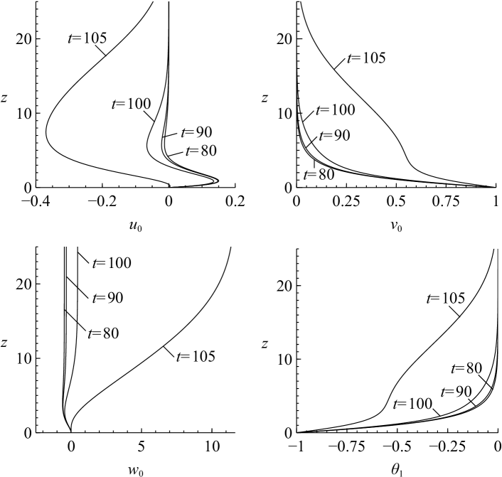
Figure 7: Velocity and temperature profiles $u_{0}$, $v_{0}$, $w_{0}$, and $\theta_{1}$ at various dimensionless times for $\sigma=1$ and $\mathrm{Gr}=0.05$.

The integration forwards in time may be achieved numerically employing a Crank-Nicolson scheme based on the same discretisation of the equations as in Bodonyi and Stewartson (27). The nonlinear terms are dealt with at each time step using an iterative method similar to that described by Tanehill et al. (28). A uniform time-step of size $0.01$ was used for the Crank-Nicolson scheme, whereas the same spatial discretization as described in section 2 was employed.

As in the previous section we focus attention on the case $\sigma=1$. The velocity and temperature profiles $u_{0}$, $v_{0}$, $w_{0}$ and $\theta_{1}$ are shown in Fig. 7 at different times $t$. Similar behaviour is encountered at other Grashof numbers above the critical value. In the early part of the flow evolution, the majority of the vorticity is confined to a layer adjacent to the disk. As time increases, the thickness of this layer increases as vorticity spreads further and further from the disk; this is evident from the behaviour of the $v_{0}$ curves in Fig. 7, which approach zero further and further from the disk as time goes on. Eventually, the numerical evidence is that a finite-time singularity is encountered and the solution blows up (in this case at $t\approx 107$). This singular behaviour lends strong support to the assertion that no steady solution exists above the critical value of the Grashof number discussed in section 2.

5 Summary

We have studied mixed convection over a rotating disk with the flow driven in part by the rotation of the disk and in part by a thermally-induced pressure gradient which arises in response to a prescribed temperature profile in the disk. Working on the basis of the Boussinesq approximation, we derived a set of partial differential equations describing the flow and the temperature profile throughout the fluid according to an assumed similarity structure. Steady solutions of this system are possible when the dimensionless Grashof number lies below a critical value which depends on the size of the Prandtl number. Below the critical Grashof number, an infinite number of solution branches exist, each one stemming from one of the infinity of branches which exist at zero Grashof number for isothermal flow. The main solution branch, which stems from the well-known Cochran solution of the classical von Kármán problem at zero Grashof number, undergoes a number of successive turns so that multiple steady solutions exist along this branch alone. Asymptotic descriptions of the flow, and in particular estimates for the critical Grashof number, were obtained in the limit of large and small Prandtl numbers and shown to be in agreement with the numerical computations. Beyond the critical Grashof number there are no steady solutions; rather, our unsteady calculations suggest that the solution of the unsteady similarity equations, subject to a suitable initial condition, terminates in a finite-time singularity.

References

- (1) K. Stewartson, On the free convection from a horizontal plate. Z. angew. Math. Phys. 9 (1958) 276-282.
- (2) W. N. Gill, D. W. Zeh and E. Del Casal, Free convection on a horizontal plate. Z. angew. Math. Phys. 16 (1965) 539-541.
- (3) N. Amin and N. Riley, Horizontal free convection. Proc. R. Soc. Lond. A 427 (1990), 371-384.
- (4) J. H. Merkin, The effect of buoyancy forces on the boundary-layer flow over a semi-infinite vertical flat plate in a uniform stream. J. Fluid Mech. 35 (1969) 439-450.
- (5) G. Wilks, A separated flow in mixed convection. J. Fluid Mech. 62 (1974) 359-368.
- (6) G. Wilks, The flow of a uniform stream over a semi-infinite vertical flat plate with uniform surface heat flux, Int. J. Heat Mass Transf. 17 (1974) 743-753.
- (7) R. Hunt and G. Wilks, On the behaviour of the laminar boundary-layer equations of mixed convection near a point of zero skin friction. J. Fluid Mech. 62 (1980) 377-391.
- (8) D. R. Jones, Free convection from a semi-infinite flat plate inclined at a small angle to the horizontal. Q. Jl Mech. appl. Math. 26 (1973) 77-98
- (9) V. V. Sychev, A. I. Ruban, V. V. Sychev and G. L. Korolev, Asymptotic theory of separated flows, Cambridge University Press, Cambridge (1998).
- (10) N. Amin and N. Riley, Mixed convection at a separation point. Q. Jl Mech. appl. Math. 48 (1995) 111-121.
- (11) J. Arrieta-Sanagustín, Mixed convection at a horizontal axisymmetric stagnation-point. Q. Jl. Mech. Appl. Math. 64 (2011) 287–295.
- (12) C. Revnic, T. Grosan, J. Merkin and I. Pop, Mixed convection flow near an axisymmetric stagnation point on a vertical cylinder. J. engng Math. 64 (2009) 1-13.
- (13) J. H. Merkin and I. Pop, Mixed convection boundary-layer flow over a vertical flat surface driven by a constant shear. Q. Jl. Mech. Appl. Math. 64 (2011) 481–500.
- (14) N. Riley, Flow induced by a standing thermal wave. J. engng Math. To appear.
- (15) H. Schlichting and K. Gersten, Boundary-layer theory, Springer (Berlin, 2002).
- (16) W. G. Cochran, The flow due to a rotating disc. Proc. Cam. Phil. Soc. 30 (1934), 365-375.
- (17) G. K. Batchelor, An introduction to fluid dynamics, Cambridge University Press (Cambridge, 1967).
- (18) P. J. Zandbergen and D. Dijkstra, Non-unique solutions of the Navier-Stokes equations for the Kármán swirling flow. J. eng. Math 11 (1977), 167-188.
- (19) M. Lentini and H. B. Keller, The von Kármán swirling flows. SIAM J. appl. Math 38 (1980), 52-64.
- (20) P. J. Zandbergen and D. Dijkstra, Von Kármán swirling flows. Ann. Rev. Fluid Mech. 19 (1987), 465-491.
- (21) S. K. Sreenivasan, Laminar mixed convection from a horizontal rotating disc. Int. Jl Heat and Mass Trans. 16, (1973), 1489-1492.
- (22) C. Pozrikidis, Numerical Computation in Science and Engineering, 2nd Edition, Oxford University Press (Oxford 2008).
- (23) E. J. Doedel and B. E. Oldeman, AUTO-07P: Continuation and bifurcation software for ordinary differential equations, Concordia University (Montreal, Canada 2009).
- (24) N. Riley, The heat transfer from a rotating disk. Q. Jl Mech. appl. Math. 17 (1964), 331-349.
- (25) N. Riley, Transient heat transfer for flow over a rotating disk. Acta Mech. 8 (1969), 285-303.
- (26) R. D. Andrews and N. Riley, Unsteady heat transfer from a rotating disk. Q. Jl. Mech. appl. Math. 22 (1969), 19-38.
- (27) R. J. Bondonyi and K. Stewartson, The unsteady laminar boundary layer on a rotating disk in a counter-rotating fluid, J. Fluid Mech. 79 (1977), 669-688.
- (28) J. C. Tanehill, D. A., Anderson, and R. H. Pletcher, Computational Fluid Mechanics and Heat Transfer, Taylor and Francis, 1984.