Quantum dynamics in atomic-fountain experiments for
measuring the electric dipole moment of the electron with improved sensitivity

Abstract

An improved measurement of the electron electric dipole moment (EDM) appears feasible using ground-state alkali atoms in an atomic fountain in which a strong electric field, which couples to a conceivable electron dipole moment (EDM), is applied perpendicular to the fountain axis. In a practical fountain, the ratio of the atomic tensor Stark shift to the Zeeman shift is a factor $\mu\sim 100$. We expand the complete time evolution operator in inverse powers of this ratio; complete results are presented for atoms of total spin $F=3$, $4$, and $5$. For a specific set of entangled hyperfine sublevels (coherent states), potential systematic errors enter only as even powers of $1/\mu$, making the expansion rapidly convergent. The remaining EDM mimicking effects are further suppressed in a proposed double-differential setup, where the final state is interrogated in a differential laser configuration, and the direction of the strong electric field also is inverted. Estimates of the signal available at existing accelerator facilities indicate that the proposed apparatus offers the potential for a drastic improvement in EDM limits over existing measurements, and for constraining the parameter space of supersymmetric (SUSY) extensions of the Standard Model.
Subject Areas: Quantum Physics, Atomic and Molecular Physics, Particles and Fields

I INTRODUCTION AND OVERVIEW

I.1 Significance of the electron dipole moment

A permanent electric dipole moment of the electron or of any other fundamental particle, or of an atom in an eigenstate of angular momentum, is possible only if the symmetries of both parity (${\mathcal{P}}$) and time reversal (${\mathcal{T}}$) are violated PuRa1950 ; La1957 . By the ${\mathcal{C}}{\mathcal{P}}{\mathcal{T}}$ theorem LuZu1958 , ${\mathcal{T}}$ violation is the equivalent of ${\mathcal{C}}{\mathcal{P}}$ violation, where ${\mathcal{C}}$ is charge conjugation. ${\mathcal{C}}{\mathcal{P}}$ violation has been observed, but only in the quark sector and only in the decay of the neutral $K$ and $B$ mesons. The Cabbibo-Kobayashi-Maskawa (CKM) mass mixing matrix in the Standard Model is consistent with these observations, but does not produce a large enough ${\mathcal{C}}{\mathcal{P}}$ violating effect to account for the excess of matter over anti-matter in the universe Sa1967 ; Sa1991 ; BeNiVo2004 .

Extensions of the Standard Model generically contain new massive particles and new sources of ${\mathcal{C}}{\mathcal{P}}$ violation that give rise to an electric dipole moment (EDM) for the electron. In field theories, the interaction of an electron with the electromagnetic field is described by the field-theoretical interaction Hamiltonian $H_{\rm I}(t)=\int{\mathrm{d}}^{3}r\;{\mathcal{H}}(t,\vec{r})$, where the interaction Hamiltonian density ${\mathcal{H}}={\mathcal{H}}(t,\vec{r})$ is (in international mksA (SI) units)

$${\mathcal{H}}=e\,c\,\overline{\psi}\,\gamma^{\mu}\,\psi\,A_{\mu}\rightarrow e\,c\,\overline{\psi}\,\Gamma^{\mu}(q)\,\psi\,A_{\mu}\,.$$ (1)

Here $\gamma^{\mu}$ is a Dirac matrix, $e=-|e|$ is the electron charge, $c$ is the speed of light, and we assume that the fermion field operator $\psi$ is normalized so that $|\psi|^{2}$ has physical dimension of inverse volume. The second form in Eq. (1) includes radiative corrections, where the vertex function is denoted as $\Gamma^{\mu}$. For an electron on the mass shell, the vertex function in an arbitrary field theory can be expressed in terms of Lorentz and ${\mathcal{C}}{\mathcal{P}}{\mathcal{T}}$ invariant terms as

$$\begin{split}\Gamma^{\mu}(q)={}&F_{1}(q^{2})\,\gamma^{\mu}+F_{2}(q^{2})\frac{{\mathrm{i}}}{2m_{{\mathrm{e}}}c}\sigma^{\mu\nu}q_{\nu}\\ {}+{}&F_{3}(q^{2})\,\frac{1}{2m_{{\mathrm{e}}}c}\,\sigma^{\mu\nu}\gamma^{5}q_{\nu}\\ {}+{}&F_{A}(q^{2})\,\frac{G_{F}\,a}{8\pi\sqrt{2}}\left(\gamma^{\mu}\gamma^{5}q^{2}-2m_{{\mathrm{e}}}c\,\gamma^{5}q^{\mu}\right)\,,\end{split}$$ (2)

where $\sigma^{\mu\nu}={\mathrm{i}}\,[\gamma^{\mu},\gamma^{\nu}]/2$, and $a$ is the contribution of the anapole moment DoKe1980 . (The form factors are the $F_{1}$ Dirac, the $F_{2}$ Pauli, and the $F_{A}$ anapole form factor; the ${\mathcal{C}}{\mathcal{P}}$-odd $F_{3}$ term which leads to the EDM does not carry a special name.) The first and second terms in Eq. (2) conserve ${\mathcal{C}}$, ${\mathcal{P}}$, and ${\mathcal{T}}$ separately. The weak interaction gives rise to the last, anapole term, which conserves ${\mathcal{T}}$ and ${\mathcal{C}}{\mathcal{P}}$, but violates both ${\mathcal{P}}$ and ${\mathcal{C}}$ separately; it is not considered in the following. The third term involves the form factor $F_{3}$ and is odd under ${\mathcal{P}}$ and ${\mathcal{T}}$, but conserves ${\mathcal{C}}$. In the non-relativistic limit, the electron EDM gives rise to the following effective Hamiltonian for the interaction of the spin of a free electron with an electric field,

$$h_{\rm EDM}=(-d_{{\mathrm{e}}})\,\vec{\sigma}\cdot\vec{E}\,,\qquad d_{{\mathrm{e}}}=-F_{3}(0)\,\frac{\hbar\,|e|}{2m_{{\mathrm{e}}}c}\,.$$ (3)

In the effective Hamiltonian for a bound electron, one has to replace $\vec{\sigma}\to R\,\vec{F}$ where $\vec{F}=(F_{x},F_{y},F_{z})$ is the total angular momentum of the atom (including the nuclear spin) and $R$ is the enhancement factor [see Eq. (6) below]. We recall that $|e|=-e$ is the elementary charge unit. The Pauli spin matrices $\vec{\sigma}$ are dimensionless. The electric field $\vec{E}$ is multiplied by the elementary charge and the electron Compton wavelength $\hbar/(m_{\textrm{e}}c)$ to yield an interaction energy. In the absence of a special structure that would otherwise constrain the form factor $F_{3}$ to be small, field theories which extend the Standard Model generally contain a significant EDM. The special structure in the Standard Model is that ${\mathcal{C}}{\mathcal{P}}$ violation occurs only in a single phase in the quark mass mixing matrix. The leading Standard Model contribution to a lepton EDM is at the level of four loops PoRi2005 . Because the resulting electron EDM is far too small to be observed by any proposed experiment, there are in practice no Standard Model effects to account for, so mere observation of an electron EDM is direct evidence of a new and non-Standard-Model source of ${\mathcal{C}}{\mathcal{P}}$ violation WoTr2004 .

The sensitivity of EDM measurements to new phenomena is far-reaching. In some recent calculations, an electron EDM arises through a mechanism that produces the neutrino mass MoEtAl2007 or is sensitive to physics at energy scales that exceed $10^{8}\,{\rm GeV}$ PoRiSa2006 , or is sensitive to dark matter MaSe2006 , or that is responsible for baryogenesis Se2006prd . The present limit on the electron EDM already presses supersymmetry (SUSY), especially when that limit is combined with those on the neutron EDM and those on the EDMs of diamagnetic atoms. Present limits on the electron EDM HuEtAl2011 ; ReCoScDM2002 are lower by a factor of $100$ than EDMs predicted by some SUSY models FiPaTh1992 ; AbKhLe2001 ; Kh2003 ; OlPoRiSa2005 ; BeSu1991 ; Ba1993cp with super-partner masses of $100\,{\rm GeV}$ and ${\mathcal{C}}{\mathcal{P}}$ violating phases of order unity. Therefore, these SUSY models could be excluded. The present EDM limits are also not in complete agreement with models with one-TeV super-partner masses LiPrRa2010 .

In this paper, we examine in detail a proposal to significantly lower experimental limits on the electron EDM, by roughly two orders of magnitude in comparison to present limits HuEtAl2011 ; ReCoScDM2002 . A nonvanishing EDM on this level would imply the existence of new physics beyond the Standard Model, or, alternatively, imply that currently favored extensions of the standard model need to be significantly altered. Within SUSY, an unexpectedly small EDM could be realized if one assumes that ${\mathcal{C}}{\mathcal{P}}$ violating phases are much smaller than currently assumed, or that the masses of superpartners are much larger than currently expected. Quite sophisticated models have been proposed with this notion in mind: E.g., in so-called split Supersymmetry ArDiGiRo2005 ; ChChKe2005 ; GiRo2006 , one assumes that only the masses of those superpartners that contribute to EDMs most significantly, are larger than expected, whereas the masses of other SUSY partners remain in the expected range. However, in general, SUSY offers no special reason for small ${\mathcal{C}}{\mathcal{P}}$ violating phases or any good reason for most of the superpartner masses to remain small Ha2008 . If more accurate experimental results still turn out to be compatible with a zero EDM, one will begin to exhaust some of the simpler remedies and push the theory towards constructions inconsistent with the original motivations for SUSY.

I.2 Experimental idea and overview

Our proposed measurement scheme is based on the observation that the interaction Hamiltonian (3) is proportional to $\vec{\sigma}\cdot\vec{E}$ [or $\vec{F}\cdot\vec{E}$ for a bound electron, see Eq. (6) below]. The influence of an EDM of the electron is largest when an atom is put in an intense, static electric field to evolve a long time, and an atomic fountain apparatus (the details of which will be explained below) is an essentially undisturbed environment in which this can be done. The inclusion of an atomic fountain in EDM experiments has not been discussed in the literature to the best of our knowledge. However, it is a subtle matter to select an actual observable that is sensitive to an EDM, takes advantage of the properties of an atomic fountain, cancels many systematic effects, and can be realized using lasers alone. Our proposed scheme consists of four steps.

[Step 1.] We start with heavy alkali atoms of half-integer nuclear spin and prepare an initial state that is a coherent superposition of states within the upper hyperfine manifold of the electronic $S_{1/2}$ ground state.

[Step 2.] In the fountain, the state of the atom evolves from the initial one under the influence of a strong electric field but only weak static magnetic fields. The full Hamiltonian generating the dynamics is given below in Eq. (12). The quantum dynamics of the atom are the main concern of the current theoretical investigation. Because of the analytic simple structure of the Hamiltonian given in Eq. (12), which involves a tensor Stark term and an EDM term, the dynamics can be described semi-analytically using time-ordered perturbation theory.

[Step 3.] The analysis of the time-evolved state proceeds in a region where the atom is irradiated by laser light tuned to the $S_{1/2}\big{|}F,M\big{>}\to P_{j^{\prime}}\big{|}F^{\prime}=j^{\prime}+1/2,M^{\prime}\big{>}$ transition (with $j^{\prime}=1/2$ or $3/2$ and $F=I+1/2$), roughly as follows (further details are discussed in the main body of the article): After many cycles of absorption and spontaneous emission, any sublevel $S_{1/2}\big{|}F,M\big{>}$ either ends in the dark state of the upper hyperfine level ($F=I+1/2$) with probability $p_{M}$ or ends in the lower hyperfine level ($F=I-1/2$) with probability $1-p_{M}$. If an atom ends in the dark state, the atom “survives” in the upper hyperfine level. The probability that the actual time-evolved state survives is given as the sum over the “survival probabilities” of its separate components. This probability depends on the electron EDM and defines the observable $S(\theta)$ [see Eq. (42) below], where $\theta$ is the rotation angle (about the $z$ axis in Fig. 1 below) of the propagation direction of the linearly polarized analysis laser with regard to the coordinate system of the atomic fountain apparatus (see Fig. 1 below for the $x$, $y$ and $z$ axes). We here assume that the atomic state is initially prepared with respect to a quantization axis adjusted to be essentially parallel to the direction of the applied electric field (which is the $z$ axis in Fig. 1 below).

[Step 4.] As a separate step, the survival probability signal $S(\theta)$ is measured by fluorescing the $S_{1/2},F=I+1/2$ to $P_{3/2},F^{\prime}=I+3/2$ cycling transition, then pumping all atoms from the lower $S_{1/2},F=I-1/2$ hyperfine level also into the $S_{1/2},F=I+1/2$ level and fluorescing the cycling transition again. The ratio of the number of photons scattered over a fixed time while the cycling transition was fluoresced then equals the desired probability. Throughout this paper, we use the phrase “optical pumping” when the purpose of hitting atoms with a laser is to alter the atomic state, and ”fluorescing” when the purpose is to scatter photons from the laser that are to be counted.

We propose to do all of this in a double-differential setup, where the interrogation laser in step $3$ is tilted by angles $\theta$ and $-\theta$, and the difference of the two survival probabilities $P(\theta)=S(\theta)-S(-\theta)$ is taken [see also Eq. (44) below]. That difference is measured for opposite signs of the applied electric field and the difference is taken again. This leads to the observable $P^{o}(\theta)$ (the superscript standing for “odd”) that appears in Eq. (122) below. This double-differential setup is key to our proposal and eliminates many systematic effects.

A schematic diagram for the resulting experiment to measure the electron electric dipole moment using an atomic fountain is laid out in Fig. 1. Atoms are collected and cooled in a magneto-optical trap, a fully coherent initial state is prepared (so that the use of a density matrix becomes unnecessary), and the atoms are launched vertically. The atoms enter a region shielded against static magnetic fields. Within the atomic fountain, the atoms then rise into and fall out of a large electric field. If an electron EDM exists, the initial quantum state (step $1$) rotates by a small angle about the electric field axis, while in the electric field (step $2$). While still in the magnetically shielded region, but outside the electric field, the atoms are analyzed by optical pumping (state analysis, step $3$), which has the effect of encoding the small angle of rotation into a relative shift in the population of the upper and lower hyperfine levels of the ground state. Those populations don’t change if stray magnetic fields are subsequently applied, so atoms can be allowed to fall out of the magnetic shield before the populations are measured by optical pumping and counting of the scattered photons (fluorescence, step $4$).

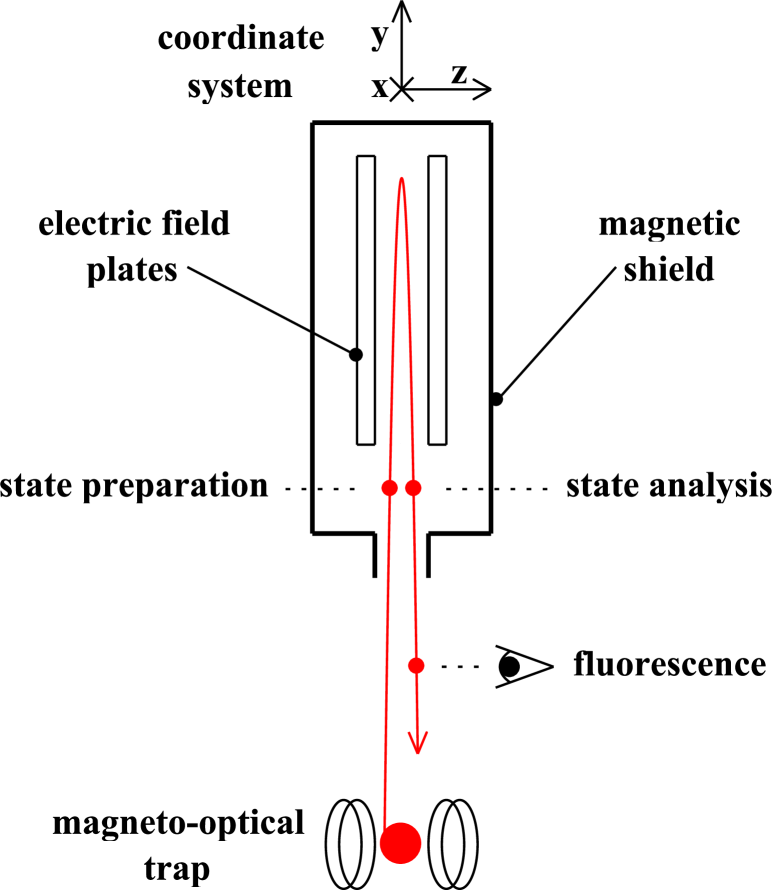
Figure 1: Schematic diagram of an experiment to measure an electron EDM using an atomic fountain. In the diagram the width of the parabolic trajectory has been greatly exaggerated. In first approximation, we assume that atoms rise and fall strictly along the $y$ axis, and that the applied electric field is strictly parallel to the $z$ axis. Atoms are exposed to lasers at the points on the trajectory marked by solid circles.

The system of optical pumping for state preparation uses the property that an atom illuminated with a laser tuned to an allowed transition with $\Delta F=0$ has a unique, known “dark” state from which excitation by the laser is forbidden. The dark state is a continuous function of the ellipticity of the laser polarization; for a linearly polarized laser with its axis of polarization parallel to the $z$ axis, the dark states is $\big{|}F,0\big{>}$, and for a laser propagating in the $z$ direction that is circularly polarized with positive helicity, the dark state is $\big{|}F,F\big{>}$. For conceptual simplicity, we mainly study initial states which are the coherent superpositions $(\big{|}F,M\big{>}\pm\big{|}F,-M\big{>})/\sqrt{2}$.

The system of optical pumping for state analysis (step $3$) is similar to that of state preparation (step $1$). An atom in any state of the upper, $F=I+1/2$ hyperfine level that is illuminated with a laser tuned to an allowed transition with $\Delta F=0$ will either end in the dark state of the laser or in some state of the lower hyperfine level. In the simple cases of a laser that is polarized parallel to the $z$ axis, or that propagates parallel to $z$ and is circularly polarized, we define the probability ${p}_{M}$ that an atom originally in the state $\big{|}F,M\big{>}$ ends in the dark state after multiple cycles of excitation to the $P_{j^{\prime}}$ state and spontaneous emission. For $\pi$ polarization, the dark state is $\big{|}F,0\big{>}$, because $(M=0)$–($M=0$) transitions are only allowed if the total angular momentum changes. The probabilities ${p}_{M}$ depend on the branching ratios for the various spontaneous transitions and can be found as simple fractions by solving the $2F+1$ equations for the evolution of the states of a given hyperfine level; the essential physics for the probabilities is illustrated for one particular transition in Fig. 2. In the calculation, the probability that an atom of nuclear spin $I$ in a $P$-state with quantum numbers $j^{\prime},F^{\prime},M^{\prime}$ undergoes a radiative transition to an $S_{1/2}$ state with quantum numbers $j,F,M$ is proportional to

$$(2j^{\prime}+1)^{2}\,(2F+1)\\ \left(\begin{array}[]{ccc}j&1&j^{\prime}\\ m&m^{\prime}-m&-m^{\prime}\end{array}\right)\,\left\{\begin{array}[]{ccc}F&1&F^{\prime}\\ j^{\prime}&I&j\end{array}\right\}\,,$$ (4)

where standard notation is used for the $3j$ and $6j$ symbols. One then sets up and solves the rate equations. In the rate equations, one may ignore the small frequency difference between the upper and lower hyperfine manifolds of the ground state $S_{1/2}\big{|}I\pm 1/2,M\big{>}$ indicated in Fig. 2, because the frequency difference to the upper state $P_{j^{\prime}}$ is much larger than the hyperfine splitting. The sets of values ${p}$ that are achievable for the case $F=4$ are listed in Tables 1 and 2; these turn out to be rational numbers. Values for $F=3$ and $F=5$ are found in Appendix B of Ref. WuMuJe2012app .

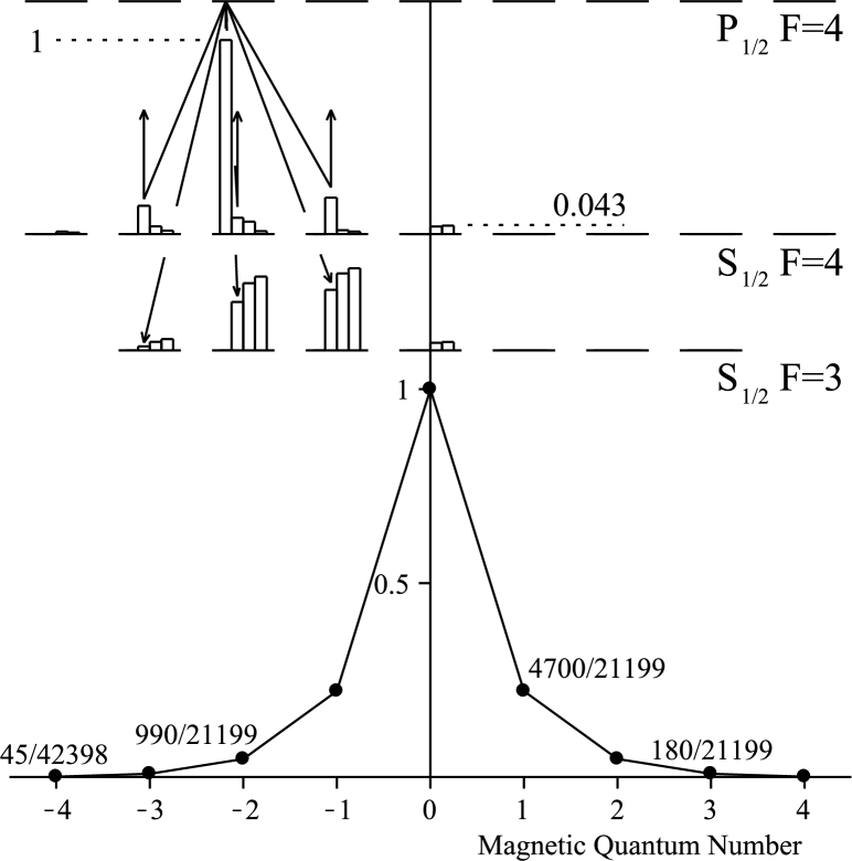
Figure 2: An atom, initially in the state $S_{1/2}\big{|}4,M\big{>}$, undergoes a large number of cycles of absorption of laser photons, followed by spontaneous emission. We define the probability ${p}_{M}$ to be the probability that an atom, illuminated with a $\pi$-polarized laser tuned to the transition $S_{1/2},\,F=4$ to $P_{1/2},\,F=4$, ends up in the dark $S_{1/2}\big{|}4,0\big{>}$ state instead of ending in some state in the $S_{1/2},\,F=3$ hyperfine level, after many cycles of absorption and spontaneous emission. In the upper half of the figure, the arrows show the pattern for the first spontaneous emission and re-excitation for an atom initially in state $S_{1/2}\big{|}4,-2\big{>}$, and the histograms show how the probability of being in any given level evolves after $0$, $1$, $2$, or $3$ spontaneous emissions. The probability of ending in the dark $S_{1/2}\big{|}4,0\big{>}$ state involves processes like $S_{1/2}\big{|}4,-2\big{>}\to P_{1/2}\big{|}4,-2\big{>}\to S_{1/2}\big{|}4,-1\big{>}\to P_{1/2}\big{|}4,-1\big{>}\to S_{1/2}\big{|}4,0\big{>}$ and similar. Values for $p_{M}$ are in the graph in the lower half of the figure, and correspond to those given in the second column of Table 1.

Table 1: For $I=7/2$, the probability $p_{M}$ that an atom, initially in the state $S_{1/2}\big{|}4,M\big{>}$, remains in the $F=4$ hyperfine level after being pumped with light tuned to the transition $S_{1/2},\,F=4\to P_{j^{\prime}},\,F^{\prime}$ that is linearly polarized with the axis of polarization parallel to $z$.

$P_{j^{\prime}}$	$P_{1/2}$	$P_{3/2}$	$P_{1/2}$	$P_{3/2}$
$F^{\prime}$	$4$	$4$	$3$	$3$
$S_{1/2}\big{|}4,M\big{>}$
$M=4$	$\frac{45}{42398}$	$\frac{151263}{23049298}$	$1$	$1$
$M=3$	$\frac{180}{21199}$	$\frac{345744}{11524649}$	$\frac{1792}{2585}$	$\frac{839216}{4101383}$
$M=2$	$\frac{990}{21199}$	$\frac{1205694}{11524649}$	$\frac{1092}{2585}$	$\frac{133868}{4101383}$
$M=1$	$\frac{4700}{21199}$	$\frac{3788344}{11524649}$	$\frac{112}{517}$	$\frac{15680}{4101383}$
$M=0$	$1$	$1$	$\frac{70}{517}$	$\frac{2450}{4101383}$
$M=-1$	$\frac{4700}{21199}$	$\frac{3788344}{11524649}$	$\frac{112}{517}$	$\frac{15680}{4101383}$
$M=-2$	$\frac{990}{21199}$	$\frac{1205694}{11524649}$	$\frac{1092}{2585}$	$\frac{133868}{4101383}$
$M=-3$	$\frac{180}{21199}$	$\frac{345744}{11524649}$	$\frac{1792}{2585}$	$\frac{839216}{4101383}$
$M=-4$	$\frac{45}{42398}$	$\frac{151263}{23049298}$	$1$	$1$

Table 2: For $I=7/2$ the probability $p_{M}$ that an atom initially in the state $S_{1/2}\big{|}4,4\big{>}$ remains in the $F=4$ hyperfine level after being pumped with light tuned to the transition $S_{1/2},\,F=4\to P_{j^{\prime}},\,F^{\prime}$, that propagates in the $z$ direction, and is circularly polarized with positive helicity.

$P_{j^{\prime}}$	$P_{1/2}$	$P_{3/2}$	$P_{1/2}$	$P_{3/2}$
$F^{\prime}$	$4$	$4$	$3$	$3$
$S_{1/2}\big{|}4,M\big{>}$
$M=4$	$1$	$1$	$1$	$1$
$M=3$	$\frac{4}{11}$	$\frac{28}{53}$	$1$	$1$
$M=2$	$\frac{80}{451}$	$\frac{3248}{10123}$	$\frac{35}{47}$	$\frac{35}{143}$
$M=1$	$\frac{1468}{17589}$	$\frac{352996}{1791771}$	$\frac{469}{705}$	$\frac{1141}{6721}$
$M=0$	$\frac{14774}{334191}$	$\frac{3868942}{30460107}$	$\frac{71}{141}$	$\frac{6965}{154583}$
$M=-1$	$\frac{7340}{334191}$	$\frac{2470972}{30460107}$	$\frac{1037}{2679}$	$\frac{186935}{10357061}$
$M=-2$	$\frac{155080}{13033449}$	$\frac{288122744}{5391438939}$	$\frac{7883}{29469}$	$\frac{1867985}{445353623}$
$M=-3$	$\frac{3196660}{534371409}$	$\frac{35621245604}{1029764837349}$	$\frac{4771}{29469}$	$\frac{15510145}{18259498543}$
$M=-4$	$\frac{18319475}{5878085499}$	$\frac{72657047561}{3210443316441}$	$\frac{688}{9823}$	$\frac{46289600}{529525457747}$

For the cases of linear and circular polarization, the probability that an atom, emerging from the atomic fountain in a general superposition of states $\sum A_{M}\big{|}F,M\big{>}$ for amplitudes $A_{M}$, ends in the dark state is simply $\sum|A_{M}|^{2}\,{p}_{M}$. Such a probability encodes information about the original atomic state in question and can be easily measured using fluorescent detection. Final read-out and normalization to the incoming flux of atoms proceeds as follows (step $4$): A cycling transition from the $S_{1/2}$ ground state with spin $F=I+1/2$ to the $P_{3/2}$ state with $F=I+3/2$ is rung and the photons counted; then a laser tuned to the transition from the lower hyperfine level of the ground state with $F=I-1/2$ to a $P$ state with $F=I+1/2$ puts all atoms into the $S$-state hyperfine level with $F=I+1/2$, and then the cycling transition $S_{1/2}\to P_{3/2}$ is fluoresced and the photons counted again; the ratio of the counts gives the probability.

An alkali atom of large nuclear charge would be indicated for our atomic fountain because relativistic effects enhance the EDM of such an atom compared to that of the free-electron by a large multiplicative factor $R$ (the “enhancement factor”). The theory of the enhancement factor is well-established, and has been used to set the EDM limits in Ref. PDG2010 . Computed values of the enhancement factors for Rb, Cs, and Fr are presented in Table 3. None of these computed factors have varied by more than $20\%$ from the earliest factors computed in 1966 (Ref. Sa1966 ), and an experiment to discover an EDM does not depend upon the error in the computed enhancement factor being small. Estimates of the size of limit that may be set by a francium fountain experiment operated at existing accelerator facilities may be found in Appendix A of Ref. WuMuJe2012app .

Table 3: Calculations of the enhancement factor $R$ for the ground state of heavy alkali atoms.

Alkali	R	Year	Reference
	$24$	1966	Sa1966
Rb	$24.6$	1985	JoGuIdSa1986
	$25.68$	1994	ShDaAn1994
	$25.74$	2008	NaSaDaMu2008
	$119$	1966	Sa1966
	$114.9$	1985	JoGuIdSa1986 ; JoGuIdSa1985
Cs	$114$	1990	MPOe1987 ; HaLiMP1990
	$120.54$	2008	NaSaDaMu2008
	$124$	2009	DzFl2009
	$1150.$	1966	Sa1966
Fr	$910$	1999	Byrnes1999
	$894.93$	2009	Mukherjee2009

A key part of any EDM measurement is controlling any systematic error that, like the effect of the EDM, reverses sign when the electric field is reversed. Such effects arise naturally in EDM experiments because in the rest frame of the atom, due to the atom’s nonzero velocity in the applied electric field, the atom sees (SI units) a magnetic field

$$\vec{B}_{\rm mot}=\frac{1}{c^{2}}\,\vec{v}\times\vec{E}\,,$$ (5)

which changes sign when $\vec{E}$ changes sign. The interaction of the atom’s magnetic moment with that motional magnetic field (Zeeman effect) then also changes sign when the direction of $\vec{E}$ is reversed. The rotation of the atom by this motional magnetic field, necessarily perpendicular to the electric field, cannot by itself generate a rotation about the electric-field axis. A priori, one would thus assume that the motional magnetic field does not mimic an EDM. However, in any practical apparatus, there will inevitably be present trace static magnetic fields which the atom will explore as it moves; the combinations of rotations about these fields and about the motional field are of concern.

In this paper, we present a complete categorization of all systematic errors that result from an atom in an atomic fountain being subjected to a constant electric field, the motional magnetic field, and trace magnetic fields which are static but may vary arbitrarily in all three spatial directions. The unitary operator that gives the time evolution of any superposition of magnetic sublevels $\big{|}F,M\big{>}$ is a complex matrix of dimension $(2F+1)\times(2F+1)$, where $F$ is the total spin of the hyperfine level. In an atomic fountain, the maximum atomic velocity $\sim 4\,{\rm m/s}$ is two orders of magnitude smaller than in previous atomic beam experiments ReCoScDM2002 , so the motional magnetic field also is reduced by two orders of magnitude. In an atomic fountain, atoms pass through each point in space twice, once rising and once falling; the resulting atom-by-atom reversal of the atomic velocity cancels some motional-field dependent systematics without a need for a second, antipropagating atomic beam. Let us briefly comment on the effect of a possible slight nonuniformity of the electric field, in which case the atomic trajectory may become more complicated because atoms in the level $S_{1/2},F=I+1/2$ are attracted into regions of strong electric field by the Stark shift. However, in our differential setup, we plan to measure the signal twice, with the sign of the electric field inverted, and in this case, even a more complicated trajectory is conserved and independent of the state of the atom, in the approximation that $\alpha_{F}^{S}\gg\alpha_{F}^{T}$ in Eq. (9).

Moreover, under the conditions of an atomic fountain, the shift of the magnetic sublevel $\big{|}F,M\big{>}$ due to the tensor Stark effect is now much greater than its shift due to the Zeeman effect. In a constant electric field, the unitary operator that gives the time evolution of any state can be computed as a series in reciprocal powers of a dimensionless parameter $\mu\sim 100$, which represents (roughly) the ratio of the shifts. The $(1/\mu)$-series therefore is rapidly convergent. We present this series as the sum of analytic integrals over the magnetic fields, times matrices of constants, for any of the total spins $F=3$, $4$, and $5$, and so for the spins of all the alkali atoms of experimental interest. We place special emphasis on the case $F=4$. A key result is that a properly constructed observable sensitive to an EDM will contain errors that are only even powers of $1/\mu$. Because contributions of order $1/\mu^{4}$ prove negligible in practice, any experiment only has to control the few terms of order $1/\mu^{2}$.

The coordinate system used to describe the atomic fountain is shown in Fig. 1. The atom remains on a single vertical axis, the $y$ axis. The direction of the electric field is horizontal and defines the $z$ axis. Therefore, the motional magnetic field is parallel to the $x$ axis. The effective Hamiltonian within a manifold of states of total spin $F$ is the sum of several pieces. The contribution of the electron EDM is

$$H_{\rm EDM}=R\,(-d_{{\mathrm{e}}})\,\vec{F}\cdot\vec{E}\,,$$ (6)

where $\vec{F}$ is the total angular momentum of the atom, $d_{{\mathrm{e}}}$ is the electron EDM, and $R$ is the enhancement factor. The contribution of the Zeeman effect is

$$H_{\rm Z}=\mu_{B}\,g_{F}\,\vec{F}\cdot\vec{B}\,,$$ (7)

where $\mu_{B}=\hbar|e|/(2m_{e}c)$ is the Bohr magneton and $g_{F}$ is the Landé $g$ factor for the manifold. The Stark effect contributes to each level $\big{|}F,M\big{>}$ the energy shift

$${\cal E}_{\rm S}=-\frac{1}{2}(\alpha_{0}+\alpha_{FM})\,E_{z}^{2}\,,$$ (8)

where $\alpha_{0}$ is the scalar polarizability (which is independent of $F$ and $M$) and $\alpha_{FM}$ is the tensor polarizability. The tensor polarizability splits DzEtAl2010 ; Sa1967Stark into the sum

$$\alpha_{FM}=\alpha^{S}_{F}+\frac{3M^{2}-F(F+1)}{F(2F-1)}\alpha^{T}_{F}\,,$$ (9)

where all dependence on the magnetic quantum number $M$ is explicit. The parts of $\alpha_{0}$ and of $\alpha_{FM}$ that are independent of $F_{z}$ contribute to a global shift of the whole hyperfine manifold and thus introduce no change in the atomic state other than a global phase. We may therefore drop them in solving for the time evolution of the atomic state. In doing so, we are well aware of the fact that, while the shifts do not affect the state, they still have a large effect on the motion of the atom. In general, the global shift of the hyperfine manifold implies that an atom accelerates as it enters an electric field. Furthermore, a parallel beam of atoms defocuses as it enters the electric field, because atoms are pulled towards the high-field region at the edges of the plates. Such defocusing can be compensated by a suitable set of electrostatic lenses KaLaGo2002 ; KaAmGo2005 ; Ka2011 .

Isolating the terms that are relevant for the quantum dynamics (mixing within the $F$-manifold), this gives an effective Hamiltonian

$$H_{\rm S}=A_{\rm S}\,E_{z}^{2}\,F_{z}^{2}\,,$$ (10)

where $A_{\rm S}$ is the constant

$$A_{\rm S}=-\frac{3\,\alpha_{F}^{T}}{2F(2F-1)}\,.$$ (11)

The total effective Hamiltonian $H_{\rm t}$ then is the sum of the tensor Stark term, the EDM term, and the Zeeman term,

$$H_{\rm t}=A_{\rm S}\,F_{z}^{2}\,E_{z}^{2}+\mu_{B}\,g_{F}\,\vec{F}\cdot\vec{B}-R\,d_{\rm e}\,F_{z}\,E_{z}\,.$$ (12)

Contributions to the effective Hamiltonian from the mixing of different hyperfine levels or from terms in the Stark effect of order $E_{z}^{4}$ (the hyperpolarizability FuRe1993 ) are negligible. A remark about the units in the Hamiltonian is necessary here. We have deliberately scaled the quantities in the Hamiltonians so that the total angular momentum $\vec{F}$ as well as the projection quantum number $F_{z}$ of a quantum state are dimensionless. To this end, we have absorbed $\hbar$ as the unit of the angular momentum into the respective moments and into the constant $A_{\rm S}$, using Eq. (3) for the EDM and using the usual definition of $\mu_{B}$.

The atoms enter the electric field and spend a time $T$ within it. In this paper, we do not consider effects due to a continuous rise of the electric field from zero, but model the rise as a step-function. In principle, the finite size of the transition region over which the electric field rises from zero to its full value will contribute to the time evolution operator in a rapidly convergent series in powers of the small time atoms spend in the transition region. The resulting systematics can be controlled by reducing static magnetic fields only in the transition region, whose vertical length will only be a few centimeters, without having to reduce the static magnetic fields everywhere in the whole fountain, whose vertical length will be about a meter. In order to simplify the calculations, we also introduce a dimensionless variable $t$ that runs from $-\tau$ to $\tau$, with $\tau=1/2$, while the usual time runs from zero to $T$. We then define a standard electric field strength $E_{S}$ by

$$E_{S}=\sqrt{\frac{\hbar}{T\,A_{\rm S}}}\,,$$ (13)

in order to render the Schrödinger equation dimensionless. (Note: to use this equation the units of $A_{S}$ have to be $J/(V/m)^{2}$.) The atom now evolves according to $H(t)\psi={\rm i}\,\partial\psi/\partial t$, where the Hamiltonian $H(t)$ is obtained from $H_{\rm t}$ given in Eq. (12) by an appropriate scaling,

$$H(t)=\epsilon_{z}^{2}(t)\,F_{z}^{2}+\vec{\beta}(t)\cdot\vec{F}+\sigma_{F}\,\epsilon_{z}(t)\,F_{z}\,.$$ (14)

Now $H(t)$ is dimensionless, and the (dimensionless) coefficients are

$$\epsilon_{z}(t)=\frac{E_{z}(t)}{E_{S}}\,,\ \,\,\,\,\vec{\beta}(t)=\frac{g_{F}\,\mu_{B}\,\vec{B}(t)}{A_{\rm S}\,E_{S}^{2}}\,,\ \,\,\,\,\sigma_{F}=-\frac{d_{\textrm{e}}\,R}{F\,A_{\rm S}\,E_{S}}\,.$$ (15)

The time-dependent Hamiltonian (14) is the basis of the entire derivation that follows. When the electric field is a constant in time, we define a time-independent parameter

$$\mu=\epsilon_{z}^{2}\,,$$ (16)

which for a typical experimental setup has values in the range $\mu\sim 100$.

II Time–Ordered Perturbation Theory

II.1 Hamiltonian and time evolution

Specializing the above general statements to an atom with a defined quantum number $F$, we now study the effective Hamiltonian in Eq. (14) for cesium (¹³³Cs), whose upper hyperfine level has $F=4$. As a simple model, consider the fountain of Fig. 1 with the atoms confined to the $y$ axis, with an electric field which might vary in magnitude but is always parallel to the $z$ axis, and a magnetic field which in the atom’s rest frame varies only slowly in time. We define $t$ as a dimensionless time variable. The ordinary (dimensional) time $\tilde{t}$, as measured by a clock, is related to $t$ as follows,

$$t=\left(\frac{\tilde{t}}{T}-\frac{1}{2}\right)\,.$$ (17)

The turning point of the atoms is at $\tilde{t}=\tfrac{1}{2}\,T$. The atoms enter the fountain at $\tilde{t}=0$, which corresponds to the scaled time variable $t=-{\textstyle{\frac{1}{2}}}$, and they leave the fountain at $t=+{\textstyle{\frac{1}{2}}}$. In the following, we employ the more general notation

$$-\tau\leq t\leq\tau\,,\qquad\qquad\tau={\textstyle{\frac{1}{2}}}\,.$$ (18)

This use of the symbol $\tau$ allows us to recognize time-symmetries in the calculation. For example, the motional magnetic field in the rest frame of an atom is odd around $t=0$ because the velocity changes sign there, while laboratory static magnetic fields are even in $t$.

The Hamiltonian (14) gives rise to a time evolution operator. Complete knowledge of this operator would allow us to propagate an initial state through the fountain and obtain the final state, which determines the observables. All effects which are either larger or about the size of the target sensitivity of $2\cdot 10^{-50}\,{\rm C\,m}$ have to be calculated if they could possibly mimic an electron EDM. At this stage, it is useful to recall that the traditional unit for the electron EDM is $e\,{\rm cm}$; the conversion to SI units is $1\,{\rm C\,m}=1.602\cdot 10^{-21}\,e\,{\rm cm}$. At the target sensitivity, the corresponding dimensionless parameter $\sigma_{F}$ in our Hamiltonian (14) has the value $\sigma_{F}=4\times 10^{-9}$ for cesium.

In the model calculation we consequently need to find all effects that would lead to an EDM-like signal of a magnitude greater than that of $\sigma_{F}$. Without the EDM term, the Hamiltonian reads as

$$H_{0}(t)=\epsilon_{z}^{2}(t)\,F_{z}^{2}+\vec{\beta}(t)\cdot\vec{F}\,.$$ (19)

The time-evolution governed by this Hamiltonian is characterized by the equation

$$H_{0}(t)\,U_{0}(t)={\mathrm{i}}\,\frac{\partial}{\partial t}U_{0}(t)\,,$$ (20)

with the initial condition $U(-\tau)=1$.

We first split this time evolution operator $U(t)$ into a diagonal part $V(t)$ and a remainder term $W(t)$. For $W(t)$, we define an equation of motion and write it as a time-ordered exponential $W(t)={\bm{T}}\exp(-{\mathrm{i}}\int_{-\tau}^{t}h(t^{\prime}){\mathrm{d}}t^{\prime})$, where $h(t)$ is defined in Eq. (27) below, and ${\bm{T}}$ denotes the time ordering (recall the symbol $T$ denotes instead the total time the atom spends in the fountain). Because $W(t)$ is expressed in terms of highly oscillatory integrals, for a constant magnetic field it is amenable to an expansion in the parameter $1/\mu$ where $\mu$ is defined in Eq. (16), with coefficients that depend on time-integrals over various components of the magnetic fields.

In the absence of magnetic fields in the $x$ and $y$ direction, the Hamiltonian $H_{0}(t)$ becomes

$$H^{\prime}_{0}(t)=\epsilon_{z}^{2}(t)\,F_{z}^{2}+\beta_{z}(t)\,F_{z}\,.$$ (21)

This Hamiltonian is diagonal in the hyperfine manifold, and its time-ordered exponential

$$V(t)={\bm{T}}\exp\left(-{\mathrm{i}}\int_{-\tau}^{t}H^{\prime}_{0}(t^{\prime}){\mathrm{d}}t^{\prime}\right)$$ (22)

is a diagonal $(2F+1)\times(2F+1)$ matrix acting on a $2F+1$ dimensional subspace of $M$ levels inside the manifold of a given total spin $F$, which can be written as

$$V(t)=\mathrm{diag}\!\left(\!\!\!\!\begin{matrix}\,\,\,\exp\Bigl{[}{-{\mathrm{i}}\!\int\limits_{-\tau}^{t}\!\left(F\beta_{z}(t^{\prime})+F^{2}\epsilon_{z}^{2}(t^{\prime})\right){\mathrm{d}}t^{\prime}}\Bigr{]}\qquad\qquad\;\\[8.61108pt] \,\exp\Bigl{[}{-{\mathrm{i}}\!\int\limits_{-\tau}^{t}\!\!\left((F\!-\!1)\beta_{z}(t^{\prime})\!+\!(F\!-\!1)^{2}\epsilon_{z}^{2}(t^{\prime})\right){\mathrm{d}}t^{\prime}}\!\Bigr{]}\\[4.30554pt] \vdots\\[4.30554pt] \!\!\exp\Bigl{[}{-{\mathrm{i}}\!\!\int\limits_{-\tau}^{t}\!\left((-F)\beta_{z}(t^{\prime})+(-F)^{2}\epsilon_{z}^{2}(t^{\prime})\right){\mathrm{d}}t^{\prime}}\Bigr{]}\end{matrix}\!\!\!\right)\,,$$ (23)

where $\mathrm{diag}$ denotes the diagonal matrix generated by the given matrix elements. It is now our aim to solve the full problem by writing the full time-evolution operator $U_{0}(t)$ as the product of the time-evolution operator for the diagonal part $V(t)$ and the remainder term $W(t)$, i.e.

$$U_{0}(t)=V(t)\,W(t)\,.$$ (24)

The required equation of motion for $W(t)$ can be found by using this product for $U(t)$ in Eq. (20), which gives

$$H_{0}(t)\,V(t)W(t)={\mathrm{i}}\,\frac{\partial}{\partial t}\left(V(t)W(t)\right)\,,\qquad H_{0}(t)V(t)W(t)-{\mathrm{i}}\frac{\partial V(t)}{\partial t}W(t)={\mathrm{i}}\,V(t)\frac{\partial W(t)}{\partial t}\,.$$ (25)

Multiplication with $V^{-1}(t)$ from the left leads to the equation

$${\mathrm{i}}\,\frac{\partial W(t)}{\partial t}=h(t)W(t)\,,\qquad h(t)=V^{-1}(t)H_{0}(t)V(t)-{\mathrm{i}}V^{-1}(t)\frac{\partial V(t)}{\partial t}\,.$$ (26)

The matrix representation of this new Hamiltonian $h(t)$ for general $F$ as a $(2F+1)\times(2F+1)$ matrix can be written in terms of the following, somewhat self-explanatory notation, where the $2F+1$ elements on the diagonal are written in the middle, the $2F$ entries of the sub-diagonal on the left, and the $2F$ entries of the super-diagonal on the right,

$$h(t)=\mathrm{diag}\begin{pmatrix}\ \ \ \ d_{F}f(t)\exp\left[-{\mathrm{i}}(2F-1)\int_{-\tau}^{t}\epsilon_{z}^{2}(t^{\prime})\,{\mathrm{d}}t^{\prime}\right]&0&\ \ \ \ d_{F}f^{*}(t)\exp\left[+{\mathrm{i}}(2F-1)\int_{-\tau}^{t}\epsilon_{z}^{2}(t^{\prime})\,{\mathrm{d}}t^{\prime}\right]\\[4.30554pt] \vskip 3.0pt plus 1.0pt minus 1.0pt\cr d_{F-1}f(t)\exp\left[-{\mathrm{i}}(2F-3)\int_{-\tau}^{t}\epsilon_{z}^{2}(t^{\prime})\,{\mathrm{d}}t^{\prime}\right]&0&d_{F-1}f^{*}(t)\exp\left[+{\mathrm{i}}(2F-3)\int_{-\tau}^{t}\epsilon_{z}^{2}(t^{\prime})\,{\mathrm{d}}t^{\prime}\right]\\[4.30554pt] \vdots&\vdots&\vdots\\ \ \ \ \ d_{F}f(t)\exp\left[+{\mathrm{i}}(2F-1)\int_{-\tau}^{t}\epsilon_{z}^{2}(t^{\prime})\,{\mathrm{d}}t^{\prime}\right]&0&\ \ \ \ d_{F}f^{*}(t)\exp\left[-{\mathrm{i}}(2F-1)\int_{-\tau}^{t}\epsilon_{z}^{2}(t^{\prime})\,{\mathrm{d}}t^{\prime}\right]\\ &0&\end{pmatrix}\,.$$ (27)

Here, $f(t)$ is a single complex function that contains all information about the magnetic fields in the atom’s rest frame,

$$f(t)=\big{(}\beta_{x}(t)+{\mathrm{i}}\,\beta_{y}(t)\big{)}\;\exp\left(-{\mathrm{i}}\int_{-\tau}^{t}\beta_{z}(t^{\prime})\,{\mathrm{d}}t^{\prime}\right)\,.$$ (28)

The coefficients $d_{F}$ need to be explained. They are defined as the corresponding entries (rational numbers and square roots of rational numbers) of the matrix representation of the $x$ component of the total angular momentum $\vec{F}$, which is $F_{x}=(F_{+}+F_{-})/2$. These entries are symmetric with respect to the transformation $M\to-M$, which is why we have been able to reduce the notation to the quantities $d_{M}$ with $M=1,\dots,F$ on the sub- and super-diagonals.

A central point of our proposed scheme is to require that the integral over the square of the cumulative scaled electric field strength seen by the atom along its path should be equal to an integer multiple $k_{\epsilon}$ of $\pi$,

$$\int_{-\tau}^{\tau}\epsilon_{z}^{2}(t)\,{\mathrm{d}}t\mathop{=}^{!}k_{\epsilon}\,\pi\,.$$ (29)

The adjustment to an integer value of $k_{\epsilon}$ has been used in a prototype experiment AmMuGo2007 ; Aminithesis2006 . According to Eq. (23), if the evolution of the hyperfine sublevels were exclusively given by the electric term (no motional or stray magnetic fields), then for $k_{\epsilon}$ even, the atomic wave function would return to its initial quantum state if the quantization condition (29) is fulfilled.

By measuring the temporally constant stray magnetic field seen by the atom, and by purposely applying a small additional magnetic field over the electric field plates, it is possible to also enforce a condition for the integral of the $z$ component of the magnetic field seen by the atom in the experiment,

$$\int_{-\tau}^{\tau}\beta_{z}(t)\,{\mathrm{d}}t\mathop{=}^{!}k_{\beta}\,\pi\,.$$ (30)

Here, it is the assumed that $k_{\beta}$ is tuned to be integer, and we note that $k_{\beta}=0$ is preferred; this value corresponds to small overall magnetic fields. Assuming that these adjustments can be achieved perfectly, the diagonal time-evolution operator $V(t)$ at the time $t=\tau$ when the atom leaves the fountain takes the simple form

$$V(\tau)=\mathrm{diag}\begin{pmatrix}(-1)^{F^{2}k_{\epsilon}}\;(-1)^{Fk_{\beta}}\\ \vskip 3.0pt plus 1.0pt minus 1.0pt\cr(-1)^{(F-1)^{2}k_{\epsilon}}\;(-1)^{(F-1)k_{\beta}}\\ \vdots\\ \vskip 3.0pt plus 1.0pt minus 1.0pt\cr\!\!\!\!\!(-1)^{(-F)^{2}k_{\epsilon}}\;(-1)^{-Fk_{\beta}}\end{pmatrix}\,,$$ (31)

which for even $k_{\epsilon}+k_{\beta}$ reduces to the unit matrix.

We express the remainder $W(t)$ of the time evolution operator as a time-ordered exponential in terms of a Dyson series. As we are only interested in its effect at the time $t=\tau$, when the atoms leave the fountain, we write

$$W(\tau)=1+\sum_{n=1}^{\infty}w_{n}\,.$$ (32)

The terms have the form

$$w_{n}=(-{\mathrm{i}})^{n}\!\!\int\limits_{-\tau}^{\tau}\int\limits_{-\tau}^{t_{1}}\cdots\int\limits_{-\tau}^{t_{n-1}}\!\!\!h(t_{1})\,h(t_{2})\!\ldots\!h(t_{n})\,{\mathrm{d}}t_{n}\ldots{\mathrm{d}}t_{2}\,{\mathrm{d}}t_{1}\,.$$ (33)

For the finite time interval $t\in[-\tau,\tau]$ considered in this work, the series for $W(t)$ is in fact convergent.

The basic idea of our theoretical analysis is as follows. The terms $w_{n}$ describe the deviation of the quantum dynamics from the idealized result (31) due to the magnetic field (28). Analytic estimates of the terms $w_{n}$ will allow us to gauge the magnitude and significance of individual EDM-mimicking signals with respect to our target sensitivity. An asymptotic expansion of the terms, based upon a separation of integrands into fast oscillating electric-field terms and slowly oscillating magnetic-field terms, leads to those estimates.

The asymptotic expansion is best illustrated by considering the first order term

$$w_{1}=(-{\mathrm{i}})\int_{-\tau}^{\tau}h(t_{1})\,{\mathrm{d}}t_{1}\,.$$ (34)

The nonzero entries of the $(2F+1)\times(2F+1)$ matrix $w_{1}$ are of the form

$$J=\int_{-\tau}^{\tau}f(t)\exp\left({\mathrm{i}}n\!\int_{-\tau}^{t}\!\!\!\epsilon_{z}^{2}(t^{\prime})\,{\mathrm{d}}t^{\prime}\right){\mathrm{d}}t\,,$$ (35)

where we use $n$ to represent the integers in the exponents in Eq. (27), and $f(t)$ is from Eq. (28). We envisage a situation where $|\epsilon_{z}(t)|^{2}$ is on the order of a hundred. The phase in the above integral is therefore highly oscillatory and the integral can be expressed in terms of an asymptotic expansion, as it is for example explained in Ref. BeOr1978 . This expansion is obtained by repeated integration by parts of Eq. (35) as

$$J= \biggl{[}\frac{{\mathrm{e}}^{{\mathrm{i}}n\int_{-\tau}^{t}\!\!\epsilon_{z}^{2}(t^{\prime})\,{\mathrm{d}}t^{\prime}}}{{\mathrm{i}}\,n\,\epsilon_{z}^{2}(t)}f(t)-\frac{{\mathrm{e}}^{{\mathrm{i}}n\int_{-\tau}^{t}\!\!\epsilon_{z}^{2}(t^{\prime})\,{\mathrm{d}}t^{\prime}}}{[{\mathrm{i}}\,n\,\epsilon_{z}^{2}(t)]^{2}}f^{\prime}(t)$$ (36)

$$+\frac{{\mathrm{e}}^{{\mathrm{i}}n\int_{-\tau}^{t}\!\!\epsilon_{z}^{2}(t^{\prime})\,{\mathrm{d}}t^{\prime}}}{[{\mathrm{i}}\,n\,\epsilon_{z}^{2}(t)]^{3}}\left(f^{\prime\prime}(t)-2f^{\prime}(t)\frac{\epsilon_{z}^{\prime}(t)}{\epsilon_{z}(t)}\right)\biggr{]}_{-\tau}^{\tau}\!\!\!+\ldots\,.$$

This equation expresses the time integral over an arbitrary integrand function $f(t)$ as a function of surface terms which need to be evaluated at the upper and lower limits of the time interval within the fountain. In our case, $f(t)$ is given by Eq. (28) and describes the dependence on the magnetic field seen by the atom as a function of the scaled time $t$. The expansion allows us to integrate out the fast oscillations due to the applied strong electric field and to concentrate, in the formulation of the quantum dynamics, on the dependence due to the residual magnetic fields (static and motional).

We can further simplify the expression for the expansion by noting that the exponential

$$\exp\left[\,{\mathrm{i}}\!\int_{-\tau}^{t}\epsilon_{z}^{2}(t^{\prime})\,{\mathrm{d}}t^{\prime}\right]\,,$$ (37)

evaluated at $t=-\tau$, assumes the value of unity. In all calculations where we employ this expansion, the integer $n$ in the exponentials in Eq. (27), which has one of the values $2F-1$, $2F-3,\ldots$, $-(2F-1)$, is odd. With the adjustment of the integral in Eq. (29), the exponential can be evaluated at $t=\tau$ to be

$$\exp\left[\,{\mathrm{i}}\,n\!\int_{-\tau}^{\tau}\epsilon_{z}^{2}(t^{\prime})\,{\mathrm{d}}t^{\prime}\right]={\mathrm{e}}^{{\mathrm{i}}nk_{\epsilon}\pi}=(-1)^{k_{\epsilon}}\,.$$ (38)

If in addition we assume the electric field to be constant, the formula for the asymptotic expansion of the integral $J$ then is written as

$$\begin{split}J=&\;\int_{-\tau}^{\tau}f(t)\exp\left[\,{\mathrm{i}}\,n\!\int_{-\tau}^{t}\!\!\!\epsilon_{z}^{2}(t^{\prime})\,{\mathrm{d}}t^{\prime}\right]{\mathrm{d}}t\\ =&-\frac{{\mathrm{i}}}{n\mu}\left((-1)^{k_{\epsilon}}f(\tau)-f(-\tau)\right)\\ &+\frac{1}{n^{2}\mu^{2}}\!\left((-1)^{k_{\epsilon}}f^{\prime}(\tau)-f^{\prime}(-\tau)\right)\\ &+\frac{{\mathrm{i}}}{n^{3}\mu^{3}}\left((-1)^{k_{\epsilon}}f^{\prime\prime}(\tau)-f^{\prime\prime}(-\tau)\right)+{\mathcal{O}}(\mu^{-4})\,.\end{split}$$ (39)

Such an expansion provides us with a tool to analyze the relative magnitude of the relevant physical effects. In our units used in this work the parameter $\mu$ for cesium is about $\mu\approx 120$, and for the envisaged sensitivity of an electron EDM the dimensionless EDM strength in Eq. (14) is $\sigma_{F}=4\times 10^{-9}$. Therefore, all EDM-mimicking effects of order $1/\mu^{4}\approx 4\cdot 10^{-9}$ have to be considered and eliminated in order to reach the target accuracy. In practice the actual coefficients of terms of order $1/\mu^{4}$ are small enough that their contribution is negligible, and for a suitable observable all effects of order $1/\mu^{n}$ for $n$ any odd integer can be proved to cancel, leaving only two terms of order $1/\mu^{2}$ to compute and to control. Using asymptotic expansions like that of Eq. (39) for the integrals appearing in $W(\tau)$, we are able to express the time-evolution operator

$$U_{0}(\tau)=V(\tau)\,W(\tau)={\bm{T}}\exp\left(-{\mathrm{i}}\int_{-\tau}^{\tau}H_{0}(t^{\prime}){\mathrm{d}}t^{\prime}\right)$$ (40)

when the electric field is constant in terms of an asymptotic series in inverse powers of $\mu$, which has the structure

$$U_{0}(\tau)=1$$ (41)

$$+\sum_{i=1}^{\infty}\!\frac{1}{\mu^{i}}\,\mathcal{T}_{i}\left(\left\{\int_{-\tau}^{\tau}\!\left[f^{(n)}(t)\right]^{m}\!\left[f^{*(k)}(\tau)\right]^{\ell}\!{\mathrm{d}}t\right\}_{\!n,m,k,\ell}\right)\,,$$

where the $\mathcal{T}_{i}$ are complex $(2F+1)\times(2F+1)$ dimensional coefficient functions that can be expressed in terms of integrals of the $n$th derivatives of the stray magnetic field function $f(t)$ or its complex conjugate $f^{*}(t)$, and in terms of powers thereof. This functional dependence is schematically indicated in Eq. (41) using the curly brackets and the multi-index $\{n,m,k,\ell\}$. We have carried out the calculation to fourth order in $1/\mu$, for $F=3$, $F=4$, and $F=5$. The individual expressions are too long to include in this paper, but the calculation is entirely based on the asymptotic expansion technique described herein.

The expansion of Eq. (41) has applicability beyond the case when the electric field is constant. Provided $\epsilon_{z}(t)$ is approximately constant on $[-\tau,\tau]$ there exists a transformation of the time variable that produces an equivalent problem where the electric field is exactly constant and where the unitary transformation is exactly of the form of Eq. (41), with a perturbed function $f$. As far as the cancellation of systematic effects in an electron EDM experiment, nothing has changed; only the numerical values of surviving systematics are perturbed.

Before we use this expansion to evaluate the specific terms of the time-evolution operator, we want to take the time and discuss the observable to be used in the experiment AmMuGo2007 ; Aminithesis2006 . The choice of the observable also identifies the EDM-mimicking effects.

II.2 Defining the observable

Without magnetic fields in the $x$ and $y$ direction, the only effect of the movement through the fountain for the atoms would be a rotation of the quantum states by a complex phase [see Eqs. (23) and (31)]. This follows because the phase adjustment of the magnetic field integral as well as the integral of the square of the electric field relevant to the Stark shift, sets the complex phase equal to a multiple of $\pi$. For $k_{\epsilon}+k_{\beta}$ even, the complex phase is a multiple of $2\pi$ and so the atoms are precisely rotated back into the initial state when they leave the fountain. The difference between the Hamiltonian with the EDM term given in Eq. (14) and the Hamiltonian without the EDM term given in Eq. (19) is that the presence of an EDM leads to a small additional rotation around the $z$ axis, and so the complex phase would no longer be zero (or equal to an integer multiple of $2\pi$). Therefore we need an observable that is sensitive to rotations about the $z$ axis.

In the case of ¹³³Cs, the valence electron is in the $6S_{1/2}$ state, so the atom can be in either of the two hyperfine levels $F=3$ or $F=4$. The atoms are prepared in a state $\left|4,M\right>$. After the atoms leave the fountain, the number of remaining atoms in the $F=4$ hyperfine level is measured and compared the total number of atoms. Some atoms can also transition into the $F=3$ hyperfine level of the $6S_{1/2}$ state.

Let us denote the state in the $F=I+1/2$ hyperfine level in which the atom is prepared before it enters the electric field as $\big{|}\Phi_{0}\big{>}$. After the atom exits the electric field, it is analyzed by optical pumping with a laser propagating in the $z$ direction and tuned to a $P$ state with spin $F^{\prime}=F$, where the laser is linearly polarized. We are interrogating quantum transitions with respect to quantum states whose quantization $x$ and $y$ axes are tilted by a rotation an angle $\theta$ with respect to the $z$ axis. The states on which we are projecting thus are the states $R_{z}(\theta)\big{|}F,M\big{>}$, where $R_{z}(\theta)$ is a suitable rotation operator. In this paper, we use the notation $R_{u}(\alpha)$ to indicate an operator that rotates a state on which it acts (active representation) about the axis denoted by $u$ and by an angle $\alpha$ that is positive if the rotation is in a positive sense about the axis $u$ as determined by the usual right-hand rule. Under these assumptions, we have $R_{z}(\theta)\big{|}F,M\big{>}=\exp(-{\mathrm{i}}M\,\theta)\,\big{|}F,M\big{>}$. The probability that the atom will be found in the dark state of the upper hyperfine level is our basic signal and is given by

$${\mathcal{S}}(\theta)=\sum_{M=-F}^{F}{p}_{M}\left|\left<FM\left|R_{z}(\theta)U(\tau)\;\right|\Phi_{0}\right>\right|^{2}.$$ (42)

where the constants ${p}_{M}$ can be chosen to be any of the sets in Tables 1 or Table 2. Here, $U(\tau)$ is the time-evolution operator of the full Hamiltonian (14),

$$U(\tau)={\bm{T}}\exp\left(-{\mathrm{i}}\int_{-\tau}^{\tau}H(t)\,{\mathrm{d}}t\right)\,.$$ (43)

A small rotation of the atomic states by an EDM can then be detected by taking two measurements at $\pm\theta$ and forming the difference. Thus, the observable $P(\theta)$ is given by the equation

$$\begin{split}P(\theta)&=\mathcal{S}(\theta)-\mathcal{S}(-\theta)\\ &=\!\!\!\sum_{M=-F}^{F}\!\!\!{p}_{M}\!\left(\left|\left<FM\left|R_{z}(+\theta)U(\tau)\right|\Phi_{0}\right>\right|^{2}\right.\\ &\qquad\quad\ \ \ \,\left.-\left|\left<FM\left|R_{z}(-\theta)U(\tau)\right|\Phi_{0}\right>\right|^{2}\right)\,,\end{split}$$ (44)

where because we are using a linearly polarized laser the probabilities ${p}_{M}$ have the symmetry ${p}_{M}={p}_{-M}$. This observable is measured again with the direction of the electric field reversed. The resulting difference is only sensitive to effects that, like that of an EDM, are odd under the reversal of the electric field direction.

The currently most promising alkali atoms for an actual experiment are cesium and francium. For cesium, the natural isotope ${}^{133}{\rm Cs}$ is suited best. It has nuclear spin $I=7/2$, and so the ground state $6S_{1/2}$ has the two hyperfine levels ${F=3}$ and ${F=4}$. The proposed detection scheme requires to use the energetically higher lying state $F=4$. For francium the enhancement factor $R$ is about nine times larger than in cesium, making this atom particularly attractive. The francium isotope ²²¹Fr, which has $I=5/2$, can be obtained from actinium sources and the dynamics of the $F=3$ hyperfine level would be investigated there. Due to a higher nuclear spin $I=9/2$, leading to a higher total angular momentum $F=5$ to be used for the dynamics, the francium isotope ²¹¹Fr, is currently the most promising atom to study. It can be obtained from accelerator sources, such as ISOLDE and TRIUMF, and its half-life of $3$ minutes is sufficiently long for a practical experiment. Yields of francium at existing and planned facilities (CERN ISOLDE and TRIUMF) and a discussion of the transfer mechanism from the beam to the magneto-optical trap can be found in Refs. ISOLDE_fr ; TRIUMF_fr ; TRIUMF_plan ; PROJECTX ; AuGoOrSp2003 ; MeEtAl2004 .

In the calculation of $P(\theta)$, it is possible to perform a basis transformation which leads to a number of simplifications. We define as our new basis states the following superpositions of the sublevels $\pm M$, which are obtained from the original basis states $|FM\rangle$ by a rotation about an angle $\pi/2$ around the $y$ axis,

$$|s_{M}\rangle =\frac{1}{\sqrt{2}}\,R_{y}(\pi/2)\left(\left|FM\right>+\left|F\;-M\right>\right)\,,$$ (45)

$$|a_{M}\rangle =\frac{1}{\sqrt{2}}\,R_{y}(\pi/2)\left(\left|FM\right>-\left|F\;-M\right>\right)\,.$$ (46)

Here $R_{y}(\pi/2)$ is the corresponding rotation operator, and we index the new states by their dependence on $M$ and suppress the subscript $F$. These new states may also be used for the projections carried out in the calculation of $P(\theta)$.

The new states have useful symmetries under two transformations. Let us define the matrix $B$, which has the entries

$$B_{ij}=(-1)^{i+1}\,\delta_{i,j}\,,$$ (47)

where the indices run from $1$ to $2F+1$. This matrix is trivially generalized to $F=3$, $4$, and $5$: the $B$ matrix is a diagonal $(2F+1)\times(2F+1)$ matrix where the first matrix elements on the diagonal run $+1,-1,+1,\dots$. The states $|s_{M}\rangle$ are eigenstates of $B$ with eigenvalue $+1$, while the states $|a_{M}\rangle$ are eigenstates of $B$ with eigenvalue $-1$.

The new states also have a symmetry under exchange of magnetic quantum numbers from $M$ to $-M$. This exchange can be described by transformation by a second $(2F+1)\times(2F+1)$ matrix $S$ that has entries

$$S_{ij}=\delta_{i,(2F+1)-j}\,.$$ (48)

Both $|s_{M}\rangle$ and $|a_{M}\rangle$ are eigenstates of $S$ with eigenvalues $(-1)^{F+M}$.

In terms of these new states, and in the case where $p_{M}=p_{-M}$, we can rewrite $P(\theta)$ as

$$\begin{split}P(\theta)=&\sum_{M=0}^{F}{p}_{M}\left(\left|\left<s_{M}\left|R_{z}(\theta)U(\tau)\right|\Phi_{0}\right>\right|^{2}\right.\\ &\qquad\quad\left.-\left|\left<s_{M}\left|R_{z}^{\dagger}(\theta)U(\tau)\right|\Phi_{0}\right>\right|^{2}\right)\\ +{}&\sum_{M=1}^{F}{p}_{M}\left(\left|\left<a_{M}\left|R_{z}(\theta)U(\tau)\right|\Phi_{0}\right>\right|^{2}\right.\\ &\qquad\quad\left.-\left|\left<a_{M}\left|R_{z}^{\dagger}(\theta)U(\tau)\right|\Phi_{0}\right>\right|^{2}\right)\,,\end{split}$$ (49)

where we have used the fact that $R_{z}(-\theta)=R_{z}^{\dagger}(\theta)$.

The great utility of the inversion symmetry becomes clear in the next step, as it allows us to express the difference of the measurements at $\pm\theta$ instead in a simpler, product form [see Eq. (51) below]. We define the “even” part of a matrix $A$ as

$$O_{+}(A)={\textstyle{\frac{1}{2}}}(A+SAS)\,,$$

which is even under conjugation with $S$,

$$SO_{+}(A)S={\textstyle{\frac{1}{2}}}S(A+SAS)S=O_{+}(A)\,,$$

because $SS=1$. The “odd” part

$$O_{-}(A)={\textstyle{\frac{1}{2}}}(A-SAS)\,$$

is odd under conjugation with $S$,

$$SO_{-}(A)S={\textstyle{\frac{1}{2}}}S(A-SAS)S=-O_{-}(A)\,.$$

Due to the identity [we use $R_{z}\equiv R_{z}(\theta)$]

$$\bigl{|}\langle\psi_{2}\left|R_{z}A\bigr{|}\psi_{1}\rangle\right|^{2}-\left|\langle\psi_{2}\left|R_{z}^{\dagger}A\right|\psi_{1}\rangle\right|^{2}=-4\mathrm{Re}\langle\psi_{1}\left|O_{-}(A^{\dagger})R_{z}\right|\psi_{2}\rangle\langle\psi_{2}\left|R_{z}^{\dagger}O_{+}(A)\right|\psi_{1}\rangle\,,$$ (50)

we have the following expression for $P(\theta)$,

$$\begin{split}P(\theta)=&-4\,\mathrm{Re}\biggl{[}\sum_{M=0}^{F}{p}_{M}\left<\Phi_{0}\left|O_{-}(U^{\dagger}(\tau))\right|R_{z}^{\dagger}(\theta)s_{M}\right>\left<R_{z}(\theta)s_{M}\left|O_{+}(U(\tau))\right|\Phi_{0}\right>\biggr{]}\\ &-4\,\mathrm{Re}\biggl{[}\sum_{M=1}^{F}{p}_{M}\left<\Phi_{0}\left|O_{-}(U^{\dagger}(\tau))\right|R_{z}^{\dagger}(\theta)a_{M}\right>\left<R_{z}(\theta)a_{M}\left|O_{+}(U(\tau))\right|\Phi_{0}\right>\biggr{]}\,.\end{split}$$ (51)

This is an improvement on Eq. (49) in that we have expressed the difference between the measurements at $\pm\theta$ as the real part of a product: of the part of the time-evolution operator evaluated at $t=\tau$ that is even under conjugation with $S$; and a part which is odd under conjugation with $S$. In addition, we have separated the projection onto intermediate states that are even and odd under conjugation with $B$, namely $|s_{M}\rangle$ and $|a_{M}\rangle$, respectively.

For $k_{\epsilon}+k_{\beta}$ even, we can use $W(\tau)$ instead of $U(\tau)$ because $V(\tau)$ is the identity matrix. For $k_{\epsilon}+k_{\beta}$ odd, the effect of $V(\tau)$ is a minus sign for each of the matrix elements containing $a_{M}$ for $F=4$, which as we will see later do not contribute to an EDM or EDM-mimicking signal. We are therefore safe to just use $W(\tau)$ instead $U(\tau)$. Using Eq. (32), $P(\theta)$ can now be rewritten as

$$\begin{split}-\frac{P(\theta)}{4}=\mathrm{Re}\biggl{[}\,&\sum_{M=0}^{F}\!\,{p}_{M}\biggl{<}\!\Phi_{0}\biggl{|}O_{-}\biggl{(}\,\sum_{n=1}^{\infty}w_{n}\biggr{)}^{\!\!\dagger}\biggr{|}R_{z}^{\dagger}(\theta)s_{M}\!\!\biggr{>}\biggl{<}R_{z}(\theta)s_{M}\biggl{|}O_{+}\biggl{(}1+\sum_{n=1}^{\infty}w_{n}\biggr{)}\biggr{|}\Phi_{0}\biggr{>}\\[8.61108pt] +{}&\sum_{M=1}^{F}{p}_{M}\biggl{<}\!\Phi_{0}\biggl{|}O_{-}\biggl{(}\sum_{n}w_{n}\biggr{)}^{\!\!\dagger}\biggr{|}R_{z}^{\dagger}(\theta)a_{M}\!\!\biggr{>}\biggl{<}R_{z}(\theta)a_{M}\biggl{|}O_{+}\biggl{(}1+\sum_{n}w_{n}\biggr{)}\biggr{|}\Phi_{0}\biggr{>}\,\biggr{]}\,.\end{split}$$ (52)

Here, use is made of the fact that $O_{-}(1)=0$. The observable now being known, we can employ the asymptotic expansion to determine the matrices $O_{\pm}(w_{n})$ which describe the time-evolution of the atoms through the fountain to identify EDM-mimicking effects. We begin by determining the terms in the first order of the Dyson series.

II.3 First term of the expansion of $\bm{W}$

We continue to use the Hamiltonian $h(t)$, which does not contain a possible EDM, in order to isolate all effects that could mimic the presence of an EDM. We obtain the unitary transformation accurate to order $1/\mu^{2}$, for which as we shall see it is necessary to consider some terms at fourth order in time-ordered perturbation theory. Knowing the terms in the unitary transformation to order $1/\mu^{2}$ proves to be sufficient to describe all EDM-mimicking effects in a suitable observable with error of order $1/\mu^{4}$. The calculational scheme for our observable $P(\theta)$ implies that we have to determine the $S$-even part of the matrix $w_{1}$, denoted as $O_{+}(w_{1})$, and the $S$-odd part, denoted as $O_{-}(w_{1})$, separately. We present these characteristic calculations in some detail and start by giving the matrix for $O_{+}(w_{1})$, which for general $F$ has the form

$$O_{+}(w_{1})\!=\!\mathrm{diag}\!\begin{pmatrix}\ \ \ \ \,-{\mathrm{i}}d_{F}\!\!\int\limits_{-\tau}^{\tau}\!\!\mathrm{Re}\!\left[f(t)\right]\exp\Bigl{[}-{\mathrm{i}}(2F\!-\!1)\!\!\int\limits_{-\tau}^{t}\!\!\epsilon_{z}^{2}(t^{\prime}){\mathrm{d}}t^{\prime}\Bigr{]}{\mathrm{d}}t&0&\ \ \ \ -{\mathrm{i}}d_{F}\!\!\int\limits_{-\tau}^{\tau}\!\!\mathrm{Re}\!\left[f(t)\right]\exp\Bigl{[}+{\mathrm{i}}(2F\!-\!1)\!\!\int\limits_{-\tau}^{t}\!\!\epsilon_{z}^{2}(t^{\prime}){\mathrm{d}}t^{\prime}\Bigr{]}{\mathrm{d}}t\\ \vskip 3.0pt plus 1.0pt minus 1.0pt\cr-{\mathrm{i}}d_{F-1}\!\!\int\limits_{-\tau}^{\tau}\!\!\mathrm{Re}\!\left[f(t)\right]\exp\Bigl{[}-{\mathrm{i}}(2F\!-\!3)\!\!\int\limits_{-\tau}^{t}\!\!\epsilon_{z}^{2}(t^{\prime}){\mathrm{d}}t^{\prime}\Bigr{]}{\mathrm{d}}t&0&-{\mathrm{i}}d_{F-1}\!\!\int\limits_{-\tau}^{\tau}\!\!\mathrm{Re}\!\left[f(t)\right]\exp\Bigl{[}+{\mathrm{i}}(2F\!-\!3)\!\!\int\limits_{-\tau}^{t}\!\!\epsilon_{z}^{2}(t^{\prime}){\mathrm{d}}t^{\prime}\Bigr{]}{\mathrm{d}}t\\ \vdots&\vdots&\vdots\\ \ \ \ \ \,-{\mathrm{i}}d_{F}\!\!\int\limits_{-\tau}^{\tau}\!\!\mathrm{Re}\!\left[f(t)\right]\exp\Bigl{[}+{\mathrm{i}}(2F\!-\!1)\!\!\int\limits_{-\tau}^{t}\!\!\epsilon_{z}^{2}(t^{\prime}){\mathrm{d}}t^{\prime}\Bigr{]}{\mathrm{d}}t&0&\ \ \ \ \,-{\mathrm{i}}d_{F}\!\!\int\limits_{-\tau}^{\tau}\!\!\mathrm{Re}\!\left[f(t)\right]\exp\Bigl{[}-{\mathrm{i}}(2F\!-\!1)\!\!\int\limits_{-\tau}^{t}\!\!\epsilon_{z}^{2}(t^{\prime}){\mathrm{d}}t^{\prime}\Bigr{]}{\mathrm{d}}t\\ &0&\end{pmatrix}\,,$$ (53)

where the $d_{F}$ are the corresponding entries in the matrix $F_{x}$. A simple calculation reveals that $Sw_{1}S$ can be obtained out of $w_{1}$ by exchanging $f(t)$ and $f^{*}(t)$. The entries of $O_{+}(w_{1})$ are thus $f(t)+f^{*}(t)$, which is twice the real part of $f(t)$.

Similarly, in $O_{-}$, the difference of the function $f(t)$ from Eq. (28) and its complex conjugate gives the imaginary part of $f(t)$. There is an additional minus sign for the super diagonal because of the different order of $f$ and $f^{*}$. As a result of the calculation, $O_{-}(w_{1})$ is found to be

$$O_{-}(w_{1})=\mathrm{diag}\begin{pmatrix}\;\;\;d_{F}\!\!\int\limits_{-\tau}^{\tau}\!\mathrm{Im}\!\left[f(t)\right]\exp\Bigl{[}-{\mathrm{i}}(2F\!-\!1)\!\!\int\limits_{-\tau}^{t}\!\!\epsilon_{z}^{2}(t^{\prime}){\mathrm{d}}t^{\prime}\Bigr{]}{\mathrm{d}}t&\;0&\;\;\;\,-d_{F}\!\!\int\limits_{-\tau}^{\tau}\!\mathrm{Im}\!\left[f(t)\right]\exp\Bigl{[}+{\mathrm{i}}(2F\!-\!1)\!\!\int\limits_{-\tau}^{t}\!\epsilon_{z}^{2}(t^{\prime}){\mathrm{d}}t^{\prime}\Bigr{]}{\mathrm{d}}t\\ \vskip 3.0pt plus 1.0pt minus 1.0pt\cr d_{F-1}\!\!\int\limits_{-\tau}^{\tau}\!\mathrm{Im}\!\left[f(t)\right]\exp\Bigl{[}-{\mathrm{i}}(2F\!-\!3)\!\!\int\limits_{-\tau}^{t}\!\epsilon_{z}^{2}(t^{\prime}){\mathrm{d}}t^{\prime}\Bigr{]}{\mathrm{d}}t&\;0&-d_{F-1}\!\!\int\limits_{-\tau}^{\tau}\!\mathrm{Im}\!\left[f(t)\right]\exp\Bigl{[}+{\mathrm{i}}(2F\!-\!3)\!\!\int\limits_{-\tau}^{t}\!\epsilon_{z}^{2}(t^{\prime}){\mathrm{d}}t^{\prime}\Bigr{]}{\mathrm{d}}t\\ \vdots&\;\vdots&\vdots\\ \;\;\;\;d_{F}\!\!\int\limits_{-\tau}^{\tau}\!\mathrm{Im}\!\left[f(t)\right]\exp\Bigl{[}+{\mathrm{i}}(2F\!-\!1)\!\!\int\limits_{-\tau}^{t}\!\epsilon_{z}^{2}(t^{\prime}){\mathrm{d}}t^{\prime}\Bigr{]}{\mathrm{d}}t&\;0&\;\;\;\,-d_{F}\!\!\int\limits_{-\tau}^{\tau}\!\mathrm{Im}\!\left[f(t)\right]\exp\Bigl{[}-{\mathrm{i}}(2F\!-\!1)\!\!\int\limits_{-\tau}^{t}\!\epsilon_{z}^{2}(t^{\prime}){\mathrm{d}}t^{\prime}\Bigr{]}{\mathrm{d}}t\\ &\;0&\end{pmatrix}\,.$$ (54)

If $n=-(2F-1)$, $\dots$, $2F-1$ denotes the prefactor in the exponentials of the matrix elements of $O_{+}(w_{1})$, then when $\epsilon_{z}$ is constant we find by asymptotic expansion with error $\mathcal{O}(\mu^{-3})$ we have

$$\begin{split}\left[O_{+}(w_{1})\right]_{n}=\frac{d_{j}}{n}\frac{1}{\mu}&\left[\mathrm{Re}[f(-\tau)]-\mathrm{Re}[f(\tau)](-1)^{k_{\epsilon}}\right]\\ +{\mathrm{i}}\frac{d_{j}}{n^{2}}\frac{1}{\mu^{2}}&\left[\mathrm{Re}[f^{\prime}(-\tau)]-\mathrm{Re}[f^{\prime}(\tau)]\,(-1)^{k_{\epsilon}}\right]\,.\end{split}$$ (55)

The function $f$ is given by

$$f(t)=\left[\beta_{x}(t)+{\mathrm{i}}\,\beta_{y}(t)\right]e^{-{\mathrm{i}}B(t)}\,,$$ (56)

with

$$B(t)=\int_{-\tau}^{t}\beta_{z}(t^{\prime})\,{\mathrm{d}}t^{\prime}\,.$$ (57)

We can simplify results by using the time-symmetry of fields in an atomic fountain. Because the atom is assumed to rise and fall along the $y$ axis, it passes through the same static magnetic fields when both rising and falling. In the rest frame of the atom the magnetic fields applied this way are time-even, i.e., even around the time $t=0$. Similarly the electric field applied in atom’s rest frame, due to the atoms motion through a static electric field that we have assumed is parallel to the $z$ axis, is time-even. The motional magnetic field applied in the atom’s rest frame, which arises due to the Lorentz transformation of the electric field and in our geometry is always parallel to the $x$ axis, is time-odd around ${t=0}$ because the atomic velocity changes sign when the atom falls while the direction of the electric field does not.

We can split the magnetic field along the $x$ axis, $\beta_{x}(t)$, into its static and time-even part $x_{e}(t)$ and its motional magnetic and time-odd part $x_{o}(t)$. Thus we have the following facts:

• $x_{o}(t)\equiv\beta_{x}({\mathrm{motion}};t)$    is time-odd,

• $x_{e}(t)\equiv\beta_{x}({\mathrm{static}};t)$    is time-even,

• $y_{e}(t)\equiv\beta_{y}({\mathrm{static}};t)$    is time-even,

• $\epsilon_{z}(t)$ is time-even around $t=0$,

• $z_{e}(t)\equiv\beta_{z}({\mathrm{static}};t)$ is time-even,
  and in addition $B(\tau)=\int_{-\tau}^{\tau}\beta_{z}(t^{\prime})\,dt^{\prime}=k_{\beta}\pi$.

Again specializing to the case of a constant electric field $\epsilon_{z}$, to order $1/\mu$ we find

$$\mathrm{Re}[f(-\tau)]-\mathrm{Re}[f(\tau)](-1)^{k_{\epsilon}}=\mathrm{Re}\left[\beta_{x}(-\tau)+{\mathrm{i}}\beta_{y}(-\tau)\right]$$

$$\qquad-(-1)^{{k_{\epsilon}}+k_{\beta}}\;\mathrm{Re}\left[\beta_{x}(\tau)+{\mathrm{i}}\beta_{y}(\tau)\right]$$ (58)

$$\qquad=\beta_{x}(-\tau)-(-1)^{{k_{\epsilon}}+k_{\beta}}\beta_{x}(\tau)\,.$$

Separating the magnetic field in the $x$ direction into its static and motional part and employing the time-symmetries in the ideal fountain, we obtain the result

$$\;\beta_{x}(-\tau)-(-1)^{k_{\epsilon}+k_{\beta}}\beta_{x}(\tau)$$

$$\qquad=x_{e}(-\tau)+x_{o}(-\tau)-(-1)^{k_{\epsilon}+k_{\beta}}\left[x_{e}(\tau)+x_{o}(\tau)\right]$$

$$\qquad=\left\{\begin{array}[]{ll}2x_{o}(-\tau)&\textrm{for}\;k_{\epsilon}+k_{\beta}\;\textrm{even}\,,\\[4.30554pt] 2x_{e}(-\tau)&\textrm{for}\;k_{\epsilon}+k_{\beta}\;\textrm{odd}\,.\end{array}\right.$$ (61)

To get the contribution of order $1/\mu^{2}$, we need the derivative

$$\begin{split}f^{\prime}(t)&=\frac{{\mathrm{d}}}{{\mathrm{d}}t}\left[\beta_{x}(t)+{\mathrm{i}}\beta_{y}(t)\right]e^{-{\mathrm{i}}B(t)}\\ &=\bigl{[}\beta_{x}^{\prime}(t)+{\mathrm{i}}\beta_{y}^{\prime}(t)\bigr{]}e^{-{\mathrm{i}}B(t)}\\ &\qquad-{\mathrm{i}}\beta_{z}(t)\bigl{[}\beta_{x}(t)+{\mathrm{i}}\beta_{y}(t)\bigr{]}e^{-{\mathrm{i}}B(t)}\,,\end{split}$$ (62)

which allows us to obtain

$$\begin{split}&\;\mathrm{Re}[f^{\prime}(-\tau)]-\mathrm{Re}[f^{\prime}(\tau)](-1)^{k_{\epsilon}}=y_{e}(-\tau)z_{e}(-\tau)\\ &\qquad-(-1)^{k_{\epsilon}+k_{\beta}}y_{e}(-\tau)z_{e}(-\tau)\\ &\qquad+x_{e}^{\prime}(-\tau)+x_{o}^{\prime}(-\tau)-(-1)^{k_{\epsilon}+k_{\beta}}x_{e}^{\prime}(\tau)x_{o}^{\prime}(\tau)\,.\end{split}$$ (63)

Because the time derivative an odd function of time is even, and the derivative of an even function is odd, we get

$$y_{e}(-\tau)z_{e}(-\tau)-(-1)^{k_{\epsilon}+k_{\beta}}y_{e}(-\tau)z_{e}(-\tau)$$

$$\quad+x_{e}^{\prime}(-\tau)+x_{o}^{\prime}(-\tau)-(-1)^{k_{\epsilon}+k_{\beta}}x_{e}^{\prime}(\tau)x_{o}^{\prime}(\tau)$$ (64)

$$\qquad=\left\{\begin{array}[]{ll}2x_{e}^{\prime}(-\tau)&\textrm{for}\;k_{\epsilon}+k_{\beta}\;\textrm{even}\,,\\[4.30554pt] 2y_{e}(-\tau)z_{e}(-\tau)+2x_{o}^{\prime}(-\tau)&\textrm{for}\;k_{\epsilon}+k_{\beta}\;\textrm{odd}\,.\end{array}\right.$$ (67)

We also define a standard form for the expansion of the matrices $O_{+}(w_{n})$, which takes the form

$$O_{+}(w_{n})=\sum_{k=k_{0}}^{\infty}\frac{{\mathrm{i}}^{n+k}}{\mu^{k}}\sum_{j}\mathcal{N}_{n,k}^{(j)}(F)\,\mathcal{G}_{n,k}^{(j)}(\vec{\beta}(t))\,,$$ (68)

where the $\mathcal{N}^{(j)}_{n,k}$ are matrices of dimension $(2F+1)\times(2F+1)$ whose entries are real, field-independent constants that depend on $F$. The expressions $\mathcal{G}^{(j)}_{n,k}$ are also real and can have a rather complicated dependence on the magnetic field $\vec{\beta}(t)$, as well as integrals, derivatives and of powers thereof, but are independent of $F$. The sum over $j$ is introduced to effect a natural separation of the terms of a given order in $n$ and $k$ according to specific symmetry properties of the field-dependent functions $\mathcal{G}^{(j)}_{n,k}$, as explained below.

In first order in $n$, where the subscript $n$ denotes the expansion order for the time-ordered perturbation theory, only a single term with $j=1$ is required, and we can suppress the superscript $j$ in our notation; the sum over $j$ becomes necessary only for the second and higher orders ($n=2,3,\dots$). Low-order terms in $n$ will nonetheless contribute to high orders in $1/\mu$. Corresponding to each $n$ is however a lowest-order nonvanishing contribution in $1/\mu$. While one’s initial guess would be that the sum over the inverse powers of $1/\mu$ starts at $k=n$, in fact this sum starts at the value $k_{0}$ defined by

$$k_{0}\equiv k_{0}(n)=\left\{\begin{array}[]{cl}{n}/{2}&\textrm{for}\;n\;\textrm{even,}\\[4.30554pt] ({n+1})/{2}&\textrm{for}\;n\;\textrm{odd}\,,\end{array}\right.$$ (69)

or in an alternative notation as the ceiling of $n/2$ (i.e., the smallest integer larger than or equal to $n/2$). This more complicated rule arises from the cancellations among the various exponential factors in various integrands, as explained in more detail below.

For $O_{-}(w_{n})$, we define an analogous series by

$$O_{-}(w_{n})=\sum_{k=k_{0}}^{\infty}\frac{{\mathrm{i}}^{n+k+1}}{\mu^{k}}\sum_{j}\mathcal{M}^{(j)}_{n,k}(F)\,\mathcal{B}^{(j)}_{n,k}(\vec{\beta}(t))\,,$$ (70)

where we now use $\mathcal{M}$ to denote the respective matrices of real field-independent constants; $\mathcal{B}$ for the respective magnetic-field dependent, real expressions; and where $k_{0}$ is as defined in Eq. (69). The matrices $\mathcal{M}$ and $\mathcal{N}$ as well as the expressions $\mathcal{G}$ and $\mathcal{B}$ can be shown to be real to all orders. Because the only imaginary factors in Eqs. (68) and (70) are the explicit powers of ${\mathrm{i}}$, it is straightforward later to take the real part of the observable $P(\theta)$.

Suppressing for simplicity of notation the magnetic field dependence of $\mathcal{G}^{(j)}_{n,k}$, the leading contributions to $O_{+}(w_{1})$ can be written

$$\begin{split}O_{+}(w_{1})&=-\frac{1}{\mu}\mathcal{N}_{1,1}(F)\;\mathcal{G}_{1,1}\\ &\qquad-\frac{{\mathrm{i}}}{\mu^{2}}\mathcal{N}_{1,2}(F)\;\mathcal{G}_{1,2}+\mathcal{O}(\mu^{-3})\,,\end{split}$$ (71)

with the functions

$$\mathcal{G}_{1,1}=\left\{\begin{array}[]{ll}2x_{o}(-\tau)&\textrm{for}\;k_{\epsilon}+k_{\beta}\;\textrm{even},\\[4.30554pt] 2x_{e}(-\tau)&\textrm{for}\;k_{\epsilon}+k_{\beta}\;\textrm{odd},\end{array}\right.$$ (72)

and

$$\mathcal{G}_{1,2}\!=\!\left\{\begin{array}[]{ll}\!\!2x_{e}^{\prime}(-\tau)&\textrm{for}\;k_{\epsilon}\!\!+\!k_{\beta}\,\textrm{even},\\[4.30554pt] \!\!2y_{e}(-\tau)z_{e}(-\tau)\!+\!2x_{o}^{\prime}(-\tau)&\textrm{for}\;k_{\epsilon}\!\!+\!k_{\beta}\,\textrm{odd}.\end{array}\right.$$ (73)

The coefficient matrices $\mathcal{N}$ for cesium with $F=4$ have the form

$$\mathcal{N}_{1,1}(4)=-\mathrm{diag}\begin{pmatrix}-{\sqrt{2}}/{7}&0&\phantom{-}{\sqrt{2}}/{7}\\ -{\sqrt{14}}/{10}&0&\phantom{-}{\sqrt{14}}/{10}\\ -{\sqrt{2}}/{2}&0&\phantom{-}{\sqrt{2}}/{2}\\ -\sqrt{5}&0&\phantom{-}\sqrt{5}\\ \phantom{-}\sqrt{5}&0&-\sqrt{5}\\ \phantom{-}{\sqrt{2}}/{2}&0&-{\sqrt{2}}/{2}\\ \phantom{-}{\sqrt{14}}/{10}&0&-{\sqrt{14}}/{10}\\ \phantom{-}{\sqrt{2}}/{7}&0&-{\sqrt{2}}/{7}\\ &0&\end{pmatrix}\,,$$ (74)

and

$$\mathcal{N}_{1,2}(4)=-\mathrm{diag}\begin{pmatrix}{\sqrt{2}}/{49}&0&{\sqrt{2}}/{49}\\ {\sqrt{14}}/{50}&0&{\sqrt{14}}/{50}\\ {\sqrt{2}}/{6}&0&{\sqrt{2}}/{6}\\ \sqrt{5}&0&\sqrt{5}\\ \sqrt{5}&0&\sqrt{5}\\ {\sqrt{2}}/{6}&0&{\sqrt{2}}/{6}\\ {\sqrt{14}}/{50}&0&{\sqrt{14}}/{50}\\ {\sqrt{2}}/{49}&0&{\sqrt{2}}/{49}\\ &0&\end{pmatrix}\,.$$ (75)

In the notation introduced in Eq. (70), we find for $O_{-}(w_{1})$

$$\begin{split}O_{-}(w_{1})&=-\frac{{\mathrm{i}}}{\mu}\mathcal{M}_{1,1}(F)\,\mathcal{B}_{1,1}\\ &\qquad+\frac{1}{\mu^{2}}\mathcal{M}_{1,2}(F)\,\mathcal{B}_{1,2}+\mathcal{O}(\mu^{-3})\,.\end{split}$$ (76)

The magnetic field dependence is given by

$$\mathcal{B}_{1,1}=\left\{\begin{array}[]{ll}0&\textrm{for}\;k_{\epsilon}+k_{\beta}\;\textrm{even},\\[4.30554pt] 2y_{e}(-\tau)&\textrm{for}\;k_{\epsilon}+k_{\beta}\;\textrm{odd}.\end{array}\right.$$ (77)

and

$$\mathcal{B}_{1,2}\!=\!\left\{\begin{array}[]{ll}\!\!2y_{e}^{\prime}(-\tau)\!-\!2x_{o}(-\tau)z_{e}(-\tau)&\textrm{for}\;k_{\epsilon}\!\!+\!k_{\beta}\;\textrm{even},\\[4.30554pt] \!\!-2x_{e}(-\tau)z_{e}(-\tau)&\textrm{for}\;k_{\epsilon}\!\!+\!k_{\beta}\;\textrm{odd}.\end{array}\right.$$ (78)

For cesium with $F=4$, the coefficient matrices are given as

$$\mathcal{M}_{1,1}(4)=-\mathrm{diag}\begin{pmatrix}-{\sqrt{2}}/{7}&0&-{\sqrt{2}}/{7}\\ -{\sqrt{14}}/{10}&0&-{\sqrt{14}}/{10}\\ -{\sqrt{2}}/{2}&0&-{\sqrt{2}}/{2}\\ -\sqrt{5}&0&-\sqrt{5}\\ \phantom{-}\sqrt{5}&0&\phantom{-}\sqrt{5}\\ \phantom{-}{\sqrt{2}}/{2}&0&\phantom{-}{\sqrt{2}}/{2}\\ \phantom{-}{\sqrt{14}}/{10}&0&\phantom{-}{\sqrt{14}}/{10}\\ \phantom{-}{\sqrt{2}}/{7}&0&\phantom{-}{\sqrt{2}}/{7}\\ &0&\end{pmatrix}\,,$$ (79)

and

$$\mathcal{M}_{1,2}(4)=\mathrm{diag}\begin{pmatrix}-{\sqrt{2}}/{49}&0&{\sqrt{2}}/{49}\\ -{\sqrt{14}}/{50}&0&{\sqrt{14}}/{50}\\ -{\sqrt{2}}/{6}&0&{\sqrt{2}}/{6}\\ -\sqrt{5}&0&\sqrt{5}\\ -\sqrt{5}&0&\sqrt{5}\\ -{\sqrt{2}}/{6}&0&{\sqrt{2}}/{6}\\ -{\sqrt{14}}/{50}&0&{\sqrt{14}}/{50}\\ -{\sqrt{2}}/{49}&0&{\sqrt{2}}/{49}\\ &0&\end{pmatrix}\,.$$ (80)

For atoms with $F=3$ and $F=5$, the coefficient matrices are given in Appendices E and F of Ref. WuMuJe2012app , respectively.

III HIGHER–ORDER CALCULATION

III.1 Second term in the expansion of $\bm{W}$

In the second order of time-dependent perturbation theory, we need to investigate the matrix $w_{2}$, which takes the more complicated form

$$w_{2}=-\int_{-\tau}^{\tau}\int_{-\tau}^{t_{1}}h(t_{1})h(t_{2})\,{\mathrm{d}}t_{2}\,{\mathrm{d}}t_{1}\,,$$ (81)

and where there are more nonzero entries in the resulting matrix. Due to the presence of two factors in the integrand, each with a phase factor, one’s initial guess would be that the resulting matrices are at least of order $1/\mu^{2}$. However, terms of lower order in $1/\mu$ appear because of cancellations in the exponentials. For example, consider the terms on the diagonal of $O_{+}(w_{2})$. The structure of these integrals is

$$\begin{split}\mathcal{J}=&\int_{-\tau}^{\tau}\int_{-\tau}^{t_{1}}\biggl{[}{\mathrm{e}}^{{\mathrm{i}}n\left[E(t_{1})-E(t_{2})\right]}\\ &\quad\times\left[f(t_{2})f^{*}(t_{1})+f(t_{1})f^{*}(t_{2})\right]\biggr{]}\,{\mathrm{d}}t_{2}\,{\mathrm{d}}t_{1}\,,\end{split}$$ (82)

where $n=2F-1,2F-3,\ldots,-(2F-1)$ is an odd integer and we have used

$$E(t)=\int_{-\tau}^{t}\epsilon_{z}^{2}(t^{\prime})\,{\mathrm{d}}t^{\prime}$$ (83)

to shorten the notation. When the electric field is constant, we have $E(t)=\mu^{2}(t+\tau)$; and carrying out the asymptotic expansion for the first integral leads to

$$\begin{split}\mathcal{J}=&\frac{2{\mathrm{i}}}{n\mu}\int_{-\tau}^{\tau}\!\!\!|f(t_{1})|^{2}\,{\mathrm{d}}t_{1}+\frac{1}{n^{2}\mu^{2}}\int_{-\tau}^{\tau}\!\frac{{\mathrm{d}}}{{\mathrm{d}}t_{1}}|f(t_{1})|^{2}\,{\mathrm{d}}t_{1}\\ &+\frac{1}{n^{2}\mu^{2}}\Bigl{(}2|f(-\tau)|^{2}-f(\tau)f^{*}(-\tau)(-1)^{k_{\epsilon}}\\ &\qquad\qquad\;\;-f(-\tau)f^{*}(\tau)(-1)^{k_{\epsilon}}\Bigr{)}+\mathcal{O}\left(\frac{1}{\mu^{3}}\right)\,.\end{split}$$ (84)

whose lowest contribution is seen to be of $O(1/\mu)$, not $O(1/\mu^{2})$. In general the contribution of lowest order in $1/\mu$ in the expansion of $w_{n}$ is not given by the order in perturbation theory but rather only by the ceiling of $n/2$; hence the introduction of $k_{0}$ in Eq. (69) and in the asymptotic series expansions of Eqs. (68) and (70).

Bringing the expressions for $O_{+}(w_{2})$ into the standard form of Eq. (68) yields

$$\begin{split}O_{+}(w_{2})&=-\frac{{\mathrm{i}}}{\mu}\sum_{j=1}^{2}\mathcal{N}_{2,1}^{(j)}(F)\,\mathcal{G}_{2,1}^{(j)}\\ &\qquad+\frac{1}{\mu^{2}}\sum_{j=1}^{3}\mathcal{N}_{2,2}^{(j)}(F)\,\mathcal{G}_{2,2}^{(j)}+\mathcal{O}(\mu^{-3})\,.\end{split}$$ (85)

For the diagonal part of order $1/\mu$, we have

$$\mathcal{N}_{2,1}^{(1)}(4)=-\mathrm{diag}\begin{pmatrix}-2/7\\ -29/70\\ -4/5\\ -7/2\\ 10\\ -7/2\\ -4/5\\ -29/70\\ -2/7\end{pmatrix}\,,$$ (86)

and for the off-diagonal part we have

$$\mathcal{N}_{2,1}^{(2)}(F)=\begin{pmatrix}\ddots&&&&\\ &0&0&\dfrac{F(F+1)}{8}&\\[8.61108pt] &0&0&0&\\[8.61108pt] &\dfrac{F(F+1)}{8}&0&0&\\ &&&&\ddots\end{pmatrix}\,,$$ (87)

where we use the dots to indicate that all other entries of the $(2F+1)\times(2F+1)$ matrix $\mathcal{N}_{2,1}^{(2)}(F)$ are zero. For the diagonal part, the magnetic field dependent coefficients are

$$\mathcal{G}_{2,1}^{(1)}=\int_{-\tau}^{\tau}\left\{x_{e}^{2}(t)+x_{o}^{2}(t)+y_{e}^{2}(t)\right\}\,{\mathrm{d}}t\,,$$ (88)

and for the off-diagonal part

$$\mathcal{G}_{2,1}^{(2)} =2(-1)^{k_{\beta}}\!\!\int_{-\tau}^{\tau}\!\biggl{\{}\!\left[x_{e}^{2}(t)+x_{o}^{2}(t)-y_{e}^{2}(t)\right]\!\cos g(t)$$

$$\qquad\qquad\qquad\qquad+2x_{o}(t)y_{e}(t)\sin g(t)\biggr{\}}\,{\mathrm{d}}t\,,$$ (89)

where we have defined the new function

$$g(t)=2\int_{0}^{t}\beta_{z}(t^{\prime})\,{\mathrm{d}}t^{\prime}\,,$$ (90)

which is odd in time. The diagonal term of order $1/\mu^{2}$ is

$$\mathcal{N}_{2,2}^{(1)}(4)=\mathrm{diag}\begin{pmatrix}-2/49\\ -443/2450\\ -16/25\\ -11/2\\ -10\\ -11/2\\ -16/25\\ -443/2450\\ -2/49\end{pmatrix}\,,$$ (91)

with

$$\mathcal{G}_{2,2}^{(1)}=\left\{\begin{array}[]{ll}2x_{o}^{2}(-\tau)&\textrm{for}\;k_{\epsilon}+k_{\beta}\;\textrm{even},\\[4.30554pt] 2x_{e}^{2}(-\tau)+2y_{e}^{2}(-\tau)&\textrm{for}\;k_{\epsilon}+k_{\beta}\;\textrm{odd}.\end{array}\right.$$ (92)

There is a second term, with superscript $j=2$, with a coefficient matrix

$$\mathcal{N}_{2,2}^{(2)}(4)={\displaystyle\left(\begin{array}[]{c@{\hspace{-0.05cm}}c@{\hspace{-0.05cm}}c@{\hspace{-0.05cm}}c@{\hspace{-0.05cm}}c@{\hspace{-0.05cm}}c@{\hspace{-0.05cm}}c@{\hspace{-0.05cm}}c@{\hspace{-0.05cm}}c@{\hspace{-0.05cm}}c@{\hspace{-0.05cm}}c}\scriptstyle 0&\scriptstyle 0&\scriptstyle{2\sqrt{7}}/{35}\!\!\!\!\!&&&&&&\\[2.15277pt] \scriptstyle 0&\scriptstyle 0&\scriptstyle 0&\scriptstyle\!{\sqrt{7}}/{5}&&&&&\\[2.15277pt] \!\!\scriptstyle{2\sqrt{7}}/{35}&\scriptstyle 0&\scriptstyle 0&\scriptstyle 0&\scriptstyle\sqrt{10}&&&&\\[2.15277pt] &\scriptstyle{\sqrt{7}}/{5}\!&\scriptstyle 0&\scriptstyle 0&\scriptstyle 0&\scriptstyle\!-10&&&\\[2.15277pt] &&\scriptstyle\sqrt{10}&\scriptstyle 0&\scriptstyle 0&\scriptstyle 0&\scriptstyle\sqrt{10}&&\\[2.15277pt] &&&\scriptstyle\!-10&\scriptstyle 0&\scriptstyle 0&\scriptstyle 0&\scriptstyle{\sqrt{7}}/{5}&\\[2.15277pt] &&&&\scriptstyle\sqrt{10}&\scriptstyle 0&\scriptstyle 0&\scriptstyle 0&\scriptstyle{2\sqrt{7}}/{35}\\[2.15277pt] &&&&&\scriptstyle{\sqrt{7}}/{5}&\scriptstyle 0&\scriptstyle 0&\scriptstyle 0\\[2.15277pt] &&&&&&\!\!\!\!\!\scriptstyle{2\sqrt{7}}/{35}&\scriptstyle 0&\scriptstyle 0\end{array}\right)}\,.$$ (93)

Here and in the following we refrain from using the “diag” notation for matrices whose structure is beyond tridiagonal. Blank entries are understood to denote zeros. The field-dependent terms contain the magnetic fields squared and so are even when the electric field is reversed,

$$\mathcal{G}_{2,2}^{(2)}=\left\{\begin{array}[]{ll}x_{o}^{2}(-\tau)&\textrm{for}\;k_{\epsilon}+k_{\beta}\;\textrm{even},\\[4.30554pt] x_{e}^{2}(-\tau)-y_{e}^{2}(-\tau)&\textrm{for}\;k_{\epsilon}+k_{\beta}\;\textrm{odd}.\end{array}\right.$$ (94)

A third term with $j=3$ is odd in the electric field and given by

$$\mathcal{N}_{2,2}^{(3)}(4){=}\,{\displaystyle\left(\!\!{\,\,\,\,\,\,}\begin{array}[]{c@{\hspace{-0.05cm}}c@{\hspace{-0.05cm}}c@{\hspace{-0.05cm}}c@{\hspace{-0.05cm}}c@{\hspace{-0.05cm}}c@{\hspace{-0.05cm}}c@{\hspace{-0.05cm}}c@{\hspace{-0.05cm}}c@{\hspace{-0.05cm}}c@{\hspace{-0.05cm}}c}\scriptstyle 0&\scriptstyle 0&\scriptstyle{\!\!\!}{\,\,\,\,\,\,}-{\sqrt{7}}/{105}{\!\!\!\!\!\!}{\!\!\!}\!\!\!\!&&&&&&\\[2.15277pt] \scriptstyle 0&\scriptstyle 0&\scriptstyle 0&\scriptstyle{\!\!\!}{\,\,\,\,\,\,}-{\sqrt{7}}/{20}{\!\!\!\!\!\!}{\!\!\!}&&&&&\\[2.15277pt] \scriptstyle{\!\!\!}{\!\!\!\!\!\!}{\sqrt{7}}/{105}{\,\,\,\,\,\,}{\!\!\!}&\scriptstyle 0&\scriptstyle 0&\scriptstyle 0&\scriptstyle{\!\!\!}{\,\,\,\,\,\,}-{\sqrt{10}}/{2}{\!\!\!\!\!\!}{\!\!\!}&&&&\\[2.15277pt] &\scriptstyle{\!\!\!}{\!\!\!\!\!\!}{\sqrt{7}}/{20}{\,\,\,\,\,\,}{\!\!\!}&\scriptstyle 0&\scriptstyle 0&\scriptstyle 0&\scriptstyle 0&&&\\[2.15277pt] &&\scriptstyle{\!\!\!}{\!\!\!\!\!\!}{\sqrt{10}}/{2}{\,\,\,\,\,\,}{\!\!\!}&\scriptstyle 0&\scriptstyle 0&\scriptstyle 0&\scriptstyle{\!\!\!}{\,\,\,\,\,\,}\!\!{\sqrt{10}}/{2}{\!\!\!\!\!\!}{\!\!\!}&&\\[2.15277pt] &&&\scriptstyle 0&\scriptstyle 0&\scriptstyle 0&\scriptstyle 0&\scriptstyle{\!\!\!}{\,\,\,\,\,\,}{\sqrt{7}}/{20}{\!\!\!}{\!\!\!\!\!\!}&\\[2.15277pt] &&&&\scriptstyle{\!\!\!}{\!\!\!\!\!\!}-{\sqrt{10}}/{2}{\,\,\,\,\,\,}{\!\!\!}&\scriptstyle 0&\scriptstyle 0&\scriptstyle 0&\scriptstyle{\!\!\!}{\,\,\,\,\,\,}{\sqrt{7}}/{105}{\!\!\!}{\!\!\!\!\!\!}\\[2.15277pt] &&&&&\scriptstyle{\!\!\!}{\!\!\!\!\!\!}\!\!-{\sqrt{7}}/{20}{\,\,\,\,\,\,}{\!\!\!}&\scriptstyle 0&\scriptstyle 0&\scriptstyle 0\\[2.15277pt] &&&&&&\scriptstyle{\!\!\!}{\!\!\!\!\!\!}\!\!-{\sqrt{7}}/{105}{\,\,\,\,\,\,}{\!\!\!}&\scriptstyle 0&\scriptstyle 0\end{array}{\,\,\,\,\,\,}\,\right)}\,,$$ (95)

with

$$\mathcal{G}_{2,2}^{(3)}=x_{e}(-\tau)x_{o}(-\tau)\,.$$ (96)

For $O_{-}(w_{2})$ we find, written in the standard form (70),

$$\begin{split}O_{-}(w_{2})&=\frac{1}{\mu}\sum_{j=1}^{2}\mathcal{M}_{2,1}^{(j)}(F)\,\mathcal{B}_{2,1}^{(j)}\\ &\qquad+\frac{{\mathrm{i}}}{\mu^{2}}\sum_{j=1}^{4}\mathcal{M}_{2,2}^{(j)}(F)\,\mathcal{B}_{2,2}^{(j)}+\mathcal{O}(\mu^{-3})\,.\end{split}$$ (97)

Interestingly, $O_{-}(w_{2})$ has no term of order $1/\mu$ on the diagonal. In the terms on the diagonal, the exponential factor is the same as the exponential factor of Eq. (82), but with the plus sign changed into a minus sign; when the asymptotic expansion is carried out, the contributions of order $1/\mu$ now cancel instead of add. Off the diagonal there are still terms of order $1/\mu$. These connect only states with $|M|=1$ and the coefficient matrix has the form

$$\mathcal{M}_{2,1}^{(1)}(F)=\begin{pmatrix}\ddots&&&&\\ &0&0&-\dfrac{F(F+1)}{4}&\\[8.61108pt] &0&0&0&\\[8.61108pt] &\dfrac{F(F+1)}{4}&0&0&\\ &&&&\ddots\end{pmatrix}\,,$$ (98)

where we use the notation established in Eq. (87). The associated magnetic field dependence is electric-field even and given by

$$\mathcal{B}_{2,1}^{(1)}=2(-1)^{k_{\beta}}\!\!\int_{-\tau}^{\tau}x_{e}(t)y_{e}(t)\cos g(t)\,{\mathrm{d}}t\,.$$ (99)

There also is an electric-field odd contribution with the same coefficient matrix, i.e.

$$\mathcal{M}_{2,1}^{(2)}(F)=\mathcal{M}_{2,1}^{(1)}(F)\,,$$ (100)

and with $\mathcal{B}_{2,1}^{(2)}$ given by

$$\mathcal{B}_{2,1}^{(2)}=-2(-1)^{k_{\beta}}\!\!\int_{-\tau}^{\tau}\!\!x_{o}(t)x_{e}(t)\sin g(t)\,{\mathrm{d}}t\,.$$ (101)

There are four matrices that occur at the order $1/\mu^{2}$. We have

$$\mathcal{M}_{2,2}^{(1)}(4)=\mathrm{diag}\begin{pmatrix}-2/49\\ -243/2450\\ -9/25\\ -9/2\\ \phantom{-}0\\ \phantom{-}9/2\\ \phantom{-}9/25\\ \phantom{-}243/2450\\ \phantom{-}2/49\end{pmatrix}\,,$$ (102)

where the magnetic field dependence is a mix of terms that are electric-field even and electric-field odd,

$$\begin{split}\mathcal{B}_{2,2}^{(1)}&=-\int_{-\tau}^{\tau}z_{e}(t)\left[x_{e}^{2}(t)+x_{o}^{2}(t)+y_{e}^{2}(t)\right]\,{\mathrm{d}}t\\ &\quad+\left\{\begin{array}[]{ll}-2\int_{-\tau}^{\tau}x_{o}^{\prime}(t)y_{e}(t)\,{\mathrm{d}}t&\textrm{for}\;k_{\epsilon}+k_{\beta}\;\textrm{even},\\[4.30554pt] +2\int_{-\tau}^{\tau}x_{o}(t)y_{e}^{\prime}(t)\,{\mathrm{d}}t&\textrm{for}\;k_{\epsilon}+k_{\beta}\;\textrm{odd},\end{array}\right.\end{split}$$ (103)

and

$$\mathcal{M}_{2,2}^{(2)}(4)\,{=}{\displaystyle\left(\,\,\,\begin{array}[]{c@{\hspace{-0.05cm}}c@{\hspace{-0.05cm}}c@{\hspace{-0.05cm}}c@{\hspace{-0.05cm}}c@{\hspace{-0.05cm}}c@{\hspace{-0.05cm}}c@{\hspace{-0.05cm}}c@{\hspace{-0.05cm}}c@{\hspace{-0.05cm}}c@{\hspace{-0.05cm}}c}\scriptstyle 0&\scriptstyle 0&\scriptstyle{\!\!\!}{\,\,\,\,\,\,}{\sqrt{7}}/{105}{\!\!\!\!\!\!}{\!\!\!}&&&&&&\\[2.15277pt] \scriptstyle 0&\scriptstyle 0&\scriptstyle 0&\scriptstyle{\!\!\!}{\,\,\,\,\,\,}{\sqrt{7}}/{20}{\!\!\!\!\!\!}{\!\!\!}&&&&&\\[2.15277pt] \scriptstyle{\!\!\!}{\!\!\!\!\!\!}{\sqrt{7}}/{105}{\,\,\,\,\,\,}{\!\!\!}&\scriptstyle 0&\scriptstyle 0&\scriptstyle 0&\scriptstyle{\!\!\!}{\,\,\,\,\,\,}{\sqrt{10}}/{2}{\!\!\!\!\!\!}{\!\!\!}&&&&\\[2.15277pt] &\scriptstyle{\!\!\!}{\!\!\!\!\!\!}{\sqrt{7}}/{20}{\,\,\,\,\,\,}{\!\!\!}&\scriptstyle 0&\scriptstyle 0&\scriptstyle 0&\scriptstyle 0&&&\\[2.15277pt] &&\scriptstyle{\!\!\!}{\!\!\!\!\!\!}{\sqrt{10}}/{2}{\,\,\,\,\,\,}{\!\!\!}&\scriptstyle 0&\scriptstyle 0&\scriptstyle 0&\scriptstyle{\!\!\!}{\,\,\,\,\,\,}-{\sqrt{10}}/{2}{\!\!\!\!\!\!}{\!\!\!}\!\!&&\\[2.15277pt] &&&\scriptstyle 0&\scriptstyle 0&\scriptstyle 0&\scriptstyle 0&\scriptstyle{\!\!\!}{\,\,\,\,\,\,}-{\sqrt{7}}/{20}{\!\!\!}{\!\!\!\!\!\!}\!\!&\\[2.15277pt] &&&&\scriptstyle{\!\!\!}{\!\!\!\!\!\!}-{\sqrt{10}}/{2}{\,\,\,\,\,\,}{\!\!\!}&\scriptstyle 0&\scriptstyle 0&\scriptstyle 0&\scriptstyle{\!\!\!}{\,\,\,\,\,\,}\!\!-{\sqrt{7}}/{105}{\!\!\!\!\!\!}{\!\!\!}\\[2.15277pt] &&&&&\scriptstyle{\!\!\!}{\!\!\!\!\!\!}-{\sqrt{7}}/{20}{\,\,\,\,\,\,}{\!\!\!}&\scriptstyle 0&\scriptstyle 0&\scriptstyle 0\\[2.15277pt] &&&&&&\scriptstyle{\!\!\!}{\!\!\!\!\!\!}\!\!\!\!-{\sqrt{7}}/{105}{\,\,\,\,\,\,}{\!\!\!}&\scriptstyle 0&\scriptstyle 0\end{array}{\,\,\,\,\,\,}\,\right)}\,.$$ (104)

where the magnetic-field dependence is electric-field odd, only:

$$\mathcal{B}_{2,2}^{(2)}=x_{o}(-\tau)y_{e}(-\tau)\,.$$ (105)

The next matrix is

$$\mathcal{M}_{2,2}^{(3)}(4){=}{\displaystyle\left({\,\,\,\,\,\,}\!\!\begin{array}[]{c@{\hspace{-0.05cm}}c@{\hspace{-0.05cm}}c@{\hspace{-0.05cm}}c@{\hspace{-0.05cm}}c@{\hspace{-0.05cm}}c@{\hspace{-0.05cm}}c@{\hspace{-0.05cm}}c@{\hspace{-0.05cm}}c@{\hspace{-0.05cm}}c@{\hspace{-0.05cm}}c}\scriptstyle 0&\scriptstyle 0&\scriptstyle{\!\!\!}{\,\,\,\,\,\,}-{4\sqrt{7}}/{35}{\!\!\!\!\!\!}{\!\!\!}\!\!\!\!&&&&&&\\[2.15277pt] \scriptstyle 0&\scriptstyle 0&\scriptstyle 0&\scriptstyle{\!\!\!}{\,\,\,\,\,\,}-{2\sqrt{7}}/{5}{\!\!\!\!\!\!}{\!\!\!}&&&&&\\[2.15277pt] \scriptstyle{\!\!\!}{\!\!\!\!\!\!}{4\sqrt{7}}/{35}{\,\,\,\,\,\,}{\!\!\!}&\scriptstyle 0&\scriptstyle 0&\scriptstyle 0&\scriptstyle{\!\!\!}{\,\,\,\,\,\,}-2\sqrt{10}{\!\!\!\!\!\!}{\!\!\!}&&&&\\[2.15277pt] &\scriptstyle{\!\!\!}{\!\!\!\!\!\!}{2\sqrt{7}}/{5}{\,\,\,\,\,\,}{\!\!\!}&\scriptstyle 0&\scriptstyle 0&\scriptstyle 0&\scriptstyle 0&&&\\[2.15277pt] &&{\!\!\!}{\!\!\!\!\!\!}\scriptstyle 2\sqrt{10}{\,\,\,\,\,\,}{\!\!\!}&\scriptstyle 0&\scriptstyle 0&\scriptstyle 0&\scriptstyle{\!\!\!}{\,\,\,\,\,\,}-2\sqrt{10}{\!\!\!\!\!\!}{\,\,\,\,\,\,}\!\!\!\!&&\\[2.15277pt] &&&\scriptstyle 0&\scriptstyle 0&\scriptstyle 0&\scriptstyle 0&\scriptstyle{\!\!\!}{\,\,\,\,\,\,}\!\!-{2\sqrt{7}}/{5}{\!\!\!\!\!\!}{\!\!\!}&\\[2.15277pt] &&&&\scriptstyle{\!\!\!}{\!\!\!\!\!\!}2\sqrt{10}{\,\,\,\,\,\,}{\!\!\!}&\scriptstyle 0&\scriptstyle 0&\scriptstyle 0&\scriptstyle{\!\!\!}{\,\,\,\,\,\,}\!\!-{4\sqrt{7}}/{35}{\!\!\!\!\!\!}{\!\!\!}\\[2.15277pt] &&&&&\scriptstyle{\!\!\!}{\!\!\!\!\!\!}{2\sqrt{7}}/{5}{\,\,\,\,\,\,}{\!\!\!}&\scriptstyle 0&\scriptstyle 0&\scriptstyle 0\\[2.15277pt] &&&&&&\scriptstyle{\!\!\!}{\!\!\!\!\!\!}{4\sqrt{7}}/{35}{\,\,\,\,\,\,}{\!\!\!}&\scriptstyle 0&\scriptstyle 0\end{array}{\,\,\,\,\,\,}\right)},$$ (106)

with the electric-field even dependence

$$\mathcal{B}_{2,2}^{(3)}=\left\{\begin{array}[]{ll}0&\textrm{for}\;k_{\epsilon}+k_{\beta}\;\textrm{even},\\[4.30554pt] x_{e}(-\tau)y_{e}(-\tau)&\textrm{for}\;k_{\epsilon}+k_{\beta}\;\textrm{odd};\end{array}\right.$$ (107)

and the last matrix, which only acts on states with $|M|=1$, is given by

$$\mathcal{M}_{2,2}^{(4)}(F)=\begin{pmatrix}\ddots&&&&\\ &0&0&F(F+1)&\\[8.61108pt] &0&0&0&\\[8.61108pt] &-F(F+1)&0&0&\\ &&&&\ddots\end{pmatrix}\,,$$ (108)

where the dependence is electric-field even,

$$\mathcal{B}_{2,2}^{(4)}=\left\{\begin{array}[]{ll}0&\textrm{for}\;k_{\epsilon}+k_{\beta}\;\textrm{even}\,,\\[4.30554pt] x_{e}(-\tau)y_{e}(-\tau)&\textrm{for}\;k_{\varepsilon}+k_{\beta}\;\textrm{odd}\,.\end{array}\right.$$ (109)

This concludes the contribution from $w_{2}$. The terms of order $1/\mu^{2}$ that derive from third and fourth order in perturbation theory are given in Appendices C, D, G and H of Ref. WuMuJe2012app , respectively.

III.2 Calculation of the observable

At this stage, we can keep all terms of order $1/\mu^{2}$ in our observable $P(\theta)$ by truncating Eq. (52) to

$$\begin{split}\!\!\!\!\!\!-P(\theta&)/4=\\ \mathrm{Re}\biggl{[}&\sum_{M=0}^{F}{p}_{M}\langle\Phi_{0}\left|O_{-}(w_{1}\!+\!w_{2}\!+\!w_{3}\!+\!w_{4})^{\dagger}\right|R_{z}s_{M}\rangle\\ &\;\;\;\times\langle R_{z}s_{M}\left|O_{+}(1\!+\!w_{1}\!+\!w_{2}\!+\!w_{3}\!+\!w_{4})\right|\Phi_{0}\rangle\\ {}+{}&\sum_{M=1}^{F}{p}_{M}\langle\Phi_{0}\left|O_{-}(w_{1}\!+w_{2}\!+\!w_{3}\!+\!w_{4})^{\dagger}\right|R_{z}a_{M}\rangle\\ &\;\;\;\times\langle R_{z}a_{M}\left|O_{+}(1\!+\!w_{1}\!+\!w_{2}\!+\!w_{3}\!+\!w_{4})\right|\Phi_{0}\rangle\biggr{]}\,.\end{split}$$ (110)

Simplifications of this expression are possible using the two symmetry operators $S$ and $B$. Through these symmetries, the states can be classified into orthogonal subspaces. Matrix elements between states from different subspaces then vanish due to the orthogonality. This, however, requires us to specify the initial state and the total angular momentum. Otherwise, the behavior with respect to the $S$ and $B$ symmetries cannot be determined.

Consequently, we now specialize to $F=4$ and to one of the initial states

$$\left|\Phi_{0}\right> =\frac{1}{\sqrt{2}}\left(\left|4,4\right>+\left|4,-4\right>\right)\,,$$ (111)

$$\left|\Phi_{0}\right> =\frac{1}{\sqrt{2}}\left(\left|4,2\right>+\left|4,-2\right>\right)\,.$$ (112)

Both of these have the same behavior with respect to the two symmetries $B$ and $S$, i.e.

$$B\left|\Phi_{0}\right> =(+1)\left|\Phi_{0}\right>\,,$$ (113)

$$S\left|\Phi_{0}\right> =(+1)\left|\Phi_{0}\right>\,.$$ (114)

Let us examine the matrix element in the first line of Eq. (110)

$$\langle\underbrace{\Phi_{0}}_{b=+1}\big{|}O_{-}(\underbrace{w_{1}}_{b=-1}+\underbrace{w_{2}}_{b=+1}+\underbrace{w_{3}}_{b=-1}+\underbrace{w_{4}}_{b=+1})^{\dagger}\big{|}\underbrace{R_{z}s_{M}}_{b=+1}\rangle\,.$$

and examine how the pieces transform under $B$. We see that the state $O_{-}(w_{1})^{\dagger}\big{|}R_{z}s_{M}\rangle$ belongs to the eigenspace of $B$ with eigenvalue $b=-1$, while $\big{|}\Phi_{0}\big{>}$ has eigenvalue $+1$, and so the overlap of these states vanishes. Similarly the overlap involving $O_{-}(w_{3})^{\dagger}$ vanishes, and so the matrix element as a whole reduces to

$$\to\langle\Phi_{0}\left|O_{-}(w_{2}+w_{4})^{\dagger}\right|R_{z}s_{M}\rangle\,.$$ (115)

An analogous analysis for the other matrix elements allows to reduce $P(\theta)$ to

$$\begin{split}\!\!-{P(\theta)}/{4}=\mathrm{Re}\biggl{[}&\sum_{M=0}^{F}\!{p}_{M}\,\langle\Phi_{0}\left|O_{-}(w_{2}\!+\!w_{4})^{\dagger}\right|R_{z}s_{M}\rangle\\ &\;\;\,\,\times\langle R_{z}s_{M}\bigl{|}O_{+}(1\!+\!w_{2}\!+\!w_{4})\bigr{|}\Phi_{0}\rangle\\ {}+{}&\sum_{M=1}^{F}\!\,{p}_{M}\langle\Phi_{0}\left|O_{-}(w_{1}\!+\!w_{3})^{\dagger}\right|R_{z}a_{M}\rangle\\ &\;\;\,\,\times\langle R_{z}a_{M}\bigl{|}O_{+}(w_{1}\!+\!w_{3})\bigr{|}\Phi_{0}\rangle\biggr{]}\,,\end{split}$$ (116)

We now consider the symmetry of the various contributions under $S$. The real and the imaginary part of the rotation matrix $R_{z}$ transform differently, i.e. $S\,\mathrm{Re}(R_{z})S=+\mathrm{Re}(R_{z})$ and $S\,\mathrm{Im}(R_{z})S=-\mathrm{Im}(R_{z})$. Recalling that each of the initial states $\big{|}\Phi_{0}\big{>}$ under consideration have eigenvalue $+1$ under $S$, we can eliminate further terms from $P(\theta)$ and find

$${P(\theta)}/{4} =$$

$$\mathrm{Re}\biggl{[}-{\mathrm{i}}\!\! \!\!\!\sum_{M=0,2,4}\!\!\!{p}_{M}\langle\Phi_{0}\!\left|O_{-}(w_{2}\!+\!w_{4})^{\dagger}\right|\!\mathrm{Im}(R_{z})s_{M}\rangle$$

$$\qquad\times\langle\mathrm{Re}(R_{z})s_{M}\left|O_{+}(1+w_{2}+w_{4})\right|\Phi_{0}\rangle$$

$$+{\mathrm{i}}\!\! \sum_{M=1,3}\!\!{p}_{M}\langle\Phi_{0}\left|O_{-}(w_{2}+w_{4})^{\dagger}\right|\mathrm{Re}(R_{z})s_{M}\rangle$$

$$\qquad\times\langle\mathrm{Im}(R_{z})s_{M}\left|O_{+}(1+w_{2}+w_{4})\right|\Phi_{0}\rangle$$

$$-{\mathrm{i}}\!\! \sum_{M=2,4}\!\!{p}_{M}\langle\Phi_{0}\left|O_{-}(w_{1}+w_{3})^{\dagger}\right|\mathrm{Im}(R_{z})a_{M}\rangle$$

$$\qquad\times\langle\mathrm{Re}(R_{z})a_{M}\left|O_{+}(w_{1}+w_{3})\right|\Phi_{0}\rangle$$ (117)

$$+{\mathrm{i}}\!\! \sum_{M=1,3}\!\!{p}_{M}\langle\Phi_{0}\left|O_{-}(w_{1}+w_{3})^{\dagger}\right|\mathrm{Re}(R_{z})a_{M}\rangle$$

$$\qquad\times\langle\mathrm{Im}(R_{z})a_{M}\left|O_{+}(w_{1}+w_{3})\right|\Phi_{0}\rangle\biggr{]}\,.$$

The last step in the simplification is to take the real part. Because the total expression carries a pre-factor of ${\mathrm{i}}$, only those products of matrix elements contribute that contain an additional imaginary unit. From Eq. (68), we recall that the term in order $1/\mu^{m}$ of $O_{+}(w_{n})$ is imaginary as ${\mathrm{i}}^{n+m}$ is imaginary, and from Eq. (70) that the term in order $1/\mu^{m}$ of $O_{-}(w_{n})$ is imaginary as ${\mathrm{i}}^{n+m+1}$ is imaginary. So, in a product of these two matrices the total phase is ${\mathrm{i}}^{n_{+}+n_{-}+m_{+}+m_{-}+1}$. Here the subscripts $+$ and $-$ refer to a contribution from $O_{+}$ and $O_{-}$, respectively, and $n$ refers to the order of a term in perturbation theory and $m$ refers to the power in $1/\mu$ at which the contribution contributes. In each of the products of matrix elements in Eq. (117), the phase ${\mathrm{i}}^{n_{+}+n_{-}}$ is always real because $n_{+}$ and $n_{-}$ are either both odd or both even. The remaining phase ${\mathrm{i}}^{m_{+}+m_{-}+1}$ is imaginary only when the order in $1/\mu$, equal to $m_{+}+m_{-}$, is even. Thus, in the final result for $P(\theta)$ only even powers of $1/\mu$ survive. In fact this result is perfectly general: the same arguments applied to the full expression of Eq. (52) show that the asymptotic expansion for $P(\theta)$ contains only even powers of $1/\mu$, for all powers however high.

Therefore though we have kept only terms of order $1/\mu$ and $1/\mu^{2}$ in the unitary transformation in writing Eq. (110), and therefore while one might expect the error in the resulting expression for $P(\theta)$ to be of order $1/\mu^{3}$, the error is in fact of order $1/\mu^{4}$. We confirm this result by comparing the result for the observable in Eq. (123) below with a numerical solution for the problem, as shown in Fig. 3, where the difference between the calculation here and a numerical solution multiplied by $\mu^{4}$ is plotted. The difference converges to a constant for $\mu\gg 1$. Similar tests have been performed to ensure that the expansion of the time-evolution operator $U(\tau)$ includes all effects up to including order $1/\mu^{2}$.

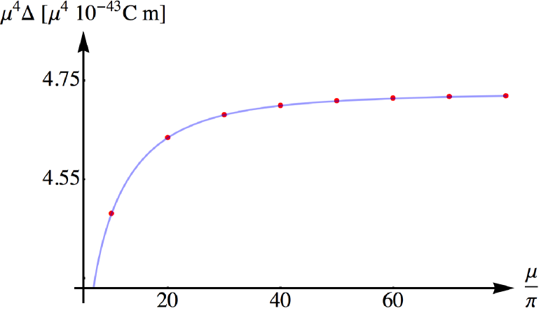
Figure 3: Plot as a function of $\mu$ of the scaled difference $\Delta=\mu^{4}(\mathcal{P}^{o}_{\Delta}-\mathcal{P}^{o}_{\Delta\,\mathrm{num}})$; here $\mathcal{P}^{o}_{\Delta}$ is defined by Eq. (127), and the difference is taken between the result from the asymptotic expansion based on Eq. (123) and the result from a numerical calculation $\mathcal{P}^{o}_{\Delta\,\mathrm{num}}$. The scaled difference approaches a constant as $\mu\to\infty$ and thus confirms the error estimate.

At this point we can go back to our full Hamiltonian including an EDM, which as we recall from Eq. (14) has the form

$$H(t)=\epsilon_{z}^{2}(t)\,F_{z}^{2}+\vec{\beta}(t)\cdot\vec{F}+\sigma_{F}\,\epsilon_{z}(t)\,F_{z}\,.$$ (118)

The electron EDM $d_{\textrm{e}}$ enters the dimensionless EDM coupling $\sigma_{F}=-d_{\textrm{e}}R/(F\,A_{\rm S}\,E_{S})$; it is assumed to be very small and we only need to include this effect in first order. We use a time-evolution operator for the EDM part of the Hamiltonian in Eq. (14),

$$\mathcal{W}=1-{\mathrm{i}}\int_{-\tau}^{\tau}\sigma_{F}\,\epsilon_{z}(t)\,F_{z}\,{\mathrm{d}}t\equiv 1+{\mathrm{i}}\,D\,F_{z}\,,$$ (119)

where we have defined

$$D=-\sigma_{F}\int_{-\tau}^{\tau}\epsilon_{z}(t)\,{\mathrm{d}}t\,,$$ (120)

where $\sigma_{F}$ has been defined in Eq. (15). The EDM term adds the $D$ term to our observable,

$${P(\theta)} /{4}=$$

$$D\!\biggl{[}\!\! \;\sum_{M=1,3}\!\!\!{p}_{M}\!\left<\Phi_{0}\right|\!F_{z}\!\left|\mathrm{Re}(R_{z})a_{M}\right>\!\!\langle\mathrm{Im}(R_{z})a_{M}|\Phi_{0}\rangle$$

$$-\!\!\!\!\! \sum_{M=0,2,4}\!\!\!\!\!{p}_{M}\!\left<\Phi_{0}\right|\!F_{z}\!\left|\mathrm{Im}(R_{z})a_{M}\right>\!\langle\mathrm{Re}(R_{z})a_{M}|\Phi_{0}\rangle\biggr{]}$$

$$-\frac{1}{\mu^{2}}\!\biggl{[}\! \,\,\sum_{M=1,3}\!\!\!{p}_{M}\!\left<\Phi_{0}\right|\!\sum_{j=1}^{3}\!\mathcal{M}_{2,2}^{(j)}(4)\,\mathcal{B}^{(j)}_{2,2}\!\left|\mathrm{Re}(R_{z})a_{M}\right>$$

$$\qquad\times\langle\mathrm{Im}(R_{z})a_{M}\left|1\right|\Phi_{0}\rangle$$ (121)

$$-\!\!\!\! \sum_{M=0,2,4}\!\!\!\!\!{p}_{M}\!\left<\Phi_{0}\right|\sum_{j=1}^{3}\mathcal{M}_{2,2}^{(j)}(4)\mathcal{B}^{(j)}_{2,2}\left|\mathrm{Im}(R_{z})a_{M}\right>$$

$$\qquad\times\langle\mathrm{Re}(R_{z})a_{M}\left|1\right|\Phi_{0}\rangle$$

$$+\!\!\!\! \;\sum_{M=1,3}\!\!\!{p}_{M}\!\left<\Phi_{0}\left|\mathcal{M}_{1,1}(4)\mathcal{B}_{1,1}\right|\mathrm{Re}(R_{z})s_{M}\right>$$

$$\qquad\times\left<\mathrm{Im}(R_{z})s_{M}\left|\mathcal{N}_{1,1}(4)\mathcal{G}_{1,1}\right|\Phi_{0}\right>$$

$$-\!\!\!\! \;\sum_{M=2,4}\!\!\!{p}_{M}\left<\Phi_{0}\left|\mathcal{M}_{1,1}(4)\mathcal{B}_{1,1}\right|\mathrm{Im}(R_{z})s_{M}\right>$$

$$\qquad\times\left<\mathrm{Re}(R_{z})s_{M}\left|\mathcal{N}_{1,1}(4)\mathcal{G}_{1,1}\right|\Phi_{0}\right>\biggr{]}\!+\!\mathcal{O}(\mu^{-4})\,.$$

In this expression, we now take a closer look at the terms and realize that the important difference between $\mathcal{B}_{2,2}^{(2)}$ and $\mathcal{B}_{2,2}^{(3)}$ is that $\mathcal{B}_{2,2}^{(2)}$ reverses sign when the direction of the externally applied electric field is reversed while $\mathcal{B}_{2,2}^{(3)}$ stays the same. The signal in which we are interested is $D$, which also changes sign when the electric field is reversed. So, if we measure $P(\theta)$ twice, once with the electric field along the $z$ direction, and again with the electric field in the $-z$ direction, and subtract the results, then all electric field even terms are canceled in $P(\theta)$. For the electric field odd part of $P(\theta)$, we find

$$\mathcal{P}^{o}(\theta)={} \frac{1}{2}\bigl{(}P(\theta)_{+E}-P(\theta)_{-E}\bigr{)}$$ (122)

$${}={} 4\!\!\!\sum_{M=1,3}\!\!\!{p}_{M}\left<\mathrm{Im}(R_{z})a_{M}|\Phi_{0}\right>\left<\Phi_{0}\right|DF_{z}$$

$$\!\!\!-\!{\mu^{-2}}\bigl{[}\mathcal{M}_{2,2}^{(1)}(4)\mathcal{B}^{(1,o)}_{2,2}\!+\!\mathcal{M}_{2,2}^{(2)}(4)\mathcal{B}^{(2)}_{2,2}\bigr{]}\left|\mathrm{Re}(R_{z})a_{M}\right>$$

$${}-{} 4\!\!\!\!\!\sum_{M=0,2,4}\!\!\!\!\!{p}_{M}\left<\mathrm{Re}(R_{z})a_{M}|\Phi_{0}\right>\left<\Phi_{0}\right|DF_{z}$$

$$\!\!\!-\!{\mu^{-2}}\bigl{[}\mathcal{M}_{2,2}^{(1)}(4)\mathcal{B}^{(1,o)}_{2,2}\!+\!\mathcal{M}_{2,2}^{(2)}(4)\mathcal{B}^{(2)}_{2,2}\bigr{]}\left|\mathrm{Im}(R_{z})a_{M}\right>$$

$$\quad+\mathcal{O}(\mu^{-4})\,.$$

For $F=4$, the observable $P(\theta)[\Phi_{0}]$ corresponding to two different initial states $\big{|}\Phi_{0}\big{>}$ evaluates to

$$\mathcal{P}^{o}(\theta)\left[\frac{1}{\sqrt{2}}(\left|4,4\right>+\left|4,-4\right>)\right]=$$ (123)

$$\sin(8\theta)\biggl{(}\!4D\!-\frac{2\mathcal{B}^{(1,o)}_{2,2}}{49\mu^{2}}\!\biggr{)}\!\frac{1}{32}\bigl{(}35{p}_{0}\!+28{p}_{2}\!+{p}_{4}\!-56{p}_{1}\!-8{p}_{3}\bigr{)}$$

$$\;+\frac{1}{15}\frac{\mathcal{B}^{(2)}_{2,2}}{\mu^{2}}\biggl{(}\sin(4\theta)\cos(2\theta)\left[{p}_{1}-{p}_{3}\right]$$

$$\qquad\quad\;\,-\frac{1}{4}\sin(2\theta)\cos(4\theta)\left[5{p}_{0}-4{p}_{2}-{p}_{4}\right]\biggr{)}+\mathcal{O}(\mu^{-4})\,,$$

$$\mathcal{P}^{o}(\theta)\left[\frac{1}{\sqrt{2}}(\left|4,2\right>+\left|4,-2\right>)\right]=$$ (124)

$$\sin(4\theta)\biggl{(}\!2D-\frac{9\mathcal{B}^{(1,o)}_{2,2}}{25\mu^{2}}\!\biggr{)}\frac{1}{8}\bigl{(}5{p}_{0}+4{p}_{2}+7{p}_{4}-2{p}_{1}-14{p}_{3}\bigr{)}$$

$$\;+\frac{1}{15}\frac{\mathcal{B}^{(2)}_{2,2}}{\mu^{2}}\biggl{(}\sin(2\theta)\cos(4\theta)\left[{p}_{1}-{p}_{3}\right]$$

$$\qquad\quad\;\,-\frac{1}{4}\sin(4\theta)\cos(2\theta)\left[5{p}_{0}-4{p}_{2}-{p}_{4}\right]\biggr{)}+\mathcal{O}(\mu^{-4})\,.$$

Here, the electric-field odd part $\mathcal{B}^{(1,o)}_{2,2}$ of $\mathcal{B}^{(1)}_{2,2}$ is

$$\mathcal{B}^{(1,o)}_{2,2}=\left\{\begin{array}[]{ll}-2\int_{-\tau}^{\tau}x_{o}^{\prime}(t)y_{e}(t)\,{\mathrm{d}}t&\textrm{for}\;k_{\epsilon}+k_{\beta}\;\textrm{even}\\[4.30554pt] +2\int_{-\tau}^{\tau}x_{o}(t)y_{e}^{\prime}(t)\,{\mathrm{d}}t&\textrm{for}\;k_{\epsilon}+k_{\beta}\;\textrm{odd}\,,\end{array}\right.$$ (125)

and $\mathcal{B}^{(2)}_{2,2}$ is given by

$$\mathcal{B}^{(2)}_{2,2}=x_{o}(-\tau)y_{e}(-\tau)\,.$$ (126)

The set of probabilities ${p}_{M}$ with $M=0$, $1$, $2$, $3$, and $4$ can be chosen from among the sets in Table 1 by choosing the frequency of the analysis laser. The angle $\theta$ can be varied continuously by changing the inclination of the axis of linear polarization of the analysis laser.

In the expressions above the angle $\theta$ is in the range $[0,\pi/2]$. The term in $\mathcal{B}_{2,2}^{(2)}$ is even in $\theta$ about the midpoint $\theta=\pi/4$, and the term in $\mathcal{B}^{(1,o)}_{2,2}$ and in the electron EDM contribution $D$ are both odd. The odd linear combination for data for different angles $\theta$,

$$\begin{split}\mathcal{P}^{o}_{\Delta}=\frac{1}{2}\biggl{\{}&\mathcal{P}^{o}\left(\frac{\pi}{16},\frac{1}{\sqrt{2}}\,(\left|4,4\right>+\left|4,-4\right>)\right)\\ {}-{}&\mathcal{P}^{o}\left(\frac{7\pi}{16},\frac{1}{\sqrt{2}}(\left|4,4\right>+\left|4,-4\right>)\right)\biggr{\}}\end{split}$$ (127)

both cancels any contribution from $\mathcal{B}_{2,2}^{(2)}$ and maximizes the sensitivity of what remains to $D$. The even linear combination isolates $\mathcal{B}_{2,2}^{(2)}$. Once isolated, $\mathcal{B}^{(1,o)}_{2,2}$ can be tuned to be of small magnitude because it depends on the vertical component of the static magnetic field at the entrance to the electric field plates, which can be tuned by varying a current in a nearby coil.

Once $\mathcal{B}_{2,2}^{(2)}$ has been tuned to be of small magnitude, canceled, or both, the remaining systematic $\mathcal{B}^{(1,o)}_{2,2}$ can be canceled by taking the right linear combination of data for different initial states, as shown by Eqs. (123) and (124). This systematic can also be isolated, and then tuned to be of small magnitude by varying the vertical component of the static magnetic field, in this case at a location away from the entrance to the electric field plates.

A big advantage of the proposed observable is that there are no EDM mimicking effects of order $1/\mu^{3}$, which had it been present would have been relevant on the proposed level of sensitivity. It is not yet necessary to cancel or control EDM-mimicking effects of order $1/\mu^{4}$, particularly since in practice, our experimental accuracy will be limited by other systematic effects such as magnetic Johnson noise, as for example discussed in Ref. Mu2005 .

IV EXPERIMENTAL REALIZATION

So far, we have considered a rather idealized model of an atomic fountain. In order to make sure that an actual experiment is not hindered by systematic effects arising from more realistic conditions, we now consider systematic effects outside the model.

The effect on $\mathcal{P}^{o}_{\Delta}$ of a linear vertical gradient in the component of the magnetic field in the $y$-direction is explored numerically in Fig. 4. Because of the parabolic rise and fall of the atoms while within the electric field, such a gradient results in the atomic rest frame as a $y$ component of the magnetic field that is of the form $\beta_{y}({\rm static})(a+bt^{2})$ for constants $a$ and $b$. In Fig. 4, we use atomic data for the atom ${}^{133}{\rm Cs}$ and find that $\mathcal{P}^{o}_{\Delta}$ depends linearly on both $a$ and $b$. The numerical calculation which produces Fig. 4 has also been verified against the analytic result found in Eq. (125) for the EDM-mimicking effect $\mathcal{B}_{2,2}^{(1,o)}$.

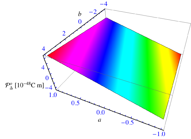
Figure 4: Plot of a numerical result for the signal function given in Eq. (127), denoted as $\mathcal{P}^{o}_{\Delta}$, for ¹³³Cs, depending on $a$ and $b$. The $a$ and $b$ parameters describe the magnetic field in the $y$ direction as $\beta_{y}(t)=\beta_{y}(\mathrm{static})\;(a+bt^{2})$.

A similar numerical analysis is shown in Fig. 5.of the dependence of $\mathcal{P}^{o}_{\Delta}$ on a deviation of $\delta k_{\epsilon}$ and $\delta k_{\beta}$ from their respective phase adjustment to integer multiples $k_{\epsilon}$ and $k_{\beta}$ of $\pi$. The results suggest that the deviations should not exceed $\sim 10^{-3}$ for the error in the signal to remain within the limits set forth by our target accuracy of $\sim 10^{-9}$.

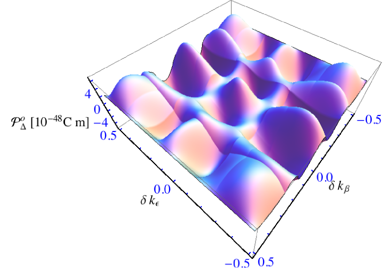
Figure 5: Plot of a numerical result for the signal of Eq. (127), $\mathcal{P}^{o}_{\Delta}$, for ¹³³Cs depending on the deviations $\delta k_{\epsilon}$ of $k_{\epsilon}$ and $\delta k_{\beta}$ of $k_{\beta}$ from the phase adjustment in Eqs. (29) and (30), respectively.

In a real as opposed to an ideal fountain, the common point of state preparation and analysis does not occur at the edge of a step-function rise of the electric field. In practice both will occur at a point where the electric field is essentially zero, well below the entrance to the electric field plates where over a transition region whose vertical extent is the order of the plate spacing the electric field ramps from zero to a constant value. Between the common point and the beginning of the transition region, the atoms will be in the presence of a stray magnetic field that will effect a small rotation of the atomic state. In the transition region the combination of a significant motional magnetic field and a stray magnetic field, acting while the tensor Stark splittings are still small, generates among other effects an additional rotation about the $z$ axis that can mimic the rotation effected by an electron EDM. All such effects influence the atom both on its way into the full electric field and on its way out.

The additional effects can be studied by defining time-evolution operators for each of these processes. For the transition region, we may expand the time-evolution operator in terms of the short (dimensionless) transition time $\aleph$, which is small against the overall time $T$ the atom spends in the fountain. The rotation that occurs (about some arbitrary axis) before the atom enters the transition region may be expanded in the small rotation angle $\delta$. We end up with three parameters $1/\mu$, $\aleph$, and $\delta$, which in the natural units of this work are all dimensionless, small, and in a practical apparatus roughly of the same order of magnitude, $\sim 1/\mu$. We can thus systematically model EDM-mimicking effects up to a desired order in the small parameters. Terms of third order are relevant on the proposed level of sensitivity. A detailed discussion of this expansion, which follows a formalism akin to the calculation of the time-evolution operators considered here, remains beyond the scope of the current paper. Technical details, which will be given elsewhere, reveal that the dominant terms in $\aleph$ and in $\delta$ do not mimic an EDM and can thus be discarded. The remaining effects can be satisfactorily described on the level of our proposed target accuracy.

One might also speculate about the effect of a departure of the atomic motion within the electric field from a straight line, as well as the effects of misalignments of the axes of propagation or of polarization of the laser used for state preparation and analysis. The first of these effects can be included within our approach by adding an electric-field odd but time-even motional magnetic field in the $y$ direction. We have carried out a calculation of this effect whose detailed discussion again is beyond the scope of the current paper. We find that only the field-dependent functions change but not the coefficient matrices. Our proposed cancellation mechanism is based solely on the coefficient matrices and so not affected by a change in the values of the field-dependent functions. Misalignments of the direction of propagation of a laser or of its axis of polarization can be modeled by representing the actual laser as being an ideal laser rotated by a small angle; this small angle can be treated as a small parameter that affects the time evolution of the atoms just as do $1/\mu$, $\aleph$, and $\delta$. We have not found any effects that could possibly represent insurmountable difficulties at the level of our proposed target accuracy; the design of the experimental apparatus is in progress.

V FRANCIUM AND CESIUM SYSTEMS

The availability of accelerator sources has made possible the use francium (half-life 3 minutes) instead of cesium in the atomic fountain. The main advantage of francium is that the enhancement factor $R$ is about $9$ times larger in francium than in cesium (see Table 3). Furthermore, certain francium isotopes, especially ²¹¹Fr, have a higher total angular momentum, namely $F=5$, which reduces the relative size of the EDM-mimicking effects. Moreover, the higher tensor polarizability also leads to $\mu$ being larger and thereby speeds the convergence of the formalism presented here.

Here, we present the results of our time-ordered calculation for $F=3$, which covers the case of ²²¹Fr, and for $F=5$, which covers ²¹¹Fr. Only the coefficient matrices $\mathcal{N}$ and $\mathcal{M}$ differ from those for $F=4$; the corresponding field-dependent functions $\mathcal{B}$ and $\mathcal{G}$ are identical. In the asymptotic expansion of the unitary transformation $U$ to order $1/\mu^{2}$, those matrices not given for general $F$ in Sec. II are gathered in the Appendices E, F, G, and H of Ref. WuMuJe2012app . Here, we only present the results for our proposed observable $\mathcal{P}^{o}(\theta)[\Phi_{0}]$ for four initial states $\big{|}\Phi_{0}\big{>}$ for the two isotopes; results for some other initial states are given in Appendix I of Ref. WuMuJe2012app .

$$\begin{split}\mathcal{P}^{o}&(\theta)\left[\frac{1}{\sqrt{2}}\,\big{(}\big{|}3,3\big{>}+\big{|}3,-3\big{>}\big{)}\right]=\sin(6\theta)\biggl{(}3D-\frac{3\mathcal{B}_{2,2}^{(1,o)}}{50\mu^{2}}\biggr{)}\frac{1}{8}\left(15{p}_{1}+{p}_{3}-10{p}_{0}-6{p}_{2}\right)\\ &\quad\qquad\qquad\qquad\qquad\quad\;\,+\frac{15}{16}\frac{\mathcal{B}_{2,2}^{(2)}}{\mu^{2}}\biggl{(}2\sin(3\theta)\cos(\theta)\,\left[{p}_{0}-{p}_{2}\right]+\sin(\theta)\cos(3\theta)\,\left[{p}_{3}-{p}_{1}\right]\biggr{)}+\mathcal{O}(\mu^{-4})\,,\end{split}$$ (128)

$$\begin{split}\mathcal{P}^{o}&(\theta)\left[\frac{1}{\sqrt{2}}\,\big{(}\big{|}5,5\big{>}+\big{|}5,-5\big{>}\big{)}\right]=\sin(10\theta)\biggl{(}5D-\frac{5\mathcal{B}_{2,2}^{(1,o)}}{162\mu^{2}}\biggr{)}\!\frac{1}{128}\left(210{p}_{1}\!+45{p}_{3}\!+{p}_{5}\!-126{p}_{0}\!-120{p}_{2}\!-10{p}_{4}\right)\\ &\quad\quad+\frac{5}{7}\frac{1}{512}\frac{\mathcal{B}_{2,2}^{(2)}}{\mu^{2}}\biggl{(}2\sin(5\theta)\cos(3\theta)\left[7{p}_{0}-4{p}_{2}-3{p}_{4}\right]+\sin(3\theta)\cos(5\theta)\left[13{p}_{3}+{p}_{5}-14{p}_{1}\right]\biggr{)}+\mathcal{O}(\mu^{-4})\,,\end{split}$$ (129)

$$\begin{split}\mathcal{P}^{o}(\theta)\left[\big{|}3,0\big{>}\right]&=\sin(2\theta)\frac{\mathcal{B}_{2,2}^{(2)}}{\mu^{2}}\frac{5}{4}\left({p}_{3}-{p}_{1}\right)+\mathcal{O}(\mu^{-4})\,,\end{split}$$ (130)

$$\begin{split}\mathcal{P}^{o}(\theta)\left[\big{|}5,0\big{>}\right]&=\sin(2\theta)\frac{\mathcal{B}_{2,2}^{(2)}}{\mu^{2}}\frac{35}{16}\left(3{p}_{5}-{p}_{3}-2{p}_{1}\right)+\mathcal{O}(\mu^{-4})\,,\end{split}$$ (131)

The variable $D$ has been defined in Eq. (120) and incorporates the effect of the EDM in view of its dependence on $\sigma_{F}$ defined in Eq. (15). Equations (128) and (129) show that when $F$ is odd, initial states consisting of superpositions of states with equal $|M|$ do not exhibit the symmetry in $\theta$ around $\pi/2$ that when $F$ is even could be used to cancel the systematic effect $\mathcal{B}_{2,2}^{(2)}$. Measurements on the states $\big{|}F,0\big{>}$ are shown by equations (130) and (131) to be sensitive only to only to $\mathcal{B}_{2,2}^{(2)}$, which can therefore be measured and tuned to be small by changing the vertical component of the static magnetic field at the entrance to the electric field plates. Any residual effect can be separated from the values of $D$ and of the other systematic $\mathcal{B}_{2,2}^{(1,o)}$ either by combining data for different angles $\theta$, or by altering the laser frequency and combining data for different sets of values ${p}_{M}$. The sets accessible for $F=3$ and for $F=5$ may be found in Appendix B of Ref. WuMuJe2012app .

VI CONCLUSIONS

We set up the formalism for the theoretical description of the quantum dynamics of an alkali atom within an atomic fountain designed for an EDM experiment. The low velocity of the atoms inside a fountain reduces the motional magnetic field, which arises as the Lorentz transformation of the applied electric field, by a factor of $100$ compared to experiments on thermal atomic beams. In an atomic fountain the quantization axis is defined by the direction of the externally applied strong electric field, and is not defined by a magnetic field; we are therefore free to greatly reduce all magnetic fields and their attendant systematic errors by use of extensive magnetic shielding and nulling coils. Compared to many previous experiments these two features suppress effects that mimic the presence of an EDM, because such effects scale linearly with both the motional magnetic field and any stray field. We describe a theoretical calculation that identifies the remaining EDM-mimicking effects and devise schemes to eliminate them.

A crucial part of our formalism is writing the time evolution operator from time-ordered perturbation theory in terms of an analytic expansion in the inverse number of electric-field induced Rabi oscillations within the hyperfine manifold. When the magnetic fields in the $x$ and $y$ directions are zero, the time-evolution operator for a single hyperfine manifold is a diagonal matrix of phases $V$, which reduces to a simple rotation of the atomic system provided the cumulative electric and magnetic field phases of Eq. (29) and Eq. (30) are tuned to integer multiples of $\pi$.

The perturbing effects of stray magnetic fields in the $x$ and $y$ directions as well as the motional magnetic field in the $x$ direction, still without an EDM term, can be treated when the electric field is constant by expanding the correction term $W(t)$ in the formula for the time-evolution operator $U(t)=V(t)\,W(t)$ in an asymptotic expansion in inverse powers of $\mu=\epsilon_{z}^{2}$, where $\mu/(2\pi)$ describes the number of Rabi oscillations in the hyperfine manifold induced in the absence of perturbing fields. Under typical experimental conditions a value of $\mu$ on the order of one hundred can be obtained and so expansion is therefore rapidly converging. The expansion of $W$ to order $1/\mu^{2}$ requires consideration of terms of fourth order of perturbation theory; we present the expansion in terms of constant matrices multiplied by analytic functions of the stray and motional magnetic fields.

We then define an observable $P(\theta)$, which is a function of the angle of inclination of the linear polarization of the laser used to analyze the final state of the atom. This observable is sensitive to a rotation of the initial state about the electric field axis, as would be induced by the presence of an electron EDM. A transformation of the final state into pieces symmetric and antisymmetric with respect to two transformations $B$ and $S$ defined in Eqs. (47) and (48) proves that many contributions cancel. Critically it is proven that in the asymptotic expansion of $P$ only even powers of $1/\mu$ appear, so knowledge of the time development operator out to order $1/\mu^{2}$ suffices to compute $P$ with error $1/\mu^{4}$, not $1/\mu^{3}$.

After taking the difference for opposite signs of the electric field, besides the effect of an electron EDM only two systematic errors survive, which can both be isolated and canceled by combining data for polarization angles, laser frequencies, and initial states; moreover both systematic errors once measured can be tuned to be of small magnitude by imposing additional small magnetic fields. The systematics start intrinsically smaller than in previous experiments because of the smaller velocity of atoms in an atomic fountain, which reduces the magnitude of the motional magnetic field, and because in an atomic fountain with a large electric field a magnetic field is not required to define a quantization axis, so stray components of the magnetic field can be suppressed to the limit provided by the surrounding magnetic shielding.

The proposed apparatus is expected to detect an EDM on a level of $2\times 10^{-50}\,{\rm C\,m}$, or better. The limit is due to higher-order effects and due magnetic Johnson noise Mu2005 from the materials used in the apparatus.

References

- (1) E. M. Purcell and N. F. Ramsey, On the Possibility of Electric Dipole Moments for Elementary Particles and Nuclei, Phys. Rev. 78, 807 (1950).
- (2) L. D. Landau, Conservation Laws in Weak Interactions, JETP 5, 336 (1957), [Zh. Éksp. Teor. Fiz. 32, 405 (1957)].
- (3) G. Lüders and B. Zumino, Connection between Spin and Statistics, Phys. Rev. 110, 1450 (1958).
- (4) A. D. Sakharov, CP violation and baryonic asymmetry of the Universe, JETP Lett. 5, 24 (1967), [Pis’ma v ZhETF 5, 32 (1967)].
- (5) A. D. Sakharov, Violation of CP invariance, C asymmetry, and baryon asymmetry of the universe, Sov. Phys. Usp. 34, 392 (1991), [Usp. Fiz. Nauk 161, 61 (1991)].
- (6) M. Berkooz, Y. Nir, and T. Volansky, Baryogenesis from the Kobayashi-Maskawa Phase, Phys. Rev. Lett. 93, 051301 (2004).
- (7) N. Dombey and A. D. Kennedy, A calculation of the electron anapole moment, Phys. Lett. B 91, 428 (1980).
- (8) M. Pospelov and A. Ritz, Electric dipole moments as probes of new physics, Ann. Phys. (N.Y.) 318, 119 (2005).
- (9) L. Wolfenstein, T. Trippe, and C.-J. Lin, Tests of Conservation Laws, in Review of Particle Physics, K. Nakamura et al. [Particle Data Group], J. Phys. G 37, 075021 (2010).
- (10) R. N. Mohapatra, S. Antusch, K. S. Babu, G. Barenboim, M.-C. Chen, A. de Gouvêa, P. de Holanda, B. Dutta, Y. Grossman, A. Joshipura, B. Kayser, J. Kersten, Y. Y. Keum, S. F. King, P. Langacker, M. Lindner, W. Loinaz, I. Masina, I. Mocioiu, S. Mohanty, H. Murayama, S. Pascoli, S. T. Petcov, A. Pilaftsis, P. Ramond, M. Ratz, W. Rodejohann, R. Shrock, T. Takeuchi, T. Underwood, , and L. Wolfenstein, Theory of neutrinos: a white paper, Rep. Prog. Phys. 70, 1757 (2007).
- (11) M. Pospelov, A. Ritz, and Y. Santoso, Flavor- and CP-Violating Physics from New Supersymmetric Thresholds, Phys. Rev. Lett. 96, 091801 (2006).
- (12) R. Mahbubani and L. Senatore, Minimal model for dark matter and unification, Phys. Rev. D 73, 043510 (2006).
- (13) L. Senatore, Hierarchy from baryogenesis, Phys. Rev. D 73, 043513 (2006).
- (14) J. Hudson, D. Kara, I. Smallman, B. Sauer, M. Tarbutt, and E. Hinds, Improved measurement of the shape of the electron, Nature (London) 473, 493 (2011).
- (15) B. C. Regan, E. D. Commins, C. J. Schmidt, and D. DeMille, New Limit on the Electron Electric Dipole Moment, Phys. Rev. Lett. 88, 071805 (2002).
- (16) W. Fischler, S. Paban, and S. Thomas, Bounds on microscopic physics from P and T violation in atoms and molecules, Phys. Lett. B 289, 373 (1992).
- (17) S. Abel, S. Khalil, and O. Lebedev, EDM constraints in supersymmetric theories, Nucl. Phys. B 606, 151 (2001).
- (18) S. Khalil, CP Violation in Supersymmetric Theories, Int. J. Mod. Phys. A 18, 1697 (2003).
- (19) K. A. Olive, M. Pospelov, A. Ritz, and Y. Santoso, CP–odd phase correlations and electric dipole moments, Phys. Rev. D 72, 075001 (2005).
- (20) W. Bernreuther and M. Suzuki, The electric dipole moment of the electron, Rev. Mod. Phys. 63, 313 (1991), [Erratum Rev. Mod. Phys. 64 633(E) (1992)].
- (21) S. M. Barr, A Review of CP Violation in Atoms, Int. J. Mod. Phys. A 8, 209 (1993).
- (22) Y. Li, S. Profumo, and M. Ramsey-Musolf, A Comprehensive Analysis of Electric Dipole Moment Constraints on CP-violating Phases in the MSSM, J. High Energy Phys. 1008, 062 (2010).
- (23) N. Arkani-Hamed, S. Dimopoulos, G. Giudice, and A. Romanino, A comprehensive analysis of electric dipole moment constraints on CP-violating phases in the MSSM, Nucl. Phys. B 709, 3 (2005).
- (24) D. Chang, W.-F. Chang, and W.-Y. Keung, Electric dipole moment in the split supersymmetry models, Phys. Rev. D 71, 076006 (2005).
- (25) G. Giudice and A. Romanino, Electric dipole moments in split supersymmetry, Phys. Lett. B 634, 307 (2006).
- (26) H. E. Haber, Supersymmetry, Part 1 (Theory), revised October 2009, in Review of Particle Physics, C. Amsler et al., Phys. Lett. B 667, 1 (2008), available at the URL http://pdg.lbl.gov/2009/reviews/rpp2009-rev-susy-1-theory.pdf.
- (27) B. J. Wundt, C. T. Munger, and U. D. Jentschura, Quantum dynamics in atomic-fountain experiments for measuring the electric dipole moment of the electron with improved sensitivity: Supplemental Material, Supplement to Phys. Rev. X 2, 041009 (2012). The appendices contain a discussion of the expected signal in the experiment and varius matrices and subexpressions for higher-order terms in the expansion of the time-evolution operator . See http://link.aps.org/supplemental/10.1103/PhysRevX.2.041009
- (28) K. Nakamura et al. [Particle Data Group], Review of Particle Physics, J. Phys. G 37, 075021 (2010).
- (29) P. G. H. Sandars, Enhancement factor for the electric dipole moment of the valence electron in an alkali atom, Plenum 22, 290 (1966).
- (30) W. R. Johnson, D. S. Guo, M. Idrees, and J. Sapirstein, Weak-interaction effects in heavy atomic systems. II, Phys. Rev. A 34, 1043 (1986).
- (31) A. Shukla, B. P. Das, and J. Andriessen, Relativistic many-body calculation of the electric dipole moment of atomic rubidium due to parity and time-reversal violation, Phys. Rev. A 50, 1155 (1994).
- (32) H. S. Nataraj, B. K. Sahoo, B. P. Das, and D. Mukherjee, Intrinsic Electric Dipole Moments of Paramagnetic Atoms: Rubidium and Cesium, Phys. Rev. Lett. 101, 033002 (2008).
- (33) W. R. Johnson, D. S. Guo, M. Idrees, and J. Sapirstein, Weak-interaction effects in heavy atomic systems, Phys. Rev. A 32, 2093 (1985).
- (34) A.-M. Mårtensson-Pendrill and P. Öster, Calculations of atomic electric dipole moments, Phys. Scr. 36, 444 (1987).
- (35) A. C. Hartley, E. Lindroth, and A.-M. Mårtensson-Pendrill, arity non-conservation and electric dipole moments in caesium and thallium, J. Phys. B 23, 3417 (1990).
- (36) V. A. Dzuba and V. V. Flambaum, Calculation of the (T,P)-odd electric dipole moment of thallium and cesium, Phys. Rev. A 80, 062509 (2009).
- (37) T. M. R. Byrnes, V. A. Dzuba, V. V. Flambaum, and D. W. Murray, Enhancement factor for the electron electric dipole moment in francium and gold atoms, Phys. Rev. A 59, 3082 (1999).
- (38) D. Mukherjee, B. K. Sahoo, H. S. Nataraj, and B. P. Das, Relativistic Coupled Cluster (RCC) Computation of the Electric Dipole Moment Enhancement Factor of Francium Due to the Violation of Time Reversal Symmetry, J. Phys. Chem. A 113, 12549 (2009).
- (39) V. A. Dzuba, V. V. Flambaum, K. Beloy, and A. Derevianko, Hyperfine-mediated static polarizabilities of monovalent atoms and ions, Phys. Rev. A 82, 062513 (2010).
- (40) P. G. H. Sandars, Differential polarizability in the ground state of the hydrogen atom, Proc. Phys. Soc. 92, 857 (1967).
- (41) J. Kalnins, G. Lambertson, and H. Gould, Improved alternating gradient transport and focusing of neutral molecules, Rev. Sci. Instr. 73, 2557 (2002).
- (42) J. G. Kalnins, J. M. Amini, and H. Gould, Focusing a fountain of neutral cesium atoms with an electrostatic lens triplet, Phys. Rev. A 72, 043406 (2005).
- (43) J. G. Kalnins, Electrostatic end-field defocusing of neutral atoms and its compensation, Phys. Rev. ST Accel. Beams 14, 104201 (2011).
- (44) P. Fuentealba and O. Reyes, Polarizabilities and hyperpolarizabilities of the alkali metal atoms, J. Phys. B 26, 2245 (1993).
- (45) J. M. Amini, C. T. Munger, and H. Gould, Electron electric-dipole-moment experiment using electric-field quantized slow cesium atoms, Phys. Rev. A 75, 063416 (2007).
- (46) J. M. Amini, Electron Electric Dipole Moment Experiment using a Cold Cesium Fountain, doctoral thesis, University of California at Berkeley, 2006. See http://labs.adsabs.harvard.edu/ui/abs/2006PhDT……..91A.
- (47) C. M. Bender and S. A. Orszag, Advanced Mathematical Methods for Scientists and Engineers (McGraw-Hill, New York, NY, 1978).
- (48) The yields of available isotopes at the CERN ISOLDE experiment can be queried at the URL https://oraweb.cern.ch/pls/isolde/query_tgt. The element francium () is of particular interest for the current study.
- (49) The yields of available isotopes at the TRIUMF ISAC facility can be queried at the URL http://www.triumf.info/facility/research_fac/yield.php Francium () is of interest for the current study.
- (50) The TRIUMF ISAC Beam Development Plan (Status as of May 29, 2012), is available at the URL http://www.triumf.ca/sites/default/files/BeamDevelopmentPlan-2012-05-29.pdf.
- (51) J. Nolen, Project X Collaboration Meeting, Lawrence Berkeley National Laboratory, April 10–12, 2012; see the URL https://indico.fnal.gov/conferenceTimeTable.py?confId=5300#all.detailed.
- (52) S. Aubin, E. Gomez, L. A. Orozco, and G. D. Sprouse, High efficiency magneto-optical trap for unstable isotopes, Rev. Sci. Instr. 74, 4332 (2003).
- (53) D. Melconian, M. Trinczek, A. Gorelov, W. P. Alford, J. A. Behr, J. M. D’Auria, M. Dombsky, U. Giesen, K. P. Jackson, T. B. Swanson, and W. Wong, Release of from catcher foils, Nucl. Instrum. Methods A 538, 93 (2005).
- (54) C. T. Munger, Magnetic Johnson noise constraints on electron electric dipole moment experiments, Phys. Rev. A 72, 012506 (2005).