Multi-wavelength study of triggered star formation around mid-infrared bubble N14

Abstract

We present multi-wavelength analysis around mid-infrared (MIR) bubble N14 to probe the signature of triggered star formation as well as the formation of new massive star(s) and/or cluster(s) on the borders of the bubble by the expansion of the H ii region. Spitzer-IRAC ratio maps reveal that the bubble is traced by the polycyclic aromatic hydrocarbon (PAH) emission following an almost circular morphology except in the south-west direction towards the low molecular density environment. The observational signatures of the collected molecular and cold dust material have been found around the bubble. We have detected 418 young stellar objects (YSOs) in the selected region around the bubble N14. Interestingly, the detected YSO clusters are associated with the collected molecular and cold dust material on the borders of the bubble. One of the clusters is found with deeply embedded intermediate mass and massive Class I YSOs associated with one of the dense dust clumps in the east of the bubble N14. We do not find a good agreement between the dynamical age of the H ii region and the fragmentation time of the accumulated molecular materials to explain possible “collect-and-collapse” process around the bubble N14. Therefore, we suggest the possibility of triggered star formation by compression of the pre-existing dense clumps by the shock wave and/or small scale Jeans gravitational instabilities in the collected materials. We have also investigated 5 young massive embedded protostars (8 to 10 M_⊙) and 15 intermediate mass (3 to 7 M_⊙) Class I YSOs which are associated with the dust and molecular fragmented clumps at the borders of the bubble. We conclude that the expansion of the H ii region is also leading to the formation of these intermediate and massive Class I YSOs around the bubble N14.

1 Introduction

Massive stars (M $>$ 8 M_⊙) have the ability to interact with the surrounding cloud with their energetic wind, UV ionizing radiation and an expanding H ii region (Zinnecker & Yorke, 2007). In recent years, MIR shells or bubbles around the expanding H ii regions are recognised as the sites to observationally investigate the conditions of sequential/triggered star formation (Elmegreen & Lada, 1977; Elmegreen, 2010, and references therein) and the formation of new massive star(s) and/or cluster(s) as well. Two mechanisms have been proposed to explain the observed star formation due to influence of massive star(s): “collect and collapse” (Elmegreen & Lada, 1977; Whitworth et al., 1994) and radiation-driven implosion (RDI; Bertoldi, 1989; Lefloch & Lazareff, 1994). In the “collect and collapse” scenario, the H ii region expands and accumulates molecular material between the ionization and the shock fronts. With time the collected material becomes unstable and fragments into several clumps and lead to the formation of new generation of stars, as an effect of the shocks. In the RDI model, the expanding H ii region supply enough external pressure to initiate collapse of a pre-existing dense clump in the molecular material.

In this work, we present a multi-wavelength study of a MIR bubble N14 associated with IRAS 18134-1652, from the catalog of Churchwell et al. (2006, 2007) around the Galactic H ii region G014.0-00.1. The bubble N14 is situated at a near distance of 3.5 kpc (Beaumont & Williams, 2010) and is associated with the water maser near ($\sim$ 33 arcsec) to the IRAS position (Codella et al., 1994). Lockman (1989) reported the velocity of ionized gas (v_LSR) to be about 36 km s^-1 near to the IRAS position, using a hydrogen recombination line study. Beaumont & Williams (2010) and Deharveng et al. (2010) studied several MIR bubbles including the N14 using James Clerk Maxwell Telescope (JCMT) ¹²CO(J=3-2) line and APEX Telescope Large Area Survey of the Galactic plane at 870 $\mu$m (ATLASGAL) 870 $\mu$m continuum observations, respectively. Beaumont & Williams (2010) also reported 20 cm Multi-Array Galactic Plane Imaging Survey (MAGPIS) radio continuum data around the N14. Beaumont & Williams (2010) estimated molecular gas velocity to be about 40.3 km s^-1 associated with the bubble N14 with velocity dispersion of 2.8 km s^-1. They also listed about six O9.5 stars to produce observed MAGPIS 20 cm integrated flux ($\sim$ 2.41 Jy) for the H ii region associated with the bubble N14. Deharveng et al. (2010) found three dense clumps around the bubble N14 and stated that the bubble is broken in the direction of the low density region.

Previous studies on this region therefore clearly reveal the presence of molecular, cold dust as well as ionized emissions in the bubble. In this paper, we present multi-wavelength observations to study the interaction of H ii region with the surrounding interstellar medium (ISM). Our study will allow us to investigate the star formation especially the identification of embedded populations and also explore whether there is any evidence to form stars by the triggering effect of the H ii region around the bubble N14.

In Section 2, we introduce the archival data and data reduction procedures used for the present study. In Section 3, we examine the structure of the MIR bubble N14 in different wavelengths and the interaction of massive stars with its environment using various Spitzer MIR ratio maps. In this section, we also describe the selection of young population, their distribution around the bubble, identification of ionizing candidates and discuss the triggered star formation scenario on the borders of the bubble. In Section 4, we summarize our conclusions.

2 Available data and data reduction

Archival deep near-infrared (NIR) HK_s images and a catalog around the bubble N14 were obtained from the UKIDSS 6^th archival data release (UKIDSSDR6plus) of the Galactic Plane Survey (GPS) (Lawrence et al., 2007). It is to be noted that there is no GPS J band observation available for the bubble N14. UKIDSS observations were made using the UKIRT Wide Field Camera (WFCAM; Casali et al., 2007) and fluxes were calibrated using Two Micron All Sky Survey (2MASS; Skrutskie et al., 2006). The details of basic data reduction and calibration procedures are described in Dye et al. (2006) and Hodgkin et al. (2009), respectively. Magnitudes of bright stars (H $\leqslant$ 11.5 mag and K_s $\leqslant$ 10.5 mag) were obtained from the 2MASS, due to saturation of UKIDSS bright sources. Only those sources are selected for the study which have photometric magnitude error of 0.1 and less in each band to ensure good photometric quality.
We obtained narrow-band molecular hydrogen (H₂; 2.12 $\mu$m; 1 - 0 S(1)) imaging data from UWISH2 survey (Froebrich et al., 2011). We followed a procedure similar to that described by Varricatt (2011) to obtain the final continuum-subtracted H₂ image using GPS K_s image.
The Spitzer Space Telescope Infrared Array Camera (IRAC (Ch1 (3.6 $\mu$m), Ch2 (4.5 $\mu$m), Ch3 (5.8 $\mu$m) and Ch4 (8.0 $\mu$m); Fazio et al., 2004) and Multiband Imaging Photometer (MIPS (24 $\mu$m); Rieke et al., 2004) archival images were obtained around the N14 region from the “Galactic Legacy Infrared Mid-Plane Survey Extraordinaire” (GLIMPSE; Benjamin et al., 2003; Churchwell et al., 2009) and “A 24 and 70 Micron Survey of the Inner Galactic Disk with MIPS” (MIPSGAL; Carey et al., 2005) surveys. MIPSGAL 24 $\mu$m image is saturated close to the IRAS position inside the bubble N14. We used GLIMPSE-I Spring ’07 highly reliable Point-Source Catalog and also performed aperture photometry on all the GLIMPSE images (plate scale of 0.6 arcsec/pixel) using a 2.4 arcsec aperture and a sky annulus from 2.4 to 7.3 arcsec using IRAF for those sources detected in images but the photometric magnitudes are not available in the GLIMPSE-I catalog. The IRAC/GLIMPSE photometry is calibrated using zero magnitudes including aperture corrections, 18.5931 (Ch1), 18.0895 (Ch2), 17.4899 (Ch3) and 16.6997 (Ch4), obtained from IRAC Instrument Handbook (Version 1.0, February 2010).
We obtained 20 cm radio continuum map (resolution $\sim$ 6 arcsec) from Very Large Array MAGPIS survey (Helfand et al., 2006) to trace the ionized region around the N14. The molecular ¹²CO(J=3-2) (rest frequency 345.7959899 GHz) spectral line public processed archival data was also utilized in the present work. The CO observations (project id: M10BD02) were taken on 22 August 2010 at the 15 m JCMT using the HARP array. Archival BOLOCAM 1.1 mm (Aguirre et al., 2011) image (with effective FWHM Gaussian beam size of $\sim$ 33 arcsec) was also used in the present work.

3 Results and Discussion

3.1 Multi-wavelength view of the bubble N14

Figure 1 shows the selected region ($\sim$ 12 $\times$ 8.6 arcmin²) around the bubble N14, made of the 3-color composite image using GLIMPSE (8.0 $\mu$m (red) & 4.5 $\mu$m (green)) and UKIDSS K_s (blue). The 8 $\mu$m band contains the two strongest PAH features at 7.7 $\mu$m and 8.6 $\mu$m, which are excited in the photodissociation region (or photon-dominated region, or PDR). The PDRs are the interface between neutral & molecular hydrogen and traced by PAH emissions. PAH emission is also known to be the tracer of ionization fronts. The positions of IRAS 18134-1652 (+) and water maser ($\times$) (Codella et al., 1994) are marked in the figure. Figure 1 displays an almost circular morphology of the MIR bubble N14 prominently around the IRAS 18134-1652. These bubble structures are not seen in any of the UKIDSS NIR images, but prominently visible in all GLIMPSE images. JCMT molecular gas (JCMT CO 3-2) emission contours are also overlaid on the Fig. 1 with 20, 40, 60, 80 and 95 % of the peak value i.e. 60.43 K km s^-1. The peak positions of the three detected 870 $\mu$m dense clumps (Deharveng et al., 2010) are also marked by a big star symbol in the figure. Figure 2 shows a color composite image made using MIPSGAL 24 $\mu$m (red), GLIMPSE 8 $\mu$m (green), and 3.6 $\mu$m (blue) images, overlaid by BOLOCAM 1.1 mm emission by solid yellow contours. MIPS 24 $\mu$m image is saturated near to the IRAS position, but a few point sources are also seen around the bubble. MAGPIS 20 cm radio continuum emission is also overlaid in Figure 2 by black contours. The cold dust emission at 1.1 mm is very dense and prominent at the borders of the bubble. It is clearly seen that the peaks of 870 $\mu$m, 1.1 mm dust emission and CO molecular gas emissions are spatially coincident along the borders of the bubble (see Figs. 1 & 2). The 24 $\mu$m and 20 cm images trace the warm dust and ionized gas in the region, respectively. It is obvious from Figure 2 that the PDR region (traced by 8 $\mu$m) encloses 24 $\mu$m dust and 20 cm ionized emissions inside the bubble and indicates the presence of dust and gas in and around the H ii region (see e. g. Watson et al., 2008, for N10, N21, and N49 bubbles).

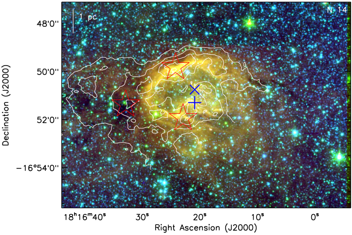
Figure 1: Three color composite image (size $\sim$ 12 $\times$ 8.6 arcmin²; central coordinates: $\alpha_{2000}$ = 18^h 16^m 18^s.9, $\delta_{2000}$ = -16^° 51^′ 25^″.2) of the selected region around the bubble N14, using Spitzer-GLIMPSE images at 8.0 $\mu$m (red), 4.5 $\mu$m (green) and UKIDSS K_s (blue) in log scale. Archival JCMT molecular ¹²CO (3-2) gas emission contours are also overlaid on the image with 20, 40, 60, 80 and 95 % of the peak value i.e. 60.43 K km s^-1. The positions of the three 870 $\mu$m dust clumps from Deharveng et al. (2010) are marked by big red star symbols in the image. The scale bar on the top left shows a size of 1 pc at the distance of 3.5 kpc. The positions of IRAS 18134-1652 (+) and water maser ($\times$) are marked in the figure.

Figure 2: 20 cm contours in black color around the bubble N14 obtained from the MAGPIS survey, overlaid on a color composite image made using the 24 $\mu$m (red), 8 $\mu$m (green), and 3.6 $\mu$m (blue) images. The 20 cm contour levels are 40, 55, 70, 85 and 95 % of the peak value i.e. 0.0115 Jy/ beam. BOLOCAM 1.1 mm emission is also shown by solid yellow contours with 20, 30, 40, 55, 70, 85 and 95 % of the peak value i.e. 1.07 Jy/ beam. The peak positions of BOLOCAM 1.1 mm clumps are shown by triangle symbols obtained from the Bolocam Galactic Plane Survey (BGPS) catalog. The other marked symbols are similar to those shown in Fig. 1 (see text for more details). MIPS 24 $\mu$m image is saturated near the IRAS position.

3.2 PAH emission and the Collected material

In recent years, Spitzer-IRAC bands and ratio maps are utilized to study the interaction of massive stars with its immediate environment (Povich et al, 2007). The IRAC bands contain a number of prominent atomic and molecular lines/features such as H₂ lines in all channels (see Table 1 from Smith & Rosen, 2005), Br$\alpha$ 4.05 $\mu$m (Ch2), Fe ii 5.34 $\mu$m (Ch3), Ar ii 6.99 $\mu$m and Ar iii 8.99 $\mu$m (Ch4) (see Reach et al., 2006). We know that the Spitzer-IRAC bands, Ch1, Ch3 and Ch4, contain the PAH features at 3.3, 6.2, 7.7 and 8.6 $\mu$m, whereas Ch2 (4.5 $\mu$m) does not include any PAH features. Therefore, IRAC ratio (Ch4/Ch2, Ch3/Ch2 and Ch1/Ch2) maps are being used to trace out the PAH features in massive star forming (MSF) regions (e.g. Povich et al, 2007; Watson et al., 2008; Kumar & Anandarao, 2010; Dewangan et al., 2012) due to UV radiation from massive star(s). In order to make the ratio maps, we generate residual frames for each band removing point sources by choosing an extended aperture (12.2 arcsec) and a larger sky annulus (14.6 - 24.4 arcsec; Reach et al., 2005) in IRAF/DAOPHOT software (Stetson, 1987). These residual frames are then subjected to median filtering with a width of 4 pixels and smoothing by 9 $\times$ 9 pixels using the boxcar algorithm. Figures 3a and 3b represent the IRAC ratio maps, Ch3/Ch2 and Ch4/Ch2 around the bubble N14, respectively. The ratio contours are also overlaid on the maps for better clarity and insight (see Fig. 3). Both the ratio maps clearly trace the prominent PAH emissions and subsequently the extent of PDRs in the region. IRAC ratio maps reveal that the bubble is traced by the PAH emission following an almost circular morphology except in south-west direction towards the low molecular density environment, which was also reported by Deharveng et al. (2010).
The emission contours of dust (ATLASGAL 870 $\mu$m and BOLOCAM 1.1 mm) and molecular gas (JCMT CO 3-2) exhibit the evidence of collected material along the bubble (see Figs. 1, 2 and 3). Deharveng et al. (2010) tabulated the positions of three 870 $\mu$m dust condensations with their respective molecular velocity using the NH₃(1,1) inversion line between 39 to 41.5 km s^-1. These values are also consistent with Beaumont & Williams (2010), who also reported velocity for the bubble N14 ($\sim$ 40.3 km s^-1). These velocity ranges of molecular gas are also compatible with the ionized gas velocity ($\sim$ 36 km s^-1) obtained by the hydrogen recombination line study around the H ii region (Lockman, 1989), which confirms the physical association of the molecular material and the H ii region. It is also to be noted that the peaks of cold dust and molecular gas emission at different locations possibly indicate the fragmentation of collected materials into different individual clumps around the bubble. The evidence of collected material along the bubble is further confirmed by the detection of the H₂ emission (see Figure 4). Figure 4 represents the continuum-subtracted H₂ image at 2.12 $\mu$m and reveals that the H₂ emission surrounds the H ii region along the bubble, forming a PDR region, which may be collected due to the shock. In brief, the PAH emission, cold dust emission, molecular CO gas and shocked H₂ emissions are coincident along the bubble.

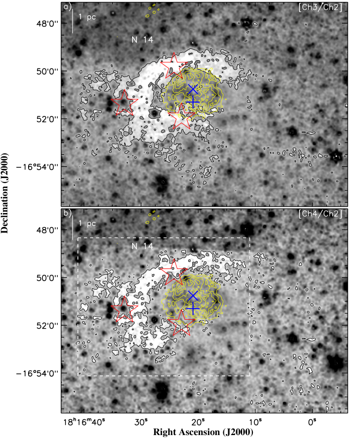
Figure 3: a) GLIMPSE Ch3/Ch2 ratio map of the region around N14 (similar area as shown in Fig. 1). The ratio Ch3/Ch2 value is found to be “7–8” and “8.5–10” in the bubble interior and for the brightest part of the PDR respectively. The Ch3/Ch2 ratio contours are also overlaid on the image with a level of 8.3, a representative value between “7–8.5”. b) The Ch4/Ch2 ratio map of the region is shown here. The ratio Ch4/Ch2 value for the brightest part of the PDR and the interior is “30–34” and “23–25” respectively. The Ch4/Ch2 ratio contours are also overlaid on the image with a level of 27.8, a representative value between “25–30”. The white dashed box is shown as a zoomed-in view in Fig. 4. MAGPIS 20 cm radio contours in yellow color are also overlaid in both the figures. The marked symbols and levels of radio contours on the figure are similar to those shown in Fig. 1.

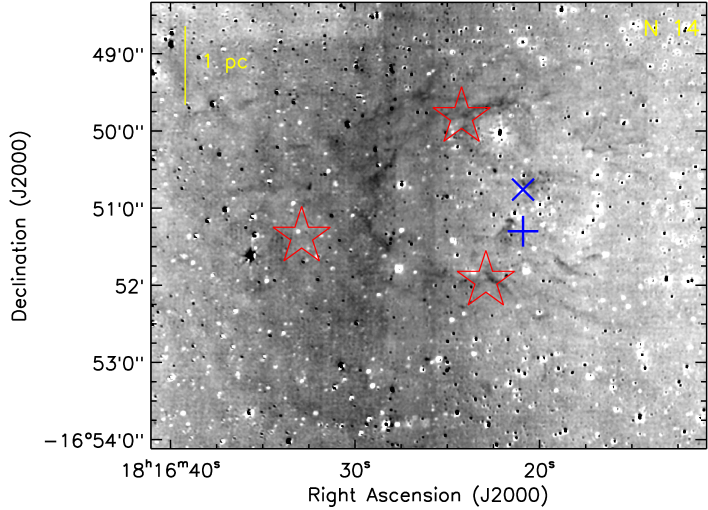
Figure 4: Zoomed-in inverted gray-scale continuum-subtracted H₂ image at 2.12 $\mu$m around N14 (size $\sim$ 7.2 $\times$ 5.7 arcmin²; as shown by a dashed box in Fig. 3b). The H₂ image clearly indicates the detected H₂ emission (dark features as seen in GLIMPSE images) in the selected region around N14. The marked symbols are similar to those shown in Fig. 1. The continuum-subtracted H₂ image is processed through median filtering with a width of 4 pixels and smoothened by 4 $\times$ 4 pixels using boxcar algorithm to trace the faint features in the image.

3.3 Photometric analysis of point-like sources towards N14

In order to trace ongoing star formation activity around the bubble N14, we have identified YSOs using NIR and GLIMPSE data.

3.3.1 Selection of YSOs

We have used Gutermuth et al. (2009) criteria based on four IRAC bands to identify YSOs and various possible contaminants (e.g. broad-line AGNs, PAH-emitting galaxies, shocked emission blobs/knots and PAH-emission-contaminated apertures). These YSOs are further classified into different evolutionary stages (i.e. Class I, Class II, Class III and photospheres) using slopes of the IRAC spectral energy distribution (SED). Fig. 5a shows the IRAC color-color ([3.6]-[4.5] vs [5.8]-[8.0]) diagram for all the identified sources. We find 33 YSOs (15 Class 0/I; 18 Class II), 621 photospheres and 78 contaminants in the selected region around the bubble N14. The details of YSO classifications can be found in Dewangan & Anandarao (2011). We have also applied criteria ([3.6]-[4.5] = 0.7 and [4.5]-[5.8] = 0.7; Hartmann et al. (2005); Getman et al. (2007)) to identify protostars (Class I) among the sources, which are detected in three IRAC/GLIMPSE bands, but not in the 8.0 $\mu$m band and rest of the remaining sources are subjected to SED criteria (see Dewangan & Anandarao, 2011) to select the Class II and Class III sources. We identify 186 additional YSOs (10 Class 0/I; 176 Class II) through color-color diagram using three GLIMPSE bands in the region (see Fig. 5b).
GLIMPSE 3.6 and 4.5 $\mu$m bands are more sensitive for point sources than GLIMPSE 5.8 and 8.0 $\mu$m images. Therefore, a larger number of YSOs can be identified using a combination of UKIDSS NIR HK_s photometry with GLIMPSE 3.6 and 4.5 $\mu$m (i.e. NIR-IRAC) photometry, where sources are not detected in IRAC 5.8 and/or 8.0 $\mu$m band (Gutermuth et al., 2009). We followed the criteria given by Gutermuth et al. (2009) to identify YSOs using H, K_s, 3.6 and 4.5 $\mu$m data. We have found 199 additional YSOs (185 Class II and 14 Class I) using NIR-IRAC data (see Fig. 5c).
Finally, we have obtained a total of 418 YSOs (379 Class II and 39 Class I) using NIR and GLIMPSE data in the region.

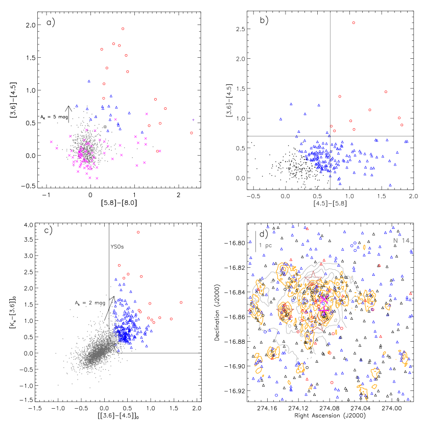
Figure 5: a) Color-color diagram (CC-D) using Spitzer-IRAC four bands for all the sources identified within the region shown in Fig. 1. The extinction vector for A_K = 5 mag is shown by an arrow, using average extinction law from Flaherty et al. (2007). The dots in gray color around the centre (0,0) locate the stars with only photospheric emissions. The open squares (black), open triangles (blue) and open circles (red) represent Class III, Class II and Class 0/I sources respectively, classified using the $\alpha_{IRAC}$ criteria. The “$\times$” symbols in magenta color show the identified PAH-emission-contaminated apertures in the region. The PAH galaxy contamination source is also marked by a violet cross (+) symbol in the diagram (see the text). b) CC-D of the sources detected in three IRAC/GLIMPSE bands, except 8.0 $\mu$m. The small filled cirlces (black), open triangles (blue) and open circles (red) represent Class III, Class II and Class 0/I sources respectively (see the text for YSOs selection critria). c) Figure shows the de-reddened [K_s - [3.6]]₀ $vs$ [[3.6] - [4.5]]₀ CC-D using NIR and GLIMPSE data. The selected region shown by the solid lines represents the location of YSOs. The extinction vector for A_K = 2 mag is shown by an arrow, calculated using the average extinction law from Flaherty et al. (2007). Open red circles and open blue triangles represent Class I and Class II sources respectively. d) Plot represents the spatial distribution of all identified YSOs in the selected region around N14. The YSO surface density contours are plotted for 6, 9, 14, 20 and 26 YSOs/pc², from outer to inner side (see text for details). The open circles and open triangles show the Class I and Class II sources respectively. The YSOs identified using four IRAC, three IRAC and NIR-IRAC data are shown by red, black and blue colors respectively. The JCMT ¹²CO (3-2) contours in gray color and marked symbols are similar to those shown in Fig. 1.

3.3.2 Spatial distribution of YSOs

To study the spatial distribution of YSOs, we generated the surface density map of all YSOs using a 5 arcsec grid size, following the same procedure as given in Gutermuth et al. (2009). The surface density map of YSOs is constructed using 6 nearest-neighbor (NN) YSOs for each grid point. Fig. 5d shows the spatial distribution of all identified YSOs (Class I and Class II) in the region. The contours of YSO surface density are also overlaid on the map. The levels of YSO surface density contours are 6 (2.1$\sigma$), 9 (3.2$\sigma$), 14 (4.9$\sigma$), 20 (7.0$\sigma$) and 26 (9.1$\sigma$) YSOs/pc², increasing from the outer to the inner region. We have also calculated the empirical cumulative distribution (ECD) as a function of NN distance to identify the clustered YSOs in the region. Using the ECD, we estimate the distance of inflection $d_{c}$ = 0.54 pc (0.0088 degrees at 3.5 kpc) for the region for a surface density of 6 YSOs/pc² (see Dewangan & Anandarao, 2011, for details of $d_{c}$ and ECD). We find that about 23% (98 out of 418) YSOs are present in clusters. Figure 5d reveals that the distribution of YSOs is mostly concentrated in and around the bubble, having peak density of about 20 YSOs/pc² (see also Figure 6), while YSO density of about 8 YSOs/pc² (2.8$\sigma$) is also seen around the east and west regions close to the low density molecular gas and dust emission (see Figure 6). It is also to be noted that the YSOs clustering is seen along the PDR region, on the borders of the bubble. The correlation of cold dust, molecular gas, ionized gas and YSO surface density is shown in Figure 6. The association of YSOs with the collected materials around the region further reveals the ongoing star formation on the borders of the bubble.

In addition, we have checked the possibility of intrinsically “red sources” contamination, such as asymptotic giant branch (AGB) stars in our YSO sample. Recently, Robitaille et al. (2008) prepared an extensive catalog of such red sources based on the Spitzer GLIMPSE and MIPSGAL surveys. They showed that two classes of sources are well separated in the [8.0 - 24.0] color space such that YSOs are redder than AGB stars in this space (see also Whitney et al., 2008). Firstly, we applied red source criteria for all our selected YSOs having 4.5 $\mu$m and 8.0 $\mu$m detections. We find 19 out of 33 YSOs ($\sim$ 57%) as possible intrinsically “red sources” and then further utilized [8.0 - 24.0] color space to identify the AGB contaminations from selected “red sources”. We have taken MIPS 24 $\mu$m magnitude for our selected sources from Robitaille et al. (2008), wherever it is available and also extracted a few more sources from archival MIPSGAL 24 $\mu$m image. We performed aperture photometry on MIPSGAL 24 $\mu$m image using IRAF with a 7 arcsec aperture & a sky annulus from 7 to 13 arcsec. Zero points and aperture corrections were adopted from MIPS Instrument Handbook Version 3, March 2011, for selected aperture. MIPS 24 $\mu$m image is saturated close to the IRAS position, however, a few point sources are seen around the bubble. Therefore, we obtained MIPS 24 $\mu$m magnitudes for only 9 YSOs (7 Class I and 2 Class II) identified as red sources. Finally, we identified two likely AGB contaminations out of 9 red sources, following the criteria suggested by Robitaille et al. (2008), which are located away from the identified YSO clusters (see Figure 6). We have not considered these likely AGB contaminations for further analysis.

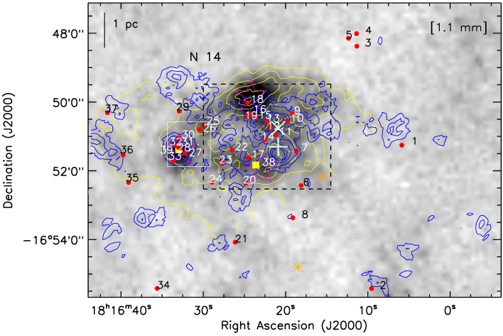
Figure 6: The spatial distribution of YSOs, dust emission and molecular gas in the selected region around N14. BOLOCAM 1.1 mm image is overlaid with contours of YSO surface density (blue; similar levels as presented in Fig. 5d) and JCMT CO 3-2 (yellow; similar levels as shown in Fig. 1) data. All Class I YSOs (see subsection 3.3.3) are also marked (red circles) and labeled as 1,….,37 on the image (see Table 1). Two selected sources (s38 and s39) are shown by filled yellow squares and labeled, which are associated with the peaks of molecular gas and dust emission around the bubble. The position of two likely AGB contaminations is also marked by orange asterisks on the image. Two boxes are shown as a zoomed-in view in Fig. 7.

3.3.3 SED modeling of Class I YSOs

In this subsection, we present SED modeling of all 37 identified Class I YSOs (designated as s1,…..,s37) as well as two selected YSOs (s38 and s39) associated with the peak of molecular gas and dust clumps around the bubble, in our selected region around N14, to derive their various physical parameters using an on-line SED modeling tool (Robitaille et al., 2006, 2007). It is interesting to note that “s39” is a deeply embedded source (prominently seen in 24 $\mu$m image), detected only in 5.8 $\mu$m and longer wavelength bands. NIR and Spitzer IRAC/GLIMPSE photometric magnitudes for these selected YSOs are listed in Table 1 along with IRAC spectral indices ($\alpha_{IRAC}$) and are also labeled in Fig. 6. Spitzer 24 $\mu$m magnitudes are also listed for selected YSOs, wherever it is available. Figs. 7a and  7b show the zoomed-in 3 color composite image using GLIMPSE (5.8 $\mu$m (red) & 4.5 $\mu$m (green)) and UKIDSS K_s (blue) around the east of the bubble close to the peak of a dense clump and around the bubble, respectively. Fig. 7a clearly exhibits the location of a deeply embedded source “s39” along with other identified Class I sources close to the peak of a cold dust emission.

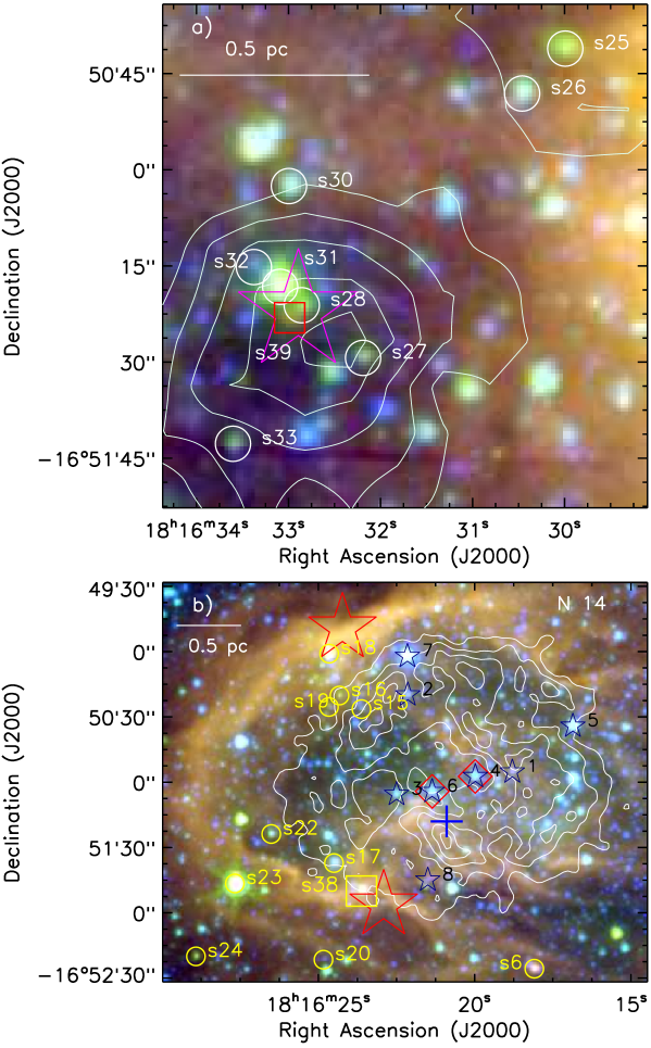
Figure 7: Three color composite image (UKIRT K_s (blue) and GLIMPSE 4.5 $\mu$m (green), 5.8 $\mu$m (red)) of the two zoomed-in regions around the bubble N14. a) Figure clearly exhibits the location of a deeply embedded source “s39” along with other identified Class I sources close to the peak of cold dust emission (see white solid box in Fig. 6). b) The MAGPIS 20 cm contours are overlaid on the zoomed-in region (dashed box in Fig. 6) with similar levels as shown in Fig. 2 close to the bubble N14 (size $\sim$ 3.7 $\times$ 3.1 arcmin²). The 8 selected main sequence stars as probable ionizing candidates (see subsection 3.3.4) are also marked (black star symbols) and labeled as 1,….,8 on the image (see Table 2). The diamonds in red color are identified as the O-type ionizing stars (#4 and #6) inside the bubble. Some of Class I YSOs in yellow color are also marked and labeled on the figure.

Fig. 7b presents the zoomed-in view around the bubble with the positions of a few identified YSOs (such as s17, s18 and s38, along with other identified Class I YSOs).
IRAC spectral indices were calculated using a least squares fit to the IRAC flux points in a log($\lambda$) versus log($\lambda$F_λ) diagram for those sources that are detected in atleast 3 IRAC bands (see Dewangan & Anandarao, 2011, for details). The SED model tool requires a minimum of three data points with good quality as well as the distance to the source and visual extinction value. These models assume an accretion scenario with a central source associated with rotationally flattened infalling envelope, bipolar cavities, and a flared accretion disk, all under radiative equilibrium. The model grid consists of 20,000 models of two-dimensional Monte Carlo simulations of radiation transfer with 10 inclination angles, resulting in a total of 200,000 SED models. The grid of SED models covers the mass range from 0.1 to 50 M_⊙. Only those models are selected that satisfy the criterion $\chi^{2}$ - $\chi^{2}_{best}$ $<$ 3, where $\chi^{2}$ is taken per data point. The plots of SED fitted models are shown in Fig. 8 for 9 out of 39 selected YSOs associated with the molecular and dust clumps. The weighted mean values of the physical parameters (mass and luminosity) along with the standard deviations derived from the SED modeling for all the selected sources are given in Table 1. The SED results clearly show that the YSOs having higher luminosity represent more massive candidates. The table also contains the number of models that satisfy the $\chi^{2}$ criterion as mentioned above. The derived SED model parameters show that the average values of mass and luminosity of the 39 selected sources are about 4.8 M_⊙ and 1817.1 L_⊙, respectively. Our SED result shows that the source “s4” is the most luminous and massive YSO ($\sim$ 20.5 M_⊙) among all selected YSOs away from the bubble and is saturated in the GLIMPSE 8 $\mu$m image. It is however tabulated as an OH selected AGB/post-AGB candidate by Sevenster (2002) using 1612 MHz masing OH line profile. The YSO surface density contours clearly trace a clustering of Class I YSOs (s27-28, s30-33 and s39) with $\sim$ 20 YSOs/pc² associated with the dense dust clump at the eastern border of the bubble N14 along with other peaks of YSO surface density (see Figs 6, 7a and Table 1). It is found that about 5 young massive embedded YSOs (s6, s18, s23, s28 and s31) with a mass range of 8 to 10 M_⊙ and about 15 intermediate mass YSOs (s7, s9-10, s12, s14, s16-17, s19, s22, s25-26, s30, s33, s38-39) with mass range of 3 to 7 M_⊙ are associated with the molecular and dust fragmented clumps at the borders of the bubble (see Figs. 6, 7 and Table 1). It is interesting to note that the sources s18, s28, s31, s38 and s39 are associated with the peak of dust clumps at the border of the bubble and three of them (s18, s28 and s31) are possibly young massive protostars. Finally, the SED modeling results favor ongoing star formation around the region with detection of YSOs as well as some massive protostars in their early phase of formation.

Recently, Kryukova et al. (2012) studied a relationship between bolometric luminosity and MIR luminosity (integrated from 1.25 $\mu$m to 24 $\mu$m) of Spitzer identified protostars in nine nearby molecular clouds, independent of SED modeling. We have also computed the MIR luminosity (L_MIR) of our selected sources from integrating the SED using their available photometric infrared data (see Table 1 for L_MIR). However, the estimated MIR luminosity of our selected sources is underestimated because of the lack of 24 $\mu$m and longer wavelength data for most of the sources. Therefore, we prefer to use model derived SED physical parameters (like mass and luminosity) over luminosity derived independently of SED modeling for our selected sources. It is known that the physical parameters obtained from SED modeling are not unique but indicative. We therefore used only mass of selected sources for their relative comparison in terms of mass.

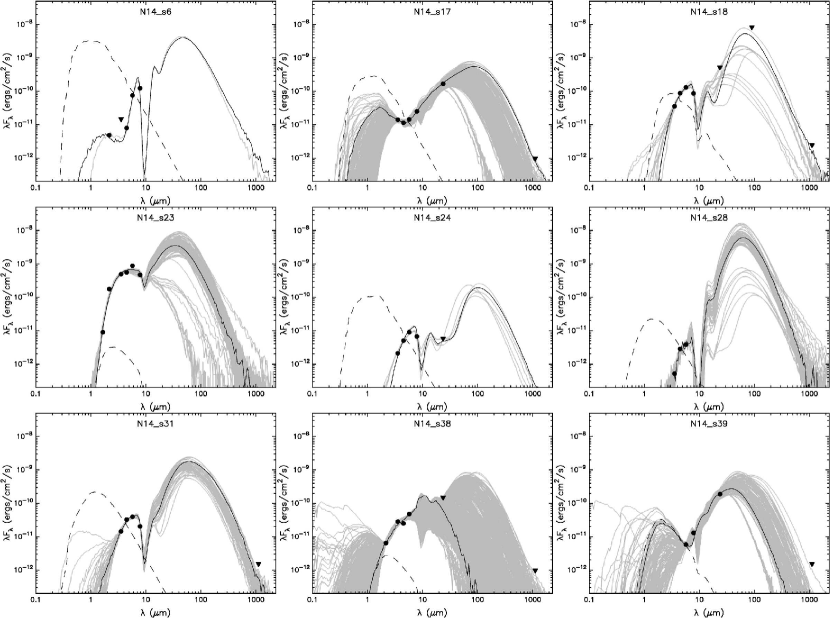
Figure 8: The SED plots of 9 out of 39 selected YSOs associated with the molecular and dust clumps are shown here. Filled circles are observed fluxes of good quality (with filled triangles as upper limits) taken from the archives or published literature (see text for more details) and the curves show the fitted model with criteria $\chi^{2}$ - $\chi^{2}_{best}$ $<$ 3. The thin black curve corresponds to the best fitting model. The dashed curves represent photospheric contributions.

3.3.4 Ionizing Candidates

The presence of both PAH emission around the bubble and radio emission inside the bubble clearly suggest the presence of the ionizing source(s) with UV radiation close to the centre of the bubble. One can find more details regarding identification of ionizing candidate(s) inside the bubble in Pomarés et al. (2009) and Ji et al. (2012). It is to be noted that no ionizing stars are reported for this bubble. Beaumont & Williams (2010) listed about six O9.5 stars to produce observed 20 cm integrated flux ($\sim$ 2.41 Jy) for the H ii region associated with the bubble N14. Therefore, we followed suggestions of Pomarés et al. (2009) and Ji et al. (2012) to trace the ionizing candidate(s) inside the bubble N14 using 2MASS and GLIMPSE photometric magnitudes. We selected 8 candidates (designated as #1,…..,#8) to search for O-type star(s) inside the bubble based on their detections in J band to 5.8 $\mu$m or longer wavelength bands (see Fig. 7b and Table 2). All selected candidates are marked and labeled in Fig. 7b. We calculated the absolute JHK_s magnitude for each candidate using their 2MASS apparent J, H, and K_s magnitudes. 2MASS photometry is used here due to non availability of GPS J band photometry. We used a distance of 3.5 kpc and estimated the extinction for each source from the NIR color color diagram (CC-D). We followed the extinction law given by Indebetouw et al. (2005) (A_J/A_V = 0.284, A_H/A_V = 0.176 and A_K/A_V = 0.114) and used the intrinsic colors (J - H)₀ (= -0.11) and (H - K)₀ (= -0.10) obtained from Martins & Plez (2006). We compared the derived absolute JHK_s magnitudes with those listed by Martins & Plez (2006) for our selected candidates, and found two O-type candidates (#4 and #6) inside the bubble. We also checked their evolutionary stages using CC-D (see subsection 3.3.1) and found that all the sources are main sequence stars except source #3, which is identified as a Class I YSO and designated as s14 in Table 1. The positions of the 8 selected candidates are tabulated in Table 2 with their 2MASS NIR & GLIMPSE apparent magnitudes, calculated visual extinction, estimated absolute JHK_s magnitudes and the possible spectral class obtained from the comparison of absolute magnitude of each candidate with the listed values of Martins & Plez (2006).

3.4 Star formation scenario

We have found evidence of collected material along the bubble and also ongoing formation of YSOs on the borders of the bubble. The YSO clusters and embedded YSOs discovered are associated with the peak of molecular and cold dust material collected on the borders of the bubble. The morphology and distribution of YSOs suggest that the bubble N14 is a site of star formation possibly triggered by the expansion of the H ii region. In recent years, the triggered star formation process, especially “collect and collapse” mechanism has been studied extensively on the borders of many H ii regions such as Sh 2-104, RCW 79, Sh 2-212, RCW 120, Sh 2-217, G8.14+0.23 (Deharveng et al., 2003, 2008, 2009; Zavagno et al., 2006, 2010; Brand et al., 2011; Dewangan et al., 2012). In order to check the “collect and collapse” process as the triggering mechanism around N14, we have calculated the dynamical age (t_dyn) of the H ii region and compared it with an analytical model by Whitworth et al. (1994). We have estimated the age of the H ii region at a given radius R, using the following equation (Dyson & Williams, 1980):

$$t_{dyn}=\left(\frac{4\,R_{s}}{7\,c_{s}}\right)\,\left[\left(\frac{R}{R_{s}}\right)^{7/4}-1\right]$$ (1)

where c_s is the isothermal sound velocity in the ionized gas (c_s = 10 km s^-1) and R_s is the radius of the Strömgren sphere, given by R_s = (3 N_uv/4$\pi n^{2}_{\rm{0}}\alpha_{B}$)^1/3, where the radiative recombination coefficient $\alpha_{B}$ = 2.6 $\times$ 10^-13 (10⁴ K/T)^0.7 cm³ s^-1 (Kwan, 1997). In this calculation, we have used $\alpha_{B}$ = 2.6 $\times$ 10^-13 cm³ s^-1 for the temperature of 10⁴ K. N_uv is the total number of ionizing photons per unit time emitted by ionizing stars and “n₀” is the initial particle number density of the ambient neutral gas. We have adopted the Lyman continuum photon flux value (N_uv =) of 2.34 $\times$ 10⁴⁸ ph s^-1 (logN_uv = 48.36) from Beaumont & Williams (2010) for an electron temperature, distance and integrated 20 cm (1.499 GHz) flux density of 10⁴ K, 3.5 kpc, and 2.41 Jy respectively. We calculated the mean H₂ number density near the H ii region using archival ¹²CO zeroth moment map or column density map. In general, the zeroth moment map (in unit of K km s^-1) is created by integrating the brightness temperature over some velocity range. We derived the column density using the formula $N_{\rm H_{2}}$ (cm^-2) = $X$ $\times$ $W_{\rm CO}$, assuming the molecular clumps/cores are approximately spherical in shape. We used the CO–H₂ conversion factor (also called $X$ factor) for dense gas as 6 $\times$ 10²⁰ cm^-2 K^-1 km^-1 s from Shetty et al. (2011). We find almost a closed circular structure of integrated CO line emission ($W_{\rm CO}$) (typical value of $\sim$ 23.43 K km s^-1) using archival column density map, which traces well the bubble around the H ii region. The mean H₂ number density is obtained to be 2071.5 cm^-3 using the relation $N_{\rm H_{2}}$ (cm^-2)/$L$ (cm), where $L$ is the molecular core size of about 6.79 $\times$ 10¹⁸ cm ($\sim$ 2.2 pc) near the H ii region. The estimated mean H₂ number density could be under-estimated because of not considering the fact that the ¹²CO (3–2) transition can be (partly) optical thick in nature and also assuming a spherical structure in the calculation. Using N_uv, a radius of the H ii region (R =) 2.48 pc, and n₀ = 2071.5 cm^-3, we have obtained t_dyn $\sim$ 0.74 Myr using Equation 1. The timescale of H ii region expansion is actually not an easy issue. There is the long-standing problem of the lifetime of Galactic ultra-compact (UC) H ii regions. Wood & Churchwell (1989) observationally reported that the typical lifetime of UC H ii regions is about 10⁵ years, but the lifetime of an expanding UC H ii region (i.e. the timescale to reach pressure equilibrium with the surrounding environment) is estimated to be about 10⁴ years, for 10 km s^-1 expansion velocity of ionized gas, with a typical radius of $\sim$ 0.1 pc. So, the difference between these timescales is known as the lifetime problem of UC H ii regions. This lifetime problem might have implications in the present case even if it is only the UC H ii region which is living too long. Therefore, our estimated timescale should be considered with a caution. Following, the Whitworth et al. (1994) analytical model for the “collect and collapse” process, we have estimated a fragmentation time scale (t_frag) of 1.27 - 2.56 Myr for a turbulent velocity (a_s) of 0.2 - 0.6 km s^-1 in the collected layer. We find that the dynamical age is smaller than the fragmentation time scale for n₀ = 2071.5 cm^-3. We have checked the variation of t_frag and t_dyn with initial density (n₀) of the ambient neutral medium and found that if t_dyn is larger than t_frag, then ambient density (n₀) should be larger than 3610, 5710, 6700 and 7700 cm^-3 for different turbulent velocity (a_s) values of 0.2, 0.4, 0.5 and 0.6 km s^-1 respectively. We have also estimated the kinematical time scale of the molecular bubble of about 1.57 Myr ($\sim$ 4.5 pc/ 2.8 km s^-1), assuming bubble size of about 4.5 pc and velocity dispersion $\sim$ 2.8 km s^-1 from ¹²CO(J=3-2) map (see Beaumont & Williams, 2010). The comparison of the dynamical age of the H ii region with the kinematical time scale of expanding bubble and the fragmentation time scale, does not support the fragmentation of the molecular materials into clumps due to “collect and collapse” process around the bubble. Also, the average age of Class 0/I sources is reported to be about 0.10–0.44 Myr (see Evans et al., 2009), which is less than the fragmentation time scale of the molecular materials into clumps. Therefore, we suggest the possibility of triggered star formation by compression of the pre-existing dense clumps by the shock wave and/or small scale Jeans gravitational instabilities in the collected materials. The YSO surface density contours clearly trace a clustering of Class I YSOs (s27-28, s30-33 and s39), with three intermediate mass (s30, s33 and s39) and two massive embedded sources (s28 and s31) associated with the dense dust clump at the eastern border of the bubble N14 (see Fig. 7a and Table 1). We have also found that the s18 & s38 sources are also associated with the peak of different dust clumps around the bubble and the source “s18” is identified as a new young massive protostar.

4 Conclusions

We have explored the triggered star formation scenario around the bubble N14 and its associated H ii region using multi-wavelength observations. We find that there is a clear evidence of collected material (molecular and cold dust) along the bubble around the N14 region. The surface density of YSOs reveals ongoing star formation and clustering of YSOs associated with the borders of the bubble. We conclude that the YSOs are being formed on the border of the bubble possibly by the expansion of the H ii region. We further investigated the “collect-and-collapse” process for triggered star formation around N14 using the analytical model of Whitworth et al. (1994). We have found that the dynamical age ($\sim$ 0.74 Myr) of the H ii region is smaller, and the kinematical time scale of the bubble ($\sim$ 1.57 Myr) is comparable to the fragmentation time scale ($\sim$ 1.27 - 2.56 Myr) of accumulated gas layers in the region for 2071.5 cm^-3 ambient density. The comparison of the dynamical age with the kinematical time scale of expanding bubble and the fragmentation time scale does not support the fragmentation of the molecular materials into clumps due to the “collect and collapse” process around N14, but suggests the possibility of triggered star formation by compression of the pre-existing dense clumps by the shock wave and/or small scale Jeans gravitational instabilities in the collected materials. The YSO surface density contours clearly trace a clustering of Class I YSOs ($\sim$ 7 Class I sources with $\sim$ 20 YSOs/pc²) associated with the dense dust clump at the eastern border of the bubble N14. Also 5 young massive embedded protostars (about 8 to 10 M_⊙) and 15 intermediate mass (about 3 to 7 M_⊙) Class I YSOs are associated with the dust and molecular fragmented clumps at the borders of the bubble. It seems that the expansion of the H ii region is also leading to the formation of these intermediate and massive Class I YSOs around the bubble N14.

References

- Aguirre et al. (2011) Aguirre J. E., Ginsburg A. G., Dunham M. K., et al., 2011, ApJS, 192, 4
- Beaumont & Williams (2010) Beaumont C. N., Williams J. P., 2010, ApJ, 709, 791
- Bertoldi (1989) Bertoldi F., 1989, ApJ, 346, 735
- Benjamin et al. (2003) Benjamin R. A.,Churchwell E., Babler B. L., et al., 2003, PASP, 115, 953
- Brand et al. (2011) Brand J., Massi F., Zavagno A., Deharveng L., Lefloch B., 2011, A&A, 527, 62
- Carey et al. (2005) Carey S. J., et al., 2005, BAAS, 37, 1252
- Casali et al. (2007) Casali M., Adamson A., Alves de Oliveira C., Almaini O., Burch K., Chuter T., Elliot J., et al., 2007, A&A, 467, 777
- Churchwell et al. (2006) Churchwell E., Povich M. S., Allen D., et al., 2006, ApJ, 649, 759
- Churchwell et al. (2007) Churchwell E., Watson D. F., Povich M. S., et al., 2007, ApJ, 670, 428
- Churchwell et al. (2009) Churchwell E.,Babler B. L., Meade M. R., et al., 2009, PASP, 121, 213
- Codella et al. (1994) Codella C., Felli M., Natale V., Palagi F., Palla F., 1994, A&A, 291, 261
- Deharveng et al. (2003) Deharveng L., Lefloch B., Zavagno A., et al., 2003, A&A, 408, L25
- Deharveng et al. (2008) Deharveng L., Lefloch B., Kurtz S., et al., 2008, A&A, 482, 585
- Deharveng et al. (2009) Deharveng L., Zavagno A., Schuller F., et al., 2009, A&A, 496, 177
- Deharveng et al. (2010) Deharveng L., Schuller F., Anderson L. D. et al., 2010, A&A, 523, 6
- Dewangan & Anandarao (2011) Dewangan L. K., Anandarao B. G, 2011, MNRAS, 414, 1526
- Dewangan et al. (2012) Dewangan L. K., Ojha D. K., Anandarao B. G., Ghosh S. K., Chakraborti S., 2012, accepted in ApJ, arXiv:1207.6842
- Dye et al. (2006) Dye S., Warren S. J., Hambly N. C., Cross N. J. G., Hodgkin S. T., Irwin M. J., Lawrence A., et al., 2006, MNRAS, 372, 1227
- Dyson & Williams (1980) Dyson J. E., Williams D. A., 1980, Physics of the interstellar medium (New York, Halsted Press, p. 204)
- Fazio et al. (2004) Fazio G. G. et al., 2004, ApJS, 154, 10
- Elmegreen (2010) Elmegreen B. G., 2010, Ecole Evry Schatzman (EAS) Publications Series, 51, 45
- Elmegreen & Lada (1977) Elmegreen, B. G., Lada, C. J., 1977, ApJ, 214, 725
- Evans et al. (2009) Evans, N. J., II, Dunham, M. M., Jrgensen, J. K., et al., 2009, ApJS, 181, 321
- Flaherty et al. (2007) Flaherty K. M., Pipher J. L., Megeath S. T., Winston E. M., Gutermuth R. A., Muzerolle J., Allen L. E., Fazio, G. G., 2007, ApJ, 663, 1069
- Froebrich et al. (2011) Froebrich D., Davis C. J., Ioannidis G., et al., 2011, MNRAS, 413, 480
- Hartmann et al. (2005) Hartmann L., Megeath S. T., Allen L., et al., 2005, ApJ, 629, 881
- Helfand et al. (2006) Helfand D. J., Becker R. H., White R. L., Fallon A., Tuttle S., 2006, AJ, 131, 2525
- Hodgkin et al. (2009) Hodgkin S. T., Irwin M. J., Hewett P. C., Warren S. J., 2009, MNRAS, 394, 675
- Getman et al. (2007) Getman K. V., Feigelson E. D., Garmire G., Broos P., Wang J., 2007, ApJ, 654, 316
- Gutermuth et al. (2009) Gutermuth R. A., Megeath S. T., Myers P. C., Allen L. E., Pipher J. L., Fazio G. G., 2009, ApJS, 184, 18
- Indebetouw et al. (2005) Indebetouw R., Mathis J. S., Babler B. L., et al., 2005, ApJ, 619, 931
- Ji et al. (2012) Ji W.-G., Zhou J.-J, Esimbek J., et al., 2012, arXiv:1206.2762v1
- Kumar & Anandarao (2010) Kumar Dewangan Lokesh, Anandarao B. G., 2010, MNRAS, 407, 1170
- Kryukova et al. (2012) Kryukova, E.,Megeath, S. T., Gutermuth, R. A, et al., 2012, ApJ, 144, 31
- Kwan (1997) Kwan J., 1997, ApJ, 489, 284
- Lawrence et al. (2007) Lawrence A., Warren S. J., Almaini O., et al. 2007, MNRAS, 379, 1599
- Lefloch & Lazareff (1994) Lefloch, B., Lazareff, B. 1994, A&A, 289, 559
- Lockman (1989) Lockman F. J., 1989, ApJS, 71, 469
- Martins & Plez (2006) Martins F., Plez B., 2006, A&A, 457, 637
- Pomarés et al. (2009) Pomarés M., Zavagno A., Deharveng L., et al., 2009, A&A, 494, 987
- Povich et al (2007) Povich M. S., Stone J. M., Churchwell E., et al., 2007, ApJ, 660, 346
- Reach et al. (2005) Reach W. T., Megeath S. T., Cohen M., et al. 2005, PASP, 117, 978
- Reach et al. (2006) Reach W. T., Rho J., Tappe A., et al., 2006, AJ, 131, 1479
- Rieke et al. (2004) Rieke G. H. et al., 2004, ApJS, 154, 25
- Robitaille et al. (2006) Robitaille T. P., Whitney B. A., Indebetouw R., Wood K., Denzmore P., 2006, ApJS, 167, 256
- Robitaille et al. (2007) Robitaille T. P., Whitney B. A., Indebetouw R., Wood K., 2007, ApJS, 169, 328
- Robitaille et al. (2008) Robitaille T. P., Meade M. R., Babler B. L., et al., 2008, AJ, 136, 2413
- Sevenster (2002) Sevenster M. N., 2002, ApJ, 123, 2772
- Shetty et al. (2011) Shetty, R., Glover, S. C., Dullemond, C. P., Klessen, R. S., 2011, MNRAS, 412, 1686
- Skrutskie et al. (2006) Skrutskie M. F., Cutri R. M., Stiening R., Weinberg M. D., Schneider S., Carpenter J. M., Beichman C., et al., 2006, AJ, 131, 1163
- Smith & Rosen (2005) Smith M. D., Rosen A., 2005, MNRAS, 357, 1370
- Stetson (1987) Stetson P. B., 1987, PASP, 99, 191
- Varricatt (2011) Varricatt W. P., 2011, A&A, 527, 97
- Watson et al. (2008) Watson C., Povich M. S., Churchwell E. B., et al., 2008, ApJ, 681, 1341
- Whitworth et al. (1994) Whitworth A. P., Bhattal A. S., Chapman S. J., Disney M. J., Turner J. A., 1994b, MNRAS, 268, 291
- Whitney et al. (2008) Whitney B. A., Sewilo M., Indebetouw R., et al., 2008, AJ, 136, 18
- Wood & Churchwell (1989) Wood, D. O. S., Churchwell, E., 1989, ApJS, 69, 831
- Zavagno et al. (2006) Zavagno A., Deharveng L., Comeron F., et al., 2006, A&A, 446, 171
- Zavagno et al. (2010) Zavagno A., Russeil D., Motte F., et al., 2010, A&A, 518, L81
- Zinnecker & Yorke (2007) Zinnecker H., Yorke H. W., 2007, ARA&A, 45, 481