A Process Calculus for Spatially-explicit Ecological Models

Abstract

We propose PALPS, a Process Algebra with Locations for Population Systems. PALPS allows us to produce spatially-explicit, individual-based models and to reason about their behavior. Our calculus has two levels: at the first level we may define the behavior of an individual of a population while, at the second level, we may specify a system as the collection of individuals of various species located in space, moving through their life cycle while changing their location, if they so wish, and interacting with each other in various ways such as preying on each other. Furthermore, we propose a probabilistic temporal logic for reasoning about the behavior of PALPS processes. We illustrate our framework via models of dispersal in metapopulations.

1 Introduction

During the last decade we have witnessed an increasing trend towards the use of formal frameworks for reasoning about biological as well as ecological systems including process algebras [32, 31, 10, 25, 15], Membrane Systems [30, 12] and cellular automata [18]. Process algebras, first proposed in [26, 21] to aid the understanding and reasoning about communication and concurrency, provide a number of features that make them suitable for capturing biological processes. In particular, process algebras are especially suited towards the so-called “individual-based” approach of modeling populations, as they enable one to describe the evolution of each individual of the population as a process and, subsequently, to compose a set of individuals (as well as their environment) into a complete ecological system. Features such as time, probability and stochastic behavior, which have been extensively studied within the context of process algebras, can be exploited to provide more accurate models, while associated analysis tools can be used to analyze and predict their behavior.

In this work, our aim is to introduce a process-algebraic framework to enable spatially-explicit modeling of ecological systems. Such modeling [16, 4] has been of special interest to conservation scientists and practitioners who have employed it in order to predict how species will respond to specific management schemes and guide the selection of reservation sites and reintroduction efforts, e.g. [20, 29]. The use of spatially-explicit, individual-based modeling requires the description of the environment and the individuals residing in it, including a description of each individual’s interaction with other individuals as well as with the environment. As far as the environment is concerned, these models typically involve the use of patches or a lattice to represent the habitat. Individuals are then placed on specific locations of the modeled landscape and their behavior, including events such as birth, mortality, and dispersal, is simulated at the individual or the population level and analyzed.

In order to capture this type of behavior our process algebra, PALPS, associates processes with information about their location and their species. The habitat is defined as a graph consisting of a set of locations and a neighborhood relation. Movement of located processes is then modeled as the change in the location of a process, with the restriction that the originating and the destination locations are neighboring locations. In addition to moving between locations, located processes may communicate with each other by exchanging messages upon channels. Communication may take place only between processes which reside at the same location while special channels allow processes to engage in preying and reproduction. Furthermore, PALPS may model probabilistic events, with the aid of a probabilistic choice operator, and uses a discrete treatment of time. Finally, in PALPS, each location may be associated with a set of attributes capturing relevant information such as the capacity or the quality of the location. These attributes form the basis of a set of expressions that refer to the state of the environment and are employed within models to enable the enunciation of location-dependent behavior.

The operational semantics of our calculus is given in terms of a labeled transition system on which we may check properties expressed in an instantiation of the PCTL temporal logic. We illustrate the expressiveness of PALPS by constructing spatially-explicit individual-based models for metapopulation dispersal.

There exists a variety of previous proposals which introduce locations or compartments into formal frameworks, e.g. [3, 11, 14, 28, 23, 5, 8], while work has been carried out to employ these frameworks for modeling and analyzing population systems [6]. PALPS departs from these works in that it is the first process-algebraic framework developed specifically for reasoning about ecological models as well as in its treatment of a state and its capability of expressing state-dependent behavior. In particular, it can be considered as an extension of WSCCS of [32] with locations and location attributes, while it shares a similar treatment of locations with process algebras developed for reasoning about mobile ad hoc networks, e.g. [24, 19]. As such, PALPS considers a two-dimensional space where locations and their interconnections are modeled as a graph upon which individuals may move as computation proceeds. The main feature that distinguishes PALPS from existing formal frameworks is the fact that it associates locations with a set of attributes that model special characteristics of locations which may be of interest when modeling a system and the ability to express behavior of individuals that is conditional on the values of these attributes. Examples of attributes that can be observed by individuals is the number of individuals a location can support as well the current number of individuals present at a location.

In the remainder of the paper we present the syntax and the semantics of PALPS in Section 2, while in Section 3 we provide models of metapopulation dispersal. In Section 4 we conclude with a discussion on future work.

2 The Process Calculus

In our calculus, PALPS (Process Algebra with Locations for Population Systems), we consider a system as a set of individuals operating in space, each possessing a species and a location identifier. Movement in the calculus is modeled via a specialized action whose effect is to change the location of an individual, with the restriction that the originating and the destination locations are neighboring locations. The notion of neighborhood is implemented via a relation Nb where $(\ell,\ell^{\prime})\in{\textbf{Nb}}$ exactly when locations $\ell$ and $\ell^{\prime}$ are neighbors. We also use Nb as a function and write ${\textbf{Nb}}(\ell)$ for the set of all neighbors of $\ell$.

2.1 The Syntax

We continue to formalize the syntax of PALPS. We begin by describing the basic entities of the calculus.

• We assume a set of special labels S corresponding to the species under consideration, ranged over by ${\mathbf{s}}$, ${\mathbf{s}}^{\prime}$.

• Furthermore, we assume a set of channels Ch, ranged over by lower-case strings. This set contains the special channels $rep_{\mathbf{s}}$ and $prey_{\mathbf{s}}$, ${\mathbf{s}}\in{\textbf{S}}$, which are channels used to model reproduction of species ${\mathbf{s}}$ and preying on species ${\mathbf{s}}$.

• Finally, we assume a set of locations Loc ranged over by $\ell$, $\ell^{\prime}$. Locations can be associated with a set of attributes that model special characteristics of locations of interest within a system. We write $\psi$ for attributes and $\psi_{\ell}$ for the value of attribute $\psi$ at location $\ell$.

Our calculus also employs two sets of expressions: logical expressions ranged over by $e$ and arithmetic expressions, ranged over by $w$. One of our main aims being to facilitate reasoning about spatially-dependent behavior, these expressions are intended to capture environmental (location-relevant) situations which may affect the behavior of individuals. Expressions $e$ and $w$, are constructed as follows:

$$e ::= true\>\>|\>\>\lnot e\>\>|\>\>e_{1}\land e_{2}\>\>|\>\>w\bowtie c$$

$$w ::= c\>\>|\>\>\psi@{\ell^{\star}}\>\>|\>\>{\mathbf{s}}@\ell^{\star}\>\>|\>\>@\ell^{\star}\>\>|\>\>{\mathbf{op}}_{1}(w)\>\>|\>\>{\mathbf{op}}_{2}(w_{1},w_{2})$$

where $c$ is a real number, $\bowtie\in\{=,\leq,\geq\}$ and $\ell^{\star}\in{\textbf{Loc}}\cup\{{\sf myloc}\}$. Let us informally consider the introduced expressions. To begin with, logical expressions are built using the propositional calculus connectives as well as comparisons between an arithmetic expression $w$ and a constant $c$, i,e. $w\bowtie c$. Moving on to arithmetic expressions, these include three special expressions interpreted as follows: Expression $\psi@\ell^{\star}$ is equal to the value of attribute $\psi$ at location $\ell^{\star}$. Expression $({\mathbf{s}}@\ell^{\star})$ is equal to the number of individuals of species ${\mathbf{s}}$ at location $\ell^{\star}$ and expression $@\ell^{\star}$ denotes the total number of individuals of all species at location $\ell^{\star}$. As specified above, $\ell^{\star}$ can be an arbitrary location or the special location ${\sf myloc}$. This label is employed to bestow individuals the ability to express conditions on the status of their current location no matter where that might be as computation proceeds. Specifically, ${\sf myloc}$ refers to the actual location of the individual in which the expression appears and it is instantiated to this location when the condition needs to be evaluated (see rule (Cond) in Table 3).

Thus, arithmetic expressions are the set of all expressions formed by arbitrary constants $c$, quantities $\psi@{\ell^{\star}}$, ${\mathbf{s}}@\ell^{\star}$, $@\ell^{\star}$and the usual unary and binary arithmetic operations (${\mathbf{op}}_{1}$ and ${\mathbf{op}}_{2}$) on the real numbers. Logical expressions and arithmetic expressions are evaluated within a system environment. The precise definition of the evaluation function is postponed to Tables 1 and 2.

We may now move on to the syntax of PALPS which is given at three levels: (1) the individual level, ranged over by $P$, (2) the species level, ranged over by $R$, and (3) the system level, ranged over by $S$. Their syntax is defined via the following BNF’s:

$$P ::= {\bf 0}\>\>|\>\>\eta.P\>\>|\>\>\sum_{i\in I}w_{i}:P_{i}\>\>|\>\>\ {\sf cond}\;(e_{1}\rhd P_{1},\ldots,e_{n}\rhd P_{n})\>\>|\>\>C$$

$$R ::= !rep.P$$

$$\vspace{.1in}S ::= {\bf 0}\>\>\>|\>\>\>P{:}[\![{{\mathbf{s}},\ell}]\!]\>\>\>|\>\>\>R{:}[\![{{\mathbf{s}}}]\!]\>\>\>|\>\>\>S_{1}\,|\,S_{2}\>\>\>|\>\>\>S\backslash L$$

where $a\in{\textbf{Ch}}$, $L\subseteq{\textbf{Ch}}$, $C$ ranges over a set of process constants ${\mathcal{C}}$, each with an associated definition of the form $C\stackrel{{\scriptstyle{\rm def}}}{{=}}P$, where the node $P$ may contain occurrences of $C$, as well as other constants, and

$$\eta::=a\>\>|\>\>\overline{a}\>\>|\>\>go\;\ell\>\>|\>\>\surd\,.$$

Beginning with the individual level $P$, process ${\bf 0}$ represents the inactive individual, that is, an individual who has ceased to exist. $\eta.P$ describes the individual who first engages in activity $\eta$ and then behaves as $P$. Activity $\eta$ can be an input action on a channel $a$, written simply as $a$, a complementary output action on a channel $a$, written as $\overline{a}$, a movement action with destination $\ell$, $go\,\ell$, or the time-passing action, $\surd$. Actions of the form $a$, and $\overline{a}$, $a\in{\textbf{Ch}}$, are used to model arbitrary activities performed by an individual e.g. eating, preying, observing the environment as well as reproduction. Thus, for example, the actions $prey_{\mathbf{s}}$ and $\overline{prey_{\mathbf{s}}}$ are executed, respectively, by a prey of population ${\mathbf{s}}$ and a predator who is preying on individuals of population ${\mathbf{s}}$. The tick action $\surd$ measures a tick on a global clock and is used to separate the phases/rounds of an individual’s behavior. Essentially, the intention is that in any given time unit all individuals perform their available actions possibly synchronizing as necessary until they synchronize on their next $\surd$ action and proceed to their next round.

$\sum_{i\in I}w_{i}:P_{i}$ represents the probabilistic choice between processes $P_{i}$, $i\in I$. Each alternative is associated with a probability of appearance, which is the value to which the expression $w_{i}$ evaluates. The conditional process ${\sf cond}\;(e_{1}\rhd P_{1},\ldots,e_{n}\rhd P_{n})$ presents the conditional choice between a set of processes: it behaves as $P_{i}$, where $i$ is the smallest integer for which $e_{i}$ evaluates to ${\sf true}$. Finally, process constants provide a mechanism for including recursion in the calculus.

Moving on to the action of reproduction, to capture the creation of new individuals, we employ the special species processes $R$. $R$, defined as $!rep.P$, are replicated processes which may continuously receive input through channel $rep$ and create new instances of process $P$, where $P$ is a new individual of species $R$. Such inputs will be provided by individuals in the phase of reproduction via the complementary action $\overline{rep}$.

Finally, population systems are built by composing in parallel located individuals, $P{:}[\![{{\mathbf{s}},\ell}]\!]$, where ${\mathbf{s}}$ and $\ell$ are the species and the location of the individual, and species $R{:}[\![{{\mathbf{s}}}]\!]$, where ${\mathbf{s}}$ is the name of the species. Finally, $S\backslash L$ models the restriction of the use of channels in set $L$ within $S$.

As an example, we consider the model described in  [9] where a set of individuals live on an $n\times n$ lattice of resource sites and go through phases of reproduction and dispersal. Specifically, the studied model considers a population where individuals disperse in space while competing for a location site during their reproduction phase. They produce an offspring only if they have exclusive use of a location. After reproduction the offspring disperse and continue indefinitely with the same behavior. In PALPS, we may model the described species ${\mathbf{s}}$ as $R\stackrel{{\scriptstyle{\rm def}}}{{=}}!rep.P$, where

$$\vspace{0.1in}P \stackrel{{\scriptstyle{\rm def}}}{{=}} \sum_{\ell\in Neigh({\sf myloc})}\frac{1}{4}:go\,\ell.\surd.{\sf cond}\;({\mathbf{s}}@{\sf myloc}=1\rhd P_{1};\;{\sf true}\rhd\surd.P)$$

$$P_{1} \stackrel{{\scriptstyle{\rm def}}}{{=}} p:\overline{rep}.\surd.P_{1}+(1-p):\overline{rep}.\overline{rep}.\surd.P_{1}\vspace{0.1in}$$

We point out that the conditional construct allows us to determine the exclusive use of a location by an individual. The special label ${\sf myloc}$ is used to illustrate that the location of interest is the actual location of an individual once the individual is placed in a context within a system definition. Furthermore, note that $P_{1}$ models the probabilistic production of one or two offsprings of the species. During the dispersal phase, an individual moves to a neighboring location which is chosen probabilistically among the four neighboring locations on the lattice of the individual. Then a system containing of two individuals at a location $\ell$ and one in location $\ell^{\prime}$ can be modeled as

$$System\stackrel{{\scriptstyle{\rm def}}}{{=}}(P{:}[\![{\ell,{\mathbf{s}}}]\!]|P{:}[\![{\ell,{\mathbf{s}}}]\!]|P{:}[\![{\ell^{\prime},{\mathbf{s}}}]\!]|(!rep.P){:}[\![{{\mathbf{s}}}]\!])\backslash\{rep\}.$$

To model a competing species ${\mathbf{s}}^{\prime}$ which preys on ${\mathbf{s}}$, we may define the process $R^{\prime}\stackrel{{\scriptstyle{\rm def}}}{{=}}!rep^{\prime}.Q$, where

$$Q \stackrel{{\scriptstyle{\rm def}}}{{=}} {\sf cond}\;({\mathbf{s}}@{\sf myloc}>1\rhd\overline{prey_{s}}.\surd.Q_{1},{\sf true}\rhd\surd.Q_{2})$$

$$Q_{1} \stackrel{{\scriptstyle{\rm def}}}{{=}} \overline{rep^{\prime}}.\surd.Q$$

$$Q_{2} \stackrel{{\scriptstyle{\rm def}}}{{=}} {\sf cond}\;({\mathbf{s}}@{\sf myloc}>1\rhd\overline{prey_{s}}.\surd.Q_{1},{\sf true}\rhd\surd.{\bf 0})$$

An individual of this species looks for a prey. If it succeeds in locating one, then it produces an offspring. If it fails for two consecutive time units it dies.

2.2 The Semantics

The semantics of PALPS is defined in terms of a structural operational semantics given at the level of configurations of the form $(E,S)$, where $E$ is an environment and $S$ is a population system. The environment $E$ is an entity which captures how the various locations of the system are populated. More precisely, $E\subset{\textbf{Loc}}\times{\textbf{S}}\times\mathbb{N}$, where each pair $\ell$ and ${\mathbf{s}}$ is represented in $E$ at most once and where $(\ell,s,m)\in E$ denotes the existence of $m$ individuals of species $s$ at location $\ell$. The environment $E$ plays a central role in defining the semantics of the calculus and, in particular, for evaluating expressions. The satisfaction relation for logical expressions $\models$ is defined inductively on the structure of a logical expression as shown in Table 1.

Table 1: The satisfaction relation for logical expressions

$E{\models}{\sf true}$	always
$E\models\lnot e$	if and only if	$\lnot(E\models e)$
$E\models e_{1}\land e_{2}$	if and only if	$E\models e_{1}\land E\models e_{2}$
$E\models w\bowtie e$	if and only if	${\sf val}\;(E,w)\bowtie e$

The relation $\models$ is straightforward and depends on the evaluation function for arithmetic expressions ${\sf val}\;(E,w)$ defined in Table 2.

Table 2: The evaluation relation for arithmetic expressions

${\sf val}\;(E,c)$	$=$	$c$
${\sf val}\;(E,\psi@{\ell})$	$=$	$\psi_{\ell}$
${\sf val}\;(E,{\mathbf{s}}@\ell)$	$=$	${\sf num}(E,\ell,{\mathbf{s}})$
${\sf val}\;(E,@\ell)$	$=$	${\sf num}^{\prime}(E,\ell)$
${\sf val}\;(E,{\mathbf{op}}_{1}(w))$	$=$	${\mathbf{op}}_{1}({\sf val}\;(E,w))$
${\sf val}\;(E,{\mathbf{op}}_{2}(w_{1},w_{2}))$	$=$	${\mathbf{op}}_{2}({\sf val}\;(E,w_{1}),{\sf val}\;(E,w_{2}))$

The auxiliary functions ${\sf num}(E,\ell,{\mathbf{s}})$ and ${\sf num}^{\prime}(E,\ell)$ compute the number of individuals at location $\ell$ in environment $E$ of a specific species ${\mathbf{s}}$ (${\sf num}(E,\ell,{\mathbf{s}})$) or for all species (${\sf num}^{\prime}(E,\ell)$) and are defined by ${\sf num}(E,\ell,{\mathbf{s}})=n$ where $(\ell,{\mathbf{s}},n)\in E$ and ${\sf num}^{\prime}(E,\ell)=\sum_{s\in S}{\sf num}(E,s,\ell)$.

Before we proceed to the semantics we define some additional operations on environments that we will use in the sequel:

Definition 1.

Consider environment $E$ location $\ell$ and species ${\mathbf{s}}$.

• $E\oplus{({\mathbf{s}},\ell)}$ increases the count of individuals of species ${\mathbf{s}}$ at location $\ell$ in environment $E$ by $1$:

  $$E\oplus{({\mathbf{s}},\ell)}=\left\{\begin{array}[]{ll}E^{\prime}\cup\{(\ell,{\mathbf{s}},m+1)\}&\mbox{ if }E=E^{\prime}\cup\{(\ell,{\mathbf{s}},m)\}\mbox{ for some }m\\ E\cup\{(\ell,{\mathbf{s}},1)\}&\mbox{ otherwise}\end{array}\right.$$

• $E\ominus{({\mathbf{s}},\ell)}$ decreases the count of individuals of species ${\mathbf{s}}$ at location $\ell$ in environment $E$ by $1$:

  $$E\ominus{({\mathbf{s}},\ell)}=\left\{\begin{array}[]{ll}E^{\prime}\cup\{(\ell,{\mathbf{s}},m-1)\}&\mbox{ if }E=E^{\prime}\cup\{(\ell,{\mathbf{s}},m)\},m>1\\ E^{\prime}&\mbox{ if }E=E^{\prime}\cup\{(\ell,{\mathbf{s}},1)\}\\ \bot&\mbox{ otherwise }\end{array}\right.$$

We may now define the semantics of PALPS, presented in Tables 3 and 4, and given in terms of two transition relations, the nondeterministic relation $\stackrel{{\scriptstyle}}{{\longrightarrow}}_{n}$ and the probabilistic relation $\stackrel{{\scriptstyle}}{{\longrightarrow}}_{p}$. A transition of the form $(E,S)\stackrel{{\scriptstyle\mu}}{{\longrightarrow}}_{n}(E^{\prime},S^{\prime})$ signifies that configuration $(E,S)$ may execute action $\mu$ and become $(E^{\prime},S^{\prime})$ whereas a transition of the form $(E,S)\stackrel{{\scriptstyle w}}{{\longrightarrow}}_{p}(E^{\prime},S^{\prime})$ signifies that configuration $(E,S)$ may evolve into configuration $(E^{\prime},S^{\prime})$ with probability $w$. Whenever the type of the transition is irrelevant to the context, we write $(E,S)\stackrel{{\scriptstyle\alpha}}{{\longrightarrow}}(E^{\prime},S^{\prime})$ to denote that either $(E,S)\stackrel{{\scriptstyle\mu}}{{\longrightarrow}}_{n}(E^{\prime},S^{\prime})$ or $(E,S)\stackrel{{\scriptstyle w}}{{\longrightarrow}}_{p}(E^{\prime},S^{\prime})$. Action $\mu$ appearing in the nondeterministic relation may have one of the following forms:

• $a@\ell$ and $\overline{a}@\ell$ denote the execution of actions $a$ and $\overline{a}$ respectively at location $\ell$.

• $\tau$ denotes the internal action. This may arise when two complementary actions take place at the same location or when a move or a prey action take place. We are not interested in the precise location of internal actions, thus, this information is not included.

• $\surd$ denotes the time passing action.

Table 3: Transition rules for individuals

(Tick)	$(E,\surd.P{:}[\![{s,\ell}]\!])\stackrel{{\scriptstyle\surd}}{{\longrightarrow}}_{n}(E^{P},P{:}[\![{s,\ell}]\!])$
(Act)	$(E,\eta.P{:}[\![{s,\ell}]\!]\stackrel{{\scriptstyle\eta@\ell}}{{\longrightarrow}}_{n}(E^{P},P{:}[\![{s,\ell}]\!])$	$\eta\neq go\,\ell^{\prime}$
(Go)	$(E,go\,\ell^{\prime}.P{:}[\![{s,\ell}]\!])\stackrel{{\scriptstyle\tau}}{{\longrightarrow}}_{n}((E\ominus(s,\ell))\oplus(s,\ell^{\prime}),P{:}[\![{s,\ell^{\prime}}]\!])$	$(\ell,\ell^{\prime})\in{\textbf{Nb}}$
(Prey)	$(E,P{:}[\![{s,\ell}]\!])\stackrel{{\scriptstyle prey_{s}@\ell}}{{\longrightarrow}}_{n}(E\ominus(s,\ell),{\bf 0}{:}[\![{s,\ell}]\!])$
(PSum)	${(E,\sum_{i\in I}w_{i}:P_{i}{:}[\![{s,\ell}]\!])\stackrel{{\scriptstyle{\sf val}\;(E,w_{i}\!\downarrow\!\ell)}}{{\longrightarrow}}_{p}(E^{P_{i}},P_{i}{:}[\![{s,\ell}]\!]})$
(Const)	$\frac{\displaystyle{(E,P{:}[\![{s,\ell}]\!])\stackrel{{\scriptstyle\alpha}}{{\longrightarrow}}(E^{\prime},P^{\prime}{:}[\![{s,\ell}]\!])}}{\displaystyle{(E,C{:}[\![{s,\ell}]\!])\stackrel{{\scriptstyle\alpha}}{{\longrightarrow}}(E^{\prime},P^{\prime}{:}[\![{s,\ell}]\!])}}$ $\;\;\;C\stackrel{{\scriptstyle{\rm def}}}{{=}}P{:}[\![{s,\ell}]\!]$
(Cond)	$\frac{\displaystyle{(E,P_{i}{:}[\![{s,\ell}]\!])\stackrel{{\scriptstyle\alpha}}{{\longrightarrow}}(E^{\prime},P_{i}^{\prime}{:}[\![{s,\ell^{\prime}}]\!]),E{\models}e_{i}\!\downarrow\!\ell,E\not{\models}e_{j}\!\downarrow\!\ell,j<i}}{\displaystyle{(E,{\sf cond}\;(e_{1}\rhd P_{1},\ldots,e_{n}\rhd P_{n}))\stackrel{{\scriptstyle\alpha}}{{\longrightarrow}}(E^{\prime},P_{i}^{\prime}{:}[\![{s,\ell^{\prime}}]\!])}}$
	where $E^{P}=\left\{\begin{array}[]{ll}E\ominus{({\mathbf{s}},\ell)}&\mbox{ if }P={\bf 0}\\ E&\mbox{ otherwise}\end{array}\right.$

The rules of Table 3 prescribe the semantics of located individuals in isolation. The first four axioms define nondeterministic transitions, the fifth axiom defines a probabilistic transition, and the last two rules refer to both the nondeterministic and the probabilistic case. All rules are concerned with the evolution of the individual in question and the effect of this evolution to the system’s environment. A key issue in the enunciation of the rules is to preserve the compatibility of $P$ and $E$ as transitions are executed. We consider each of the rules separately. Axiom $({\sf Tick})$ specifies that a $\surd$-prefixed process will execute the time consuming action $\surd$ and then proceed as $P$. The state of the new environment depends on the state of $P$: if $P={\bf 0}$ then the individual has terminated its computation and, therefore, it is removed from $E$ (see the definition of $E^{P}$) whereas, if $P\neq{\bf 0}$ then, obviously, $E$ remains unchanged. Axiom $({\sf Act})$ specifies that $\eta.P$ executes action $\eta@\ell$ and evolves to $P$. Note that the action is decorated by the location of the individual executing the transition to enable synchronization of the action with complementary actions taking place at the same location (see rule (Par2), Table 4). This axiom excludes the case of $\eta=go\,\ell$ which is treated separately in the next axiom. Specifically, according to Axiom $({\sf Go})$, an individual may change its location. This gives rise to action $\tau$ and has the expected effect on the environment $E$. Moving on to Axiom $({\sf Prey})$, this describes that any individual can become the victim of a preying action. This may happen at any point during the lifetime of the individual giving rise to the action $prey_{{\mathbf{s}}}@\ell$ and causing the individual to terminate with the appropriate changes to the state of the environment. Rule $({\sf PSum})$ expresses the semantics of probabilistic choice: once the probability expressions are evaluated within the environment, the probabilistic action is taken leading to the appropriate continuation: if the resulting state of the individual, namely $P_{i}$, is equal to ${\bf 0}$, then the individual is removed from the environment $E$. Note that we write $w\!\downarrow\!\ell$ for the expression $w$ with all occurrences of ${\sf myloc}$ substituted by location $\ell$: $w\!\downarrow\!\ell=w[\ell/{\sf myloc}]$. Next $({\sf Const})$ express the semantics of process constants in the expected way. Finally, rule $({\sf Cond})$ stipulates that a conditional process may perform an action of continuation $P_{i}$ assuming that $e_{i}\!\downarrow\!\ell$ evaluates to true and all $e_{j}\!\downarrow\!\ell$, $j<i$ evaluate to false. Similarly to $w\!\downarrow\!\ell$, $e\!\downarrow\!\ell$ is the expression $e$ with all occurrences of ${\sf myloc}$ substituted by location $\ell$.

We may now move on to Table 4 which defines the semantics of system-level operators. The first rule defines the semantics for the replication operator, the next five rules define the semantics of the parallel composition operator, and the last rule deals with the restriction relation.

Table 4: Transition rules for systems

(Rep)	$\frac{\displaystyle{R=!rep_{\mathbf{s}}.P{:}[\![{{\mathbf{s}}}]\!],\,\ell\in{\textbf{Loc}}}}{\displaystyle{(E,R)\stackrel{{\scriptstyle rep_{\mathbf{s}}@\ell}}{{\longrightarrow}}_{n}(E\oplus({\mathbf{s}},\ell),P{:}[\![{{\mathbf{s}},\ell}]\!]|R)}}$
(Par1)	$\frac{\displaystyle{(E,S_{1})\stackrel{{\scriptstyle\mu}}{{\longrightarrow}}_{n}(E^{\prime},S_{1}^{\prime}),(E,S_{2})\not\!\!\stackrel{{\scriptstyle}}{{\longrightarrow}}_{p}}}{\displaystyle{(E,S_{1}|S_{2})\stackrel{{\scriptstyle\mu}}{{\longrightarrow}}_{n}(E^{\prime},S_{1}^{\prime}|S_{2})}}$
(Par2)	$\frac{\displaystyle{(E,S_{1})\stackrel{{\scriptstyle a@\ell}}{{\longrightarrow}}_{n}(E_{1},S_{1}^{\prime}),(E,S_{2})\stackrel{{\scriptstyle\overline{a}@\ell}}{{\longrightarrow}}_{n}(E_{2},S_{2}^{\prime})}}{\displaystyle{(E,S_{1}|S_{2})\stackrel{{\scriptstyle\tau}}{{\longrightarrow}}_{n}(E\otimes(E_{1},E_{2}),S_{1}^{\prime}|S_{2}^{\prime})}}$
(Par3)	$\frac{\displaystyle{(E,S_{1})\stackrel{{\scriptstyle w_{1}}}{{\longrightarrow}}_{p}(E_{1},S_{1}^{\prime}),(E,S_{2})\stackrel{{\scriptstyle w_{2}}}{{\longrightarrow}}_{p}(E_{2},S_{2}^{\prime})}}{\displaystyle{(E,S_{1}|S_{2})\stackrel{{\scriptstyle w_{1}\cdot w_{2}}}{{\longrightarrow}}_{p}(E\otimes(E_{1},E_{2}),S_{1}^{\prime}|S_{2}^{\prime})}}$
(Par4)	$\frac{\displaystyle{(E,S_{1})\stackrel{{\scriptstyle w}}{{\longrightarrow}}_{p}(E^{\prime},S_{1}^{\prime}),(E,S_{2})\not\!\!\stackrel{{\scriptstyle}}{{\longrightarrow}}_{p}}}{\displaystyle{(E,S_{1}|S_{2})\stackrel{{\scriptstyle w}}{{\longrightarrow}}_{p}(E^{\prime},S_{1}^{\prime}|S_{2})}}$
(Time)	$\frac{\displaystyle{(E,S_{1})\stackrel{{\scriptstyle\surd}}{{\longrightarrow}}_{n}(E_{1},S_{1}^{\prime}),(E,S_{2})\stackrel{{\scriptstyle\surd}}{{\longrightarrow}}_{n}(E_{2},S_{2}^{\prime})}}{\displaystyle{(E,S_{1}|S_{2})\stackrel{{\scriptstyle\surd}}{{\longrightarrow}}_{n}(E,S_{1}^{\prime}|S_{2}^{\prime})}}$
(Res)	$\frac{\displaystyle{(E,S)\stackrel{{\scriptstyle\alpha}}{{\longrightarrow}}(E^{\prime},S^{\prime}),\alpha\not\in\{a@\ell,\overline{a}@\ell|a\in L\}}}{\displaystyle{(E,S\backslash L)\stackrel{{\scriptstyle\alpha}}{{\longrightarrow}}(E^{\prime},S^{\prime})\backslash L}}$

Thus, according to axiom $({\sf Rep})$, a species process may execute action $rep_{\mathbf{s}}@\ell$ for any location $\ell$ and create a new individual $P$ of species ${\mathbf{s}}$ at location $\ell$. Next, rules $({\sf Par1})$ - $({\sf Par4})$ specify how the actions of the components of a parallel composition may be combined. Note that the symmetric versions of these rules are omitted. According to $({\sf Par1})$, if a component may execute a nondeterministic transition and no probabilistic transition is enabled by the other component (denoted by $(E,S_{2})\not\!\!\stackrel{{\scriptstyle}}{{\longrightarrow}}_{p}$), then the transition may take place. If the parallel components may execute complementary actions, then they may synchronize with each other producing action $\tau$ (rule $({\sf Par2})$). If both components may execute probabilistic transitions then they may proceed together with probability the product of the two distinct probabilities (rule $({\sf Par3})$) and, finally, if exactly one of them enables a probabilistic transition then this transition takes precedence over any nondeterministic transitions of the other component (rule $({\sf Par4})$). Note that in case that the components proceed simultaneously then the environment of the resulting configuration should take into account the changes applied in both of the constituent transitions (rules $({\sf Par2})$ and $({\sf Par4})$. This is implemented by $E\otimes(E_{1},E_{2})$ as follows:

$$E\otimes(E_{1},E_{2})=\{(\ell,{\mathbf{s}},m+i_{1}+i_{2})\mid(\ell,{\mathbf{s}},m)\in E,(\ell,{\mathbf{s}},m+i_{1})\in E_{1},(\ell,{\mathbf{s}},m+i_{2})\in E_{2},i_{1},i_{2}\in\mathbb{Z}\}$$

Next, rule $({\sf Time})$ defines that parallel processes must synchronize on $\surd$ actions, thus allowing one tick of time to pass and all processes to proceed to their next round. Finally, rule $({\sf Res})$ defines the semantics of the restriction operator in the usual way.

Based on this machinery, the semantics of a system $S$ is obtained by applying the semantical rules to the initial configuration. The initial configuration, $(E,S)$, is such that $(\ell,{\mathbf{s}},m)\in E$ if and only if $S$ contains exactly $m$ individuals of species ${\mathbf{s}}$ located at $\ell$. In general, we say that $E$ is compatible with $S$ whenever $(\ell,{\mathbf{s}},m)\in E$ if any only if $S$ contains exactly $m$ individuals of species ${\mathbf{s}}$ located at $\ell$. It is possible to prove the following lemma by structural induction on $S$ [2].

Lemma 1.

Whenever $(E,S)\stackrel{{\scriptstyle\alpha}}{{\longrightarrow}}(E^{\prime},S^{\prime})$ and $E$ is compatible with $S$, then $E^{\prime}$ is also compatible with $S^{\prime}$.

2.3 Model Checking PALPS

Model-checking of PALPS processes may be implemented via an instantiation of the PCTL logic [7]. The instantiation involves the adoption of PALPS logical expressions as the atomic propositions of the logic. Specifically, the syntax of the PCTL instantiation that we consider, is given by the following grammar where $\Phi$ and $\phi$ range over PCTL state and path formulas, respectively, $p\in[0,1]$ and $k\in\mathbb{N}$.

$$\Phi := true\;\;\mid\;\;e\;\;\mid\;\;\lnot\Phi\;\;\mid\;\;\Phi\land\Phi^{\prime}\;\;\mid\;\;{\sf P}_{\bowtie p}[\phi]$$

$$\phi := {\sf X}\Phi\;\;\mid\;\;\Phi{\sf U}^{k}\Phi\;\;\mid\;\;\Phi_{1}{\sf U}\Phi$$

In the syntax above, we distinguish between state formulas $\Phi$ and path formulas $\phi$, which are evaluated over states and paths, respectively. A state formula is built over PALPS logical expressions and the construct ${\sf P}_{\bowtie p}[\phi]$. Intuitively, a configuration $s$ satisfies property ${\sf P}_{\bowtie p}[\phi]$ if for any possible execution beginning at the configuration, the probability of taking a path that satisfies the path formula $\phi$ satisfies the condition $\bowtie p$. Path formulas include the ${\sf X}$ (next), ${\sf U}^{k}$ (bounded until) and ${\sf U}$ (until) operators, which are standard in temporal logics. Intuitively, ${\sf X}\Phi$ is satisfied in a path if the next state satisfies path formula $\Phi$, $\Phi_{1}{\sf U}^{k}\Phi_{2}$ is satisfied in a path if $\Phi_{1}$ is satisfied continuously on the path until $\Phi_{2}$ becomes true within $k$ time units (where time units are measured by $\surd$ events in PALPS) and $\Phi_{1}{\sf U}\Phi_{2}$ is satisfied if $\Phi_{2}$ is satisfied at some point in the future and $\Phi_{1}$ holds up until then.

For example, consider a population ${\mathbf{s}}$ in danger of extinction. A property that one might want to check for such a population is that the probability of extinction of the population in the next ten years is less than a certain threshold $p_{e}$. This can be expressed in PCTL by the property ${\sf P}_{\leq p_{e}}[true{\sf U}^{10}\sum_{\ell\in{\textbf{Loc}}}{\mathbf{s}}@\ell=0]$. Alternatively, one might express that a certain central location $\ell$ will be reinhabited with at least some probability $p_{r}$ by: ${\mathbf{s}}@\ell=0\rightarrow{\sf P}_{\geq p_{r}}[true{\sf U}({\mathbf{s}}@\ell>0)]$. Similarly, it would be possible to study the relation within a model between the size of the initial population and the probability of extinction of the population, by checking properties of the form ${\mathbf{s}}@\ell\geq m\rightarrow{\sf P}_{\geq p_{e}}[true{\sf U}({\mathbf{s}}@\ell=0)]$ or explore the dynamics between two (or more) competing populations ${\mathbf{s}}$ and ${\mathbf{s}}^{\prime}$ by, for example, expressing that within the next 20 years with some high probability, members of the population ${\mathbf{s}}$ will outnumber the members of population ${\mathbf{s}}^{\prime}$: ${\sf P}_{\geq p}[true{\sf U}(\sum_{\ell\in{\textbf{Loc}}}{\mathbf{s}}^{\prime}@\ell\leq\sum_{\ell\in{\textbf{Loc}}}{\mathbf{s}}@\ell)]$.

The semantics of PCTL are defined over Markov Decision Processes (MDPs), a type of transition systems that combine probabilistic and nondeterministic behavior. It is not difficult to see that the operational semantics of PALPS gives rise to transition systems that can easily be translated to MDPs [2]. For the details of the semantics and the model checking algorithm we refer the reader to [17].

As a final note we observe that in order to check the satisfaction of PCTL properties by PALPS processes it is sufficient to restrict our attention to the $E$ component of each configuration $(E,S)$. This is due to the fact that $E$ is the only information required in order decide the satisfaction of logical expressions by configurations (see Tables 1 and 2).

3 Examples

During the last few decades, the theory of metapopulations has been an active field of research in Ecology and it has been extensively studied by conservation scientists and landscape ecologists to analyze the behavior of interacting populations and to determine how the topology of fragmented habitats may influence various aspects of these systems such as local and global population persistence and species evolution. The notion of a metapopulation refers to a group of distinct populations of the same species residing on a fragmented habitat or, a so-called set of patches, and cycle in relative independence through their life cycle while interacting with other populations and colonizing previously unoccupied locations through dispersal. It has been observed that while populations of a metapopulation may go extinct as a consequence of demographic stochasticity, the metapopulation as a whole is often stable because immigrants from another population are likely to re-colonize habitat which has been left open by the extinction of another population or because immigration to a small population may rescue that population from extinction. Indeed the process of dispersal is of vital importance in metapopulations. It affects the long-term persistence of populations, the coexistence of species and genetic differentiation between subpopulations and understanding this process is essential for obtaining a good understanding of the behavior of metapopulations. The evolution of dispersal has received much attention by scientists and it has been studied in connection to various parameters such as the connectivity of the habitat on which a metapopulation exists, patch quality and local dynamics.

In this section, we describe two examples relating to metapopulation dispersal through which we illustrate how our calculus can be used to construct models of this phenomenon.

Example 1.

The first example we consider is motivated by the spatially-explicit, individual-based model of [33]. In this work the authors construct a fairly simple model of metapopulation dispersal which departs from previous works in that, unlike previous models of metapopulation dispersal which tended to be deterministic and at the level of population densities, the model constructed is both stochastic and individual-based.

Figure 1: The sequence of events in the lifetime of a dispersing species

According to this study, a set of genotypes co-exist within a habitat which differ only in their propensity to disperse. The metapopulation is composed of $n\times n$ subpopulations inhabiting a set of patches arranged on a square lattice with cyclic boundaries, so that individuals leaving the “top” or “right-side” of the world reappear on the “bottom” or “left-side” respectively and vice versa. Each patch is associated with a so-called patch quality related to the capacity of the patch. The behavior of an individual of the genotypes under study is illustrated diagrammatically in Figure 1. According to this model, an adult individual initially produces $\lambda$ offsprings. Subsequently, a phase of competition takes place between the juveniles of the population of which a fraction survives. Each surviving offspring may disperse according to a probability of dispersal distinct to its genotype. In case it disperses, the neighboring patch it moves to is selected with equal probability among all neighbors. This sequence of events in the behavior of an individual is presented diagrammatically in Figure 1. We point out that the percentage of offspring surviving juvenile competition at patch $\ell$ is given by $\gamma_{\ell}=(1+\alpha_{\ell}\cdot N_{\ell})^{\beta}$, where $\alpha_{\ell}$ is the measure of the patch quality, $N_{\ell}$ is the number of individuals residing at patch $\ell$ and $\beta$ is a constant that relates to the degree of competition.

This metapopulation can be modeled in PALPS as follows. We consider the set of of locations $(i,j)$, $1\leq i,j\leq n$, where two locations $(i,j)$ and $(k,l)$ are neighbors if they are adjacent on the grid. Finally, let us consider the location attribute $\alpha_{\ell}$ as a measure of the quality of the patch at $\ell$. Then, genotype $i$ with some constant probability of dispersal $p_{i}$ and $\lambda=3$ can be defined as the species process $R_{i}=!rep_{i}.J_{i}$, where

$A_{i}$	$\stackrel{{\scriptstyle{\rm def}}}{{=}}$	$\overline{rep}_{i}.\overline{rep}_{i}.\overline{rep}_{i}.0$	Adult Individual
$J_{i}$	$\stackrel{{\scriptstyle{\rm def}}}{{=}}$	$q_{i}:S_{i}+(1-q_{i}):{\bf 0}$	Juvenile
$S_{i}$	$\stackrel{{\scriptstyle{\rm def}}}{{=}}$	$p_{i}:D_{i}+(1-p_{i}):\surd.A_{i}$	Surviving Juvenile
$D_{i}$	$\stackrel{{\scriptstyle{\rm def}}}{{=}}$	$\sum_{\ell\in Neigh({\sf myloc})}\frac{1}{4}:go\,\ell.\surd.A_{i}$	Dispersing Juvenile

and $q_{i}$ the probability of survival of juvenile competition is given by $q_{i}=(1+\alpha_{\ell}\cdot@\ell)^{\beta}$. Then a system can be modeled as the composition of the various genotypes as well as the individuals of the initial population under study:

$$System\stackrel{{\scriptstyle{\rm def}}}{{=}}[(R_{1}{:}[\![{1}]\!]\mid\ldots R_{k}{:}[\![{k}]\!]\mid\prod_{1\leq i\leq m_{1}}A_{1}{:}[\![{\ell_{1},1}]\!]\mid\ldots)\backslash\{rep_{1},\ldots rep_{k}\}.$$

Analysis in this model may focus on the effect that the dispersal rates, the degree of competition and/or patch quality may have on the degree of population dispersals.

Example 2.

As another more complex example, let us consider a model of wood thrush dispersal, initially proposed in [34] and expanded upon in [27]. This model considers three types of birds: adult breeders, adult floaters, and juveniles which are birds in their first year of life. According to this model, adult breeders produce an offspring at a rate dictated by various system parameters such as clutch size, nest predation and paratisism rates which we denote as $r_{b}$. Following reproduction, each individual has a probability of dying before the next time step which is higher in juveniles and adult floaters in comparison to adult breeders. We write $q_{b}$, $q_{j}$ and $q_{f}$ for the mortality rates of breeders, juveniles and floaters, respectively. If following mortality a habitat patch has more birds than its capacity allows, then dispersal will occur according to a probability determined by the size of the patch and the distance between neighboring patches. This probability is higher in floaters and juveniles in comparison to adult breeders who exhibit a high site fidelity. We write $p_{b}$, $p_{j}$ and $p_{f}$ for the dispersion rates of breeders, juveniles and floaters, respectively. If a bird reaches a patch with available capacity then it will settle. If not, then it will either attempt to disperse to another patch or it will become a floater depending on whether it has reached its maximum number of dispersal events. Once dispersal has occurred, the juveniles become adults and the model begins another cycle. This sequence of events in the behavior of the populations is presented diagrammatically in Figure 2.

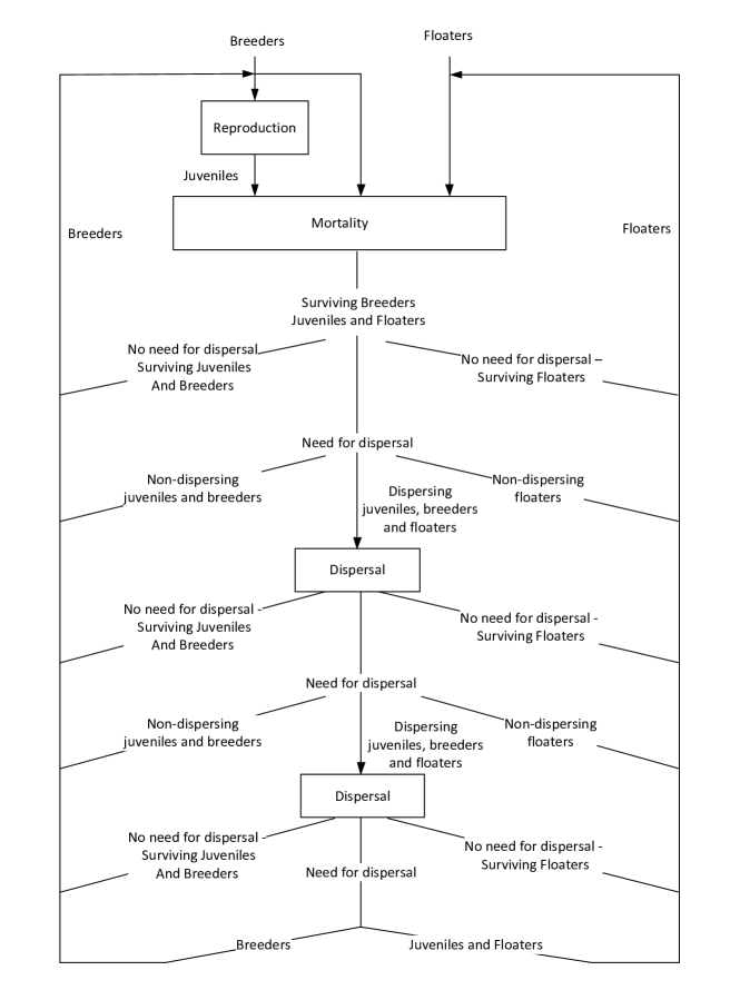
Figure 2: A cycle in the lifetime of the metapopulation

This metapopulation can be modeled in PALPS as follows. We consider the set of of locations and an associated predefined neighbor function as well as a distance function that may be instantiated according to the modeler’s preference to capture Euclidean distance or some other function of interest [27]. We also assume the existence of a set of probabilities $\{p_{i,j}\}_{i,j\in{\textbf{Loc}}}$ where $p_{i,j}$ represents the probability of dispersal from patch $i$ to patch $j$. Finally, we introduce the location attribute $c_{\ell}$ as a measure of the capacity of patch $\ell$. Then, wood thrush species can be modeled by the process $R=!rep.Juv$, where the behavior of a juvenile individual $J_{i}$ is described by the following equations:

$Juv$	$\stackrel{{\scriptstyle{\rm def}}}{{=}}$	$q_{j}:JC_{0}+(1-q_{j}):{\bf 0}$	Juvenile survival
$JC_{0}$	$\stackrel{{\scriptstyle{\rm def}}}{{=}}$	${\sf cond}\;(@{\sf myloc}>c_{{\sf myloc}}\rhd JD_{0},{\sf true}\rhd\surd.AB)$	Check patch capacity
$JD_{0}$	$\stackrel{{\scriptstyle{\rm def}}}{{=}}$	$p_{j}:JA_{1}+(1-p_{j}):\surd.AB$	Decide whether to disperse
$JA_{1}$	$\stackrel{{\scriptstyle{\rm def}}}{{=}}$	$\sum_{\ell\in Neigh({\sf myloc})}p_{{\sf myloc},\ell}:go\,\ell.JC_{1}$	Dispersal attempt $1$
$JC_{1}$	$\stackrel{{\scriptstyle{\rm def}}}{{=}}$	${\sf cond}\;(@{\sf myloc}>c_{{\sf myloc}}\rhd JD_{1},{\sf true}\rhd\surd.AB)$	Check patch capacity
$JD_{1}$	$\stackrel{{\scriptstyle{\rm def}}}{{=}}$	$p_{j}:JA_{2}+(1-p_{j}):\surd.AB$	Decide whether to disperse
$JA_{2}$	$\stackrel{{\scriptstyle{\rm def}}}{{=}}$	$\sum_{\ell\in Neigh({\sf myloc})}p_{{\sf myloc},\ell}:go\,\ell.JC_{2}$	Dispersal attempt $2$
$JC_{2}$	$\stackrel{{\scriptstyle{\rm def}}}{{=}}$	${\sf cond}\;(@{\sf myloc}>c_{{\sf myloc}}\rhd\surd.Fl,{\sf true}\rhd\surd.AB)$	Become floater or adult
$AB$	$\stackrel{{\scriptstyle{\rm def}}}{{=}}$	$r_{b}:\overline{r_{b}}_{i}.BS+(1-rb):BS$	Breeder reproduction
$BS$	$\stackrel{{\scriptstyle{\rm def}}}{{=}}$	$q_{b}:BC_{0}+(1-q_{b}):{\bf 0}$	Breeder survival
$BC_{0}$	$\stackrel{{\scriptstyle{\rm def}}}{{=}}$	${\sf cond}\;(@{\sf myloc}>c_{{\sf myloc}}\rhd BD_{0},{\sf true}\rhd\surd.AB)$	Check patch capacity
$BD_{0}$	$\stackrel{{\scriptstyle{\rm def}}}{{=}}$	$p_{b}:BA_{1}+(1-p_{b}):\surd.AB$	Decide whether to disperse
$BA_{1}$	$\stackrel{{\scriptstyle{\rm def}}}{{=}}$	$\sum_{\ell\in Neigh({\sf myloc})}p_{{\sf myloc},\ell}:go\,\ell.BC_{1}$	Dispersal attempt $1$
$BC_{1}$	$\stackrel{{\scriptstyle{\rm def}}}{{=}}$	${\sf cond}\;(@{\sf myloc}>c_{{\sf myloc}}\rhd BD_{1},{\sf true}\rhd\surd.AB)$	Check patch capacity
$BD_{1}$	$\stackrel{{\scriptstyle{\rm def}}}{{=}}$	$p_{b}:BA_{2}+(1-p_{b}):\surd.AB$	Decide whether to disperse
$BA_{2}$	$\stackrel{{\scriptstyle{\rm def}}}{{=}}$	$\sum_{\ell\in Neigh({\sf myloc})}p_{{\sf myloc},\ell}:go\,\ell.BC_{2}$	Dispersal attempt $2$
$BC_{2}$	$\stackrel{{\scriptstyle{\rm def}}}{{=}}$	${\sf cond}\;(@{\sf myloc}>c_{{\sf myloc}}\rhd\surd.Fl,{\sf true}\rhd\surd.AB)$	Floater or adult
$Fl$	$\stackrel{{\scriptstyle{\rm def}}}{{=}}$	$q_{f}:FC_{0}+(1-q_{f}):{\bf 0}$	Floater survival
$FC_{0}$	$\stackrel{{\scriptstyle{\rm def}}}{{=}}$	${\sf cond}\;(@{\sf myloc}>c_{{\sf myloc}}\rhd FD_{0},{\sf true}\rhd\surd.Fl)$	Check patch capacity
$FD_{0}$	$\stackrel{{\scriptstyle{\rm def}}}{{=}}$	$p_{f}:FA_{1}+(1-p_{f}):\surd.Fl$	Decide whether to disperse
$FA_{1}$	$\stackrel{{\scriptstyle{\rm def}}}{{=}}$	$\sum_{\ell\in Neigh({\sf myloc})}p_{{\sf myloc},\ell}:go\,\ell.FC_{1}$	Dispersal attempt $1$
$FC_{1}$	$\stackrel{{\scriptstyle{\rm def}}}{{=}}$	${\sf cond}\;(@{\sf myloc}>c_{{\sf myloc}}\rhd FD_{1},{\sf true}\rhd\surd.Fl)$	Check patch capacity
$FD_{1}$	$\stackrel{{\scriptstyle{\rm def}}}{{=}}$	$p_{f}:FA_{2}+(1-p_{f}):\surd.Fl$	Decide whether to disperse
$FA_{2}$	$\stackrel{{\scriptstyle{\rm def}}}{{=}}$	$\sum_{\ell\in Neigh({\sf myloc})}p_{{\sf myloc},\ell}:go\,\ell.\surd.Fl$	Dispersal attempt $2$

As before, the system can be modeled as the composition of the species as well as the various individuals that form the study:

$$System\stackrel{{\scriptstyle{\rm def}}}{{=}}[(R{:}[\![{1}]\!]\mid\prod_{1\leq i\leq n_{b}^{1}}AB{:}[\![{\ell_{1},1}]\!]\mid\mid\prod_{1\leq i\leq n_{j}^{1}}Juv{:}[\![{\ell_{1},1}]\!]\mid\prod_{1\leq i\leq n_{f}^{1}}Fl{:}[\![{\ell_{1},1}]\!]\ldots)\backslash\{rep_{1},\ldots rep_{k}\}.$$

Varying the model parameters, e.g. the habitat topology, patch quality and dispersal distance, may allow an analysis of the effects of the parameters on patch and metapopulation persistence.

4 Concluding remarks

This paper reports on work towards the development of a process-calculus framework for the spatially-explicit and individual-based modeling of ecological systems. In related work [2] we have also implemented a prototype tool and conducted simulations for the spatially-explicit model of [9]. In future work we intend to provide optimizations for our tool via an implementation of a spatial extension of the Gillespie simulation algorithm [13, 22] and by taking advantage of concepts developed in process-algebraic frameworks for state-space reduction such as confluence and minimization according to equivalence relations. At the same time it is our intention to enhance the syntax of PALPS to enable a more succinct presentation of systems especially in terms of the multiplicity of individuals. Other possible directions for future work include the adoption of continuous time as well as the use of dynamic attributes to allow exploring the system while patch quality degrades, temperatures increase, etc.

References

- [1]
- [2] M. Antonaki (2012): A Probabilistic Process Algebra and a Simulator for Modeling Population Systems. Master’s thesis, University of Cyprus.
- [3] R. Barbuti, A. Maggiolo-Schettini, P. Milazzo & G. Pardini (2011): Spatial Calculus of Looping Sequences. Theoretical Computer Science 412(43), pp. 5976–6001, 10.1016/j.tcs.2011.01.020.
- [4] L. Berec (2002): Techniques of spatially explicit individual-based models: construction, simulation, and mean-field analysis. Ecological Modeling 150, pp. 55–81, 10.1016/S0304-3800(01)00463-X.
- [5] D. Besozzi, P. Cazzaniga, D. Pescini & G. Mauri (2008): Modelling metapopulations with stochastic membrane systems. BioSystems 91(3), pp. 499–514, 10.1016/j.biosystems.2006.12.011.
- [6] D. Besozzi, P. Cazzaniga, D. Pescini & G. Mauri (2010): An Analysis on the Influence of Network Topologies on Local and Global Dynamics of Metapopulation Systems. In: Proceedings of AMCA-POP’10, pp. 1–17, 10.4204/EPTCS.33.1.
- [7] A. Bianco & L. de Alfaro (1995): Model checking of probabilistic and nondeterministic systems. In: Proceedings of FSTTCS’95, LNCS 1026, Springer, pp. 499–513, 10.1007/3-540-60692-0_70.
- [8] L. Bioglio, C. Calcagno, M. Coppo, F. Damiani, E. Sciacca, S. Spinella & A. Troina (2011): A Spatial Calculus of Wrapped Compartments. CoRR abs/1108.3426. Available at http://arxiv.org/abs/1108.3426.
- [9] A. Brännström & D. J. T. Sumpter (2005): Coupled map lattice approximations for spatially explicit individual-based models of ecology. Bulletin of Mathematical Biology 67(4), pp. 663–682, 10.1016/j.bulm.2004.09.006.
- [10] L. Cardelli (2005): Brane Calculi - Interactions of Biological Membranes. In: Proceedings of CMSB’04, LNCS 3082, Springer, pp. 257 –278, 10.1007/978-3-540-25974-9_24.
- [11] L. Cardelli & P. Gardner (2010): Processes in space. In: Proceedings of CiE 2010, LNCS 6158, Springer, pp. 78–87, 10.1007/978-3-642-13962-8_9.
- [12] M. Cardona, M. Colomer, A. Margalida, I. Pérez-Hurtado, M. J. Pérez-Jiménez & D. Sanuy (2009): A P System Based Model of an Ecosystem of the Scavenger Birds. In: Proceedings of WMC’09, LNCS 5957, Springer, pp. 182–195, 10.1007/978-3-642-11467-0_14.
- [13] P. Cazzaniga, D. Pescini, D. Besozzi & G. Mauri (2006): Tau Leaping Stochastic Simulation Method in P Systems. In: Proceedings of WMC’06, LNCS 4361, Springer, pp. 298–313, 10.1007/11963516_19.
- [14] F. Ciocchetta & M. L. Guerriero (2009): Modelling biological compartments in Bio-PEPA. Electronic Notes in Theoretical Computer Science 227, pp. 77–95, 10.1016/j.entcs.2008.12.105.
- [15] F. Ciocchetta & J. Hillston (2009): Bio-PEPA: a Framework for the Modelling and Analysis of Biochemical Networks. Theoretical Computer Science 410(33-34), pp. 3065–3084, 10.1016/j.tcs.2009.02.037.
- [16] J. B. Dunning, D. J. Stewart, B. J. Danielson, B. R. Noon, T. L. Root, R. H. Lamberson & E. E. Stevens (1995): Spatially Explicit Population Models: Current Forms and Future Uses. Ecological Applications 5, pp. 3–11, 10.2307/1942045.
- [17] V. Forejt, M. Kwiatkowska, G. Norman & D. Parker (2011): Automated Verification Techniques for Probabilistic Systems. In: Proceedings of SFM’11, LNCS 6659, Springer, pp. 53–113, 10.1007/978-3-642-21455-4_3.
- [18] S. C. Fu & G. Milne (2004): A Flexible Automata Model for Disease Simulation. In: Proceedings of ACRI’04, LNCS 3305, Springer, pp. 642–649, 10.1007/978-3-540-30479-1_66.
- [19] V. Galpin (2009): Modelling Network Performance with a Spatial Stochastic Process Algebra. In: Proceedings of AINA’09, IEEE Computer Society, pp. 41–49, 10.1109/AINA.2009.75.
- [20] L. R. Gerber & G. R. VanBlaricom (2001): Implications of three viability models for the conservation status of the western population of Steller sea lions (Eumetopias jubatus). Biological Conservation 102, pp. 261– 269, 10.1016/S0006-3207(01)00104-5.
- [21] C. A. R. Hoare (1985): Communicating Sequential Processes. Prentice-Hall.
- [22] M. Jeschke, R. Ewald & A. Uhrmacher (2011): Exploring the performance of spatial stochastic simulation algorithms. Journal of Computational Physics 230(7), pp. 2562–2574, 10.1016/j.jcp.2010.12.030.
- [23] M. John, R. Ewalda & A. M. Uhrmacher (2008): A Spatial Extension to the -Calculus. Electronic Notes in Theoretical Computer Science 194, pp. 133–148, 10.1016/j.entcs.2007.12.010.
- [24] D. Kouzapas & A. Philippou (2011): A Process Calculus for Dynamic Networks. In: Proceedings of FMOODS/FORTE’11, LNCS 6722, Springer, pp. 213–227, 10.1007/978-3-642-21461-5_14.
- [25] C. McCaig, R. Norman & C. Shankland (2008): Process Algebra Models of Population Dynamics. In: Proceedings of AB’08, LNCS 5147, Springer, pp. 139–155, 10.1007/978-3-540-85101-1_11.
- [26] R. Milner (1980): A Calculus of Communicating Systems. Springer.
- [27] E. S. Minor, R. I. McDonald, E. A. Treml & D. L. Urban (2008): Uncertainty in spatially explicit population models. Biological Conservation 141(4), pp. 956–970, 10.1016/j.biocon.2007.12.032.
- [28] G. Pardini (2011): Formal Modelling and Simulation of Biological Systems with Spatiality. Ph.D. thesis, University of Pisa.
- [29] R. G. Pearson & T. P. Dawson (2005): Long-distance plant dispersal and habitat fragmentation: identifying conservation targets for spatial landscape planning under climate change. Biological Conservation 123, pp. 389–401, 10.1016/j.biocon.2004.12.006.
- [30] G. Păun (2002): Membrane Computing: An Introduction. Springer-Verlag.
- [31] A. Regev, E. M. Panina, W. Silverman, L. Cardelli & E. Shapiro (2004): BioAmbients: an Abstraction for Biological Compartments. Theoretical Computer Science 325(1), pp. 141–167, 10.1016/j.tcs.2004.03.061.
- [32] C. Tofts (1994): Processes with probabilities, priority and time. Formal Aspects of Computing 6, pp. 536–564, 10.1007/BF01211867.
- [33] J. M. J. Travis & C. Dytham (1998): The evolution of disperal in a metapopulation: a spatially explicit, individual-based model. Proceedings: Biological Sciences 265(1390), pp. 17–23, 10.1098/rspb.1998.0258.
- [34] D. L. Urban & H. H. Shugart (1986): Avian demography in mosaic landscapes: modeling paradigm and preliminary results. Wildlife 2000: Modeling Habitat Relationships of Terrestrial Vertebrates, pp. 273–279.