Stochastic accretion and the variability of supergiant fast X–ray transients

Abstract

In this paper we consider the variability of the luminosity of a compact object (CO) powered by the accretion of an extremely inhomogeneous (“clumpy”) stream of matter. The accretion of a single clump results in an X-ray flare: we adopt a simple model for the response of the CO to the accretion of a single clump, and derive a stochastic differential equation (SDE) for the accretion powered luminosity $L(t)$. We put the SDE in the equivalent form of an equation for the flares’ luminosity distribution (FLD), and discuss its solution in the stationary case.

As a case study, we apply our formalism to the analysis of the FLDs of Super-Giant Fast X-ray Transients (SFXTs), a peculiar sub-class of High Mass X–ray Binary Systems (HMXBs). We compare our theoretical FLDs to the distributions observed in the SFXTs $IGR\leavevmode\nobreak\ J16479-4514$, $IGR\leavevmode\nobreak\ J17544-2619$ and $XTE\leavevmode\nobreak\ J1739-302$.

Despite its simplicity, our model fairly agrees with the observed distributions, and allows to predict some properties of the stellar wind. Finally, we discuss how our model may explain the difference between the broad FLD of SFXTs and the much narrower distribution of persistent HMXBs.

1 Introduction

In several astrophysical contexts the mass accretion onto a compact object (CO, a black hole, a neutron star a or white dwarf) cannot be considered as a continuous process. The accretion may be discrete: the mass does not flow as a continuous stream, but consists of a volley of clumps whose accretion on the compact object results in a flaring activity observed in the X–ray/$\gamma$ ray spectral window. Inhomogeneous flows occur in the Polar (a.k.a. AM Herculis) cataclysmic variables (e.g. Warner, 1995), or in the Supergiant Fast X–ray Transients (Sguera et al., 2006, Negueruela et al., 2006; in’t Zand, 2005). Understanding the properties of clumpy accretion on the super–massive black holes hosted at the core of galaxy clusters is also relevant in the context of the “cold feedback model” (e.g. Pizzolato and Soker, 2005).

The luminosity $L(t)$ powered by the accretion on a compact object results from the interplay of two factors: the properties of the accreting stream and the response of the CO to their arrival. The response process may be quite complex, but it is essentially deterministic. On the other hand, if the accretion occurs from a population of clumps with random masses arriving at random times, the accretion driving term is a stochastic process. The accretion-powered luminosity $L(t)$ is an irregular function of time, and it requires an adequate mathematical tool to be dealt with. This is provided by the theory of stochastic differential equations (SDEs), that replaces the rules of ordinary calculus to treat highly irregular functions (see e.g. Øksendal, 2003; Gardiner, 2009).

In this paper we consider the variability of the X/$\gamma$ ray luminosity of a CO powered by the accretion of a family of clumps with randomly distributed masses. We shall derive (Sec. 2) a simple SDE for the luminosity $L(t)$, and will illustrate some of the subtleties involved in handling SDEs. A possible way to use this SDE is to compute a sample path of $L(t)$, to be compared to an observed light curve. An equivalent approach (presented in Sec. 3) consists in associating to the SDE for $L(t)$ an integro-differential equation (known as “generalised Fokker-Planck equation”, GFPE) for the probability function $p(L,t)$ that the source has luminosity $L$ at the time $t$. We shall discuss the properties of the distribution $p$, and how it mirrors the features of the accreting stream. As a case study we apply our model to the super-giant Fast X–ray Transients (SFXTs), an interesting class of High Mass X–ray binaries composed by a neutron star (or a black hole) accreting an extremely inhomogeneous wind blown by its massive companion. Our analysis of SFXTs is presented in Sec. 4. We shall discuss our findings and in particular how our model helps to explain the difference of the FLDs of SFXTs from those of the much more common persistent X-ray sources. We shall summarise in Sec. 5.

2 A simple stochastic accretion model

The analysis of the long term variability of the X–ray light curve generated by the inhomogeneous accretion requires some modelling of the response of the CO the the accretion process of a single clump. To this purpose it is helpful to imagine the CO as a “black box” that emits X–rays in response to the accretion of mass from the surrounding environment. If ${\dot{M}}_{c}$ is the mass capture rate and $L$ is the luminosity produced by the CO, we postulate the linear response

$$L(t)=\int_{\mathbb{R}}dt^{\prime}\;W(\mathbf{p},t-t^{\prime})\>{\dot{M}}_{c}(t^{\prime}),$$ (1)

where the function $W$ (dependent on the parameters $\mathbf{p}$) describes the response of the CO.

The analytical shape of $W$ may be exceedingly complex, since it must embody a number of physical processes: tidal effects, interaction of the accretion flow with the magnetic field of the CO, geometry and plasma instabilities of the accretion stream, radiation effects, and so on. Since this paper aims to focus on the basic properties of the accretion process, we steer clear of these details and demand for $W$ just few very basic properties; i) $W(t)$ is causal: it vanishes for $t<0$, i.e. before the capture of a clump, and ii) it decays to zero for $t\gg 0$, i.e. long after the clump has been captured. The simplest function with these properties is

$${W}(t)=\left\{\begin{aligned} &0&t<0\\ &\frac{G\,M}{{R_{\rm st}}}\;\frac{{\rm e}^{-t/\tau}}{\tau}&t\geq 0\end{aligned}\right..$$ (2)

This response gives the accretion powered luminosity of a unit mass on a CO of mass $M$, down to a “stopping radius” ${R_{\rm st}}$. If the CO is able to accrete the flow down to its radius (or event horizon) $R$, then ${R_{\rm st}}=R$. In some cases, e.g. a fast spinning magnetised neutron star, the so called “propeller” effect (see e.g. Lipunov, 1987; Illarionov and Sunyaev, 1975; Davies et al., 1979; Davies and Pringle, 1981) prevents the stream to flow beyond the magnetosphere, and in this case ${R_{\rm st}}$ is the Alfvén radius $R_{A}$. The time scale $\tau$ represents the time scale taken by the CO to “process” the accretion stream. For example, if the stream has an appreciable angular momentum, it forms an accretion disc before falling on the CO, and the mass accretion rate on the CO decays as a power law on the viscous time scale

$$\tau\simeq 7.5\times 10^{5}\leavevmode\nobreak\ {\rm s}\;\alpha^{-4/5}\>\left(\frac{{\dot{M}}}{10^{-11}{\leavevmode\nobreak\ M_{\odot}\,\rm yr^{-1}}}\right)^{-3/10}\;{\left(\frac{M_{\rm ns}}{1.4\leavevmode\nobreak\ M_{\odot}}\right)}^{1/4}\;\left(\frac{R_{\rm out}}{10^{10}{\leavevmode\nobreak\ \rm cm}}\right)^{5/4},$$ (3)

(Eq. 5.63 in Frank et al., 2002), where $R_{\rm out}$ is the outer radius and $\alpha\lesssim 1$ is the viscosity parameter (Shakura and Sunyaev, 1973).

It is instructive to consider Eqns. (1) and (2) in the simple case of the accretion a single clump of mass $m$, with ${\dot{M}}_{c}(t)=m\,\delta(t)$ (where $\delta$ is the Dirac delta function). With our choice (2) of the response $W$, the luminosity is zero at $t<0$, i.e. before the clumps arrives, and

$$L=\frac{G\,M}{R_{\rm st}}\>\frac{m}{\tau}\;{\rm e}^{-t/\tau}$$ (4)

for $t\geq 0$. The luminosity has a sharp peak, and then decays exponentially with the e-folding time $\tau$. Plugging the Ansatz (2) into Eq. (1) we find

$$\tau\>\frac{d\,{L}}{d\,{t}}=\frac{G\,M}{R_{\rm st}}\;{\dot{M}}_{c}-L.$$ (5)

We introduce the mass accretion rate ${\dot{M}}$ accreted down to the stopping radius ${R_{\rm st}}$

$$L\equiv\frac{G\,M}{{R_{\rm st}}}\>{\dot{M}},$$ (6)

so Eq. (5) becomes

$$\tau\>\frac{d\,{{\dot{M}}}}{d\,{t}}={\dot{M}}_{c}-{\dot{M}}.$$ (7)

Since the function ${\dot{M}}_{c}(t)$ is random, the function ${\dot{M}}(t)$ is highly irregular and certainly not differentiable, so Eq. (7) is to be interpreted as a stochastic differential equation (see e.g. Øksendal, 2003), and not as an ordinary differential equation.

Thus far we have provided a simple model for the “response” of the compact object to the accretion of a clump of matter. We now turn our attention to the driving stochastic term ${\dot{M}}_{c}$, which embodies both the arrival rate of the clumps and their mass distribution. Neglecting the finite size of the clumps, we model the clumps’ arrival rate as a train of delta pulses

$${\dot{M}}_{c}(t)=\sum_{k=1}^{n(t)}m_{k}\>\delta(t-t_{k}),$$ (8)

where $m_{k}$ is the mass of the clump accreted at the time $t_{k}$, and $n(t)$ is a Poisson counting process, described by the probability

$${\mathcal{P}}[n(t)=n]=\frac{{\rm e}^{-\lambda\,t}\,(\lambda\,t)^{n}}{n!},$$ (9)

where $\lambda$ is the clumps’ arrival rate. The masses $\{m_{k}\}$ are distributed according to the probability distribution function $\varphi(m)$; we assume that $\varphi$ is stationary, and that the random variables $\{m_{k}\}$ and $\{t_{k}\}$ are uncorrelated. The statistical properties of ${\dot{M}}_{c}$ are readily derived:

$${\langle{{\dot{M}}_{c}}\rangle} =\lambda\;{\langle{m}\rangle}$$ (10a)

$${\langle{{\dot{M}}_{c}(t)\>{\dot{M}}_{c}(t^{\prime})}\rangle} =\lambda\;{\langle{m^{2}}\rangle}\;\delta(t-t^{\prime}).$$ (10b)

The properties (10) show that the Poisson process (8) is a white noise with non–zero mean.

From Eqns. (7), (8) and (10) it is possible to derive some properties of the random function ${\dot{M}}(t)$. They not only provide a useful check against our more elaborate approach developed in the next sections, but they also help to point out some subtle key properties of SDEs.

Integrating Eq. (7), we find the expression

$$\tau\,d{\dot{M}}=\delta m(t)-{\dot{M}}(t)\,dt,$$ (11)

where

$$\delta m(t)=\int_{t}^{t+d\,t}dt^{\prime}{\dot{M}}_{c}(t^{\prime}).$$ (12)

With the aid of Eqns. (10) we derive

$${\langle{\delta m}\rangle}=\int_{t}^{t+dt}dt^{\prime}{\langle{{\dot{M}}_{c}(t^{\prime})}\rangle}=\lambda\ {\langle{m}\rangle}\,dt$$ (13a)

$${\langle{(\delta m)^{2}}\rangle}=\int_{t}^{t+dt}dt^{\prime}\int_{t}^{t+dt}dt^{\prime\prime}{\langle{{\dot{M}}_{c}(t^{\prime}){\dot{M}}_{c}(t^{\prime\prime})}\rangle}=\lambda\ {\langle{m^{2}}\rangle}\,dt.$$ (13b)

With the first of these expressions we find the mean of Eq. (11), i.e. the ordinary differential equation

$$\tau\,\frac{d\,{{\langle{{\dot{M}}}\rangle}}}{d\,{t}}=\lambda\,{\langle{m}\rangle}-{\langle{{\dot{M}}}\rangle}$$ (14)

(the order of the mean and the derivative may be exchanged, see e.g. Reif, 1965).

For $t\gg\tau$ the mean mass accretion rate ${\langle{{\dot{M}}}\rangle}$ relaxes on the stationary value

$${\langle{{\dot{M}}}\rangle}=\lambda\,{\langle{m}\rangle}.$$ (15)

The evaluation of the second moment is trickier, on account of the stochastic nature of the equation. We write

$$\tau\,d({\dot{M}}^{2})=\tau\left[({\dot{M}}+d\,{\dot{M}})^{2}-{\dot{M}}^{2}\right]=\tau\,\left[2{\dot{M}}d{\dot{M}}+(d{\dot{M}})^{2}\right],$$ (16)

where in the expansion we must keep the second order term $(d{\dot{M}})^{2}$ for reason that will be clear soon. Plugging Eq. (11) into this expression we get

$$\tau\,d({\dot{M}}^{2})=2\,{\dot{M}}\left(\delta m-{\dot{M}}(t)\,dt\right)+(\delta m)^{2}+O(dt),$$ (17)

and taking the mean by using Eqns. (13) we find the ordinary differential equation

$$\tau\,\frac{d\,{{\langle{{\dot{M}}^{2}}\rangle}}}{d\,{t}}=2\lambda^{2}{\langle{m}\rangle}^{2}-2\,{\langle{{\dot{M}}^{2}}\rangle}+\frac{\lambda}{\tau}\,{\langle{m^{2}}\rangle}.$$ (18)

For $t\gg\tau$ the second moment ${\langle{{\dot{M}}^{2}}\rangle}$ relaxes on the stationary value

$${\langle{{\dot{M}}^{2}}\rangle}=\lambda^{2}{\langle{m}\rangle}^{2}+\frac{\lambda}{2\,\tau}{\langle{m^{2}}\rangle},$$ (19)

corresponding to the variance

$$\sigma_{{\dot{M}}}^{2}={\langle{{\dot{M}}^{2}}\rangle}-{\langle{{\dot{M}}}\rangle}^{2}=\frac{\lambda}{2\,\tau}{\langle{m^{2}}\rangle}.$$ (20)

Some remarks are in order. First, the stochastic nature of the function ${\dot{M}}_{c}$ makes ${\dot{M}}(t)$ an extremely irregular function of time. On account of such irregular behaviour, none of the rules of ordinary calculus are applicable to ${\dot{M}}(t)$. One consequence is that the second order differential $(d{\dot{M}})^{2}$ is proportional to $dt$, and therefore it cannot be neglected in the formal manipulations, as we have done in Eq. (16). In order to work with such irregular functions a new kind of differential calculus (known as “Itō calculus”) has been developed as a corner stone of the theory of stochastic differential equations (SDEs, see e.g. Øksendal, 2003). Some level of knowledge of SDEs is therefore essential to master the modelling of random processes like that studied in this paper.

The moments ${\langle{{\dot{M}}^{n}}\rangle}$ exist only if the correspondent moments ${\langle{m^{n}}\rangle}$ of the clumps’ distribution are defined. This is not always the case, e.g. when the distribution $\varphi$ has a fat tail. In order to deal with such possibility, it is necessary to extend the simple approach presented in this section. We shall explain how in Sec. 2.1.

The mean accretion rate (15) depends on the clumps’ arrival rate $\lambda$, but not from the relaxation time $\tau$, which is an intrinsic property of the accretor. The variance (20) features the relaxation time $\tau$ with an inverse power: a long relaxation time $\tau$ corresponds to a narrow dispersion of the observed values of ${\dot{M}}$ around the mean. Indeed, if the relaxation time $\tau$ is long, several clumps may be accreted before the accretor is able to respond, and an observer cannot distinguish between several elementary accretion processes, which are perceived as a single accretion of a large clump. Clearly, this has the effect of reducing the dispersion of the observed distribution.

2.1 Direct SDE vs Fokker-Planck approach

In principle, Eq. (7) may be solved numerically. Several computing techniques have been developed to tackle the numerical solution of SDEs (see e.g. Kloeden and Platen, 1999). A sample of the population of the clumps’ masses and arrival times are extracted from the distributions $\varphi$ and ${\mathcal{P}}[n(t)]$ (defined by Eq. (9)). A sample path of the process ${\dot{M}}(t)$ is computed numerically, and ${\dot{M}}(t)$ is converted to the accretion luminosity $L(t)$ via Eq. (6). A sample path $L_{1}(t)$ may be very different from another path $L_{2}(t)$, since the clumps’ masses and arrival times extracted from the distributions $\varphi$ and ${\mathcal{P}}[n(t)]$ used to compute $L_{1}(t)$ numerically may be very different from those extracted to compute $L_{2}(t)$. For this reason, it is meaningless to compare a single sample path of $L(t)$ with a real light curve. Any comparison of a stochastic model with the observations will involve some statistics on a sample of the computed paths and the light curves.

We shall adopt an equivalent approach to achieve the goal of comparing a theoretical stochastic light curve with a real light curve. It is possible to associate to Eq. (7) a new equation (called a “generalised Fokker–Planck equation”, GFPE) for the probability $p(L,t)$ that the source has luminosity $L$ at the time $t$. The distribution $p$ is directly comparable to the histogram of the flares’ luminosities observed in a real source over a long time span.

The approach based on the luminosity distribution $p(L,t)$ allows to deal quite straightforwardly with a complication we have overlooked thus far. The luminosity distribution is defined as a function of the X–ray luminosity $L$, not of the mass accretion rate ${\dot{M}}$. The general relation between the luminosity distribution $p(L,t)$ and the mass accretion rate distribution $P({\dot{M}},t)$ is

$$p(L,t)=\left|\frac{d\,{{\dot{M}}}}{d\,{L}}\right|\>P({\dot{M}},t)$$ (21)

If all the mass can reach the surface of the neutron star (located at the radius $R$), then $R_{\rm st}=R$. In this case the distributions $p(L)$ and $P({\dot{M}})$ are simply proportional to each other:

$$p(L,t)=\frac{R}{G\,M}\;P({\dot{M}},t).$$ (22)

In some systems, however, the accreting stream cannot reach the surface: this is typically the case of a magnetised fast spinning neutron star in which the matter is captured by the star’s gravitational field, but is prevented from reaching its surface by a “propeller” barrier. At a very basic level, the “propeller” effect may be described as follows. The matter inside the magnetosphere (located at the Alfvén radius $R_{A}$) is forced to rotate with the same angular velocity $\omega_{\rm ns}$ as the neutron star. On the other hand, the angular velocity of the mass stream outside the magnetosphere ($r>R_{A}$) is approximately keplerian, $\omega\simeq\omega_{K}(r)$. If

$$\omega_{\rm ns}>\omega_{K}(R_{A})$$ (23)

no accretion is possible, and the matter is stopped at the Alfvén radius. The radius $R_{A}$ depends on the geometry of the accretion flow. If NS accretes a clumpy wind in a detached binary system the accretion is approximately spherical, and there are two possible regimes. The NS crosses a wind blown by the companion star with a velocity $v_{w}$. This wind is focused by the NS’s own gravitational field within the capture radius

$$R_{G}=\frac{2\,G\,{M_{\rm ns}}}{v_{w}^{2}}=3.74\times 10^{10}{\leavevmode\nobreak\ \rm cm}\;{\left(\frac{M_{\rm ns}}{1.4\leavevmode\nobreak\ M_{\odot}}\right)}\;\left(\frac{v_{w}}{10^{3}{\leavevmode\nobreak\ \rm km\,s^{-1}}}\right)^{-2}.$$ (24)

If the magnetic field of the NS is “weak”, then the wind is first focused by the NS’s gravitational field, and only then it is affected by the NS’ magnetic force. In this case the correct expression of the Alfvén radius is (e.g. Lipunov, 1987)

$$R_{A}=\left(\frac{\mu^{4}}{2\,G\,{M_{\rm ns}}\,{\dot{M}}^{2}}\right)^{1/7}\qquad\text{if}\qquad R_{A}<R_{G},$$ (25)

where $\mu$ is the magnetic moment of the NS. On the other hand, if the magnetic field is strong, then the wind feels NS’ magnetic field before its gravity, and in this regime

$$R_{A}=\left(\frac{4\,\mu^{2}G^{2}\,{M_{\rm ns}}^{2}}{{\dot{M}}\,v_{w}^{5}}\right)^{1/6}\qquad\text{if}\qquad R_{G}<R_{A}.$$ (26)

The critical mass accretion rate ${\dot{M}}_{\omega}$ at which the propeller barrier sets in can be derived from Eq. (23) with $R_{A}$ given by either Eq. (25) or Eq. (26). If ${\dot{M}}<{\dot{M}}_{\omega}$ the ram pressure exerted by the flow is unable to overcome the magnetic pressure at the magnetospheric radius, and the flow is stopped at the Alfvén radius $R_{A}$. The stopping radius is then

$${R_{\rm st}}=\left\{\begin{aligned} &R&{\dot{M}}>{\dot{M}}_{\omega}\\ &R_{A}&{\dot{M}}<{\dot{M}}_{\omega}\end{aligned}\right..$$ (27)

Plugging this stepwise function ${R_{\rm st}}({\dot{M}})$ into Eq. (21) we find

$$p(L,t)=\left\{\begin{aligned} &\frac{R_{A}}{G\,M}\;P({\dot{M}},t)&L<L_{1}\\ &0&L_{1}<L<L_{\omega}\\ &\frac{R}{G\,M}\;P({\dot{M}},t)&L>L_{\omega}\end{aligned}\right.,$$ (28)

where $L_{1}=G\,M{\dot{M}}_{\omega}/R_{A}$ and $L_{\omega}=G\,M\,{\dot{M}}_{\omega}/R$.

For a typical parameters of a NS ($\mu\simeq 10^{30}\leavevmode\nobreak\ \rm G$) and of a stellar wind ($v_{w}\simeq 10^{3}{\leavevmode\nobreak\ \rm km\,s^{-1}}$) the luminosity $L_{1}$ is below $\sim 10^{32}{\leavevmode\nobreak\ \rm erg\,s^{-1}}$, which is barely observable. Therefore, we neglect the tail below $L_{1}$ and approximate Eq. (28) with

$$p(L,t)\simeq\left\{\begin{aligned} &0&{\dot{M}}<{\dot{M}}_{\omega}\\ &\frac{R}{G\,M}\;P({\dot{M}},t)&{\dot{M}}>{\dot{M}}_{\omega}\end{aligned}\right..$$ (29)

In presence of an accretion barrier the luminosity distribution $p(L)$ has a sharp lower cut–off at the luminosity $L_{\omega}$.

Whether an accretion barrier is present or not, $p$ must be computed from the mass accretion distribution $P({\dot{M}},t)$. If no accretion barrier is present, $p$ is given by $P({\dot{M}},t)$ and Eq (22), else it is computed from $P({\dot{M}},t)$ and Eq. (29).

In the next section we derive and discuss the GFPE for $P({\dot{M}},t)$ associated to the stochastic differential equation (7).

3 The generalized Fokker–Planck equation

The method to derive the GFPE from a stochastic differential equation is described by Denisov et al. (2009). We leave all the technical details of the derivation in Appendix A, and here we reproduce only the results derived there. The GFPE associated to Eq. (7) reads

$$\tau\,\frac{\partial{P}}{\partial{t}}=\frac{\partial{\,({\dot{M}}\>P)}}{\partial{{\dot{M}}}}-\rho\>P({\dot{M}},t)+\rho\,\int_{0}^{\tau\,{\dot{M}}}d\,m\>\varphi(m)\;P\left({\dot{M}}-m/\tau,t\right),$$ (30a)

where

$$\rho=\lambda\,\tau$$ (30b)

is the accretion parameter. The solution of this equation is unique once we impose the normalisation

$$\int_{0}^{\infty}d{\dot{M}}\,P({\dot{M}},t)=1$$ (31)

and a suitable the initial condition.

A dimensional analysis (e.g. Barenblatt, 1996) helps to write Eq. (30a) in non-dimensional form. Suppose that $\varphi$ depends on the characteristic mass $m_{0}$ as the only dimensional parameter. The only dimensional parameters in the distribution $P$ are then ${\dot{M}}$, $t$, $\tau$ and $m_{0}$. Note that the clumps’ arrival rate $\lambda$ appears in the equation only in the dimensionless combination $\rho=\lambda\,\tau$, and therefore it does not appear as a separate variable. The only way to combine the governing dimensional variables into dimensionless variables (from which $P$ must depend) are

$$x={\dot{M}}\,\tau/m_{0}\qquad s=t/\tau.$$ (32)

so

$$P=P\left(\frac{{\dot{M}}\,\tau}{m_{0}},t/\tau\right)$$ (33)

(we do not indicate the dependence on possible other dimensionless parameters). Plugging this expression into Eq. (30a) we retrieve

$$\frac{\partial{\tilde{P}}}{\partial{s}}=x\,\frac{\partial{\tilde{P}}}{\partial{x}}+(1-\rho)\>\tilde{P}+\rho\,\int_{0}^{x}d\,y\>\tilde{\varphi}(x-y)\;\tilde{P}\left(y,s\right),$$ (34)

where $\tilde{P}=P\,m_{0}/\tau$ and $\tilde{\varphi}=\varphi\,m_{0}$ are the scaled distributions $P$ and $\varphi$. In the following we shall refer to the dimensionless Eq. (34), omitting the tildes on the scaled quantities.

The problem (30) depends on some initial condition. After a long time $t\gg\tau$ the compact star has gathered a large sample of clumps, and the probability $P$ is expected to relax on an equilibrium, time independent configuration. In the remainder of this paper we will shall assume that that such an equilibrium has been achieved, and we will work with the stationary distribution, solution of

$$x\,\frac{d\,{P}}{d\,{x}}=(\rho-1)\,P-\rho\,\int_{0}^{x}dy\>\varphi(x-y)\;P\left(y\right),$$ (35a)

This is a Volterra integro-differential equation of the second kind, whose solution is unique once we impose the normalisation

$$\int_{0}^{\infty}dx\,P(x)=1.$$ (35b)

The solution to the problem (35) is particularly convenient via a Fourier (or Laplace) transform. This not only allows a numerical solution, but also yields some exact results on the moments of the distribution.

3.1 Solutions to the generalised Fokker–Planck Equation

In this section we derive a solution to the generalised Fokker–Planck equation. Although an exact solution does not exists for a general form of $\varphi$, the Fourier transform of $P$ is analytical. This allows to compute all the moments of $P$ as function of the moments of $\varphi$ (when they exist), and it is makes possible to compute numerically $P(x)$ by evaluating a Fourier integral.

The logarithm of the Fourier transform of Eq. (35a) reads

$$\ln P_{k}=-\rho\,\int_{0}^{k}\frac{dk^{\prime}}{k^{\prime}}\>(1-\varphi_{k^{\prime}}),$$ (36)

where $\varphi_{k}$ is the Fourier transform of $\varphi$, and where we have introduced the normalisation (35b) as $\ln P_{k=0}=0$. Plugging $\varphi_{k}$ into the last equation,

$$\ln P_{k}=\rho\,\int_{0}^{\infty}dy\>\varphi(y)\>{\rm Ein}(i\,k\,y),$$ (37)

being

$${\rm Ein}(\zeta)=\int_{0}^{\zeta}ds\>\frac{1-{\rm e}^{-s}}{s}$$ (38)

the entire exponential integral (see e.g. Abramowitz and Stegun, 1972). The inverse Fourier transform

$$P(x)=\int_{\mathbb{R}}\frac{d\,k}{2\,\pi}\>\exp\left[-i\,k\,x+\ln P_{k}\right],$$ (39)

is rather involved, and cannot be further simplified for a general $\varphi$. Yet, it is possible to derive some exact results. The function $\ln P_{k}$ is the cumulant distribution function (CDF) of $P(x)$. We Taylor-expand the entire exponential integral in Eq. (37) and compare the resulting expression with the definition of CDF

$$\ln P_{k}\equiv\sum_{r=1}^{\infty}\;\frac{(i\,k)^{r}\langle\langle x_{r}\rangle\rangle}{r!}$$ (40)

to obtain the cumulants

$$\langle\langle x_{r}\rangle\rangle=\rho\;{\langle{x^{r}}\rangle}/r,$$ (41)

or, in dimensional units,

$$\langle\langle{\dot{M}}_{r}\rangle\rangle=\frac{\rho}{r}\;\frac{{\langle{m^{r}}\rangle}}{\tau^{r}}.$$ (42)

From the cumulants it is easy to retrieve the first moments of the distribution $P$: in dimensional variables

$${\langle{{\dot{M}}}\rangle} =\lambda\;{\langle{m}\rangle}$$ (43a)

$$\sigma_{{\dot{M}}}^{2} =\frac{\lambda}{2\,\tau}\>{\langle{m^{2}}\rangle}$$ (43b)

$$\gamma_{1} =\frac{2\sqrt{2}}{3\,\rho^{1/2}}\;\frac{{\langle{m^{3}}\rangle}}{{\langle{m^{2}}\rangle}^{3/2}}$$ (43c)

$$\gamma_{2} =\frac{1}{\rho}\;\frac{{\langle{m^{4}}\rangle}}{{\langle{m^{2}}\rangle}^{2}},$$ (43d)

where ${\langle{{\dot{M}}}\rangle}$, $\sigma_{{\dot{M}}}^{2}$, $\gamma_{1}$ and $\gamma_{2}$ are respectively mean, variance, skewness and excess kurtosis of $P$ (see e.g. Sec. 14.1 of Press et al., 2007 for the definitions).

Mean and variance coincide with the values worked out in Sec. 2 from our simple analysis of Eq. (7). The higher order moments provide further qualitative details on the shape of the accretion distribution function $P$. The skewness $\gamma_{1}$ is always positive, meaning that $P$ has a long tail for large $x$. The kurtosis $\gamma_{2}$ is always positive as well, i.e. $P(x)$ is leptokurtic: it has a sharp peak and a heavy tail for large $x$. If the terms ${\langle{m^{n}}\rangle}$ are finite, the standardized moment of order $n$ of $P$ scales as $\rho^{1-n/2}$.

The computation of the Fourier integral (39) cannot be done analytically for any $\varphi$, but it can be tackled numerically. This will be done later for some choices of the distribution $\varphi$.

If $\varphi(m)$ is bounded for $m\to 0$, the asymptotic behaviour of $P$ for $x\ll 1$ is independent of $\varphi$. For small $x$ the integral in Eq. (35a) is negligible, and

$$P(x)\sim x^{\rho-1}\qquad\text{for}\qquad x\ll 1.$$ (44)

For small values of $x$, $P$ is suppressed if $\rho\gg 1$, and diverges for $\rho\leq 1$. This behaviour has a clear physical explanation. For simplicity, we assume that there is no accretion barrier, so $P$ may be read as a luminosity distribution. Consider the accretion of two small clumps, the second one hitting the system a time $\lambda^{-1}$ after the first one. The inequality $\rho<1$ means that the relaxation time $\tau$ is shorter than $\lambda^{-1}$: the compact object has time to process the first clump before the arrival of the second one, and their accretion triggers two successive flares. The accretion of each clump is “recorded” in the low luminosity tail, and therefore the value of $P$ may be high. On the other hand, if $\rho\gg 1$, the compact object cannot process the first clump before the arrival of the second one. The accretion of two closely separated clumps cannot trigger two different low luminosity flares. Such accretion episodes are “recorded” as the accretion of a singe larger clump, and the low luminosity tail of $P$ is depressed by this effect that for convenience will be referred to as “$\rho$ suppression”.

3.2 A Dirac delta mass clumps’ distribution

Before applying the present model to a concrete astrophysical problem, it is useful to sketch the properties of $P$ in the relatively simple case in which all the clumps have the same mass. The appropriate mass distribution is then (in dimensionless units)

$$\varphi(x)=\delta(x-1),$$ (45)

where $\delta$ is the Dirac delta function. The generalised Fokker–Planck equation (35a) reduces to the delay differential equation

$$x\,\frac{d\,{P}}{d\,{x}}=(\rho-1)\,P-\vartheta(x-1)\;P(x-1),$$ (46)

where $\vartheta(u)$ is the Heaviside step function, $\vartheta=0$ for $u<0$ and $\vartheta=1$ for $u>0$. The solution of Eq. (46) can be easily tackled numerically. Some plots of $P(x)$ are shown in Fig. 1 for several values of the accretion parameter $\rho$.

Figure 1: The accretion PDF for the delta clumps’ distribution (45) for several values of the accretion parameter $\rho$.

The mean of $P$ is ${\langle{x}\rangle}=\rho$ and the standard deviation is $\sigma=\sqrt{\rho/2}$. On account of the lack of massive clumps in the distribution (45) the distribution $P$ does not display a significant tail. If $\rho>1$, $P$ is also suppressed for $x\lesssim 1$. These effects make the distribution $P$ quite narrow around its mean. The limit distribution solution of (46) will be useful later as a benchmark for more complex cases.

3.3 A log-normal clumps’ mass distribution

We now explore in some detail the solution of the GFPE (30a) with a more general distribution of the clumps’ masses. To our purposes, it is particularly convenient to adopt the log-normal distribution

$$\varphi(x)=\frac{1}{x\,\sigma\,\sqrt{2\,\pi}}\;{\exp}\left[{-\frac{\ln^{2}x}{2\,\sigma^{2}}}\right],$$ (47)

defined for any $x>0$. This choice has several advantages. First, the log-normal is extremely flexible: by tuning the shape parameter $\sigma$, it may mimic distributions as different as a Dirac delta (for $\sigma\ll 1$), or a power law (for $\sigma\gtrsim 1$). The distribution (47) may be written (up to a constant factor) $\varphi\sim x^{-\zeta}$, where $\zeta=1+\ln x/2\,\sigma^{2}$. The exponent $\zeta$ is a slowly varying function of the range $x$, and for $x\ll{\rm e}^{{\sigma^{2}/2}}$ the log-normal $\varphi$ closely resembles a power law with index $\zeta\gtrsim 1$. All the moments of a log-normal are defined, being

$${\langle{x^{n}}\rangle}=\exp{\left(n^{2}\,\sigma^{2}/2\right)}.$$ (48)

Eqns. (43) and (48) give the moments of the distribution $P$

$${\langle{{\dot{M}}}\rangle} =\lambda\,m_{0}\;{\rm e}^{\sigma^{2}/2}$$ (49a)

$$\sigma_{{\dot{M}}}^{2} =\frac{\lambda}{2\,\tau}\;m_{0}^{2}\;{\rm e}^{2\,\sigma^{2}}$$ (49b)

$$\gamma_{1} =\frac{2\sqrt{2}}{3\,\rho^{1/2}}\;{\rm e}^{3\,\sigma^{2}/2}$$ (49c)

$$\gamma_{2} ={\rm e}^{4\,\sigma^{2}}/\rho.$$ (49d)

It is clear that the moments of $P$ are defined for any order $n$, but their magnitude rapidly increases with $n$ if $\sigma>1$, making $P$ heavy tailed.

The Fourier integral (39) cannot be computed exactly if $\varphi$ is a log-normal, but it must be evaluated numerically. The numerical calculation of Fourier integrals poses a well known problem, widely discussed in the mathematical literature. A very convenient numerical method is a variant of the double exponential quadrature (see e.g. Mori and Sugihara, 2001) suggested by Ooura and Mori (1999).

Figure 2: Two samples of theoretical curves computed from the log-normal distribution (47). In the top panel $\rho$ is fixed at $\rho=10$ and the curves refer at different values of $\sigma$. In the bottom panel $\sigma$ has been fixed at $\sigma=1$ and the curves refer to different values of $\rho$.

In Fig. 2 we show some theoretical curves computed from a log-normal $\varphi$ for several values of $\sigma$ and $\rho$. If $\rho$ is fixed (see the top panel of Fig. 2), as $\sigma$ increases, also the distribution becomes increasingly broad, stretching its tail to high values of $x$. The peak of $P$ moves to the right with increasing $\sigma$, and its height lowers to preserve the normalisation. For moderately large values of $\sigma$, the interval over which $P$ significantly differs from zero spans several orders of magnitude.

For a fixed $\sigma$, on the other hand, (bottom panel of Fig 2) for increasing values of $\rho$ the distribution $P$ is suppressed for low $x$. This general property of $P$ has been already discussed at the end of Sec. 3.1.

4 Application to Supergiant Fast X–ray Transients

We apply the formalism developed in this paper to the analysis of the flares’ distribution observed in the Supergiant Fast X–ray Transients (SFXTs). We first outline the main properties of this class of objects, and then will analyse them in the framework of stochastic accretion.

4.1 Presentation of SFXTs

SFXTs are a class of rare transient X–ray sources (about ten members are known up to date), associated to OB supergiant stars (see Sidoli, 2011 for a recent review), making them a sub-class of the HMXBs.

The short and bright X–ray emission from several members of this class was discovered by the INTEGRAL satellite during monitoring observations of the Galactic plane at hard X–ray energies (Sguera et al., 2006, Negueruela et al., 2006). About a half of them are X–ray pulsars and the mass flow from the massive donor to the compact star (usually assumed to be a neutron star in all the members of the class) occurs via a stellar wind.

SFXTs spend most of their time in a relatively low level brightness state (below $L_{X}\sim 10^{34}{\leavevmode\nobreak\ \rm erg\,s^{-1}}$; Sidoli et al., 2008), reaching $L_{X}\sim 10^{32}{\leavevmode\nobreak\ \rm erg\,s^{-1}}$ in quiescence, but show an occasional “outbursting” activity when the mean X–ray luminosity is much higher than usual for a few days, and is punctuated by a sequence of short (from a few minutes to a few hours long) flares peaking at X–ray luminosities of $10^{36}-10^{37}{\leavevmode\nobreak\ \rm erg\,s^{-1}}$ (e.g. Romano et al., 2007; Rampy et al., 2009).

Their X–ray transient activity with such a wide dynamic range (from 2 to 5 orders of magnitude) is puzzling, since the components of these binary systems seem very similar to persistently accreting classical X–ray pulsars (e.g. Vela X–1). Two kind of explanations have been proposed, although none of them is able to completely explain the whole phenomenology of all the members of the class, to date.

In the first type of models, the compact object accretes mass from an extremely inhomogeneous “clumpy” stellar wind (in’t Zand, 2005), which is believed to be present in massive OB stars (see e.g. the review of Puls et al., 2008). In a few cases a preferential plane for the outflowing clumpy wind is suggested (Sidoli et al., 2007, Drave et al., 2010) while usually a spherically symmetric morphology is assumed (Negueruela et al., 2008). It is still unclear if the flow is able to form a (possibly transient) accretion disc (see e.g. Ducci et al., 2010).

In the second kind of models, the compact object is a slowly spinning magnetic neutron star undergoing transition between the accretion regime and the onset of a centrifugal or a magnetic barrier (Grebenev and Sunyaev, 2007, Bozzo et al., 2008). This scenario involves the interplay of a host of physical processes, including several kinds of hydrodynamical instabilities the details of which are beyond the simplified sketch outlined in this paper.

A sample of SFXTs has been extensively observed by the X–ray satellite Swift (Romano et al., 2010). Fig. 3 shows the histograms of the flares’ luminosity distributions for three SFXTs that we computed from the data gathered in a two years’ campaign with Swift (Romano et al., 2010).

These histograms are close relatives to the flares’ luminosity distribution FLD introduced in Sec. 1. We derived the X–ray luminosity histograms from the distributions of count rates originally reported in literature by Romano et al. (2010). Conversion factors from Swift XRT count rates to X–ray luminosities ($1-10\leavevmode\nobreak\ {\leavevmode\nobreak\ \rm keV}$) have been calculated assuming a power law spectrum, with the distances and the spectral parameters appropriate for each individual SFXT, as reported in Sidoli et al. (2008).

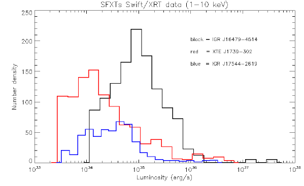
Figure 3: Distribution of the X–ray luminosity of three SFXTs we calculated from the X–ray count rate distribution observed with Swift, during a two years’ campaign. Data have been taken from Romano et al. (2010).

4.2 The model

In this section we interpret the observed luminosity distributions plotted in Fig. 3 in the light of the stochastic set up in the previous sections. Some of the questions we address are the following:

• The SFXTs’ luminosity distribution drops quite abruptly below $L_{X}\simeq 10^{33}-10^{34}{\leavevmode\nobreak\ \rm erg\,s^{-1}}$. Provided that this is not a selection effect in our observations, what is the origin of this feature?

• What properties of the accretion stream and accretion process can we infer by comparing our model with the observations? How do the properties of the stellar wind we deduce compare with the existing literature?

• Can we explain the difference between the wide dynamic range of luminosities observed in SFXTs and the much narrower one seen in persistent sources, like e.g. Vela X-1?

Our comparison of the model with the observed flares’ luminosity distributions (FLDs) is not intended to be a “best fitting” procedure, for several reasons.

First of all, our model (2) for the response of the accretor may be a bit oversimplified. The theoretical luminosity distribution $P$ computed from it, therefore, is not expected to provide an accurate model of the SFXT flares’ luminosity distribution observed in the real world . Second, only the FLDs of three sources are available for our analysis, probably too few to draw definite conclusions. Third, not all the flares may have been spotted during the observation campaign, and the FLDs we work with might not describe a fair sample of all the flares. Finally, the calculation of a model for given values of $\rho$ and $\sigma$ is quite time consuming, and a quantitative determination of those parameters via a best fitting procedure is not viable at the moment.

When we compare an observed FLD with its theoretical model, we aim to get a hint at the properties of the accretion process (described by the parameter $\rho$) and the properties of the family of clumps (described by the log-normal distribution (47)). A more physically motivated response is clearly necessary in order to make more quantitatively definite statements.

Despite its all too obvious limitations, we believe that our model has its own value. Its qualitative predictions are expected to hold even for a more sophisticated model; in addition it points out the fundamental properties of stochastic accretion that can be easily shaded by rather opaque mathematical complications that we leave to a forthcoming paper. That said, we are now ready to compare out theoretical predictions with the observed flares’ distributions in the three SFXTs IGR J$16479-4514$, IGR J$17544-2619$ and XTE J$1739-302$.

We aim at determining the best fitting parameters of our model from the flares’ distributions of a given SFXT. In general, the free parameters of the model are the accretion parameter $\rho$, the log-normal shape factor $\sigma$, the ratio $m_{0}/\tau$ and the cut-off mass accretion rate ${\dot{M}}_{\omega}$ due to the action of an accretion barrier (see Eq (29)). In order to keep things as simple as possible, in the following analysis we assume that no accretion barrier is present (i.e. ${\dot{M}}_{\omega}=0$), and the the model is completely defined by the three parameters $\rho$, $\sigma$ and $m_{0}/\tau$.

What is the best way to determine these parameters from the data of an observation campaign of a given SFXT? As we shall see, our choice is rather limited.

One might think, for instance, to determine the parameters by comparing the mean, variance, skewness and excess kurtosis computed from our model (see Eq. (43)) with the observed mean, variance, skewness and excess kurtosis, provided that we are able to convert the mass accretion rate ${\dot{M}}$ to a X–ray luminosity. If there is no accretion barrier, the modelled luminosity distribution is simply $p(L)=P(x)/L_{\ast}$, where $P(x)$ is the dimensionless distribution computed from the generalized Fokker–Planck equation, and

$$L_{\ast}=\frac{G\,{M_{\rm ns}}\,m_{0}}{{R_{\rm ns}}\,\tau},$$ (50)

where ${M_{\rm ns}}\sim 1.4{\leavevmode\nobreak\ M_{\odot}}$ and ${R_{\rm ns}}\sim 10\leavevmode\nobreak\ \rm km$ are the typical mass and radius of a neutron star. A direct comparison of the moments of the theoretical and the computed distributions, however, is not viable. The use of high order momenta such as the skewness or the kurtosis of a heavy tailed distribution (like our $P(x)$) is not recommended for any statistical analysis (e.g. Press et al., 2007). The problem is that these moments are not robust, i.e. they are too sensitive to the outliers. Any small change in the number of the observed high luminosity flares would alter the values of these moments considerably, making them of little use to any statistical purpose.

Since we cannot use the moments, we are forced to determine the parameters by comparing the full shapes of the observed and the theoretical distributions. The data from Romano et al. (2010) available to our analysis are already binned in luminosity intervals: we known the fraction $P_{i}^{(\rm obs)}$ of the flares observed in the luminosity interval $[L_{i},L_{i+1}$], but we don’t have access to the luminosity of each single flare. This prevents us from using any variant of the Kolmogorov–Smirnov test to compare the theoretical and the observed flares’ distributions.

For these reasons, we must resort to a least squares method to determine the parameters $\rho$, $\sigma$ and $m_{0}/\tau$. Suppose for the moment that $\rho$ and $\sigma$ are known, and the only parameter to be determined is $m_{0}/\tau$. For a (tentative) value of $m_{0}/\tau$ we compute the scale luminosity (50) and the expected fraction $P_{i}^{({\rm cal})}$ of flares within the luminosity interval $[L_{i},L_{i+1}$]. We compute the chi-squared

$$\mathcal{X}^{2}=\sum_{i}\frac{\left[P_{i}^{(\rm obs)}-P_{i}^{(\rm cal)}\right]^{2}}{\sigma_{i}^{2}},$$ (51)

where we assume the errors on the observed fractions $\sigma_{i}^{2}\sim P_{i}^{(\rm cal)}$. Finally, we find the value of $m_{0}/\tau$ that minimises $\mathcal{X}^{2}$. A minimisation procedure to determine all the parameters $\rho$, $\sigma$ and $m_{0}/\tau$ would be very time consuming, and therefore is not viable at the moment. For this reason we have built a grid of values of $\rho$ and $\sigma$, and for each couple ($\rho$, $\sigma$) we have computed the correspondent $P(x)$, and the value of $m_{0}/\tau$ that minimises the $\mathcal{X}^{2}$ for that $P$. Finally, we chose as our best estimates for $\rho$, $\sigma$ and $m_{0}/\tau$ the values that return the smallest $\mathcal{X}^{2}$. On account of the (expected) poor quality of the fits, we do not report the values of the $\mathcal{X}^{2}$ statistics, but we only discuss here below our results.

Fig. 4 shows the flares’ distributions for our three SFXTs superposed to their “best fitting” models. On account of the asymptotic behaviour (44) of the theoretical luminosity distribution, a glance to Fig. 3 hints that in all cases it must be $\rho>1$ to match the observed FLDs. In addition, the observed high dynamical ranges of the flares’ luminosities require a heavy tailed clumps’ mass distribution, i.e. a relatively high log-normal shape parameter $\sigma$.

Figure 4: The observed FLDs of the SFXTs $IGR\leavevmode\nobreak\ J17544-2619$ (top panel), $IGR\leavevmode\nobreak\ J16479-4514$ (middle panel) and $XTE\leavevmode\nobreak\ J1739-302$ (bottom panel) superposed to their “best fitting” theoretical curves. The closest agreement between the observed and the computed FLD are found for $\rho=8$, $\sigma=4$ and $m_{0}/\tau=1.0\times 10^{12}{\leavevmode\nobreak\ \rm g}{\leavevmode\nobreak\ \rm s}^{-1}$. (for $IGR\leavevmode\nobreak\ J17544-2619$), $\rho=10$, $\sigma=5$ and $m_{0}/\tau=5.5\times 10^{11}{\leavevmode\nobreak\ \rm g}{\leavevmode\nobreak\ \rm s}^{-1}$ (for $IGR\leavevmode\nobreak\ J16479-4514$) and $\rho=40$, $\sigma=8$ and $m_{0}/\tau=1.0\times 10^{7}{\leavevmode\nobreak\ \rm g}{\leavevmode\nobreak\ \rm s}^{-1}$ (for $XTE\leavevmode\nobreak\ J1739-302$).

$IGR\leavevmode\nobreak\ J17544-2619$ is the source with the lowest dynamic range, since it displayed flares ranging in the luminosity interval between $3.9\times 10^{33}{\leavevmode\nobreak\ \rm erg\,s^{-1}}$ and $2.7\times 10^{36}{\leavevmode\nobreak\ \rm erg\,s^{-1}}$. There is no apparent low luminosity cut–off (which might be interpreted as the effect of an accretion barrier). The FLD of this source may be reproduced quite nicely by a model with $\rho=8$, $\sigma=4$ and $m_{0}/\tau=1.0\times 10^{12}{\leavevmode\nobreak\ \rm g}{\leavevmode\nobreak\ \rm s}^{-1}$.

The source $IGR\leavevmode\nobreak\ J16479-4514$ has the highest dynamic range of all the considered sources, with flares’ luminosities ranging from $1.4\times 10^{34}{\leavevmode\nobreak\ \rm erg\,s^{-1}}$ to $3.5\times 10^{37}{\leavevmode\nobreak\ \rm erg\,s^{-1}}$. In this case the best value of the log-normal shape is $\sigma=5$ (slightly larger than the value found for $IGR\leavevmode\nobreak\ J17544-2619$). The best estimate of the accretion parameter is $\rho=10$, and even in this case it is not probably necessary to invoke an accretion barrier to explain the left tail of the observed FLD. The last parameter is $m_{0}/\tau=5.5\times 10^{11}{\leavevmode\nobreak\ \rm g}{\leavevmode\nobreak\ \rm s}^{-1}$.

The flares of $XTE\leavevmode\nobreak\ J1739-302$ show luminosities between $3.3\times 10^{33}{\leavevmode\nobreak\ \rm erg\,s^{-1}}$ and $5.3\times 10^{36}{\leavevmode\nobreak\ \rm erg\,s^{-1}}$. Its steep “wall” that cuts off $S(L)$ below $L=2.1\times 10^{33}{\leavevmode\nobreak\ \rm erg\,s^{-1}}$ is difficult to reproduce. Following our discussion of the “$\rho$ suppression” at the end of Sec. 3.1, one might expect that a very high value of $\rho$ is necessary to cut off abruptly the low tail of the luminosity distribution. Indeed, our best-fitting model for this source gives $\rho=40$, $\sigma=8$ and $m_{0}/\tau=1.0\times 10^{7}{\leavevmode\nobreak\ \rm g}{\leavevmode\nobreak\ \rm s}^{-1}$. We note however that the space of parameters characterised by high values of $\rho$ and $\sigma$ is quite difficult to explore with our means. For this reason, and also on account of the relatively poor quality of the “best fit” shown at the bottom panel of Fig. 4, we cannot be sure that the $\rho$ suppression is winning over the “propeller barrier” process discussed in Sec. 2.1.

To resume, we may reproduce at least the gross properties of the sources’ FLDs, with moderate values of the accretion parameter $\rho$ and a relatively high shape parameters $\sigma$ of the clumps’ log-normal. At least two of our sources do not require any accretion barrier to explain their low luminosity tail, that may be justified by the “$\rho$ suppression”. The source $XTE\leavevmode\nobreak\ J1739-302$ is more problematic, and here a propeller barrier is not excluded.

Our model has three degrees of freedom: $m_{0}/\tau$, $\sigma$ and the accretion parameter $\rho\equiv\lambda\,\tau$. The mass arrival rate $\lambda$ is degenerate since it only appears in a product with $\tau$ in the accretion parameter $\rho$, and so it cannot be determined directly from a comparison of our model with the observations. We may however get a hint from the analysis of the flares’ light curves and from the geometry of the system.

In their analysis of the light curve of $IGR\leavevmode\nobreak\ J16479-4514$ Sguera et al. (2005) found that the flares lasted from $\sim 30\leavevmode\nobreak\ \rm min$ to $\sim 3\leavevmode\nobreak\ \rm h$. In one case, they were able to analyse a single light curve that after a fast rise, decayed exponentially with an e-folding time $\tau=15\pm 9\leavevmode\nobreak\ \rm min$. Exponentially decaying light curves are not uncommon for the flares occurring in this source (Ducci et al., 2010). If the decay time $\tau\sim 10^{3}{\leavevmode\nobreak\ \rm s}$ may be taken as typical, then for $\rho\sim 10$ we estimate the time interval between the successive accretion of two clumps $\lambda^{-1}\sim 10^{2}{\leavevmode\nobreak\ \rm s}$. If the NS orbits a massive star of $M\simeq 20{\leavevmode\nobreak\ M_{\odot}}$ with a period $P_{\rm orb}\simeq 3\leavevmode\nobreak\ \rm d$ (typical of $IGR\leavevmode\nobreak\ J16479-4514$), the distance covered by the NS between two successive encounters is of the order of few $10^{9}{\leavevmode\nobreak\ \rm cm}$, a fraction of the stellar radius. From the values of $m_{0}/\tau$ and $\tau\sim 10^{3}{\leavevmode\nobreak\ \rm s}$ we find values of $m_{0}$ between $\sim 10^{10}{\leavevmode\nobreak\ \rm g}$ and $\sim 10^{15}{\leavevmode\nobreak\ \rm g}$ for our three sources. On account of the large values of $\sigma$, the mean masses are much larger than these (compare with Eq. (48)), and are of the order of $10^{18}-10^{21}{\leavevmode\nobreak\ \rm g}$. These values for the clumpy wind are in broad agreement with estimates obtained with other means (see e.g. Ducci et al., 2009).

We now present a simple argument showing how the parameters $m_{0}/\tau$, $\sigma$ and $\rho$ may not be fully independent of each other. Consider a giant donor star with mass $M_{\star}$ and radius $R_{\star}$ that blows a clumpy wind. Assuming that the mass carried by the wind is all in clumps, then the mean stellar mass outflow rate at the distance $r$ from the star is

$${\dot{M}}_{w}=4\,\pi\,r^{2}\,n_{\rm cl}\,v_{\rm cl}\,{\langle{m}\rangle},$$ (52)

where $n_{\rm cl}$ is the mean number of clumps per unit volume, and $v_{\rm cl}$ is the mean clumps’ velocity. As the neutron star orbits the giant star, it crosses this clumpy wind and encounter clumps with the mean rate

$$\lambda=\pi\,R_{G}^{2}\,v_{\rm orb}\,n_{\rm cl},$$ (53)

where $v_{\rm orb}$ is the orbital velocity of the NS and $R_{G}$ is the capture radius defined by Eq. (24). Eliminating $n_{\rm cl}$ from Eqns. (52) and (53) and postulating that the population of the masses is log-normally distributed with shape parameter $\sigma$ and median mass $m_{0}$ we find

$$\lambda=\left(\frac{R_{G}}{2\,r}\right)^{2}\;\frac{{\dot{M}}_{w}}{m_{0}}\;\frac{v_{\rm orb}}{v_{\rm cl}}\;{\rm e}^{-\sigma^{2}/2}$$ (54)

The rate $\lambda$ is a strongly decreasing function of the clumps’ mass distribution shape $\sigma$ for the following simple reason. If $\sigma$ is large, the log-normal distribution is skewed to the right, and most of the mass blown by the wind is carried by large, heavy clumps. A given ${\dot{M}}_{w}$ is carried by relatively few clumps, and their encounters with the orbiting neutron star are rare, i.e. $\lambda$ is small. Multiplying the last equation by $\tau$, we find

$$\rho=\left(\frac{R_{G}}{2\,r}\right)^{2}\;\frac{{\dot{M}}_{w}}{m_{0}/\tau}\;\frac{v_{\rm orb}}{v_{\rm cl}}\;{\rm e}^{-\sigma^{2}/2}.$$ (55)

This shows that in our model the parameters $\sigma$, $\rho$ and $m_{0}/\tau$ are not independent of each other: $\rho$ is proportional to $(m_{0}/\tau)^{-1}$ and decreases exponentially with $\sigma^{2}/2$. It is difficult to use this equation to make quantitative predictions about the magnitude of $\rho$ as a function of the other parameters. Indeed, when made explicit, its right hand side is found to be very sensitive to the values of rather uncertain quantities (e.g. the velocity of the stellar wind), and even a small change in their value may vary $\rho$ by orders of magnitude. We may plug the values of $\lambda$ and $\rho$ into Eqns. (49) to find

$$\frac{\sigma_{L}}{{\langle{L}\rangle}}=\left(2\>\frac{m_{0}/\tau}{{\dot{M}}_{w}}\;\frac{v_{\rm cl}}{v_{\rm orb}}\right)^{1/2}\;\frac{r}{R_{G}}\;{\rm e}^{3\sigma^{2}/4},$$ (56)

where ${\langle{L}\rangle}$ and $\sigma_{L}$ are respectively the mean accretion luminosity and the standard deviation of $L$, if $L\propto{\dot{M}}$. The exponential factor at the right hand side of the Eq. (56) suggests an explanation for the difference between the ordinary, persistent X–ray sources occurring in the high mass binaries, and the SFXTs. Indeed, according to Eq. (56), even moderate values of $\sigma$ (say, $\sigma\simeq 4-5$) greatly amplify the dispersion around the mean $\sigma_{L}/{\langle{L}\rangle}$. This means that the wide dynamical range of luminosities observed in SFXTs is but the effect of the accretion of a population of clumps with a wide mass spectrum $\varphi(m)$. On the other hand, if $\sigma\ll 1$, i.e. all the accreting clumps have very similar masses, there is no such strong amplification, and $\sigma_{L}/{\langle{L}\rangle}$ may be small. The FLD generated by the accretion of clumps with narrowly distributed masses should resemble the distribution $P$ discussed in Sec. 3.2.

According to this model, then, the difference between persistent HMXBs and SFXTs is entirely due to a substantial difference between the winds blown by the donor stars hosted in these systems. Since SFXTs are much rarer than the ordinary HMXBs, probably the occurrence of a clumpy stellar wind with a wide range of masses is also a rare event.

5 Summary and conclusions

In this paper we have set up a simple stochastic model for the accretion of a clumpy stream on a compact object. We have modelled the response of the compact object to the accretion with a simple exponential law (2) characterised by the relaxation time $\tau$. The accretion stream is described as a train of pulses hitting the compact object with the mean rate $\lambda$. The clumps have a mass distribution described by the function $\varphi(m)$. With these ingredients we have written a stochastic differential equation (SDE) for the mass accretion rate ${\dot{M}}(t)$. We have also derived the generalised Fokker–Planck equation (GFPE) associated to the SDE. Its solution $P({\dot{M}},t)$ is the probability that the mass accretion rate is ${\dot{M}}$ at the time $t$. We have then restricted us to the analysis of the stationary solution $P({\dot{M}})$. In general $P$ cannot be written in a closed form for any choice of $\varphi$, but it is nevertheless possible to express its moments as functions of the moments of $\varphi$ (if they exist). In addition, the asymptotic behaviour of $P({\dot{M}})$ for small ${\dot{M}}$ is $P({\dot{M}})\propto{\dot{M}}^{\rho-1}$, for any $\varphi(m)$ limited for small $m$. For $\rho\gg 1$, then, $P({\dot{M}})$ is negligible for ${\dot{M}}\lesssim m_{0}/\tau$. This “$\rho$ suppression” of $P$ occurs when the relaxation time $\tau$ is long with respect to the clumps’ arrival rate, and the compact object cannot respond promptly enough to the rapid succession of clumps’ arrivals (Sec. 3.1).

We have then studied in some detail the function $P$ for two choices of $\varphi$: a delta function and a log-normal distribution. In the case of a log-normal $\varphi$, $P$ depends on three parameters: the accretion parameter $\rho\equiv\lambda\,\tau$, $m_{0}/\tau$ and $\sigma$, where $m_{0}$ and $\sigma$ are the location and shape parameters of the log-normal.

As a case study, we have applied our formalism (with a log-normal $\varphi$) to the physics of Super Giant Fast X–ray Transients (SFXTs), a peculiar sub-class of High Mass X–ray binaries (HMXBs).

We have compared our model to the flares’ X-ray luminosity distributions of the SFXTs $IGR\leavevmode\nobreak\ J17544-2619$, $IGR\leavevmode\nobreak\ J16479-4514$ and $XTE\leavevmode\nobreak\ J1739-302$ observed in a two years’ campaign with Swift.

We have found that, however simplified, our model may reproduce the features of the observed flares’ distributions. The typical parameters giving the best agreement between the model and the observations are $\rho\sim 10$ and $\sigma\sim 5$, corresponding to a long tail in the mass distributions. The parameters $\tau$ and $\lambda$ cannot be determined separately, but taking the value $\tau\simeq 10^{3}{\leavevmode\nobreak\ \rm s}$ suggested by some observations, we find $\lambda^{-1}\sim 10^{2}{\leavevmode\nobreak\ \rm s}$, or an inter-clump average distance $10^{9}-10^{10}{\leavevmode\nobreak\ \rm cm}$. The average masses of the clumps are in the order of $10^{18}-10^{21}{\leavevmode\nobreak\ \rm g}$, in broad agreement with the estimates found in the existing literature (e.g. Ducci et al., 2009). In at least two of the SFXTs we analysed, we were able to reproduce the flares’ luminosity distributions without invoking an accretion barrier.

The reason why SFXT show a much higher dynamic range than the ordinary HMXBs is still unclear: according to our model, the difference is entirely due to the different properties of the streams of matter accreting the compact objects hosted in those systems. HMXBs accrete from clumpy winds with a narrow mass distribution, while SFXTs from winds with an extremely wide clumps’ mass distribution. In a recent paper Oskinova et al. (2012) pointed out that a stochastic component in the clumps’ velocities is probably essential in shaping the light curves of SFXTs. In the present paper we have neglected the possible contributions to $L(t)$ from a stochastic component of the velocity of the accreting stream, but it must clearly be included in any (more) realistic model.

Appendix A Derivation of the generalized Fokker–Planck Equation

In this section we closely follow Denisov et al. (2009) to derive the generalized Fokker–Planck equation (30a) from the Langevin Equation (7). According to the Ito interpretation, the solution of Eq. (7) in the (short) time interval $\Delta t$ is

$${\dot{M}}(t+\Delta\,t)={\dot{M}}(t)-\Delta\,t\,{\dot{M}}(t)/\tau+\delta M_{c}(t)/\tau,$$ (A1)

where

$$\delta M_{c}(t)=\int_{t}^{t+\Delta\,t}dt^{\prime}\>{\dot{M}}_{c}(t^{\prime})=\sum_{k=1}^{n(\Delta t)}m_{k},$$ (A2)

being $n(\Delta t)$ is the number of clumps accreted in the time interval $\Delta t$.

In order to derive the generalised Fokker–Planck equation we introduce the probability $p(\Delta M,\Delta t)$ that the mass $\Delta M$ is accreted by the compact object in the interval $\Delta t$

$$p(\Delta M,\Delta t)={\langle{\delta(\Delta M-\delta M_{c}(t))}\rangle}.$$ (A3)

From this definition and Eq. (A3), after some algebra it can be shown that

$$p(\Delta M,\Delta t)=P_{0}(\Delta t)\;\delta(\Delta M)+W(\Delta M,\Delta t)$$ (A4a)

where

$$W(\Delta M,\Delta t)=\sum_{k=1}^{\infty}P_{k}(\Delta t)\;\int dm_{1}\;\varphi(m_{1})\int dm_{2}\;\varphi(m_{2})\cdots\int dm_{k}\;\varphi(m_{k})\;\delta\left(\Delta M-\sum_{j=1}^{k}m_{j}\right),$$ (A4b)

being $P_{n}(\Delta t)$ the Poisson probability that $n$ clumps are accreted in the time interval $\Delta t$, and $\varphi(m)$ is the mass distribution of the clumps. If $\Delta t$ is small, we may expand $p$ to first order in $\Delta t$ and take

$$p(\Delta M,\Delta t)=(1-\lambda\Delta t)\;\delta(\Delta M)+\lambda\Delta t\;\varphi(\Delta M)+{\mathcal{O}}(\Delta t)$$ (A5)

The accretion probability $P({\dot{M}},t)$ is defined as

$$P({\dot{M}},t)=\langle\delta({\dot{M}}-{\dot{M}}(t)\rangle.$$ (A6)

In order to proceed, we need a couple of formulae to express the averages of the functions ${\langle{F({\dot{M}}(t))}\rangle}$ and ${\langle{F({\dot{M}}(t),\delta M_{c}(t))}\rangle}$ in terms of the accretion probability distributions $P({\dot{M}},t)$ and $p(\Delta M,\Delta t)$. Since the random variable ${\dot{M}}(t)$ and $\delta M_{c}(t)$ are independent, then

$${\langle{F({\dot{M}}(t))}\rangle}=\int d{\dot{M}}\;P({\dot{M}},t)\;F({\dot{M}})$$ (A7a)

and

$${\langle{F({\dot{M}}(t),\delta M_{c}(t))}\rangle}=\int d{\dot{M}}\;\int d(\Delta M)\;P({\dot{M}},t)\;p(\Delta M,\Delta t)\;F({\dot{M}},\Delta M).$$ (A7b)

We now introduce the time Fourier transformation to derive the generalised Fokker–Planck equation. From the definition it is clear that

$$P_{k}(t)=\int d{\dot{M}}\;P({\dot{M}},t)\;{\rm e}^{-ik{\dot{M}}}={\langle{{\rm e}^{-ik{\dot{M}}}}\rangle}.$$ (A8)

We calculate the increment $\delta P_{k}(t)=P_{k}(t+\Delta t)-P_{k}(t)$ from Eq. (A1) as

$$\delta P_{k}(t)=\left\langle{\rm e}^{-ik{\dot{M}}(t+\Delta t)}-{\rm e}^{-ik{\dot{M}}(t)}\right\rangle$$ (A9)

Expressing ${\dot{M}}(t+\Delta t)$ with Eq. (A1) and retaining only the terms linear in $\Delta t$,

$$\delta P_{k}(t)=\left\langle{\rm e}^{-ik{\dot{M}}(t)}\left[{\rm e}^{-ik\delta{\dot{M}}_{c}(t)/\tau}-1\right]\right\rangle+ik\frac{\Delta t}{\tau}\left\langle{\dot{M}}(t)\>{\rm e}^{-ik{\dot{M}}(t)}\right\rangle+{\mathcal{O}}(\Delta t)$$ (A10)

Introducing the probability distributions $P$ and $p$,

$$\delta P_{k}(t) = \int d{\dot{M}}\;P({\dot{M}},t){\rm e}^{-ik{\dot{M}}}\int d(\Delta M)p(\Delta M,\Delta t)\left[{\rm e}^{-ik\delta{\dot{M}}_{c}(t)/\tau}-1\right]+$$ (A12)

$$+ik\frac{\Delta t}{\tau}\int d{\dot{M}}P({\dot{M}},t){\dot{M}}\>{\rm e}^{-ik{\dot{M}}}+{\mathcal{O}}(\Delta t).$$

Plugging Eq. (A5) into this expression we obtain

$$\delta P_{k}(t) = \int d{\dot{M}}\;P({\dot{M}},t){\rm e}^{-ik{\dot{M}}}\lambda\,\Delta t\>\int d(\Delta M)\varphi(\Delta M)\left[{\rm e}^{-ik\delta{\dot{M}}_{c}(t)/\tau}-1\right]+$$ (A14)

$$+ik\frac{\Delta t}{\tau}\int d{\dot{M}}P({\dot{M}},t){\dot{M}}\>{\rm e}^{-ik{\dot{M}}}+{\mathcal{O}}(\Delta t)$$

Dividing by $\Delta t$ and sending $\Delta t\to 0$

$$\frac{\partial P_{k}}{\partial t}=\lambda P_{k}\;\varphi_{k/\tau}-\lambda\>P_{k}+i\frac{k}{\tau}\int d{\dot{M}}P({\dot{M}},t){\dot{M}}\>{\rm e}^{-ik{\dot{M}}}.$$ (A15)

Finally, the inverse Fourier transform yields

$$\frac{\partial P}{\partial t}=-\lambda P\;+\lambda\int_{0}^{{\dot{M}}\,\tau}dm\>\varphi(m)\;P\left({\dot{M}}-m/\tau,t\right)+\frac{1}{\tau}\;\frac{\partial}{\partial{\dot{M}}}\left({\dot{M}}\,P\right),$$ (A16)

which is the desired Fokker–Planck equation.

References

- Abramowitz and Stegun (1972) Abramowitz, M. and Stegun, I. A.: 1972, Handbook of Mathematical Functions, Dover, New York
- Barenblatt (1996) Barenblatt, G. I.: 1996, Scaling, Self-similarity, and Intermediate Asymptotics, Cambridge University Press, Cambridge, UK
- Bozzo et al. (2008) Bozzo, E., Falanga, M., and Stella, L.: 2008, ApJ 683, 1031
- Davies et al. (1979) Davies, R. E., Fabian, A. C., and Pringle, J. E.: 1979, MNRAS 186, 779
- Davies and Pringle (1981) Davies, R. E. and Pringle, J. E.: 1981, MNRAS 196, 209
- Denisov et al. (2009) Denisov, S. I., Horsthemke, W., and Hänggi, P.: 2009, European Physical Journal B 68, 567
- Drave et al. (2010) Drave, S. P., Clark, D. J., Bird, A. J., McBride, V. A., Hill, A. B., Sguera, V., Scaringi, S., and Bazzano, A.: 2010, MNRAS 409, 1220
- Ducci et al. (2009) Ducci, L., Sidoli, L., Mereghetti, S., Paizis, A., and Romano, P.: 2009, MNRAS 398, 2152
- Ducci et al. (2010) Ducci, L., Sidoli, L., and Paizis, A.: 2010, MNRAS 408, 1540
- Frank et al. (2002) Frank, J., King, A., and Raine, D. J.: 2002, Accretion Power in Astrophysics, Cambridge University Press, Cambridge, UK, third edition
- Gardiner (2009) Gardiner, C. W.: 2009, Stochastic Methods, A Handbook for the Natural and Social Sciences, Springer Verlag, Berlin Heidelberg New York
- Grebenev and Sunyaev (2007) Grebenev, S. A. and Sunyaev, R. A.: 2007, Astronomy Letters 33, 149
- Illarionov and Sunyaev (1975) Illarionov, A. F. and Sunyaev, R. A.: 1975, A&A 39, 185
- in’t Zand (2005) in’t Zand, J. J. M.: 2005, A&A 441, L1
- Kloeden and Platen (1999) Kloeden, P. E. and Platen, E.: 1999, Numerical Solution of Stochastic Differential Equations, Springer Verlag, Berlin, Heidelberg, New York
- Lipunov (1987) Lipunov, V. M.: 1987, Ap&SS 132, 1
- Mori and Sugihara (2001) Mori, M. and Sugihara, M.: 2001, J. Comput. Appl. Math. 127, 287
- Negueruela et al. (2006) Negueruela, I., Smith, D. M., Reig, P., Chaty, S., and Torrejón, J. M.: 2006, in A. Wilson (ed.), Proc. of the “The X-ray Universe 2005”, 26-30 September 2005, El Escorial, Madrid, Spain. ESA SP-604, Volume 1, Noordwijk: ESA Pub. Division, ISBN 92-9092-915-4, 2006, p. 165
- Negueruela et al. (2008) Negueruela, I., Torrejón, J. M., Reig, P., Ribó, M., and Smith, D. M.: 2008, in R. M. Bandyopadhyay, S. Wachter, D. Gelino, and C. R. Gelino (eds.), A Population Explosion: The Nature & Evolution of X-ray Binaries in Diverse Environments, Vol. 1010 of American Institute of Physics Conference Series, pp 252–256
- Øksendal (2003) Øksendal, B.: 2003, Stochastic Differential Equations, Springer Verlag, Berlin, Heidelberg, New York, sixth edition
- Ooura and Mori (1999) Ooura, T. and Mori, M.: 1999, J. Comput. Appl. Math. 112, 229, 241
- Oskinova et al. (2012) Oskinova, L. M., Feldmeier, A., and Kretschmar, P.: 2012, ArXiv e-prints
- Pizzolato and Soker (2005) Pizzolato, F. and Soker, N.: 2005, ApJ 632, 821
- Press et al. (2007) Press, W. H., Teukolsky, S. A., Vetterling, W. T., and Flannery, B. P.: 2007, Numerical Recipes in C++. The Art of Scientific Computing, Cambridge University Press, Cambridge, UK, third edition
- Puls et al. (2008) Puls, J., Vink, J. S., and Najarro, F.: 2008, A&A Rev. 16, 209
- Rampy et al. (2009) Rampy, R. A., Smith, D. M., and Negueruela, I.: 2009, ApJ 707, 243
- Reif (1965) Reif, F.: 1965, Fundamentals of Statistical and Thermal Physics, Dover, New York
- Romano et al. (2010) Romano, P., La Parola, V., Vercellone, S., Cusumano, G., Sidoli, L., Krimm, H. A., Pagani, C., Esposito, P., Hoversten, E. A., Kennea, J. A., Page, K. L., Burrows, D. N., and Gehrels, N.: 2010, MNRAS pp 1535–1547
- Romano et al. (2007) Romano, P., Sidoli, L., Mangano, V., Mereghetti, S., and Cusumano, G.: 2007, A&A 469, L5
- Sguera et al. (2005) Sguera, V., Barlow, E. J., Bird, A. J., Clark, D. J., Dean, A. J., Hill, A. B., Moran, L., Shaw, S. E., Willis, D. R., Bazzano, A., Ubertini, P., and Malizia, A.: 2005, A&A 444, 221
- Sguera et al. (2006) Sguera, V., Bazzano, A., Bird, A. J., Dean, A. J., Ubertini, P., Barlow, E. J., Bassani, L., Clark, D. J., Hill, A. B., Malizia, A., Molina, M., and Stephen, J. B.: 2006, ApJ 646, 452
- Shakura and Sunyaev (1973) Shakura, N. I. and Sunyaev, R. A.: 1973, A&A 24, 337
- Sidoli (2011) Sidoli, L.: 2011, Proc. of the conference “The Extreme and Variable High Energy Sky”, September 19-23, 2011, Chia Laguna, Sardegna (Italy); PoS(Extremesky 2011)010; eprint arXiv:1111.5747
- Sidoli et al. (2008) Sidoli, L., Romano, P., Mangano, V., Pellizzoni, A., Kennea, J. A., Cusumano, G., Vercellone, S., Paizis, A., Burrows, D. N., and Gehrels, N.: 2008, ApJ 687, 1230
- Sidoli et al. (2007) Sidoli, L., Romano, P., Mereghetti, S., Paizis, A., Vercellone, S., Mangano, V., and Götz, D.: 2007, A&A 476, 1307
- Warner (1995) Warner, B.: 1995, Cataclysmic Variable Stars, Cambridge University Press, Cambridge, UK