Determination of the strong coupling $\alpha_{s}$ from the QCD static energy

Abstract:

We obtain a determination of the strong coupling $\alpha_{s}$ in quantum chromodynamics, by comparing perturbative calculations for the short-distance part of the static energy with lattice computations. Our result reads $\alpha_{s}\left(1.5{\rm GeV}\right)=0.326\pm 0.019$, and when evolved to the scale $M_{Z}$ (the $Z$-boson mass) it corresponds to $\alpha_{s}\left(M_{Z}\right)=0.1156^{+0.0021}_{-0.0022}$.

This talk is based on Ref. [1]. The reader is referred to that paper for additional explanations.

1 Introduction

The energy between a static (i.e. infinitely heavy) quark and a static antiquark separated a distance $r$ is known as the quantum chromodynamics (QCD) static energy, $E_{0}(r)$, and is a basic object to understand the dynamics of the theory. As it is well known, one can distinguish a long-distance part and a short-distance part of the static energy. The long-distance part encodes the confining dynamics of the theory, whereas the short-distance part can be computed in perturbation theory. On the other hand, one can use lattice QCD simulations to compute the static energy in both (short- and long- distance) regimes. Here we want to focus only on the short-distance part of the static energy, where the perturbative weak-coupling approach is expected to be reliable. In particular, we want to compare state-of-the-art perturbative calculations with the lattice results. This comparison allows us to obtain a determination of the strong coupling $\alpha_{s}$, which is the main outcome of the present analysis.

2 Perturbative calculation

At short distances, $E_{0}(r)$ is given at leading order by the Coulomb potential (with the adequate color factor), $E_{0}(r)\sim-C_{F}\alpha_{s}/r$ (where $C_{F}=(N_{c}^{2}-1)/(2N_{c})$, and $N_{c}$ is the number of colors), and then we have corrections to this result. At present the static energy is known including terms up to order $\alpha_{s}^{4+n}\ln^{n}\alpha_{s}$ with $n\geq 0$ [2, 3, 4, 5, 6, 7, 8] (a level of accuracy which we refer to as next-to-next-to-next-to leading logarithmic -N³LL-). The presence of $\ln\alpha_{s}$ terms in the expansion of the static energy is due to the virtual emissions of gluons with energy of order $E_{0}$ (the so-called ultrasoft gluons), that can change the color state of the quark-antiquark pair from singlet to octet and vice versa [9, 10]. Detailed expressions for the static energy at this level of accuracy were given in Ref. [2] (and references therein; see also [11] for explicit numerical expressions), and we will not reproduce them here.

3 Lattice computation

The static energy has been recently calculated in $2+1$ flavor lattice QCD [12]. This computation used a combination of tree-level improved gauge action and highly-improved staggered quark action [13]; it employed the physical value for the strange-quark mass $m_{s}$ and light-quark masses equal to $m_{s}/20$ (corresponding to pion masses of about 160MeV). It was performed for a wide range of gauge couplings, $5.9\leq\beta\equiv 10/g^{2}\leq 7.28$. At each value of the gauge coupling one calculates the scale parameters $r_{0}$ and $r_{1}$, defined in terms of the static energy $E_{0}(r)$ as follows [14, 15]

$$r^{2}\frac{dE_{0}(r)}{dr}|_{r=r_{0}}=1.65,~{}~{}~{}r^{2}\frac{dE_{0}(r)}{dr}|_{r=r_{1}}=1.$$ (1)

The values of $r_{0}$ and $r_{1}$ were given in Ref. [12] for each $\beta$. The above range of gauge couplings corresponds to lattice spacings $1.909/r_{0}\leq a^{-1}\leq 6.991/r_{0}$. Using the most recent value $r_{0}=0.468\pm 0.004$ fm [12] we get $0.805\,{\rm GeV}<a^{-1}<2.947\,{\rm GeV}$. Thus we can study the static energy down to distances $r=0.14r_{0}$ or $r\simeq 0.065$ fm. For the comparison with perturbation theory the most relevant data set is the one that corresponds to $\beta=6.664,6.740,6.800,6.880,6.950,7.030,7.150,7.280$, which is what we use here. The static energy can be calculated in units of $r_{0}$ or $r_{1}$. Since the static energy has an additive ultraviolet renormalization (self energy of the static sources) one needs to normalize the results calculated at different lattice spacings to a common value at a certain distance (or alternatively one can take a derivative and compute the force). The static energy is fixed, in units of $r_{0}$, to 0.954 at $r=r_{0}$ [12]. At distances comparable to the lattice spacing the static energy suffers from lattice artifacts. To correct for these artifacts we use tree level improvement. That is, from the lattice Coulomb potential

$$C_{L}(r)=\int\frac{d^{3}k}{(2\pi)^{3}}D_{00}(k_{0}=0,\vec{k})e^{i\vec{k}\vec{r}},$$ (2)

we can define the improved distance $r_{I}=(4\pi C_{L}(r))^{-1}$ for each separation $r$. Here $D_{00}$ is the tree level gluon propagator for the $a^{2}$ improved gauge action. The tree level improvement amounts to replacing $r$ by $r_{I}$ [16]. Alternatively following Ref. [15, 17] we fit the lattice data at short distances to the form $const-a/r+\sigma r+a^{\prime}(1/r-1/r_{I})$ and subtract the last term from the lattice data. Since the data at the shortest distances that we use (for each $\beta$) correspond to a separation of one lattice spacing, it is important to check that the way we are using to correct lattice artifacts is working properly. In that sense, we have found that both methods of correcting for lattice artifacts lead to the same results within errors of the calculations. Furthermore, the static energies calculated for different lattice spacings agree well with each other after the removal of lattice artifacts, and when one puts all the data together it seems to lie on a single curve, even at short distances, indicating that the above procedure of removing the lattice artifacts works.

4 Comparing lattice and perturbation theory: $\alpha_{s}$ extraction

We can now compare the lattice results with the perturbative expressions, and use the comparison to extract the value of the QCD scale $\Lambda_{\overline{\rm MS}}$ (in the $\overline{\rm MS}$ scheme). In order to obtain this extraction, we assume that perturbation theory (after implementing a cancellation of the leading renormalon singularity) is enough to describe lattice data in the range of distances we are considering (we use lattice data for $r<0.5r_{0}$, and since we have lattice data points down to $r=0.14r_{0}$, this means that we are studying the static energy in the 0.065 fm$\lesssim r\lesssim$0.234 fm distance range, in physical units). Then we search for the values of $\Lambda_{\overline{\rm MS}}$ that are allowed by lattice data; the guiding principle to do that is that the agreement with lattice should improve when the perturbative order of the calculation is increased.

As it was already mentioned above, in the perturbative calculation of the energy one needs to implement a scheme that cancels the leading renormalon singularity [18, 19]. This kind of schemes introduce an additional dimensional scale in the problem (that we denote as $\rho$). We implement the renormalon cancellation according to the RS-scheme described in Ref. [20]. The static energy in this scheme is given by

$$E_{0}^{\rm RS}(r,\rho)=E_{0}^{\overline{\rm MS}}(r)-\textrm{RS\small{subtr.}}(\rho),$$ (3)

where the subtraction term on the right-hand side cancels the leading renormalon singularity of $E_{0}^{\overline{\rm MS}}(r)$; the explicit expression for $\textrm{RS\small{subtr.}}(\rho)$ is given, for instance, in Eq. (7) of Ref. [11]. The scale $\rho$ has, in this case, a natural value which corresponds to the center of the range where we compare with lattice data (i.e. around 1.5 GeV), but any value around that one cancels the renormalon and is, therefore, allowed.

4.1 Central value for $r_{0}\Lambda_{\overline{\rm MS}}$

To obtain our central value for $r_{0}\Lambda_{\overline{\rm MS}}$ we use the following procedure:

1. We let $\rho$ vary by $\pm 25\%$ around its natural value.

2. For each value of $\rho$ and at each order in the perturbative expansion of the static energy, we perform a fit to the lattice data ($r_{0}\Lambda_{\overline{\rm MS}}$ is the parameter of each of the fits).

3. We select those $\rho$ values for which the reduced $\chi^{2}$ of the fits decreases when increasing the number of loops of the perturbative calculation.

Then we consider the set of $r_{0}\Lambda_{\overline{\rm MS}}$ values in the $\rho$ range we have obtained and take their average, using the inverse reduced $\chi^{2}$ of each fit as weight. From that, we obtain our central value for $r_{0}\Lambda_{\overline{\rm MS}}$. The value we obtain at 3 loop with leading resummation of the ultrasoft logarithms is $r_{0}\Lambda_{\overline{\rm MS}}=0.70$, which will be our final number for the central value. The perturbative expressions at N³LL accuracy (i.e. 3 loop with sub-leading resummation of the ultrasoft logarithms) are also known (as mentioned before) but in this case an additional constant appears in the expressions (due to the structure of the renormalization group equations at this order [6]). This additional constant would also need to be fitted to the lattice data (i.e. one has a two-parameter fit in this case). When we do that we find that the $\chi^{2}$ as a function $r_{0}\Lambda_{\overline{\rm MS}}$ is very flat, and we cannot improve the extraction by including these higher order terms. In principle, more precise lattice data, and/or data at shorter distances might allow for an improvement in that respect.

4.2 Error estimate

Having obtained our central value for $r_{0}\Lambda_{\overline{\rm MS}}$ we now need to assign an error to it. We want the error to reflect the uncertainties associated to the neglected higher-order terms in the perturbative expansion of $E_{0}(r)$. To achieve that, we consider: (i) the weighted standard deviation in the set of $\rho$ values we found above, and (ii) the difference with the weighted average computed at the previous perturbative order. (Note that, starting at two-loop order, one can decide whether one wants to perform the resummation of the ultrasoft logarithms or not. To assign the error we take whichever difference -with or without resummation in the previous order- is larger. This amounts to not making any assumption about the necessity or not to resum these logarithms). We then add the two errors linearly (term (ii) turns out to be the dominant one).

Additionally, we also redo the analysis with alternative weight assignments ($p$-value, and constant weights); we obtain compatible results. In the final result, we quote and error that covers the whole range spanned by the three analyses. As an additional cross-check, we can compare the analysis performed with the static energy normalized in units of $r_{0}$ (our default choice) and the one with the static energy normalized in units of $r_{1}$. We find that the two analyses give consistent results. (Note that the values for the static energy in both cases -i.e. in units of $r_{0}$ or $r_{1}$- come from the same lattice data set in terms of $r/a$; but the error analysis in the normalization of the energy for each lattice spacing is different in the two cases. Therefore, one cannot obtain $E_{0}(r/r_{1})$ from $E_{0}(r/r_{0})$ by a trivial rescaling, and it is in this sense that the analysis with the scale $r_{1}$ provides a cross-check of the result).

4.3 Final result for $\alpha_{s}$

Our final result reads

$$r_{0}\Lambda_{\overline{\rm MS}}=0.70\pm 0.07,$$ (4)

which corresponds to

$$\alpha_{s}\left(\rho=1.5{\rm GeV},n_{f}=3\right)=0.326\pm 0.019\quad\rightarrow\quad\alpha_{s}\left(M_{Z},n_{f}=5\right)=0.1156^{+0.0021}_{-0.0022},$$ (5)

where we used the $r_{0}$ value from Ref. [12] to obtain $\alpha_{s}(1.5{\rm GeV})$ from Eq. (4), and then evolved it to the $Z$-mass scale, $M_{Z}$, using the Mathematica package RunDec [21] (4 loop running, with the charm quark mass equal to 1.6 GeV and the bottom quark mass equal to 4.7 GeV).

4.4 Comparison with other recent $\alpha_{s}$ determinations

There are several recent determinations of $\alpha_{s}$ that also employ comparisons with lattice data. These include analyses that use: observables related to Wilson loops (but not the static energy) [22, 23], moments of heavy quark correlators [24, 23], the vacuum polarization function [25], the Schrödinger functional scheme [26], and the ghost-gluon coupling [27]. They deliver numbers that are mostly compatible with our result, although our central value is a bit lower than those of the other lattice determinations (see Fig. 1 for a graphical comparison).

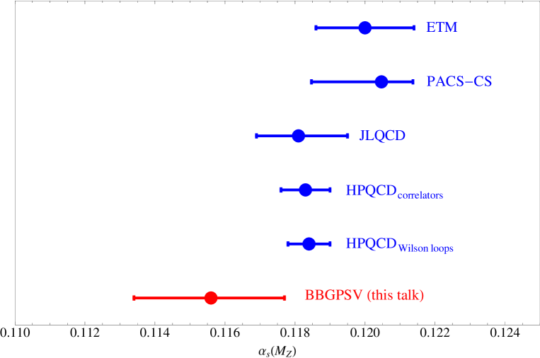
Figure 1: Comparison of our result for $\alpha_{s}(M_{Z})$ with other recent lattice determinations. The references are: HPQCD [23], JLQCD [25], PACS-CS [26], ETM [27].

In Fig. 2 we compare our result for $\alpha_{s}(M_{Z})$ in Eq. (5) with a few other recent $\alpha_{s}$ determinations that use other techniques (i.e. non-lattice determinations);

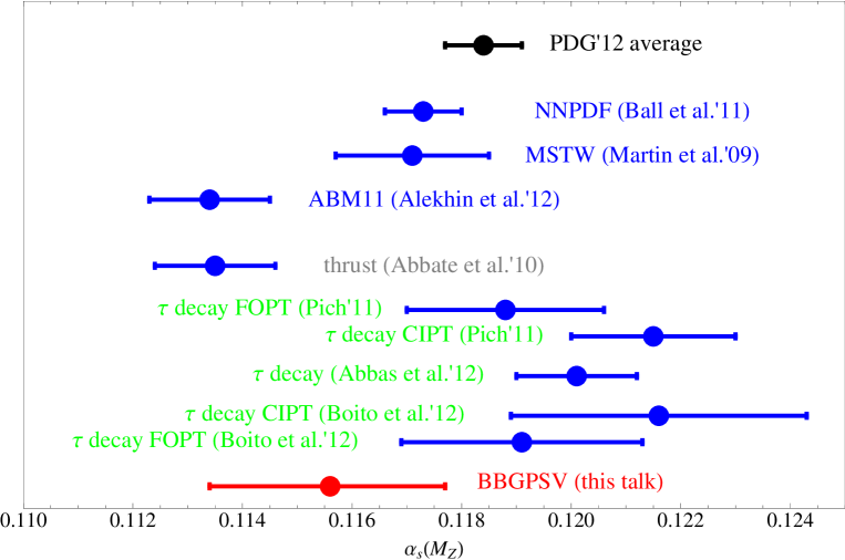
Figure 2: Comparison of our result for $\alpha_{s}(M_{Z})$ with a few other recent $\alpha_{s}$ determinations. We include results from $\tau$ decays (Boito et al. [28]; Abbas et al. [29]; Pich [30]), thrust (Abbate et al. [31]), and PDF fits (ABM11 [32], MSTW [33], NNPDF [34]), along with the PDG average [35] for reference.

we include results coming from $\tau$ decays, thrust, and parton distribution function (PDF) fits, along with the Particle Data Group (PDG) average (the comparison is not exhaustive, we just show a few other recent results in the figure, meant to illustrate where our result lay with respect to recent $\alpha_{s}$ extractions).

It is also worth remarking that our $\alpha_{s}$ determination is performed at a scale of around 1.5 GeV, and therefore constitutes an important new ingredient to further test the running of the strong coupling (see Fig. 2 of Ref. [1] for a graphical comparison of different determinations of $\alpha_{s}$ as a function of the energy scale $Q$ where they are performed).

5 Conclusions

To summarize, in this work we have compared perturbative calculations for the QCD static energy at short distances with lattice computations. We find that perturbation theory (after canceling the leading renormalon singularity) is able to describe the short-distance part of the static energy computed in $2+1$ flavor lattice QCD (see Fig. 1 of Ref. [1] for a comparison of the different orders of accuracy of the perturbative result and the lattice data). We exploited this fact to obtain a determination of the strong coupling $\alpha_{s}$. Our extraction is at three-loop accuracy (including resummation of the leading ultrasoft logarithms) and is performed at a scale of 1.5 GeV. When we evolve the result to the scale $M_{Z}$ it corresponds to $\alpha_{s}\left(M_{Z}\right)=0.1156^{+0.0021}_{-0.0022}$.

- [1] A. Bazavov, N. Brambilla, X. Garcia i Tormo, P. Petreczky, J. Soto and A. Vairo, arXiv:1205.6155 [hep-ph].
- [2] N. Brambilla, X. Garcia i Tormo, J. Soto and A. Vairo, Phys. Rev. Lett. 105, 212001 (2010) [arXiv:1006.2066 [hep-ph]].
- [3] A. Pineda and M. Stahlhofen, Phys. Rev. D 84, 034016 (2011) [arXiv:1105.4356 [hep-ph]].
- [4] A. V. Smirnov, V. A. Smirnov and M. Steinhauser, Phys. Rev. Lett. 104, 112002 (2010) [arXiv:0911.4742 [hep-ph]].
- [5] C. Anzai, Y. Kiyo and Y. Sumino, Phys. Rev. Lett. 104, 112003 (2010) [arXiv:0911.4335 [hep-ph]].
- [6] N. Brambilla, X. Garcia i Tormo, J. Soto and A. Vairo, Phys. Rev. D 80, 034016 (2009) [arXiv:0906.1390 [hep-ph]].
- [7] A. V. Smirnov, V. A. Smirnov and M. Steinhauser, Phys. Lett. B 668, 293 (2008) [arXiv:0809.1927 [hep-ph]].
- [8] N. Brambilla, X. Garcia i Tormo, J. Soto and A. Vairo, Phys. Lett. B 647, 185 (2007) [hep-ph/0610143].
- [9] T. Appelquist, M. Dine and I. J. Muzinich, Phys. Rev. D 17, 2074 (1978).
- [10] N. Brambilla, A. Pineda, J. Soto and A. Vairo, Phys. Rev. D 60, 091502 (1999) [hep-ph/9903355].
- [11] X. Garcia i Tormo, arXiv:1208.4850 [hep-ph].
- [12] A. Bazavov, T. Bhattacharya, M. Cheng, C. DeTar, H. T. Ding, S. Gottlieb, R. Gupta and P. Hegde et al., Phys. Rev. D 85, 054503 (2012) [arXiv:1111.1710 [hep-lat]].
- [13] E. Follana et al. [HPQCD and UKQCD Collaborations], Phys. Rev. D 75, 054502 (2007) [hep-lat/0610092].
- [14] R. Sommer, Nucl. Phys. B 411, 839 (1994) [hep-lat/9310022].
- [15] C. Aubin, C. Bernard, C. DeTar, J. Osborn, S. Gottlieb, E. B. Gregory, D. Toussaint and U. M. Heller et al., Phys. Rev. D 70, 094505 (2004) [hep-lat/0402030].
- [16] S. Necco and R. Sommer, Nucl. Phys. B 622, 328 (2002).
- [17] S. P. Booth et al. [UKQCD Collaboration], Nucl. Phys. B 394, 509 (1993) [hep-lat/9209007].
- [18] M. Beneke, Phys. Lett. B 434 (1998) 115 [hep-ph/9804241].
- [19] A. H. Hoang, M. C. Smith, T. Stelzer and S. Willenbrock, Phys. Rev. D 59, 114014 (1999) [hep-ph/9804227].
- [20] A. Pineda, JHEP 0106 (2001) 022 [hep-ph/0105008].
- [21] K. G. Chetyrkin, J. H. Kuhn and M. Steinhauser, Comput. Phys. Commun. 133, 43 (2000) [hep-ph/0004189].
- [22] C. T. H. Davies et al. [HPQCD Collaboration], Phys. Rev. D 78, 114507 (2008) [arXiv:0807.1687 [hep-lat]].
- [23] C. McNeile, C. T. H. Davies, E. Follana, K. Hornbostel and G. P. Lepage, Phys. Rev. D 82, 034512 (2010) [arXiv:1004.4285 [hep-lat]].
- [24] I. Allison et al. [HPQCD Collaboration], Phys. Rev. D 78, 054513 (2008) [arXiv:0805.2999 [hep-lat]].
- [25] E. Shintani, S. Aoki, H. Fukaya, S. Hashimoto, T. Kaneko, T. Onogi and N. Yamada, Phys. Rev. D 82, 074505 (2010) [arXiv:1002.0371 [hep-lat]].
- [26] S. Aoki et al. [PACS-CS Collaboration], JHEP 0910, 053 (2009) [arXiv:0906.3906 [hep-lat]].
- [27] B. Blossier, P. Boucaud, M. Brinet, F. De Soto, X. Du, V. Morenas, O. Pene and K. Petrov et al., arXiv:1201.5770 [hep-ph].
- [28] D. Boito, M. Golterman, M. Jamin, A. Mahdavi, K. Maltman, J. Osborne and S. Peris, Phys. Rev. D 85, 093015 (2012) [arXiv:1203.3146 [hep-ph]].
- [29] G. Abbas, B. Ananthanarayan and I. Caprini, Phys. Rev. D 85, 094018 (2012) [arXiv:1202.2672 [hep-ph]].
- [30] S. Bethke, A. H. Hoang, S. Kluth, J. Schieck, I. W. Stewart, S. Aoki, M. Beneke and S. Bethke et al., arXiv:1110.0016 [hep-ph].
- [31] R. Abbate, M. Fickinger, A. H. Hoang, V. Mateu and I. W. Stewart, Phys. Rev. D 83, 074021 (2011) [arXiv:1006.3080 [hep-ph]].
- [32] S. Alekhin, J. Blumlein and S. Moch, Phys. Rev. D 86, 054009 (2012) [arXiv:1202.2281 [hep-ph]].
- [33] A. D. Martin, W. J. Stirling, R. S. Thorne and G. Watt, Eur. Phys. J. C 64, 653 (2009) [arXiv:0905.3531 [hep-ph]].
- [34] R. D. Ball, V. Bertone, L. Del Debbio, S. Forte, A. Guffanti, J. I. Latorre, S. Lionetti and J. Rojo et al., Phys. Lett. B 707, 66 (2012) [arXiv:1110.2483 [hep-ph]].
- [35] J. Beringer et al. [Particle Data Group Collaboration], Phys. Rev. D 86, 010001 (2012).