Smoothing Dynamic Systems with State-Dependent Covariance Matrices

Abstract

Kalman filtering and smoothing algorithms are used in many areas, including tracking and navigation, medical applications, and financial trend filtering. One of the basic assumptions required to apply the Kalman smoothing framework is that error covariance matrices are known and given. In this paper, we study a general class of inference problems where covariance matrices can depend functionally on unknown parameters. In the Kalman framework, this allows modeling situations where covariance matrices may depend functionally on the state sequence being estimated. We present an extended formulation and generalized Gauss-Newton (GGN) algorithm for inference in this context. When applied to dynamic systems inference, we show the algorithm can be implemented to preserve the computational efficiency of the classic Kalman smoother. The new approach is illustrated with a synthetic numerical example.

I Introduction

The Kalman filter [16] and smoother [19] are efficient algorithms to estimate the state of a dynamic system given noisy measurements. Over the last 10 years, the optimization perspective on the smoothing problem has produced many extensions to dynamic system estimation, including methods for smoothing systems with nonlinear process and measurement models [8], systems with nonlinear inequality constraints [10], robust Kalman smoothing [6, 5, 4], and smoothing of sparse systems [1].

In all of the above extensions, the variances of process and measurement errors are assumed to be fixed and known. In practice, these quantities are often not known, and may in fact depend on the state. For example, radar position errors are known to depend on the aspect angle as well as the position of the target [21]. In some applications [17], it may be of interest to do Kalman filtering in polar coordinates or other coordinates that induce a state dependence in measurement errors. Modeling of process error covariance may also be state dependent — for example, Bar-Shalom [7] suggests that the right choice of process noise level for flight tracking models depends on the turn rate range expected. Therefore if we are estimating turn rate as part of the state, the process noise level can be modeled as a function of (a portion of) the state.

These ideas motivate extensions of the standard Kalman smoothing formulation to situations where process and measurement variances have known functional dependence on the state. Several such extensions have already been considered. In [21], the Unscented Transform is used to fit models with state-dependent matrices acting on observation noise. Linear systems with additive observation noise where measurement error variance is a known function of the state are studied in [22]. Linear systems with control inputs transformed by state-dependent matrices are considered in [14]. Finally, adaptive system identification, as presented in [13], also falls into this class.

In this paper, we formulate the state-dependent covariance problem as a statistical estimation problem, and develop algorithms for obtaining the maximum a posteriori (MAP) estimate. The ideas presented here extend those developed in [11] for diagonal covariance matrices in kinetic tracer studies. In the theoretical development, we allow the process and measurement functions to be nonlinear, and we allow the functional dependence of covariance on the state to be nonlinear as well.

The paper proceeds as follows. In Section II, we review the statistical origins of the Kalman smoother, casting it as a structured nonlinear regression problem. We show that consideration of state-dependent variance in such a regression brings to the forefront terms that are usually ignored, and develop an extended MAP objective to optimize. The proposed formulation can be used for general nonlinear regression where variance depends in a known functional way on the parameters. In Section III we build a new algorithm for solving the resulting optimization problems, exploiting their convex composite structure. The key step is a special convex subproblem, which we solve in Section IV. In Section V, we show the necessary details required to implement this method for time series analysis, so as to preserve the computational complexity of the classic smoothing algorithms. In Section VI, we provide a numerical experiment using simulated data that demonstrates the performance of the new smoother and the potential modeling capabilities of the approach. We end with conclusions.

II Kalman Smoothing with State-Dependent Uncertainty

The dynamic structure of the Kalman smoothing problem is specified as follows:

$$\begin{array}[]{rcll}{\bf x_{1}}&=&g_{1}(x_{0})+{\bf w_{1}},\\ {\bf x_{k}}&=&g_{k}({\bf x_{k-1}})+{\bf w_{k}}&k=2,\ldots,N,\\ {\bf z_{k}}&=&h_{k}({\bf x_{k}})+{\bf v_{k}}&k=1,\ldots,N\;,\end{array}$$ (1)

where $g_{k},h_{k}$ are known (nonlinear) process and measurement functions, and ${\bf w_{k}}\in{\mathbb{R}}^{n}$, ${\bf v_{k}}\in{\mathbb{R}}^{m(k)}$ are mutually independent Gaussian random variables with positive definite covariance matrices $Q_{k}$ and $R_{k}$, ${\bf x_{k}}\in{\mathbb{R}}^{n}$ are the unknown states, and ${\bf z_{k}}\in{\mathbb{R}}^{m(k)}$ are the observed measurements.

Considering model (1) and using Bayes’ theorem, the conditional likelihood of the entire state sequence $\{x_{k}\}$ given the measurement sequence $\{z_{k}\}$ is given by

$${\bf p}\left(\{x_{k}\}\big{|}\{z_{k}\}\right)\propto{\bf p}\left(\{z_{k}\}\big{|}\{x_{k}\}\right){\bf p}\left(\{x_{k}\}\right)\;,$$ (2)

which in turn can be written in terms of the likelihood of state increments ${\bf p}(w_{k})$ and measurement residuals ${\bf p}(v_{k})$:

$${\bf p}\left(\{z_{k}\}\big{|}\{x_{k}\}\right){\bf p}\left(\{x_{k}\}\right)=\kappa\prod_{k=1}^{N}{\bf p}(v_{k}){\bf p}(w_{k})$$ (3)

$$=\kappa\prod_{k=1}^{N}\exp\Big{(}-\frac{1}{2}(z_{k}-h_{k}(x_{k}))^{\top}R_{k}^{-1}(z_{k}-h_{k}(x_{k}))$$

$$\quad\quad-\frac{1}{2}(x_{k}-g_{k}(x_{k-1}))^{\top}Q_{k}^{-1}(x_{k}-g_{k}(x_{k-1}))\Big{)}\;,$$

where we define $g_{1}(x_{0})=x_{0}$. The constant of proportionality $\kappa$ is usually ignored, since in classic models, the variance terms $Q_{k}$ and $R_{k}$ are fixed. It is given by

$$\kappa=\prod_{k=1}^{n}\frac{1}{(2\pi)^{n/2}\det(Q_{k})}\frac{1}{(2\pi)^{m(k)/2}\det(R_{k})}.$$ (4)

Our main contribution here is to remove the assumption that $Q_{k}$ and $R_{k}$ are fixed and known, and instead model these covariance matrices as known $\mathcal{C}^{2}$ functions of the state. In this setting, $\kappa$ in (4) is no longer a constant, and must be accounted for. To design our approach, we assume that we are given the inverse Cholesky factors $Q_{k}^{-1/2}(x_{k})$ and $R_{k}^{-1/2}(x_{k})$ as functions of the state. For simple (e.g. diagonal variance) models, there is no loss of generality here; one can easily transform between different representations. When $Q_{k}$ and $R_{k}$ are full, however, the assumption that inverse Cholesky factors are available is essential for our approach. In addition to considerations of computational efficiency, the main motivation behind the assumption is the selection of an appropriate convex-composite model; this is explained in detail in the next section.

In order to develop a simpler notation for estimating the entire state sequence, we define functions $g:\mathbb{R}^{nN}\rightarrow\mathbb{R}^{nN}$ and $h:\mathbb{R}^{nN}\rightarrow\mathbb{R}^{M}$, with $M=\sum_{k}m_{k}$, from components $g_{k}$ and $h_{k}$ as follows:

$$g(x)=\begin{bmatrix}x_{1}\\ x_{2}-g_{2}(x_{1})\\ \vdots\\ x_{N}-g_{N}(x_{N-1})\end{bmatrix}\;,\quad h(x)=\begin{bmatrix}h_{1}(x_{1})\\ h_{2}(x_{2})\\ \vdots\\ h_{N}(x_{N})\end{bmatrix}\;.$$ (5)

Given a sequence of column vectors $\{u_{k}\}$ and matrices $\{T_{k}\}$ we use the following notation:

$${\rm vec}(\{u_{k}\})=\begin{bmatrix}u_{1}\\ u_{2}\\ \vdots\\ u_{N}\end{bmatrix}\;,\;{\rm diag}(\{T_{k}\})=\begin{bmatrix}T_{1}&0&\cdots&0\\ 0&T_{2}&\ddots&\vdots\\ \vdots&\ddots&\ddots&0\\ 0&\cdots&0&T_{N}\end{bmatrix},$$ (6)

$$\begin{aligned} R&={\rm diag}(\{R_{k}\})\\ Q&={\rm diag}(\{Q_{k}\})\\ x&={\rm vec}(\{x_{k}\})\end{aligned}\quad\quad\quad\begin{aligned} w&={\rm vec}(\{g_{0},0,\dots,0\})\\ z&={\rm vec}(\{z_{1},\dots,z_{N}\})\\ g_{0}&=g_{1}(x_{0}).\end{aligned}$$

With this notation, and under Gaussian assumptions, the extended MAP object for the Kalman smoother, which incorporates state-dependent variance terms, is given by

$$\frac{1}{2}\|Q^{-1/2}(x)(g(x)-w)\|_{2}^{2}+\frac{1}{2}\|R^{-1/2}(x)(h(x)-z)\|_{2}^{2}$$ (7)

$$-\log\det\left(Q^{-1/2}(x)\right)-\log\det\left(R^{-1/2}(x)\right)\;.$$

With (7) in front of us, we see why the log determinant terms play an important role. Without these terms, an optimization approach to minimize a weighted sum of squares will aim to drive $Q^{-1/2}(x)$ and $R^{-1/2}(x)$ to $0$ if at all possible. The function $-\log(\cdot)$ acts as a barrier to prevent this from happening.

III Convex Composite Formulation and Algorithm

We would like to apply the generalized Gauss-Newton methodology for minimizing convex composite functions [12] to the objective (7). The first step in this process is to write this objective in convex composite form, that is, in the form $f=\rho\circ F$, where $\rho$ is convex and $F$ is smooth. The choice of the functions $\rho$ and $F$ depend on how we wish to model the representation of the problem. The most straightforward way to rewrite (7) is the more general form

$$J(x):=\frac{1}{2}c(x)^{T}W(x)^{-1}c(x)+\frac{1}{2}\log\det(W(x)),$$

where $c\,:\,{\mathbb{R}}^{nN}\rightarrow{\mathbb{R}}^{M+nN}$ and $W\,:\,{\mathbb{R}}^{nN}\rightarrow\mathcal{S}^{M+nN}_{++}$ are smooth maps given by

$$c(x)=\begin{bmatrix}x_{1}-g_{0}\\ h_{1}(x_{1})-z_{1}\\ x_{2}-g_{2}(x_{1})\\ h_{2}(x_{2})-z_{2}\\ \vdots\\ x_{N}-g_{N}(x_{N-1})\\ h_{N}(x_{N})-z_{N}\end{bmatrix},$$ (8)

$$W(x)=\begin{bmatrix}Q_{1}(x_{1})&0&&&\\ 0&R_{1}(x_{1})&&&\\ \vdots&\ddots&\ddots&&\vdots\\ &&&Q_{N}(x_{N})&0\\ &&&0&R_{N}(x_{N})\end{bmatrix}$$ (9)

where $\mathcal{S}^{M+nN}_{++}$ is the cone of real symmetric $({M+nN})\times({M+nN})$ positive definite matrices.

Then $J=\hat{\rho}\circ\hat{F}$ with

$$\hat{\rho}(c,W) :=\frac{1}{2}c^{T}W^{-1}c+\frac{1}{2}\log\det(W)$$

$$\hat{F}(x) =(c(x),W(x)).$$

Although the function $\hat{F}$ in this formulation can be assumed smooth, the function $\hat{\rho}$ is not convex. Indeed, $\hat{\rho}$ is the difference of two convex functions. When viewed as a function of $(c,W^{-1})$, it is still not jointly convex in these arguments.

Here, we propose an approach that applies in many practical settings and yields an efficient solution procedure. However, a price is paid in a more complex model for the covariance matrices. Specifically, we assume that the Cholesky factors for $Q_{k}^{-1}(x_{k})$ and $R_{k}^{-1}(x_{k})$ are given to us as explicit functions of the state. We denote these factors by $Q_{k}^{-1/2}(x_{k})$ and $R_{k}^{-1/2}(x_{k})$, respectively. In some settings, the matrices $Q_{k}(x_{k})$ and $R_{k}(x_{k})$ are modeled as diagonal matrices, in which case the inverse Cholesky factors are easily computed diagonal matrices. We provide an example of this type in the final section. Under this modeling assumption, the objective (7) can be abstracted to the more general form

$$K(x)=\frac{1}{2}c(x)^{\rm T}V(x)^{T}V(x)c(x)-\log\circ\det[V(x)]\;,$$ (10)

where $c\,:\,{\mathbb{R}}^{nN}\rightarrow{\mathbb{R}}^{M+nN}$ is exactly as in (8) and $V\,:\,{\mathbb{R}}^{nN}\rightarrow\mathcal{L}^{M+nN}$ is given by

$$V(x)=\begin{bmatrix}Q_{1}^{-1/2}&0&&&\\ 0&R_{1}^{-1/2}&&&\\ \vdots&\ddots&\ddots&&\vdots\\ &&&Q_{N}^{-1/2}&0\\ &&&0&R_{N}^{-1/2}\end{bmatrix},$$ (11)

where all blocks of V are functions of $x$, and $\mathcal{L}^{M+nN}$ is the subalgebra of $({M+nN})\times({M+nN})$ real lower triangular matrices. Throughout, we assume that both $c$ and $V$ are twice continuously differentiable and that $\mathrm{dom}(K):=\left\{x\,\left|\,K(x)<+\infty\right.\right\}=\left\{x\,\left|\,V(x)\in\mathcal{L}^{M+nN}_{++}\right.\right\}\neq\emptyset$, where $\mathcal{L}^{M+nN}_{++}$ is the cone of $({M+nN})\times({M+nN})$ real lower triangular matrices with strictly positive entries on the diagonal. Now $K$ can be written in convex composite form $K(x)=\rho\circ F$ with

$$\rho(u,v) = \frac{1}{2}u^{\rm T}u-\sum_{i}\log[v_{i}]$$ (12)

$$\quad F(x) = \begin{bmatrix}F_{1}(x)\\ F_{2}(x)\\ \end{bmatrix}=\begin{bmatrix}V(x)c(x)\\ {\rm vec}[\{V_{ii}(x)\}]\end{bmatrix}\;.$$ (13)

Note that $\mathrm{dom}(\rho)={\mathbb{R}}^{M+nN}\times{\mathbb{R}}^{M+nN}_{++}$.

The direction finding subproblem in a Gauss-Newton method takes the form

$$\min_{d}\rho(F(x)+F^{\prime}(x)d)+\mbox{\small$\frac{\omega}{2}$}d^{\rm T}d\ ,$$

for some $\omega\geq 0$. The quadratic term $\frac{\omega}{2}d^{\rm T}d$ is a regularization term that both guarantees the uniqueness of the solution and regulates its magnitude. The convergence analysis of methods of this type rely heavily on the difference function

$$\Delta(x;d)=\rho\left(\;F(x)+F^{\prime}(x)d\;\right)-K(x)\;.$$ (14)

which is important for both convergence criteria and the line search in the overall method. In particular, [12, Lemma 2.3]

$$K^{\prime}(x:d)=\inf_{t>0}t^{-1}\Delta(x;td)\mbox{ for all }d\in{\mathbb{R}}^{nN},\;x\in\mathrm{dom}(K)$$ (15)

since, whenever $F_{2}(x)>0$, then, for all $d$, $F_{2}(x)+F^{\prime}_{2}(x)(td)>0$ for all $t$ sufficiently small.

Linearizing the functions $F_{i}(x)$ in (12) yields approximations $\tilde{F}_{i}(x;d):=F_{i}(x)+F^{\prime}_{i}(x)d$, which in turn gives the approximation

$$\tilde{K}(x;d)=\rho[\tilde{F}_{1}(x;d),\tilde{F}_{2}(x;d)]\;.$$ (16)

This is the objective for the direction finding subproblem. Here,

$$\begin{array}[]{lll}\tilde{F}_{1}(x;d)&=&\left(V(x)\partial_{x}c(x)+(c(x)^{\rm T}\otimes I_{N})\partial_{x}V(x)\right)d\\ &&\quad+V(x)c(x)\\ \tilde{F}_{2}(x;d)&=&{\rm vec}\left(\{V_{ii}(x)+\partial_{x}V_{ii}(x)d\}\right).\end{array}$$ (17)

Note that we must be sure that $\tilde{F}_{2}(x;d)$ is component-wise greater than zero. For details of these derivations, see [2]. The Gauss-Newton subproblem is now given by

$${\bar{\Delta}}(x):=\min_{d\in{\mathbb{R}}^{nN}}\Delta(x;d)+\mbox{\small$\frac{\omega}{2}$}d^{\rm T}d$$ (18)

$$=\min_{d\in{\mathbb{R}}^{nN}}\frac{1}{2}\tilde{F}_{1}(x;d)^{\rm T}\tilde{F}_{1}(x;d)+\mbox{\small$\frac{\omega}{2}$}d^{\rm T}d-\sum_{i}\log[\tilde{F}_{2}(x;d)]\;.$$

Due to our assumptions on $c$ and $V$, these subproblems are always well defined, are convex, and have a unique solution which must always exist. In addition, they provide an estimate for the first-order optimality for $K$.

Theorem III.1

[12, Theorem 3.6] Let $x\in\mathrm{dom}(K)$. Then the following three statements are equivalent:

1. ${\bar{\Delta}}(x)=0$,

2. $\bar{d}=0$ solves (18), and

3. $0\in\partial K(x)$, where $\partial K(x)=F^{\prime}(x)^{T}\partial\rho(F(x))$ is the generalized subdifferential of $K$ at $x$ [20, Definition 8.3].

In particular, these conditions imply that $x$ is a first-order stationary point for $K$.

If we ignore dependence on $x$, the optimization problem in (18) can be rewritten as

$$\min_{d\in{\mathbb{R}}^{nN}} \frac{1}{2}d^{\rm T}Cd+a^{\rm T}d-\sum_{i}\log[s_{i}]$$ (19)

s.t. $$\quad s={\rm vec}\{V_{ii}\}+\partial_{x}{\rm vec}\{V_{ii}\}d,$$

where

$$C =\omega I+\widetilde{V}^{\rm T}\widetilde{V}$$ (20)

$$a =\widetilde{V}^{\rm T}Vc$$

$$\widetilde{V} =[V\partial_{x}c\!+\!(c^{\rm T}\otimes I_{N})\partial_{x}V]$$

Note that $a$ is the gradient of the quadratic portion of the extended objective with respect to the state sequence $x$. The quantity $(c^{\rm T}\otimes I_{N})\partial_{x}V$ that appears in (20) can be rewritten as

$$\begin{array}[]{lll}(c^{\rm T}\otimes I_{N})\partial_{x}V&=&\sum_{i=1}^{M+nN}c_{i}\partial_{x}V_{i\cdot}\ .\end{array}$$ (21)

The Lagrangian associated with the extended subproblem (19) is given by

$$L(d,s,\lambda) =\frac{1}{2}d^{\rm T}Cd+a^{\rm T}d-\sum_{i}\log[s_{i}]$$ (22)

$$+\lambda^{\rm T}\left(s-{\rm vec}\{V_{ii}\}-\partial_{x}{\rm vec}\{V_{ii}\}d\right),$$

for $s>0$ and $\lambda>0$. The corresponding optimality conditions state that a direction $d$ solves (19) if and only if there exist $s,\lambda\in{\mathbb{R}}^{M+nN}_{++}$ such that

$$\begin{array}[]{lll}\nabla_{d}L&=&Cd+a-\partial_{x}{\rm vec}\{V_{ii}\}^{\rm T}\lambda=0\\ \nabla_{s}L&=&-D(s)^{-1}{\bf 1}+\lambda=0\\ \nabla_{\lambda}L&=&s-{\rm vec}\{V_{ii}\}-\partial_{x}{\rm vec}\{V_{ii}\}d=0\;,\end{array}$$ (23)

where $D(s):=\mathrm{diag}(s)$.

We refer to (19) as the extended subproblem. In the next section, we show that this problem can be rapidly solved. This motivates the Extended Gauss-Newton method for (10).

Algorithm III.1

Generalized Gauss-Newton Algorithm.

The inputs to this algorithm are

• $x^{0}\in\mathrm{dom}(K):=\{x:K(x)<\infty\}\subset{\mathbb{R}}^{Nn}$: initial estimate of state sequence

• $\varepsilon\geq 0$: overall termination criterion

• $\omega>0$: regularization parameter

• $\beta\in(0,1)$: step size selection parameter

• $\gamma\in(0,1)$: line search step size factor

The steps are as follows:

1. Set the iteration counter $\nu=0$.

2. (Generalized Gauss-Newton Step)

   Find descent direction $d^{\nu}$ solving (19) and set $\Delta_{\nu}:={\bar{\Delta}}(x^{\nu})=\Delta(x^{\nu};d^{\nu})$. Terminate if $\Delta_{\nu}\geq-\varepsilon$.

3. (Line Search) Set

   $$\begin{array}[]{lll}t_{\nu}&=&\max\gamma^{i}\\ &\text{s.t.}&i\in\{0,1,2,\cdots\}\;\mbox{ and }\\ &\text{s.t.}&\rho\left(F(x^{\nu}+\gamma^{i}d^{\nu})\right)\leq\rho\left(F(x^{\nu})\right)+\beta\gamma^{i}\Delta_{\nu}.\end{array}$$

4. (Iterate) Set $x^{\nu+1}=x^{\nu}+t_{\nu}d^{\nu}$ and return to Step 2.

Remark III.2

Note that the line search is well defined whenever $\Delta_{\nu}\neq 0$. Indeed, since whenever $\mathrm{diag}(V(x))>0$, then, for all $d$, $F_{2}(x;td)>0$ for all $t$ sufficiently small. Consequently, since $x^{0}\in\mathrm{dom}(K)$, we have $\{x^{\nu}\}\subset\mathrm{dom}(K)$. In addition, by (15), $K^{\prime}(x^{\nu};d^{\nu})\leq\Delta_{\nu}<{\bar{\Delta}}(x^{\nu})$, so that $\gamma^{-i}\Delta(x^{\nu};\gamma^{i}d^{\nu})<\beta\Delta_{\nu}$ for all $i$ sufficiently large.

Theorem III.2

[Convergence] Let $\{x^{\nu}\}$ be generated by Algorithm III.1 with $\epsilon=0$. Then either the algorithm terminates finitely at a first-order stationary point for $K$ or the sequence $\{x^{\nu}\}$ is infinite and every cluster point of the sequence is a first-order stationary point for $K$.

The proof is given in the appendix.

In the next section, we show how to solve the subproblem (19) for a general state-dependent covariance regression problem.

IV Solving the Extended Subproblem

To solve the direction finding subproblem, we apply a damped Newton method directly to the optimality conditions (23). We present the high-level method here, with details concerning Kalman smoothing given in the next section.

Let $E(s,\lambda,d)$ denote the KKT system given in (23), rearranged in a particular order:

$$E(s,\lambda,d)=\begin{bmatrix}s-{\rm vec}\{V_{ii}\}-\partial_{x}{\rm vec}\{V_{ii}\}d\\ D(s)D(\lambda){\bf 1}-{\bf 1}\\ Cd+a-\partial_{x}{\rm vec}\{V_{ii}\}^{\rm T}\lambda\end{bmatrix}\\$$ (24)

Our goal is to find $(\overline{s},\overline{\lambda},\overline{d})$ for which $E(\overline{s},\overline{\lambda},\overline{d})=0$. We use damped Newton’s method on E which requires solving the Newton equation

$$\nabla E(s,\lambda,d)\begin{bmatrix}\Delta s\\ \Delta\lambda\\ \Delta d\end{bmatrix}=-E(s,\lambda,d),$$ (25)

where $\nabla E(s,\lambda,d)$ is given by

$$\begin{bmatrix}I&0&-\partial_{x}{\rm vec}\{V_{ii}\}\\ D(\lambda)&D(s)&0\\ 0&-\partial_{x}{\rm vec}\{V_{ii}\}^{\rm T}&C\end{bmatrix}.$$ (26)

Define

$${\mathcal{V}}=\partial_{x}{\rm vec}\{V_{ii}\}.$$

Then, using row operations

$$R_{2} =R_{2}-D(\lambda)R_{1}$$

$$R_{3} =R_{3}+{\mathcal{V}}^{\rm T}D(s)^{-1}R_{2},$$

we obtain the modified system

$$\begin{array}[]{lll}&&\begin{bmatrix}I&0&-{\mathcal{V}}\\ 0&D(s)&D(\lambda){\mathcal{V}}\\ 0&0&\Phi\end{bmatrix}\begin{bmatrix}\Delta s\\ \Delta\lambda\\ \Delta d\end{bmatrix}=\begin{bmatrix}\alpha\\ \beta\\ \gamma\end{bmatrix}\;,\end{array}$$ (27)

where

$$\Phi=C+{\mathcal{V}}^{\rm T}D(s)^{-1}D(\lambda){\mathcal{V}}$$ (28)

and

$$\begin{array}[]{lll}\alpha&=&-s+{\rm vec}\{V_{ii}\}+{\mathcal{V}}d\\ \beta&=&{\bf 1}-D(\lambda)\left({\rm vec}\{V_{ii}\}+{\mathcal{V}}d\right)\\ \gamma&=&{\mathcal{V}}^{\rm T}\Big{(}\lambda+D(s)^{-1}\left({\bf 1}-D(\lambda)({\rm vec}\{V_{ii}\}+{\mathcal{V}}d)\right)\Big{)}\\ &&-Cd-a\;.\end{array}$$

By (20), the matrix $C$ is always positive definite and so $\Phi$ is always positive definite and hence invertible. This allows us to recover the Newton direction:

$$\begin{array}[]{lll}\Delta d&=&\Phi^{-1}\gamma\\ \Delta\lambda&=&D(s)^{-1}\Big{(}{\bf 1}-D(\lambda)({\rm vec}\{V_{ii}\}+{\mathcal{V}}(d+\Delta d))\Big{)}\\ \Delta s&=&-s+{\rm vec}\{V_{ii}\}+{\mathcal{V}}(d+\Delta d)\ .\end{array}$$ (29)

Note that any damping scheme requires that $s>0$ for the objective to be finite, and hence, in addition, we require that $\lambda>0$ since we need $D(s)D(\lambda){\bf 1}={\bf 1}$ .

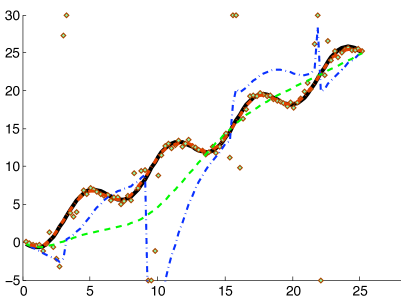
Figure 1: True state $x_{1}$ (black curve), Extended Smoother estimate (thick red dash-dot), Kalman filter estimate (blue dash-dot) and Kalman Smoother estimate (green dashed curve). Measurements are displayed as diamonds, and those outside the axis range are displayed on the figure boundary.

V Structure of the Extended Kalman Smoothing Objective

We now specify the method in the previous section to the Kalman smoothing problem, and demonstrate that the computational efficiency of the Kalman smoother can be preserved.

The functions $c(x)$ and $V(x)$ are given by (8) and (11).

With these definitions, objective $K(x)$ in (10) is exactly (7), and can be written explicitly as follows:

$$\begin{array}[]{lll}&&\frac{1}{2}\Big{(}c^{\rm T}(x)V(x)^{\rm T}V(x)c(x)\Big{)}-\log\circ\det[V(x)]\\ &=&\displaystyle\frac{1}{2}\sum^{N}_{k=1}\|[z_{k}-h_{k}(x_{k})]\|^{2}_{R_{k}^{-T/2}(x_{k})R_{k}^{-1/2}(x_{k})}\\ &&+\displaystyle\frac{1}{2}\sum^{N}_{k=0}\|x_{k}-g_{k}(x_{k-1})\|^{2}_{Q_{k}^{-T/2}(x_{k})Q_{k}^{-1/2}(x_{k})}\\ &&-\log\det(R^{-1/2}_{k}(x_{k}))-\log\det(Q^{-1/2}_{k}(x_{k})),\end{array}$$ (30)

where, for any symmetric positive definite matrix $Q$, $\|u\|^{2}_{Q}:=u^{T}Qu$.

We now derive the explicit forms for $C$ and $a$ in (20) for the Gauss-Newton subproblem (19). Recall that $C$ and $a$ are given by

$$C =\!\omega I\!+\![V\partial_{x}c\!+\!(c^{\rm T}\otimes I_{N})\partial_{x}V]^{\rm T}[V\partial_{x}c\!+\!(c^{\rm T}\otimes I_{N})\partial_{x}V],$$

$$a =\!c^{\rm T}V^{\rm T}V\partial_{x}c+c^{\rm T}V^{\rm T}(c^{\rm T}\otimes I_{N})\partial_{x}V.$$

where

$$\begin{array}[]{lll}(c^{\rm T}\otimes I_{N})\partial_{x}V&=&\sum_{i=1}^{M+nN}c_{i}\partial_{x}V_{i\cdot},\end{array}$$

and

$$\partial_{x}c(x)=\begin{bmatrix}{\rm I}&0&&&\\ H_{1}&0&&\dots&0\\ -G_{2}&{\rm I}&&\ddots&\\ 0&H_{2}&0&&\dots\\ &-G_{3}&\ddots&&0\\ &&\ddots&H_{N-1}&0\\ &&&-G_{N}&{\rm I}\\ &&&0&H_{N}\end{bmatrix}\;,$$ (31)

with $G_{k}=\partial_{x_{k}}g_{k+1}(x_{k})$, $H_{k}=\partial_{x_{k}}h_{k}(x_{k})$, and the dependence on $x$ has been suppressed to decrease the notational burden. Note that the matrix $G$ is invertible, and so $\partial_{x}c(x)$ is injective, that is, $\mathrm{Null}(\partial_{x}c(x))=\{0\}$. In addition, since, we require ${\rm vec}\{V_{ii}\}>0$ at every iteration, the matrix $V^{T}V$ is always positive definite. Consequently, the matrix $\partial_{x}c^{T}V^{T}V\partial_{x}c$ is always positive definite.

Define $\tilde{w}(x)$ and $\tilde{v}(x)$ in (6) by

$$\tilde{w}_{k}(x) = x_{k}-g_{k}(x_{k-1})$$ (32)

$$\tilde{v}_{k}(x) = z_{k}-h_{k}(x_{k})$$ (33)

In the expressions below, we will use notation $\tilde{w}_{k,i}$ to mean the $i$th component of $\tilde{w}_{k}$.

The matrix $(c^{\rm T}\otimes I_{N})\partial_{x}V$ has the following block structure:

$$[(c^{\rm T}\otimes I_{N})\partial_{x}V]=\small\begin{bmatrix}\tilde{Q}_{1}&0&0&0&0&\cdots&0\\ \tilde{R}_{1}&0&0&0&0&\cdots&0\\ 0&\tilde{Q}_{2}&0&0&0&\cdots&0\\ 0&\tilde{R}_{2}&0&0&0&\cdots&0\\ 0&0&0&\ddots&\ddots&\cdots&0\\ 0&0&0&\ddots&\ddots&Q_{N-1}&0\\ 0&0&0&\ddots&\ddots&R_{N-1}&0\\ 0&0&0&\cdots&\cdots&0&\tilde{Q}_{N}\\ 0&0&0&\cdots&\cdots&0&\tilde{R}_{N}\\ \end{bmatrix}$$ (34)

where

$$\tilde{Q}_{i} = \sum_{j=1}^{n}\tilde{w}_{i,j}\partial_{x_{i}}[Q_{i}^{-1/2}]_{j\cdot}$$ (35)

$$\tilde{R}_{i} = \sum_{j=1}^{m(i)}\tilde{v}_{i,j}\partial_{x_{i}}[R_{i}^{-1/2}]_{j\cdot}\;.$$ (36)

Then we can write down the gradient $a$:

$$\begin{array}[]{lll}a&=&\begin{bmatrix}a_{1}^{\rm T}&a_{2}^{\rm T}&\cdots&a_{N}^{\rm T}\end{bmatrix}^{\rm T}\;,\end{array}$$

where

$$\begin{array}[]{lll}a_{j}&=&-\tilde{v}_{j}^{\rm T}R^{-1}_{j}(x_{j})\partial_{x(j)}h_{j}(x_{j})+\tilde{w}_{j}^{\rm T}Q^{-1}_{j}(x_{j-1})\\ &&+\tilde{w}_{j+1}^{\rm T}Q^{-1}_{j+1}(x_{j})\partial_{x(j)}g_{j+1}(x_{j})\\ &&+\tilde{w}_{j}^{\rm T}Q_{j}^{-T/2}\tilde{Q}_{j}+\tilde{v}_{j}^{\rm T}R_{j}^{-T/2}\tilde{R}_{j}\;.\end{array}$$ (37)

Using (31) and (34), we can form

$$\Psi:=V\partial_{x}c+(c^{\rm T}\otimes I_{N})\partial_{x}V,$$

and obtain a closed form solution for $C=\Psi^{T}\Psi$:

$$C =\begin{bmatrix}C_{1}&A^{\rm T}_{2}&0&\\ A_{2}&C_{2}&A^{\rm T}_{3}&0\\ 0&\ddots&\ddots&\ddots\\ &0&A_{N}&C_{N}\end{bmatrix}$$ (38)

$$C_{k} \!=\!\omega I\!+\![Q_{k}^{-1/2}\!\!+\!\tilde{Q}_{k}]^{\rm T}[Q_{k}^{-1/2}\!\!+\!\tilde{Q}_{k}]\!+\!\nabla g_{k+1}^{\rm T}Q_{k+1}^{-1}\!\nabla g_{k+1}$$

$$\ \ +[-R_{k}^{-1/2}\nabla h_{k}+\tilde{R}_{k}]^{\rm T}[-R_{k}^{-1/2}\nabla h_{k}+\tilde{R}_{k}]$$

$$A_{k} =-(Q_{k}^{-1/2}+\tilde{Q}_{k})^{\rm T}Q_{k}^{-1/2}\nabla g_{k}\;.$$

Remark V.1

The matrix (38) is block tridiagonal, and so it can be inverted with effort $O(n^{3}N)$ using any of the algorithms in [9, 3]. The proof sketch is given in the appendix.

Recall the direction finding equation (25) in the Extended GN algorithm:

$$\nabla E(s,\lambda,d)\begin{bmatrix}\Delta s\\ \Delta\lambda\\ \Delta d\end{bmatrix}=-E(s,\lambda,d).$$

The solution to this system is given by (29), with $\Phi$ as in (28), $C$ as in (38), and $[{\mathcal{V}}^{\rm T}D(s)^{-1}D(\lambda){\mathcal{V}}]_{k}$ given by

$$\begin{array}[]{lll}\partial_{x(k)}{\rm diag}\{Q_{k}^{-1/2}\}^{\rm T}D(s_{Q_{k}})^{-1}D(\lambda_{Q_{k}})\partial_{x(k)}{\rm diag}\{Q_{k}^{-1/2}\}\\ +\partial_{x(k)}{\rm diag}\{R_{k}^{-1/2}\}^{\rm T}D(s_{R_{k}})^{-1}D(\lambda_{R_{k}})\partial_{x(k)}{\rm diag}\{R_{k}^{-1/2}\}\;.\end{array}$$

VI Numerical Results

In this section, we present some numerical experiments to show the advantages and modeling possibilities of the new Kalman smoother. The simulation model we consider is similar to the one presented in [10]. The ‘ground truth’ time series for this simulated example is given by

$$x(t)=\begin{bmatrix}1-2\cos(t)\\ t-2\sin(t)\end{bmatrix}\;.$$

The time between measurements is a constant denoted by $\Delta t$. The models for the mean of $x_{k}$ given $x_{k-1}$ and for process covariance $Q_{k}$ [15, 18] are

$$g_{k}(x_{k-1})=\begin{bmatrix}1&0\\ \Delta t&1\end{bmatrix}x_{k-1}\;,\quad Q_{k}=\begin{bmatrix}\Delta t&\Delta t^{2}/2\\ \Delta t^{2}/2&\Delta t^{3}/3\end{bmatrix}.$$

The measurement model for the mean of $z_{k}$ given $x_{k}$ is $h_{k}(x_{k})=x_{2,k}\;,$ where $x_{2,k}$ denotes the second component of $x_{k}$.

The main innovation of the example is in the measurement variance model. The smoother takes inverse Cholesky factors as input, and these are assumed to be $3-x_{1,k}$. Then the variance model is given by $R_{k}(x_{k})=(3-x_{1,k})^{-2}$. The measurements were generated using the measurement model, from two full periods of the time series $x(t)$, with $N=100$ discrete time points equally spaced over the interval $[0,4\pi]$, and with noise sampled from $N(0,R_{k}(x_{k}))$. Since the true state $x_{1}$ varies in the interval $[-1,3]$, the variance for the observations goes to infinity when $t$ is a multiple of $\pi$.

This simulation illustrates a situation where the measurements are very reliable for some state values, but completely unpredictable for others. This phenomenon may occur for example if sensors report garbage values when the attitude of a vehicle is in a particular configuration. The measurement model presented here can be easily adapted by the user to take their beliefs about the system into account. The main point is that as long as the inverse Cholesky factors for the variance can be coded as a smooth function of the state, smoothed estimates for state values can be obtained taking into account this bad behavior of the measurements.

The result of the simulation is shown in Figure 1. The extended Kalman smoother (thick red dash-dot) is able to recover the ground truth (shown in black) with no appreciable difference. The Kalman filter (thin blue dash-dot) is strongly affected by the outlying measurements, as expected. The Kalman smoother (green dashed) is able to smooth the measurements, but cannot pick up the oscillations of the ground truth, which are small in magnitude compared to the size of the errors.

This last point is the most important — it is not just the magnitude of the outliers that makes the Kalman smoother fail, although it can be seen to be rather far off the ground truth. The biggest challenge of the situation presented is knowing which measurements to trust, since this information depends on the state being estimated.

VII Conclusions

In this paper, we presented extended formulations for modeling dynamic systems in cases where the covariance matrices are known functions of the state. The formulation includes variance-control terms arising from statistical modeling assumptions. These terms give rise to an extended convex-composite structure, and we propose a new method, the extended Gauss-Newton, which repeatedly solves extended convex subproblems by exploiting their KKT optimality conditions. When applied to dynamic inference problems, the proposed approach preserves the complexity of the classic Kalman smoother.

VIII Appendix

VIII-A Proof sketch of Remark V.1

Recall the matrix inversion lemma:

Lemma VIII.1 (Matrix Inversion Lemma)

Assume matrices $M_{1}\in\mathbb{R}^{m_{1}\times m_{1}}$ and $M_{2}\in\mathbb{R}^{m_{2}\times m_{2}}$ are symmetric positive definite. Then for any matrix $U\in\mathbb{R}^{m_{1}\times m_{2}}$, the following matrix is also symmetric positive definite:

$$S=M_{1}^{-1}-M_{1}^{-1}U(M_{2}+U^{T}M_{1}^{-1}U)^{-1}U^{T}M_{1}^{-1}.$$ (39)

From this, we get an immediate and useful corollary:

Corollary VIII.2

For a positive definite matrix $M_{2}$, and any matrix $U$, we have

$$\|U^{T}(M_{2}+UU^{T})^{-1}U\|_{2}<1,$$

where $\|\cdot\|_{2}$ denotes the spectral norm.

Simply take $M_{1}=I$ in lemma VIII.1. The conclusion of the lemma gives the result.

Corollary VIII.2 can be applied to show that the algorithms in [3] yield invertible blocks at every iteration. Application of these algorithms to $C$ in (38) requires inverting matrices of form

$$H^{+}+V^{T}(I-U^{T}(H+UU^{T})^{-1}U)V,$$

where $H$ and $H^{+}$ are always positive definite. The second term in the sum is clearly seen to be positive semidefinite by Corollary VIII.2. To be specific, at the first iteration,

$$V =Q_{2}^{-1/2}+\tilde{Q}_{2},$$

$$H =\omega I+(Q_{1}^{-1/2}+\tilde{Q}_{1})^{T}(Q_{1}^{-1/2}+\tilde{Q}_{1})$$

$$+(-R_{1}^{-1/2}\nabla h_{1}+\tilde{R}_{1})^{\rm T}(-R_{1}^{-1/2}\nabla h_{1}+\tilde{R}_{1}),$$

$$U =\nabla g_{2}^{T}Q_{2}^{-1/2},$$

$$H^{+} =\omega I+(-R_{2}^{-1/2}\nabla h_{2}+\tilde{R}_{2})^{\rm T}(-R_{2}^{-1/2}\nabla h_{2}+\tilde{R}_{2})$$

The full argument can be made by induction, but we do not include it here.

VIII-B Proof of Theorem III.2

The algorithm can only terminate if

$$0=\Delta_{\nu}=\Delta(x^{\nu};d^{\nu})\leq\Delta(x^{\nu};d^{\nu})+\mbox{\small$\frac{\omega}{2}$}\|d^{\nu}\|^{2}={\bar{\Delta}}(x^{\nu})\leq 0,$$

i.e., ${\bar{\Delta}}(x^{\nu})=0$, or equivalently, $x^{\nu}$ is a first-order stationary point for $K$ by Theorem III.1.

Assume that the algorithm does not terminate finitely, and let ${\hat{x}}$ be a cluster point of the sequence of iterates $\{x^{\nu}\}$. Since this is a descent algorithm, it is necessarily the case that $K(x^{\nu})\downarrow K({\hat{x}})$. Let $J\subset{\mathbb{N}}$ and ${\hat{x}}\in{\mathbb{R}}^{nN}$ be such that $x^{\nu}\overset{J}{\rightarrow}{\hat{x}}$, and suppose to the contrary that ${\hat{x}}$ is not a first-order staionary point for $K$, i.e. ${\bar{\Delta}}({\hat{x}})<0$. We now use the optimality conditions (23) to show that the subsequence of search directions $\{d^{\nu}\}_{J}$ is bounded. Let $(s^{\nu},\lambda^{\nu},d^{\nu})$ denote the triple satisfying these conditions for each $x^{\nu}$. Then multiplying the second condition in (23) by $s^{\nu}$ and the third condition in (23) by $\lambda^{\nu}$ and combining, we find that

$$M+nN=(\lambda^{\nu})^{\rm T}({\rm vec}\{V_{ii}(x^{\nu})\}+\partial_{x}{\rm vec}\{V_{ii}(x^{\nu})\}d^{\nu}).$$

By combining this with the first condition in (23), we find that

$$M+nN =(\lambda^{\nu})^{\rm T}{\rm vec}\{V_{ii}(x^{\nu})\}+(C(x^{\nu})d^{\nu}+a(x^{\nu}))^{\rm T}d^{\nu}$$

$$\geq a(x^{\nu})^{\rm T}d^{\nu}+(d^{\nu})^{\rm T}C(x^{\nu})d^{\nu}$$

$$\geq\omega\|d^{\nu}\|^{2}_{2}-\|a(x^{\nu})\|_{2}\|d^{\nu}\|_{2},$$

where the first inequality follows since $\lambda^{\nu}>0$ and $\mathrm{diag}(V(x^{\nu}))>0$, and the second inequality follows from (20). Consequently, the subsequence $\{d^{\nu}\}_{J}$ is bounded due to the continuity of

$$a(x)=\nabla\left(\frac{1}{2}c(x)^{\rm T}V(x)^{\rm T}V(x)c(x)\right).$$

With no loss in generality, we can now assume that there is a $\hat{d}$ such that $d^{\nu}\overset{J}{\rightarrow}\hat{d}$. By continuity,

$$\Delta_{\nu}=\Delta(x^{\nu};d^{\nu})\rightarrow\Delta({\hat{x}};\hat{d}).$$

Moreover, for all $d\in{\mathbb{R}}^{M+nN}$,

$$\Delta(x^{\nu};d^{\nu})+\mbox{\small$\frac{\omega}{2}$}(d^{\nu})^{\rm T}d^{\nu}\leq\Delta(x^{\nu};d)+\mbox{\small$\frac{\omega}{2}$}d^{\rm T}d\ .$$

Taking the limit over $\nu\in J$ gives

$$\Delta({\hat{x}};\hat{d})+\mbox{\small$\frac{\omega}{2}$}\hat{d}^{\rm T}\hat{d}\leq\Delta({\hat{x}};d)+\mbox{\small$\frac{\omega}{2}$}d^{\rm T}d\ .$$

Therefore, $\Delta({\hat{x}};\hat{d})+\mbox{\small$\frac{\omega}{2}$}\hat{d}^{\rm T}\hat{d}={\bar{\Delta}}({\hat{x}})$.

Recall our working assumption that ${\bar{\Delta}}({\hat{x}})<0$. Since we have just shown that $\Delta_{\nu}\rightarrow{\bar{\Delta}}({\hat{x}})$, we must therefore have $\xi:=\sup_{\nu\in J}\Delta_{\nu}<0$. Since $K(x^{\nu+1})-K(x^{\nu})\leq\beta t_{\nu}\Delta_{\nu}$ with $K(x^{\nu})$ convergent, we must have $t_{\nu}\rightarrow 0$. Again, with no loss in generality, $1>t_{\nu}\downarrow_{J}0$. By continuity, there are $\delta>0$ and $\mu>0$ such that

$$\mathrm{diag}(V(x))\in\mathrm{diag}(V({\hat{x}}))+\mu{\mathbb{B}}\subset{\mathbb{R}}^{M+nN}_{++}\ \mbox{ and }$$

$$\mathrm{diag}(V(x)+V^{\prime}(x)d)\in\mathrm{diag}(V({\hat{x}}))+\mu{\mathbb{B}}$$

for all $x\in{\hat{x}}+\gamma^{-1}\delta{\mathbb{B}}$ and $d\in\gamma^{-1}\delta{\mathbb{B}}$. Since $\{d^{\nu}\}_{J}$ is bounded and $t_{\nu}\downarrow_{J}0$, we can assume with no loss in generality that $x^{\nu}\in{\hat{x}}+\delta{\mathbb{B}}$ and $t_{\nu}d^{\nu}\in\delta{\mathbb{B}}$ with $1>t_{\nu}$ for all $\nu\in J$. Let

$$\kappa_{1}:=\sup\left\{\frac{1}{2}\|V(x)c(x)\|_{2}^{2}\;:\;x\in{\hat{x}}+\delta{\mathbb{B}}\right\}.$$

Since $\kappa_{1}{\mathbb{B}}\times\mu{\mathbb{B}}\subset\mathrm{intr}(\mathrm{dom}(\rho))$, $\rho$ is Lipschitz continuous on $\kappa_{1}{\mathbb{B}}\times\mu{\mathbb{B}}$ with Lipschitz constant $\kappa_{2}>0$. Also, the function $F$ defined in (13) is such that $F^{\prime}$ is Lipschitz continuous on ${\hat{x}}+\gamma^{-1}\delta{\mathbb{B}}$ with Lipschitz constant $\kappa_{3}>0$.

Due to the way the step sizes $t_{\nu}$ are chosen and the fact that $t_{\nu}d^{\nu}\in\delta{\mathbb{B}}$ and $1>t_{\nu}$ for all $\nu\in J$, we have

$$\gamma^{-1}t_{\nu}\beta{\bar{\Delta}}(x^{\nu})<K(x^{\nu}+\gamma^{-1}t_{\nu}d^{\nu})-K(x^{\nu})$$

$$\leq\Delta(x^{\nu};\gamma^{-1}t_{\nu}d^{\nu})$$

$$\quad+\kappa_{2}\|F(x^{\nu}+\gamma^{-1}t_{\nu}d^{\nu})-F(x^{\nu})-F^{\prime}(x^{\nu})(\gamma^{-1}t_{\nu}d^{\nu})\|$$

$$\leq\gamma^{-1}t_{\nu}{\bar{\Delta}}(x^{\nu})+\frac{\kappa_{2}\kappa_{3}}{2}(\gamma^{-1}t_{\nu})^{2}\|{d^{\nu}}\|_{2}^{2}.$$

Consequently,

$$0 <(1-\beta){\bar{\Delta}}(x^{\nu})+\frac{\kappa_{2}\kappa_{3}}{2}(\gamma^{-1}t_{\nu})\|{d^{\nu}}\|_{2}^{2}$$

$$\leq(1-\beta)\xi+\frac{\kappa_{2}\kappa_{3}}{2}(\gamma^{-1}t_{\nu})\|{d^{\nu}}\|_{2}^{2}.$$

Taking the limit over $\nu\in J$ in this inequality gives the contradiction $0\leq(1-\beta)\xi<0$.

References

- [1] D. Angelosante, S.I. Roumeliotis, and G.B. Giannakis. Lasso-kalman smoother for tracking sparse signals. In Signals, Systems and Computers, 2009 Conference Record of the Forty-Third Asilomar Conference on, pages 181–185, nov. 2009.
- [2] A.Y. Aravkin. Robust Methods with Applications to Kalman Smoothing and Bundle Adjustment. PhD thesis, University of Washington, Seattle, WA, June 2010.
- [3] A.Y. Aravkin, B M Bell, J V Burke, and G Pillonetto. New Stability Results and Algorithms for Block Tridiagonal Systems, with Applications to Kalman Smoothing. http://arxiv.org/abs/1303.5237, 2013.
- [4] A.Y. Aravkin, B.M. Bell, J.V. Burke, and G. Pillonetto. An -laplace robust kalman smoother. Automatic Control, IEEE Transactions on, 56(12):2898–2911, dec. 2011.
- [5] A.Y. Aravkin, J.V. Burke, and G. Pillonetto. Robust and trend-following kalman smoothers using student’s t. In IFAC, 16th Symposium of System Identification, oct. 2011.
- [6] A.Y. Aravkin, J.V. Burke, and G. Pillonetto. A statistical and computational theory for robust and sparse Kalman smoothing. In IFAC, 16th Symposium of System Identification, oct. 2011.
- [7] Y. Bar-Shalom, X. Rong Li, and T. Kirubarajan. Estimation with Applications to Tracking and Navigation. John Wiley and Sons, 2001.
- [8] B.M. Bell. The iterated Kalman smoother as a Gauss-Newton method. SIAM J. Optimization, 4(3):626–636, August 1994.
- [9] B.M. Bell. The marginal likelihood for parameters in a discrete Gauss-Markov process. IEEE Transactions on Signal Processing, 48(3):626–636, August 2000.
- [10] B.M. Bell, J.V. Burke, and G. Pillonetto. An inequality constrained nonlinear kalman-bucy smoother by interior point likelihood maximization. Automatica, 45(1):25–33, January 2009.
- [11] B.M. Bell, J.V. Burke, and A. Schumitzky. A relative weighting method for estimating parameters and variances in multiple data sets. Computational Statistics and Data Analysis, 22:119–135, 1996.
- [12] J.V. Burke. Descent methods for composite nondifferentiable optimization problems. Mathematical Programming, 33:260–279, 1985.
- [13] C.K. Chui and G. Chen. Kalman Filtering: with Real-Time Applications. Springer series in information sciences. Springer, 2008.
- [14] A. Dutka, H. Javaherian, and M.J. Grimble. State-dependent Kalman filters for robust engine control. In Proceedings of the 2006 American Control Conference, pages 1185–1190, 2006.
- [15] Andrew Jazwinski. Stochastic Processes and Filtering Theory. Dover Publications, Inc, 1970.
- [16] R. E. Kalman. A new approach to linear filtering and prediction problems. Transactions of the AMSE - Journal of Basic Engineering, 82(D):35–45, 1960.
- [17] G.A. McIntyre and K.J. Hintz. A comparison of several maneuvering target tracking models. In SPIE Conference on Signal Processing, Sensor Fusion, and Target Recognition VII, volume 3374, pages 48–63, April 1998.
- [18] Bernt Oksendal. Stochastic Differential Equations. Springer, sixth edition, 2005.
- [19] H. E. Rauch, F. Tung, and C. T. Striebel. Maximum likelihood estimates of linear dynamic systems. AIAA J., 3(8):1145–1150, 1965.
- [20] R. Tyrrell Rockafellar and Roger J-B. Wets. Variational Analysis, volume 317 of A Series of Comprehensive Studies in Mathematics. Springer, 1998.
- [21] M. Stakkeland, O. Overrein, and E.F. Brekke. Tracking of targets with state dependent measurement errors using recursive BLUE filters. In 12th International Conference on Information Fusion, pages 2052–2061, 2009.
- [22] B. Zehnwirth. A generalization of the Kalman filter for models with state-dependent observation variance. Journal of the Amer. Stat. Association, 83(401):164–167, March 1988.