TFT-bootstrap: Resampling time series in the frequency domain to obtain replicates in the time domain

Abstract

A new time series bootstrap scheme, the time frequency toggle (TFT)-bootstrap, is proposed. Its basic idea is to bootstrap the Fourier coefficients of the observed time series, and then to back-transform them to obtain a bootstrap sample in the time domain. Related previous proposals, such as the “surrogate data” approach, resampled only the phase of the Fourier coefficients and thus had only limited validity. By contrast, we show that the appropriate resampling of phase and magnitude, in addition to some smoothing of Fourier coefficients, yields a bootstrap scheme that mimics the correct second-order moment structure for a large class of time series processes. As a main result we obtain a functional limit theorem for the TFT-bootstrap under a variety of popular ways of frequency domain bootstrapping. Possible applications of the TFT-bootstrap naturally arise in change-point analysis and unit-root testing where statistics are frequently based on functionals of partial sums. Finally, a small simulation study explores the potential of the TFT-bootstrap for small samples showing that for the discussed tests in change-point analysis as well as unit-root testing, it yields better results than the corresponding asymptotic tests if measured by size and power.

T1Supported by the DFG graduate college “Mathematik und Praxis.”

and

t1Supported in part by the Stifterverband für die Deutsche Wissenschaft by funds of the Claussen–Simon-trust. t2Supported in part by NSF Grant DMS-07-06732.

1 Introduction

Following Efron’s seminal paper efron79 on the i.i.d. bootstrap, researchers have been able to apply resampling ideas in a variety of non-i.i.d. situations including the interesting case of dependent data. Bühlmann buehlmann02 , Lahiri lahiri03 and Politis politis03a give reviews of the state-of-the-art in resampling time series and dependent data.

In the last two decades, in particular, resampling methods in the frequency domain have become increasingly popular (see Paparoditis papa02 for a recent survey). One of the first papers to that effect was Franke and Härdle franke who proposed a bootstrap method based on resampling the periodogram in order to devise confidence intervals for the spectral density. The idea behind that approach is that a random vector of the periodogram ordinates at finitely many frequencies is approximately independent and exponentially distributed (cf., e.g., Brockwell and Davis brockwelldavis , Theorem 10.3.1). Later this approach was also pursued for different set-ups, for example, for ratio statistics such as autocorrelations by Dahlhaus and Janas dahlhausjanas or in regression models by Hidalgo hidalgo . Dahlhaus and Janas dahlhausjanas2 suggested a modification of the periodogram bootstrap which leads to a correct approximation for a wider class of statistics such as the sample auto-covariance which—in contrast to the sample autocorrelation—is not a ratio statistic. Kreiss and Paparoditis papakreiss03 propose the autoregressive-aided periodogram bootstrap where a parametric time domain bootstrap is combined with a nonparametric frequency domain bootstrap in order to widen the class of statistics for which the bootstrap is valid.

We will refer to the above methods as periodogram bootstrapping as all of the statistics of interest there were functionals of the periodogram. Since these bootstrap methods resample the periodogram, they generally do not produce bootstrap pseudo-series in the time domain. A recent exception is a “hybrid” bootstrap of Jentsch and Kreiss jentschkreiss10 , that is, an extension of the aforementioned method of Kreiss and Paparoditis papakreiss03 .

We now wish to focus on two well-known proposals on frequency-domain bootstrap methods that also yield replicates in the time domain, notably:

• The early preprint by Hurvich and Zeger hurvichzeger who proposed a parametric bootstrap very similar to our TFT wild bootstrap of Section 2, as well as a nonparametric frequency-domain bootstrap based on prewhitening via an estimate of the MA($\infty$) transfer function. Although never published, this paper has had substantial influence on time series literature as it helped inspire many of the above periodogram bootstrap methods. Note Hurvich and Zeger hurvichzeger provide some simulations but give no theoretical justification for their proposed procedures; indeed, the first theoretical justification for these ideas is given in the paper at hand as special cases of the TFT-bootstrap.

• The “surrogate data” approach of Theiler et al. theileretal92 has received significant attention in the physics literature. The idea of the surrogate data method is to bootstrap the phase of the Fourier coefficients but keep their magnitude unchanged. While most of the literature focuses on heuristics and applications, some mathematical proofs have been recently provided (see Braun and Kulperger braun , Chan chan97 , Mammen and Nandi mammennandipp , and the recent survey by Maiwald et al. mammen08 ). The surrogate data method was developed for the specific purpose of testing the null hypothesis of time series linearity and is not applicable in more general settings. To see why, note that every surrogate sample has exactly the same periodogram (and mean) as the original sequence. Hence, the method fails to approximate the distribution of any statistic that is a function of first- and second-order moments, thus excluding all cases where periodogram resampling has proven to be useful; see our Proposition 2.1 in Section 2.1.

In the paper at hand, we propose to resample the Fourier coefficients—which can effectively be computed using a fast Fourier transform (FFT)—in a variety of ways similar to modern periodogram bootstrap methods, and then obtain time series resamples using an inverse FFT. Since we start out with an observation sequence in the time domain, then jump to the frequency domain for resampling just to get back to the time domain again, we call this type of resampling a time frequency toggle (TFT) bootstrap. The TFT-bootstrap is an extension of existing periodogram bootstrap methods as it yields almost identical procedures when applied to statistics based on periodograms, but it is also applicable in situations where the statistics of interest are not expressible by periodograms; for more details we refer to Section 6.

The TFT-bootstrap is related to the surrogate data approach but is more general since it also resamples the magnitudes of Fourier coefficients and not just their phases. As a result, the TFT is able to correctly capture the distribution of statistics that are based on the periodogram. The TFT, however, shares with the surrogate data approach the inability to approximate the distribution of the sample mean; luckily, there are plenty of methods in the bootstrap literature to accomplish that, for example, the block bootstrap and its variations, the AR-sieve bootstrap, etc. (for details, see Lahiri lahiri03 , Bühlmann buehlmann02 , Politis politis03a ).

In this paper we provide some general theory for the TFT-bootstrap which not only gives a long-due theoretical justification for one of the proposals by Hurvich and Zeger hurvichzeger but also allows for several modern extensions of these early ideas. In particular, we prove that the TFT sample has asymptotically the correct second-order moment structure (Lemma 3.1) and provide a functional central limit theorem (FCLT, Theorem 3.1 and Corollary 3.1) for the TFT-sample. This is a much stronger result than the asymptotic normality with correct covariance structure of a finite subset as proved, for example, by Braun and Kulperger braun for the surrogate data method.

As in the surrogate data method, the TFT sample paths are shown to be (asymptotically) Gaussian; so in a sense the TFT approximates possibly nonlinear time series with a Gaussian process having the correct second-order moment structure. This seems to be inevitable in all methods using discrete Fourier transforms due to the fact that Fourier coefficients are asymptotically normal under very general assumptions. However, in contrast to the surrogate data method, the TFT is able to capture the distribution of many useful statistics (cf. Section 6). For example, our FCLT implies the validity of inference for statistics such as CUSUM-type statistics in change-point analysis (cf. Section 6.2) or least-squares statistics in unit-root testing (cf. Section 6.3). The TFT-bootstrap is also valid for periodogram-based (ratio) statistics such as sample autocorrelations or Yule–Walker estimators; this validity is inherited by the corresponding results of the periodogram bootstrapping employed for the TFT (cf. Section 6.1).

Furthermore, in many practical situations one does not directly observe a stationary sequence but needs to estimate it first. In Corollary 4.1 we prove the validity of the TFT-bootstrap when applied to such estimated sequences. For example, in change-point analysis (Section 6.2) as well as unit-root testing (Section 6.3) one can use estimators to obtain an approximation of the underlying stationary sequence under the null hypothesis as well as under the alternative. As in both examples the null hypothesis is that of a stationary sequence; this feature enables us to construct bootstrap tests that capture the null distribution of the statistic in question even when presented with data that obey the alternative hypothesis. As a consequence, these bootstrap tests asymptotically capture the correct critical value even under the alternative hypothesis which not only leads to the correct size of the tests but also to a good power behavior.

The remainder of the paper is organized as follows. In the next section we give a detailed description on how the TFT-bootstrap works. In particular we describe several specific possibilities of how to get pseudo-Fourier coefficients. In Section 3 we state the main theorem, a functional limit theorem for the TFT-bootstrap. The FCLT holds true under certain high-level assumptions on the bootstrapped Fourier coefficients; these are further explored in Sections 4 and 5. In particular it is shown that the TFT-bootstrap replicates the correct second-order moment structure for a large class of observed processes including nonlinear processes (cf. Section 5). Finally, we prove the validity of the TFT-bootstrap for certain applications such as unit-root testing or change-point tests in Section 6 and explore the small sample performance in the simulation study of Section 7. Our conclusions are summarized in Section 8. Proofs are sketched in Section 9, while the complete technical proofs can be found in electronic supplementary material.

2 Description of the TFT-bootstrap

Assume we have observed $V(1),\ldots,\break V(T)$, where

Assumption $\mathcal{P}$.1.

$\{V(i)\dvtx i\geq 1\}$ is a stationary process with absolutely summable auto-covariance function $\gamma(\cdot)$. In this case the spectral density of the process exists, is continuous and bounded. It is defined by

$$f(\lambda)=\frac{1}{2\pi}\sum_{n=-\infty}^{\infty}e^{-in\lambda}\gamma(n)$$ (1)

(see, e.g., Brockwell and Davis brockwelldavis , Corollary 4.3.2).

Since we will prove a functional central limit theorem for the bootstrap sequence, the procedure only makes sense if the original process fulfills the same limit theorem.

Assumption $\mathcal{P}$.2.

$\{V(i)\dvtx i\geq 1\}$ fulfills the following functional central limit theorem:

$$\Biggl{\{}\frac{1}{\sqrt{2\pi f(0)T}}\sum_{t=1}^{\lfloor Tu\rfloor}\bigl{(}V(t)-\mathrm{E}V(1)\bigr{)}\dvtx 0\leq u\leq 1\Biggr{\}}\stackrel{{\scriptstyle\mathcal{L}}}{{\longrightarrow}}\{W(u)\dvtx 0\leq u\leq 1\},$$

where $f(\cdot)$ is the spectral density of $\{V(\cdot)\}$ and $\{W(\cdot)\}$ is a standard Wiener process.

We may need the following assumption on the spectral density:

Assumption $\mathcal{P}$.3.

Let the spectral density be bounded from below $f(\lambda)\geq c>0$ for all $0\leq\lambda\leq 2\pi$.

We denote by $Z(j)=V(j)-\bar{V}_{T}$ the centered counterpart of the observations where $\bar{V}_{T}=T^{-1}\sum_{t}V(t)$. Consider the FFT coefficients of the observed stretch, that is,

$$x(j) = \frac{1}{\sqrt{T}}\sum_{t=1}^{T}V(t)\cos(-\lambda_{j}t),$$

$$y(j) = \frac{1}{\sqrt{T}}\sum_{t=1}^{T}V(t)\sin(-\lambda_{j}t),$$

thus

$$x(j)+iy(j)=\frac{1}{\sqrt{T}}\sum_{t=1}^{T}V(t)\exp(-i\lambda_{j}t),$$

where $\lambda_{j}=2\pi j/T$ for $j=1,\ldots,T$. Note that the Fourier coefficients $x(j)$, $y(j)$ depend on $T$, but to keep the notation simple we suppress this dependence.

The principal idea behind all bootstrap methods in the frequency domain is to make use of the fact that the Fourier coefficients $x(1),y(1),\ldots,x(N),\break y(N)$ are asymptotically independent and normally distributed, where $N=\lfloor(T-1)/2\rfloor$ denotes the largest integer smaller or equal to $(T-1)/2$, and

$$\mathrm{E}x(j) \to 0,\qquad\mathrm{E}y(j)\to 0\quad\mbox{and}$$

$$\operatorname{var}x(j) = \pi f(\lambda_{j})+o(1),\qquad\operatorname{var}y(j)=\pi f(\lambda_{j})+o(1)$$

for $j=1,\ldots,N$ as $T\to\infty$ where $f(\cdot)$ is the spectral density (see, e.g., Chapter 4 of Brillinger brillinger for a precise formulation of this vague statement). Lahiri lahiri03a gives necessary as well as sufficient conditions for the asymptotic independence and normality of tapered as well as nontapered Fourier coefficients for a much larger class of time series not limited to linear processes in the strict sense. Shao and Wu shaowu07 prove this statement uniformly over all finite subsets for a large class of linear as well as nonlinear processes with nonvanishing spectral density. The uniformity of their result is very helpful since it implies convergence of the corresponding empirical distribution function (see the proof of Lemma 5.3 below).

The better known result on the periodogram ordinates states that $x(j)^{2}+y(j)^{2}$ are asymptotic independent exponentially distributed with expectation $2\pi f(\lambda_{j})$ (see, e.g., Chapter 10 of Brockwell and Davis brockwelldavis ). The latter is what most bootstrap versions are based on. By contrast, our TFT-bootstrap will focus on the former property (2), that is, the fact that $x(j),y(j)$ are asymptotically i.i.d. $N(0,\pi f(\lambda_{j}))$.

Let us now recall some structural properties of the Fourier coefficients, which are important in order to understand the procedure below. First note that

$$x(T-j)=x(j)\quad\mbox{and}\quad y(T-j)=-y(j).$$ (3)

This symmetry implies that the Fourier coefficients for $j=1,\ldots,N$ carry all the necessary information required in order to recapture (by inverse FFT) the original series up to an additive constant.

The symmetry relation (3) shows in particular that all the information carried in the coefficients for $\lambda_{j}$, $j>T/2$, is already contained in the coefficients for $\lambda_{j}$, $j\leq N$. The information that is missing is the information about the mean of the time series which is carried by the remaining coefficients belonging to $\lambda_{T}$ and $\lambda_{T/2}$ (the latter only when $T$ is even).

To elaborate,

$$x(T)=\sqrt{T}\bar{V}_{T}$$

carries the information about the mean of the observations $V(1),\ldots,V(T)$; moreover,

$$y(T)=0.$$

For $T$ even, we further have some additional information about the “alternating” mean

$$y(T/2)=0\quad\mbox{and}\quad x(T/2)=\frac{1}{\sqrt{T}}\sum_{t=1}^{T}(-1)^{t}V(t).$$

Note that the value of the FFT coefficients for $j=1,\ldots,N$ is the same for a sequence $V(t)-c$ for all $c\in\mathbb{R}$. Hence those Fourier coefficients are invariant under additive constants and thus contain no information about the mean. Similarly all the information about the bootstrap mean is carried only in the bootstrap version of $x(T)$ [as well as $x(T/2)$]. The problem of bootstrapping the mean is therefore separated from getting a time series with the appropriate covariance structure and will not be considered here. In fact, we show that any asymptotically correct bootstrap of the mean if added to our bootstrap time series [cf. (5)] yields the same asymptotic behavior in terms of its partial sums as the original uncentered time series.

Our procedure works as follows: [Step 1:]

Calculate the Fourier coefficients using the fast Fourier transform (FFT) algorithm.

Let $y^{*}(T)=x^{*}(T)=0$; if $T$ is even, additionally let $x^{*}(T/2)=y^{*}(T/2)=0$.

Obtain a bootstrap sequence $x^{*}(1),y^{*}(1),\ldots,x^{*}(N),y^{*}(N)$ using, for example, one of bootstrap procedures described below.

Set the remaining bootstrap Fourier coefficients according to (3), that is, $x^{*}(T-j)=x^{*}(j)$ and $y^{*}(T-j)=-y^{*}(j)$.

Use the inverse FFT algorithm to transform the bootstrap Fourier coefficients $x^{*}(j)+iy^{*}(j)$, $j=1,\ldots,T$, back into the time domain. We thus obtain a bootstrap sequence $\{Z^{*}(t)\dvtx 1\leq t\leq T\}$ which is real-valued and centered, and can be used for inference on a large class of statistics that are based on partial sums of the centered process $\{Z(\cdot)\}$; see Section 6.2 for examples.

Remark 2.1.

Note that the exact form of $Z^{*}(t)$ is the following:

$$Z^{*}(t) = \frac{1}{\sqrt{T}}\sum_{j=1}^{T}\bigl{(}x^{*}(j)+iy^{*}(j)\bigr{)}\exp(2\pi itj/T)$$

$$= \frac{2}{\sqrt{T}}\sum_{j=1}^{N}\bigl{(}x^{*}(j)\cos(2\pi tj/T)-y^{*}(j)\sin(2\pi tj/T)\bigr{)}.$$

Remark 2.2.

In order to obtain a bootstrap sequence of the noncentered observation process $\{V(\cdot)\}$ we can add a bootstrap mean $\mu_{T}^{*}$ to the $\{Z^{*}(\cdot)\}$ process; here, $\mu_{T}^{*}$ is obtained by a separate bootstrap process independently from $\{Z^{*}(\cdot)\}$, which is asymptotically normal with the correct variance, that is, it fulfills (11).

Precisely, the bootstrap sequence

$$V^{*}(t)=Z^{*}(t)+\mu_{T}^{*}$$ (5)

gives a bootstrap approximation of $\{V(\cdot)\}$. Here, $\{Z^{*}(\cdot)\}$ contains the information about the covariance structure of the time series, and $\mu^{*}$ contains the information of the sample mean as a random variable of the time series. How to obtain the latter will not be considered in this paper.

In Corollary 4.1 we give some conditions under which the above procedure remains asymptotically valid if instead of the process $V(\cdot)$ we use an estimated process $\widehat{V}(\cdot)$; this is important in some applications.

Now we are ready to state some popular bootstrap algorithms in the frequency domain. We have adapted them in order to bootstrap the Fourier coefficients rather than the periodograms. Our procedure can easily be extended to different approaches.

Residual-based bootstrap (RB)

Step 1: First estimate the spectral density $f(\cdot)$ by $\widehat{f}(\cdot)$ satisfying

$${\sup_{\lambda\in[0,\pi]}}|\widehat{f}(\lambda)-f(\lambda)|\stackrel{{\scriptstyle P}}{{\longrightarrow}}0.$$ (6)

This will be denoted Assumption $\mathcal{A}$.1 in Section 5. Robinson robinson91 proves such a result for certain kernel estimates of the spectral density based on periodograms for a large class of processes including but not limited to linear processes. For linear processes he also proves the consistency of the spectral density estimate as given above when an automatic bandwidth selection procedure is used. Shao and Wu shaowu07 also prove this result for certain kernel estimates of the spectral density for processes satisfying some geometric-moment contraction condition, which includes a large class of nonlinear processes. Both results are summarized in Lemma 5.1.

Step 2: Next estimate the residuals of the real, as well as imaginary, part of the Fourier coefficients and put them together into a vector $\{\widetilde{s}_{j}\dvtx 1\leq j\leq 2N\}$; precisely let

$$\widetilde{s}_{j}=\frac{x(j)}{\sqrt{\pi\widehat{f}(\lambda_{j})}},\qquad\widetilde{s}_{N+j}=\frac{y(j)}{\sqrt{\pi\widehat{f}(\lambda_{j})}},$$

$j=1,\ldots,N$. Then standardize them, that is, let

$$s_{j}=\frac{\widetilde{s}_{j}-{1}/({2N})\sum_{l=1}^{2N}\widetilde{s}_{l}}{\sqrt{{1}/({2N})\sum_{t=1}^{2N}(\widetilde{s}_{t}-{1}/({2N})\sum_{l=1}^{2N}\widetilde{s}_{l})^{2}}}.$$

Heuristically these residuals are approximately i.i.d., so that i.i.d. resampling methods are reasonable.

Step 3: Let $s_{j}^{*}$, $j=1,\ldots,2N$, denote an i.i.d. sample drawn randomly and with replacement from $s_{1},\ldots,s_{2N}$. As usual, the resampling step is performed conditionally on the data $V(1),\ldots,V(T)$.

Step 4: Define the bootstrapped Fourier coefficients by

$$x^{*}(j)=\sqrt{\pi\widehat{f}(\lambda_{j})}s_{j}^{*},\qquad y^{*}(j)=\sqrt{\pi\widehat{f}(\lambda_{j})}s_{N+j}^{*}.$$ (7)

An analogous approach—albeit focusing on the periodogram ordinates instead of the FFT coefficients—was proposed by Franke and Härdle franke in order to yield a bootstrap distribution of kernel spectral density estimators.

Wild bootstrap (WB)

The wild bootstrap also makes use of an estimated spectral density further exploiting the knowledge about the asymptotic normal distribution of the Fourier coefficients. Precisely, the WB replaces $s_{j}^{*}$ above by independent standard normal distributed random variables $\{G_{j}\dvtx 1\leq j\leq 2N\}$ in order to obtain the bootstrap Fourier coefficients as in (7). This bootstrap was already suggested by Hurvich and Zeger hurvichzeger , who considered it in a simulation study, but did not obtain any theoretical results.

An analogous approach—albeit focusing on the periodogram—was discussed by Franke and Härdle franke who proposed multiplying the periodogram with i.i.d. exponential random variables.

Local bootstrap (LB)

The advantage of the local bootstrap is that it does not need an initial estimation of the spectral density. The idea is that in a neighborhood of each frequency the distribution of the different coefficients is almost identical (if the spectral density is smooth). It might therefore be better able to preserve some information beyond the spectral density that is contained in the Fourier coefficients. An analogous procedure for periodogram ordinates was first proposed by Paparoditis and Politis papapolitis99 . For the sake of simplicity we will only consider bootstrap schemes that are related to kernels.

Recall that $x(-j)=x(j)$, $x(\lceil T/2\rceil+j)=x(N-j)$ and $y(-j)=-y(j)$, $y(\lceil T/2\rceil+j)=y(N-j)$ for $j=1,\ldots,N+1$, and, for $T$ even, $x(N+1)=y(N+1)=\frac{1}{\sqrt{T}}\sum_{t=1}^{T}(-1)^{t}V(t)$ ($\lceil x\rceil$ denotes the smallest integer larger or equal than $x$). Furthermore let $x(0)=y(0)=0$ be the Fourier coefficients of the centered sequence. For $j<-T/2$ and $j>T/2$ the coefficients are periodically extended with period $T$.

Step 1: Select a symmetric, nonnegative kernel $K(\cdot)$ with

$$\int K(t)\,dt=1.$$

In Section 5 we assume some additional regularity conditions on the kernel in order to get the desired results. Moreover select a bandwidth $h_{T}$ fulfilling $h_{T}\to 0$ but $Th_{T}\to\infty$.

Step 2: Define i.i.d. random variables $J_{1,T},\ldots,J_{2N,T}$ on $\mathbb{Z}$ with

$$p_{s,T}=P(J_{j,T}=s)=\frac{K({2\pi s}/({Th_{T}}))}{\sum_{j=-\infty}^{\infty}K({2\pi j}/({Th_{T}}))}.$$ (8)

Independent of them define i.i.d. Bernoulli r.v. $B_{1},\ldots,B_{2N}$ with parameter $1/2$.

Step 3: Consider now the following bootstrap sample:

$$\widetilde{x}^{*}(j)=\cases{x(j+J_{j,T}),&\quad if $B_{j}=0$,\cr y(j+J_{j,T}),&\quad if $B_{j}=1$,}$$

and

$$\widetilde{y}^{*}(j)=\cases{y(j+J_{N+j,T}),&\quad if $B_{N+j}=0$,\cr x(j+J_{N+j,T}),&\quad if $B_{N+j}=1$.}$$

Finally the bootstrap Fourier coefficients are defined as the centered versions of $\widetilde{x}^{*}$, respectively, $\widetilde{y}^{*}$, namely by

$$x^{*}(j) = \widetilde{x}^{*}(j)-\frac{1}{2}\sum_{s\in\mathbb{Z}}p_{s,T}\bigl{(}x(j+s)+y(j+s)\bigr{)},$$

$$y^{*}(j) = \widetilde{y}^{*}(j)-\frac{1}{2}\sum_{s\in\mathbb{Z}}p_{s,T}\bigl{(}x(j+s)+y(j+s)\bigr{)}.$$

This is slightly different from Paparoditis and Politis papapolitis99 , since they require that $x^{*}(j)$ and $y^{*}(j)$ share the same $J_{j,T}$ which is reasonable if one is interested in bootstrapping the periodogram but not necessary for bootstrapping the Fourier coefficients.

Comparison of the three methods

The aforementioned three bootstrap methods, residual bootstrap (RB), wild bootstrap (WB) and local bootstrap (LB), are all first-order consistent under standard conditions. A rigorous theoretical comparison would entail higher-order considerations which are not available in the literature and are beyond the scope of this work. Intuitively, one would expect the RB and LB procedures to perform similarly in applications since these two bootstap methods share a common underlying idea, that is, that nearby periodogram/FFT ordinates are i.i.d. By contrast, the WB involves the generation of extraneous Gaussian random variables thus forcing the time-domain bootstrap sample paths to be Gaussian. For this reason alone, it is expected that if a higher-order property holds true in our setting, it will likely be shared by RB and LB but not WB. Our finite-sample simulations in Section 7 may hopefully shed some additional light on the comparison between RB and LB.

2.1 Comparison with other frequency domain methods

First, note that the TFT wild bootstrap is identical to the parametric frequency-domain bootstrap proposal of Hurvich and Zeger hurvichzeger . By contrast, the nonparametric bootstrap proposal of Hurvich and Zeger hurvichzeger was based on prewhitening via an estimate of the MA($\infty$) transfer function. Estimating the transfer function presents an undesirable complication since prewhitening can be done in an easier fashion using any consistent estimator of the spectral density; the residual-based TFT exploits this idea based on the work of Franke and Härdle franke . The local bootstrap TFT is a more modern extension of the same underlying principle, that is, exploiting the approximate independence (but not i.i.d.-ness) of periodogram ordinates.

We now attempt to shed some light on the relation between the TFT and the surrogate data method of Theiler et al. theileretal92 . Recall that the surrogate data approach amounts to using

$$\sqrt{I(j)}\cos(2\pi U_{j})+i\sqrt{I(j)}\sin(2\pi U_{j})$$ (9)

as bootstrap Fourier coefficients at point $j$ where $I(j)={x^{2}(j)+y^{2}(j)}$ is the periodogram at point $j$, and $\{U_{j}\dvtx j\}$ are i.i.d. uniform on $[0,1]$. So the periodogram (and mean) computed from surrogate is identical to the original ones. As a result we have the following proposition.

Proposition 2.1

The surrogate data method fails to approximate the distribution of any statistic that can be written as a function of the periodogram (and/or sample mean) as long as this statistic has nonzero large-sample variance.

The proof of this proposition is obvious since by replicating the periodogram (and sample mean) exactly, the surrogate approach will by necessity approximate the distribution of the statistics in question by a point mass, that is, zero variance. Hence, the surrogate data method will not be able to correctly capture distributional properties for a large class of statistics that are based entirely on periodograms and the mean (cf. also Chan chan97 ). In hypothesis testing, this failure would result in having power equal to the size when the surrogate approach is applied to obtain critical values for test statistics based entirely on periodogram and/or mean; at the very least, some loss of power in other situations can be expected.

The aforementioned TFT methods obviously do not have this disadvantage; in fact, they can be successfully applied to this precise class of statistics (cf. Section 6.1).

For comparison purposes, we now describe a nonsmoothed wild bootstrap that is the closest relative of the surrogate data method that fits in our framework. Note that all TFT-bootstrap schemes involve smoothing in the frequency domain before resampling (cf. also Assumption $\mathcal{B}$.2); however, one could consider bootstrapping without this smoothing step. As the wild bootstrap works by multiplying normal random variables with an estimator of the spectral density, that is, a smoothed version of the periodogram, the nonsmoothed wild bootstrap multiplies normal random variables with the original Fourier coefficients $x(j),y(j)$. By the Box–Muller transform, the nonsmoothed wild bootstrap gives the following as the bootstrap (complex-valued) Fourier coefficient at point $j$:

$$x(j)\sqrt{-2\log(\widetilde{U}_{j})}\cos(2\pi U_{j})+iy(j)\sqrt{-2\log(\widetilde{U}_{j})}\sin(2\pi U_{j}),$$ (10)

where $\{U_{j}\dvtx j\},\{\widetilde{U}_{j}\dvtx j\}$ are i.i.d. uniform on $[0,1]$ independent from each other.

Comparing equation (10) to equation (9) we see that the surrogate data approach is closely related to the nonsmoothed wild bootstrap; the main difference is that the wild bootstrap does not only bootstrap the phase but also the magnitude of the Fourier coefficients. Nevertheless, the nonsmoothed wild bootstrap does not suffer from the severe deficiency outlined in Proposition 2.1 since it does manage to capture the variability of the periodogram to some extent. To elaborate, note that it is possible to prove a functional limit theorem [like our Theorem 3.1(a) in the next section] for the nonsmoothed wild bootstrap but only under the provision that a smaller resample size is employed; that is, only a fraction of the bootstrap sample is used to construct the partial sum process ($m/T\to 0$). This undersampling condition is necessary here since without it the asymptotic covariance structure would not be correct. Hence, even the nonsmoothed wild bootstrap, although crude, seems (a) preferable to the surrogate data method and (b) inferior with respect to the TFT-bootstrap; this relative performance comparison is clearly born out in simulations that are not reported here due to lack of space.

3 Functional limit theorem for the bootstrap sample

In this section we state the main result, namely a functional limit theorem for the partial sum processes of the bootstrap sample.

The theorem is formulated in a general way under some meta-assumptions on the resampling scheme in the frequency domain that ensure the functional limit theorem back in the time domain. In Section 4 we verify those conditions for the bootstrap schemes given in the previous section. We would like to point out that the meta-assumptions we give are the analogues of what is usually proved for the corresponding resampling schemes of the periodograms, which are known to hold for a large class of processes.

The usage of meta-assumptions allows the reader to extend results to different bootstrap schemes in the frequency domain.

By $\mathrm{E}^{*}$, $\operatorname{var}^{*}$, $\operatorname{cov}^{*}$ and $P^{*}$ we denote as usual the bootstrap expectation, variance, covariance and probability. We essentially investigate three sets of assumptions.

The first one is already implied by the above mentioned bootstrap schemes.

Assumption $\mathcal{B}$.1.

For the bootstrap scheme in the frequency domain, the coefficients $\{x^{*}(k)\dvtx 1\leq k\leq N\}$ and $\{y^{*}(k)\dvtx 1\leq k\leq N\}$ are independent sequences as well as mutually independent (conditionally on the data) with

$$\mathrm{E}^{*}(x^{*}(k))=\mathrm{E}^{*}(y^{*}(k))=0.$$

Remark 3.1.

Instead of assuming that the bootstrap samples are already centered it is sufficient that the bootstrap means in the frequency domain converge uniformly to $0$ with a certain rate, that is,

$$\sup_{1\leq k\leq N}\bigl{(}|\mathrm{E}^{*}(x^{*}(k))|+|\mathrm{E}^{*}(y^{*}(k))|\bigr{)}=o_{P}\Biggl{(}\sqrt{\frac{m}{T\log^{2}T}}\Biggr{)},$$

where $m$ is the parameter figuring in Lemma 3.1 (resp., Theorem 3.1 below).

Assumption $\mathcal{B}$.2.

Uniform convergence of the second moments of the bootstrap sequence in the frequency domain, that is,

$${\sup_{1\leq k\leq N}}|\operatorname{var}^{*}(x^{*}(k))-\pi f(\lambda_{k})| = o_{P}(1),$$

$${\sup_{1\leq k\leq N}}|\operatorname{var}^{*}(y^{*}(k))-\pi f(\lambda_{k})| = o_{P}(1).$$

Assumption $\mathcal{B}$.3.

Uniform boundedness of the fourth moments of the bootstrap sequence in the frequency domain

$$\sup_{1\leq k\leq N}\mathrm{E}^{*}(x^{*}(k))^{4}\leq C+o_{P}(1),\qquad\sup_{1\leq k\leq N}\mathrm{E}^{*}(y^{*}(k))^{4}\leq C+o_{P}(1).$$

Let us now recall the definition of the Mallows distance on the space of all real Borel probability measures with finite variance. It is defined as

$$d_{2}(P_{1},P_{2})=\inf(\mathrm{E}|X_{1}-X_{2}|^{2})^{1/2},$$

where the infimum is taken over all real-valued variables $(X_{1},X_{2})$ with marginal distributions $P_{1}$ and $P_{2}$, respectively. Mallows mallows72 has proved the equivalence of convergence in this metric with distributional convergence in addition to convergence of the second moments. The results remain true if we have convergence in a uniform way as in Assumption $\mathcal{B}$.4 below. This shows that Assumption $\mathcal{B}$.4 implies Assumption $\mathcal{B}$.2.

Assumption $\mathcal{B}$.4.

Let the bootstrap scheme in the frequency domain converge uniformly in the Mallows distance to the same limit as the Fourier coefficients do

$$\sup_{1\leq j\leq N}d_{2}(\mathcal{L}^{*}(x^{*}(j)),N(0,\pi f(\lambda_{j}))) = o_{P}(1),$$

$$\sup_{1\leq j\leq N}d_{2}(\mathcal{L}^{*}(y^{*}(j)),N(0,\pi f(\lambda_{j}))) = o_{P}(1).$$

We will start with some results concerning the asymptotic covariance structure of the partial sum process; all asymptotic results are taken as $T\to\infty$.

Lemma 3.1

[(a)]

Let Assumption $\mathcal{B}$.1 be fulfilled. Then, for any $0\leq u\leq 1$ and $1\leq m\leq T$,

$$\mathrm{E}^{*}\Biggl{(}\frac{1}{\sqrt{m}}\sum_{l=1}^{\lfloor mu\rfloor}Z^{*}(l)\Biggr{)}=0.$$

Let Assumptions $\mathcal{P}$.1, $\mathcal{B}$.1 and $\mathcal{B}$.2 be fulfilled. Then, for $0\leq u,v\leq 1$,

$$\operatorname{cov}^{*}\Biggl{(}\frac{1}{\sqrt{m}}\sum_{l_{1}=1}^{\lfloor mu\rfloor}Z^{*}(l_{1}),\frac{1}{\sqrt{m}}\sum_{l_{2}=1}^{\lfloor mv\rfloor}Z^{*}(l_{2})\Biggr{)}$$

$$\qquad\stackrel{{\scriptstyle P}}{{\longrightarrow}}\cases{2\pi f(0)\min(u,v),&\quad$\dfrac mT\to 0$,\vspace*{2pt}\cr 2\pi f(0)[\min(u,v)-uv],&\quad$m=T$.}$$

Moreover, under Assumptions $\mathcal{P}$.1, $\mathcal{B}$.1 and $\mathcal{B}$.2,

$$\operatorname{cov}^{*}(Z^{*}(l_{1}),Z^{*}(l_{2}))=\operatorname{cov}(V(l_{1}),V(l_{2}))+o_{P}(1)=\operatorname{cov}(Z(l_{1}),Z(l_{2}))+o_{P}(1)$$

for all fixed $l_{1},l_{2}$.

As already pointed, out using frequency domain methods separates the problem of an appropriate bootstrap mean from the problem of obtaining a bootstrap sample with the appropriate covariance structure. As a result, the bootstrap sample $\{Z^{*}(\cdot)\}$ is centered and thus the bootstrap version of the centered time series $\{Z(\cdot)\}=\{V(\cdot)-\bar{V}_{T}\}$.

The above lemma shows that the bootstrap process $\{Z^{*}(\cdot)\}$ as well as its partial sum process has the correct auto-covariance structure. The following theorem gives a functional central limit theorem in the bootstrap world, showing that the bootstrap partial sum process also has the correct second-order moment structure. In fact, the partial sum process of a centered time series converges to a Brownian bridge, while the subsampled partial sum processes converges to a Wiener process. As the following theorem shows this behavior is exactly mimicked by our TFT-bootstrap sample.

Theorem 3.1

Let Assumptions $\mathcal{P}$.1, $\mathcal{B}$.1–$\mathcal{B}$.3 be fulfilled.

[(a)]

If $m/T\to 0$, then it holds (in probability)

$$\Biggl{\{}\frac{1}{\sqrt{2\pi f(0)m}}\sum_{l=1}^{\lfloor mu\rfloor}Z^{*}(l)\dvtx 0\leq u\leq 1\Big{|}V(\cdot)\Biggr{\}}\stackrel{{\scriptstyle D[0,1]}}{{\longrightarrow}}\{W(u)\dvtx 0\leq u\leq 1\},$$

where $\{W(u)\dvtx 0\leq u\leq 1\}$ is a Wiener process.

If additionally Assumption $\mathcal{B}$.4 is fulfilled, we obtain (in probability)

$$\Biggl{\{}\frac{1}{\sqrt{2\pi f(0)T}}\sum_{l=1}^{\lfloor Tu\rfloor}Z^{*}(l)\dvtx 0\leq u\leq 1\Big{|}V(\cdot)\Biggr{\}}\stackrel{{\scriptstyle D[0,1]}}{{\longrightarrow}}\{B(u)\dvtx 0\leq u\leq 1\},$$

where $\{B(u)\dvtx 0\leq u\leq 1\}$ is a Brownian bridge.

Remark 3.2.

The stronger Assumption $\mathcal{B}$.4 is needed only to get asymptotic normality of the partial sum process, that is, part (b) above. In the proof of Theorem 3.1 for $m/T\to 0$ we use the Lindeberg condition to obtain asymptotic normality. However, for $m=T$ the latter is not fulfilled because the variance of single summands (e.g., $l=T$) is not negligible anymore. But for the same reason the Feller condition is also not fulfilled which means that we cannot conclude that the sequence is not asymptotically normal. In fact, failure of asymptotic normality is hard to imagine in view of Corollary 3.2. Therefore we recommend to always use $m=T$ in applications even in situations where Assumption $\mathcal{B}$.4 is hard to verify.

Remark 3.3.

The bootstrap variance is usually related to the periodogram which is not consistent without smoothing. Therefore Assumption $\mathcal{B}$.2 ensures that the bootstrap scheme includes some smoothing. For the bootstrap, however, this is not entirely necessary, and we can also bootstrap without smoothing first. The simplest example is the nonsmoothed wild bootstrap as described in Section 2.1. One can then still prove the result of Theorem 3.1, but only for $m/T\to 0$. In this situation this condition is necessary, since without it the asymptotic covariance structure is not correct (i.e., the assertion of Lemma 3.1 is only true for $m/T\to 0$), $m\approx\sqrt{T}$ would be a good rule of thumb. While this is a very simple approach (without any additional parameters) it does not give as good results as the procedure we propose. Heuristically, this still works because the back-transformation does the smoothing, but to obtain a consistent bootstrap procedure we either need some smoothing in the frequency domain as in Assumption $\mathcal{B}$.2 or do some under-sampling back in the time domain, that is, $m/T\to 0$. In fact, one of the main differences between our wild TFT-bootstrap and the surrogate data approach is the fact that the latter does not involve any smoothing in the frequency domain. The other difference being that the surrogate data approach only resamples the phase but not the magnitude of the Fourier coefficients. For more details we refer to Section 2.1.

Some applications are based on partial sums rather than centered partial sums. This can be obtained as described in Remark 2.2. The following corollary then is an immediate consequence of Theorem 3.1(b).

Corollary 3.1

Let the assumptions of Theorem 3.1(b) be fulfilled. Let $\mu_{T}^{*}$ be a bootstrap version of the mean $\mu=\mathrm{E}V(1)$ [taken independently from $\{Z^{*}(\cdot)\}$] such that for all $z\in\mathbb{R}$,

$$P^{*}\bigl{(}\sqrt{T}(\mu_{T}^{*}-\mu)\leq z\bigr{)}\stackrel{{\scriptstyle P}}{{\longrightarrow}}\Phi\biggl{(}\frac{z}{\sqrt{2\pi f(0)}}\biggr{)},$$ (11)

where $\Phi(\cdot)$ denotes the standard normal distribution function, so that the asymptotic distribution is normal with mean 0 and variance $2\pi f(0)$. Then it holds (in probability)

$$\Biggl{\{}\frac{1}{\sqrt{2\pi f(0)T}}\sum_{t=1}^{\lfloor Tu\rfloor}\bigl{(}V^{*}(t)-\mu\bigr{)}\dvtx 0\leq u\leq 1\Big{|}V(\cdot)\Biggr{\}}\stackrel{{\scriptstyle D[0,1]}}{{\longrightarrow}}\{W(u)\dvtx 0\leq u\leq 1\},$$

where $V^{*}(t)=Z^{*}(t)+\mu_{T}^{*}$.

Along the same lines of the proof we also obtain the analogue of the finite-sample result of Braun and Kulperger braun for the surrogate data method. This shows that any finite sample has the same covariance structure as the corresponding finite sample of the original sequence; however, it also shows that not only do the partial sums of the bootstrap sample become more and more Gaussian, but each individual bootstrap observation does as well.

Corollary 3.2

If Assumptions $\mathcal{P}$.1, $\mathcal{B}$.1–$\mathcal{B}$.3 are fulfilled, then for any subset $l_{1},\ldots,l_{p}$ of fixed positive integers it holds (in probability)

$$(Z^{*}(l_{1}),\ldots,Z^{*}(l_{p})|V(\cdot))\stackrel{{\scriptstyle\mathcal{L}}}{{\longrightarrow}}N(0,\Sigma),$$

where $\Sigma=(\sigma_{i,j})_{i,j=1,\ldots,p}$ with $\sigma_{i,j}=\operatorname{cov}(V(l_{i}),V(l_{j}))$.

4 Validity of the meta-assumptions on the bootstrap Fourier coefficients

In this section we prove the validity of the bootstrap schemes if the Fourier coefficients satisfy certain properties. These or related properties have been investigated by many researchers in the last decades and hold true for a large variety of processes. Some of these results are given in Section 5.

Recall Assumption $\mathcal{A}$.1, which is important for the residual-based bootstrap (RB) as well as the wild bootstrap (WB).

Assumption $\mathcal{A}$.1.

Let $\widehat{f}(\cdot)$ estimate the spectral density $f(\cdot)$ in a uniform way, that is, fulfilling (6), ${\sup_{\lambda\in[0,\pi]}}|\widehat{f}(\lambda)-f(\lambda)|\stackrel{{\scriptstyle P}}{{\longrightarrow}}0$.

The next two assumptions are necessary to obtain the validity of the residual-based bootstrap.

Assumption $\mathcal{A}$.2.

The following assertions on sums of the periodogram and/or Fourier coefficients hold:

$$\displaystyle\mbox{{(i)}\quad}\frac{1}{2N}\sum_{j=1}^{N}\frac{x(j)+y(j)}{\sqrt{f(\lambda_{j})}}\stackrel{{\scriptstyle P}}{{\longrightarrow}}0,\qquad\mbox{{(ii)}\quad}\frac{1}{2\pi N}\sum_{j=1}^{N}\frac{I(j)}{f(\lambda_{j})}\stackrel{{\scriptstyle P}}{{\longrightarrow}}1,$$

$$\displaystyle\mbox{{(iii)}\quad}\frac{1}{N}\sum_{j=1}^{N}\frac{I^{2}(j)}{f^{2}(\lambda_{j})}\leq C+o_{P}(1)$$

for some constant $C>0$, where $I(j)=x^{2}(j)+y^{2}(j)$ is the periodogram.

In particular, (ii) is fulfilled if $\frac{1}{N}\sum_{j=1}^{N}\frac{I^{2}(j)}{f^{2}(\lambda_{j})}\stackrel{{\scriptstyle P}}{{\longrightarrow}}C>0$.

Assumption $\mathcal{A}$.3.

The empirical distribution function based on the Fourier coefficients converges uniformly to the standard normal distribution function $\Phi(\cdot)$, that is,

$$\sup_{z\in\mathbb{R}}\Biggl{|}\frac{1}{2N}\sum_{j=1}^{N}\bigl{(}1_{\{x(j)\leq z\sqrt{\pi f(\lambda_{j})}\}}+1_{\{y(j)\leq z\sqrt{\pi f(\lambda_{j})}\}}\bigr{)}-\Phi(z)\Biggr{|}\stackrel{{\scriptstyle P}}{{\longrightarrow}}0.$$

The following two assumptions are necessary to obtain the validity of the local bootstrap (LB).

Assumption $\mathcal{A}$.4.

The following assertions on sums of the periodogram and/or Fourier coefficients hold true:

(i) $$\sup_{1\leq k\leq N}\Biggl{|}\sum_{j=-\infty}^{\infty}p_{j,T}\bigl{(}x(k+j)+y(k+j)\bigr{)}\Biggr{|}=o_{P}(1),$$

(ii) $$\sup_{1\leq k\leq N}\Biggl{|}\sum_{j=-\infty}^{\infty}p_{j,T}I(k+j)-2\pi f(\lambda_{k})\Biggr{|}=o_{P}(1),$$

(iii) $$\sup_{1\leq k\leq N}\sum_{j=-\infty}^{\infty}p_{j,T}I^{2}(k+j)\leq C+o_{P}(1),$$

where $I(j)=x^{2}(j)+y^{2}(j)$ if $j$ is not a multiple of $T$ and $I(cT)=0$ for $c\in\mathbb{Z}$ and $p_{j,T}$ are as in (8).

Assumption $\mathcal{A}$.5.

The empirical distribution function based on the Fourier coefficients converges uniformly to the standard normal distribution function $\Phi(\cdot)$, that is,

$$\sup_{s}P\Biggl{(}\sup_{z\in\mathbb{R}}\Biggl{|}\frac{1}{2}\sum_{j=1}^{N}p_{j-s,T}\bigl{(}1_{\{x(j)\leq z\sqrt{\pi f(\lambda_{j})}\}}$$

$$\hphantom{\sup_{s}P\Biggl{(}\sup_{z\in\mathbb{R}}\Biggl{|}\frac{1}{2}\sum_{j=1}^{N}p_{j-s,T}\bigl{(}}{}+1_{\{y(j)\leq z\sqrt{\pi f(\lambda_{j})}\}}\bigr{)}-\Phi(z)\Biggr{|}\geq\varepsilon\Biggr{)}$$

$$\qquad\to 0,$$

where $p_{j,T}$ are as in (8).

The next theorem shows that the bootstrap methods RB, WB and LB fulfill the Assumptions $\mathcal{B}$.1–$\mathcal{B}$.4 which are needed to obtain the functional limit theorem for the partial sums (cf. Theorem 3.1) under the above assumptions on the periodograms.

Theorem 4.1

Let Assumption $\mathcal{P}$.1 be fulfilled.

1. [(a)]

2. All three bootstrap methods RB, WB and LB fulfill Assumption $\mathcal{B}$.1 by definition.

3. Residual-based bootstrap RB: Let Assumption $\mathcal{P}$.3 hold:

   1. [(iii)]

   2. Under Assumption $\mathcal{A}$.1 RB fulfills Assumption $\mathcal{B}$.2.

   3. If additionally Assumption $\mathcal{A}$.2 holds, RB fulfills Assumption $\mathcal{B}$.3.

   4. If additionally Assumption $\mathcal{A}$.3 holds, then Assumption $\mathcal{B}$.4 holds.

4. Wild bootstrap WB: under Assumption $\mathcal{A}$.1 WB fulfills Assumptions $\mathcal{B}$.2–$\mathcal{B}$.4.

5. Local bootstrap LB:

   1. [(iii)]

   2. Under Assumptions $\mathcal{A}$.4(i) and $\mathcal{A}$.4(ii) LB fulfills Assumption $\mathcal{B}$.2.

   3. If additionally Assumption $\mathcal{A}$.4(iii) holds, then LB fulfills Assumption $\mathcal{B}$.3.

   4. If additionally Assumption $\mathcal{A}$.5 holds, then LB fulfills Assumption $\mathcal{B}$.4.

In many applications we apply bootstrap methods not directly to a stationary sequence $\{V(t)\dvtx t\geq 1\}$ but rather to an estimate $\{\widehat{V}(t)\dvtx t\geq 1\}$ thereof. The next corollary gives conditions under which the bootstrap schemes remain valid in this situation.

In order to give some general conditions under which the procedure remains valid we need to specify the type of spectral density estimator we want to use for the residual-based as well as the wild bootstrap. We want to use the following kernel density estimator (see also Lemma 5.1):

$$\widehat{f}_{T}(\lambda)=\frac{\sum_{j\in\mathbb{Z}}K(({\lambda-\lambda_{j}})/{h_{T}})I(j)}{2\pi\sum_{j\in\mathbb{Z}}K({\lambda_{j}}/{h_{T}})},$$ (12)

where $I(j)=x^{2}(j)+y^{2}(j)$ is the periodogram at frequency $\lambda_{j}=2\pi j/T$ if $j$ is not a multiple of $T$ and $I(cT)=0$, $c\in\mathbb{Z}$.

In addition we need the following assumptions on the kernel.

Assumption $\mathcal{K}$.1.

Let $K(\cdot)$ be a positive even function with $\int K(\lambda)\,d\lambda=1$ and

$$\frac{2\pi}{Th_{T}}\sum_{j\in\mathbb{Z}}K\biggl{(}\frac{2\pi j}{Th_{T}}\biggr{)}=\int K(x)\,dx+o(1)=1+o(1).$$

Assumption $\mathcal{K}$.2.

Let

$${\sup_{\lambda\in[0,2\pi]}}|K_{h}(\lambda)|=O(h_{T}^{-1}),$$

where

$$K_{h}(\lambda)=\frac{1}{h_{T}}\sum_{j\in\mathbb{Z}}K\biggl{(}\frac{\lambda+2\pi j}{h_{T}}\biggr{)}.$$ (13)

Remark 4.1.

The above assumption is not as restrictive as it may seem. For example, it is fulfilled for bounded kernels with compact support. More generally it holds that (cf., e.g., Priestley priestleybook , equations (6.2.93)–(6.2.95)),

$$K_{h}(\lambda)=\frac{1}{2\pi}\sum_{j\in\mathbb{Z}}k(jh_{T})\exp(-ij\lambda),$$

where $k(x)$ is the inverse Fourier transform of the kernel $K(\cdot)$, that is,

$$k(x)=\frac{1}{2\pi}\int K(\lambda)\exp(ix\lambda)\,d\lambda,$$

respectively,

$$K(\lambda)=\frac{1}{2\pi}\int k(x)\exp(-ix\lambda)\,dx.$$

From the above representation it is clear that as soon as the sum in $K_{h}(\lambda)$ can be approximated by an integral for $h_{T}$ small enough, it holds for $T$ large

$$K_{h}(\lambda)\approx\frac{1}{h_{T}}K\biggl{(}\frac{\lambda}{h_{T}}\biggr{)},$$

which yields the above assumption again for bounded $K(\cdot)$. Assumption $\mathcal{K}$.2 is correct under Assumptions $\mathcal{K}$.3 or $\mathcal{K}$.4 given in the next section.

We are now ready to state the corollary.

Corollary 4.1

Assume that the respective (for each bootstrap) conditions of Theorem 4.1 are fulfilled for $\{V(\cdot)\}$. Moreover assume that we have observed a sequence $\{Y(\cdot)\}$ from which we can estimate $\{V(\cdot)\}$ by $\{\widehat{V}(\cdot)\}$ such that

$$\frac{1}{T}\sum_{t=1}^{T}\bigl{(}V(t)-\widehat{V}(t)\bigr{)}^{2}=o_{P}(\alpha_{T}^{-1})$$ (14)

for $\alpha_{T}\to\infty$ defined below. Furthermore we assume that for the residual-based and wild bootstrap we use the spectral density estimator (12) with a kernel fulfilling Assumptions $\mathcal{K}$.1 and $\mathcal{K}$.2. For the local bootstrap we also use a kernel fulfilling Assumptions $\mathcal{K}$.1 and $\mathcal{K}$.2. [(a)]

If $\alpha_{T}=T^{1/2}+h_{T}^{-1}$ [$h_{T}$ is the bandwidth in (12)], then the assertions of Theorem 4.1 for the residual-based bootstrap RB remain true, but now given $\{Y(\cdot)\}$.

If $\alpha_{T}=h_{T}^{-1}$ [$h_{T}$ is the bandwidth in (12)], then the assertions of Theorem 4.1 for the wild bootstrap WB remain true given $\{Y(\cdot)\}$.

If $\alpha_{T}=(T/h_{T})^{1/2}$ ($h_{T}$ is the bandwidth as in the description of the local bootstrap LB), then the assertions of Theorem 4.1 for the local bootstrap LB remain true given $\{Y(\cdot)\}$.

Remark 4.2.

There is no assumption on $\{Y(\cdot)\}$ except for (14). In Section 6 different examples are given showing the diversity of possible $\{Y(\cdot)\}$ including nonstationary processes.

Assumption (14) is not the weakest possible as the proof shows. However, it is a condition that is fulfilled in many situations and one that is easy to verify (cf. Section 6). Weaker conditions would typically include many sine and cosine terms and would therefore be much more complicated to verify.

5 Some properties of Fourier coefficients and periodograms

In this section we give some examples of processes as well as kernels which fulfill the assumptions of the previous section. This shows that the bootstrap has the correct second-order moment structure for a large class of processes including nonlinear ones.

For the sake of completeness we summarize some recent results of kernel spectral density estimation leading to Assumption $\mathcal{A}$.1 in Lemma 5.1. In Lemma 5.4(b) Assumption $\mathcal{A}$.1 is also proved under a different set of assumptions. We give now a set of assumptions on the kernel as well as on the underlying process given by Robinson robinson91 , respectively, Shao and Wu shaowu07 to obtain consistent kernel spectral density estimates.

Assumption $\mathcal{K}$.3.

Let the kernel $K(\cdot)$ be a real, even function with

$$\int_{\mathbb{R}}|K(\lambda)|\,d\lambda<\infty,\qquad\int_{\mathbb{R}}K(\lambda)\,d\lambda=1.$$

Furthermore the inverse Fourier transform of $K$

$$k(x)=\int_{\mathbb{R}}K(\lambda)\exp(ix\lambda)\,d\lambda$$

satisfies $|k(x)|\leq\widetilde{k}(x)$, where $\widetilde{k}(x)$ is monotonically decreasing on $[0,\infty)$ and chosen to be an even function with

$$\int_{0}^{\infty}(1+x)\widetilde{k}(x)\,dx<\infty.$$

Assumption $\mathcal{K}$.4.

Let the kernel $K(\cdot)$ be a real, even function with $\int_{\mathbb{R}}K(\lambda)\,d\lambda=1$. Furthermore the inverse Fourier transform of $K$

$$k(x)=\int_{\mathbb{R}}K(\lambda)\exp(ix\lambda)\,d\lambda$$

is Lipschitz continuous with support $[-1,1]$.

Assumption $\mathcal{P}$.4.

Assume

$$\Gamma_{V}(r)=N^{-1}\sum_{j=1}^{N-r}\bigl{(}V(j)-\mathrm{E}V(0)\bigr{)}\bigl{(}V(j+r)-\mathrm{E}V(0)\bigr{)}$$

satisfies uniformly in $r$ as $T\to\infty$

$$\Gamma_{V}(r)-\mathrm{E}\Gamma_{V}(r)=O_{P}(N^{-\nu})$$

for some $0<\nu\leq 1/2$.

A detailed discussion of this assumption can be found in Robinson robinson91 ; for linear processes with existing fourth moments Assumption $\mathcal{P}$.4 is always fulfilled with $\nu=1/2$.

Assumption $\mathcal{P}$.5.

Assume that $V(j)-\mathrm{E}V(0)=G(\ldots,\varepsilon(j-1),\varepsilon(j))$, where $G(\cdot)$ is a measurable function and $\{\varepsilon(\cdot)\}$ is an i.i.d. sequence. Assume further that

$$\sum_{j=0}^{\infty}\bigl{\|}\mathrm{E}\bigl{(}V(j)-\mathrm{E}V(0)|\varepsilon(0),\varepsilon(-1),\ldots\bigr{)}-\mathrm{E}\bigl{(}V(j)-\mathrm{E}V(0)|\varepsilon(-1),\varepsilon(-2),\ldots\bigr{)}\bigr{\|}$$

$$\qquad<\infty,$$

where $\|X\|=\sqrt{\mathrm{E}|X|^{2}}$. In case of linear processes this condition is equivalent to the absolute summability of the coefficients.

The next assumption is stronger:

Assumption $\mathcal{P}$.6.

Assume that $V(j)=G(\ldots,\varepsilon(j-1),\varepsilon(j))$, where $G(\cdot)$ is a measurable function and $\{\varepsilon(\cdot)\}$ is an i.i.d. sequence. Further assume the following geometric-moment contraction condition holds. Let $\{\widetilde{\varepsilon}(\cdot)\}$ be an i.i.d. copy of $\{\varepsilon(\cdot)\}$, let $\widetilde{V}(j)=G(\ldots,\widetilde{\varepsilon}(-1),\widetilde{\varepsilon}(0),\varepsilon(1),\ldots,\varepsilon(j))$ be a coupled version of $V(j)$. Assume there exist $\alpha>0,C>0$ and $0<\rho=\rho(\alpha)<1$, such that for all $j\in\mathbb{N}$

$$\mathrm{E}\bigl{(}|\widetilde{V}(j)-V(j)|^{\alpha}\bigr{)}\leq C\rho^{j}.$$

This condition is fulfilled for linear processes with finite variance that are short-range dependent. Furthermore it is fulfilled for a large class of nonlinear processes. For a detailed discussion of this condition we refer to Shao and Wu shaowu07 , Section 5.

Assumption $\mathcal{P}$.7.

Assume that $V(j)=G(\ldots,\varepsilon(j-1),\varepsilon(j))$ is a stationary causal process, where $G(\cdot)$ is a measurable function and $\{\varepsilon(\cdot)\}$ is an i.i.d. sequence. Let $\widetilde{V}(j)=G(\ldots,{\varepsilon}(-1),\widetilde{\varepsilon}(0),\varepsilon(1),\ldots,\varepsilon(j))$ be a coupled version of $V(j)$ where $\widetilde{\varepsilon}(0)\stackrel{{\scriptstyle\mathcal{L}}}{{=}}\varepsilon(0)$ independent of $\{\varepsilon(j)\}$. Furthermore assume

$$\sum_{i\geq 0}\bigl{(}\mathrm{E}(V_{i}-\widetilde{V}_{i})^{2}\bigr{)}^{1/2}<\infty.$$

The following lemma gives some conditions under which Assumption $\mathcal{A}$.1 holds, which is necessary for the residual-based and wild bootstrap (RB and WB) to be valid. Moreover it yields the validity of Assumption $\mathcal{A}$.4(ii), which is needed for the local bootstrap LB. Lemma 5.4 also gives some assumptions under which the kernel spectral density estimate uniformly approximates the spectral density.

Lemma 5.1

Assume that Assumptions $\mathcal{P}$.1 and $\mathcal{K}$.1 are fulfilled, and let $\widehat{f}_{T}(\lambda)$ be as in (12). [(a)]

Let Assumptions $\mathcal{K}$.3 and $\mathcal{P}$.4 be fulfilled; additionally the bandwidth needs to fulfill $h_{T}+h_{T}^{-1}T^{-\nu}\stackrel{{\scriptstyle P}}{{\longrightarrow}}0$. Then

$$\max_{\lambda\in[0,2\pi]}|\widehat{f}_{T}(\lambda)-f(\lambda)|\stackrel{{\scriptstyle P}}{{\longrightarrow}}0.$$

Let Assumptions $\mathcal{K}$.4, $\mathcal{P}$.2, $\mathcal{P}$.3 and $\mathcal{P}$.6 be fulfilled. Furthermore let $\mathrm{E}|V(0)|^{\mu}<\infty$ for some $4<\mu\leq 8$ and $h_{T}\to 0$, $(h_{T}T^{\eta})^{-1}=O(1)$ for some $0<\eta<(\mu-4)/\mu$, then

$${\max_{\lambda\in[0,2\pi]}}|\widehat{f}_{T}(\lambda)-f(\lambda)|\stackrel{{\scriptstyle P}}{{\longrightarrow}}0.$$

Remark 5.1.

For linear processes Robinson robinson91 gives an automatic bandwidth selection procedure for the above estimator; see also Politis politis03 .

The following lemma establishes the validity of Assumptions $\mathcal{A}$.2.

Lemma 5.2

Let Assumption $\mathcal{P}$.1 be fulfilled. [(a)]

Then Assumption $\mathcal{A}$.2(i) holds.

If additionally

$${\max_{1\leq j,k\leq N}}|\operatorname{cov}(I(j),I(k))-(2\pi f(\lambda_{j}))^{2}\delta_{j,k}|=o(1),$$ (15)

where $\delta_{j,k}=1$ if $j=k$ and else $0$, then Assumption $\mathcal{A}$.2(ii) holds.

If additionally

$${\max_{1\leq j,k\leq N}}|\operatorname{cov}(I^{2}(j),I^{2}(k))-4(2\pi f(\lambda_{j}))^{4}\delta_{j,k}|=o(1),$$ (16)

then Assumption $\mathcal{A}$.2(iii) holds, and, more precisely,

$$\frac{1}{N}\sum_{j=1}^{N}\frac{I^{2}(j)}{f^{2}(\lambda_{j})}=2(2\pi)^{2}+o_{P}(1).$$

Remark 5.2.

The conditions of Lemma 5.2 are fulfilled for a large class of processes.

Theorem 10.3.2 in Brockwell and Davis brockwelldavis shows (15) for linear processes $V(t)-\mathrm{E}V(t)=\sum_{j=-\infty}^{\infty}w_{j}\varepsilon(t-j)$, where $\{\varepsilon(\cdot)\}$ is i.i.d. with $\mathrm{E}\varepsilon(0)=0$, $\mathrm{E}\varepsilon(0)^{4}<\infty$ and $\sum|w_{j}|\sqrt{j}<\infty$. Furthermore the rate of convergence for $j\neq k$ is uniformly $O(1/T)$. An analogous proof also yields (16) under the existence of 8th moments, that is, if $\mathrm{E}\varepsilon(0)^{8}<\infty$.

Lemma A.4 in Shao and Wu shaowu07 shows that (15) [resp., (16)] is fulfilled if the 4th-order cumulants (resp., 8th-order cumulants) are summable, 4th (resp., 8th) moments exist and $\sum_{j\geq 0}|j\gamma(j)|<\infty$ (cf. also Theorem 4.3.1 in Brillinger brillinger ). More precisely they show that the convergence rate is $O(1/T)$ in (15). By Remark 4.2 in Shao and Wu shaowu07 this cumulant condition is fulfilled for processes fulfilling Assumption $\mathcal{P}$.6 for $\alpha=4$ (resp., $\alpha=8$).

Furthermore, Assumption $\mathcal{A}$.2 is fulfilled if Assumptions $\mathcal{P}$.3 and $\mathcal{P}$.7 are fulfilled (cf. Wu wu08 ).

Chiu chiu88 uses cumulant conditions to prove strong laws of large numbers and the corresponding central limit theorems for $\frac{1}{N}\sum_{j=1}^{N}\psi(\lambda_{j})I^{k}(\lambda_{j})$ for $k\geq 1$.

The next lemma shows that weighted and unweighted empirical distribution functions of Fourier coefficients converge to a normal distribution, hence showing that Assumptions $\mathcal{A}$.3 and $\mathcal{A}$.5 are valid. The proof is based on Theorem 2.1 in Shao and Wu shaowu07 , which is somewhat stronger than the usual statement on asymptotic normality of finitely many Fourier coefficients as it gives the assertion uniformly over all finite sets of fixed cardinal numbers; this is crucial for the proof of Lemma 5.3.

Lemma 5.3

Let Assumptions $\mathcal{P}$.1, $\mathcal{P}$.3 and $\mathcal{P}$.5 be fulfilled. Furthermore consider weights $\{w_{j,N}\dvtx 1\leq j\leq n\}$ such that $\sum_{j=1}^{N}w_{j,N}=1$ and$\sum_{j=1}^{N}w_{j,N}^{2}\to 0$ as $N\to\infty$, then

$$\sup_{z\in\mathbb{R}}\Biggl{|}\frac{1}{2}\sum_{j=1}^{N}w_{j,N}\bigl{(}1_{\{x(j)\leq z\sqrt{\pi f(\lambda_{j})}\}}+1_{\{y(j)\leq z\sqrt{\pi f(\lambda_{j})}\}}\bigr{)}-\Phi(z)\Biggr{|}\stackrel{{\scriptstyle P}}{{\longrightarrow}}0,$$

where $\Phi(\cdot)$ denotes the distribution function of the standard normal distribution. If we have weights $w_{j,N,s}$ with $\sum_{j=1}^{N}w_{j,N,s}=1$ and $\sup_{s}\sum_{j=1}^{N}w_{j,N,s}^{2}\to 0$, then the assertion remains true in the sense that for any $\varepsilon>0$ it holds that

$$\sup_{s}P\Biggl{(}\sup_{z\in\mathbb{R}}\Biggl{|}\frac{1}{2}\sum_{j=1}^{N}w_{j,N,s}\bigl{(}1_{\{x(j)\leq z\sqrt{\pi f(\lambda_{j})}\}}+1_{\{y(j)\leq z\sqrt{\pi f(\lambda_{j})}\}}\bigr{)}-\Phi(z)\Biggr{|}\geq\varepsilon\Biggr{)}$$

$$\qquad\to 0.$$

The next lemma shows the validity of Assumptions $\mathcal{A}$.4 and again $\mathcal{A}$.1 under a different set of assumptions. For this we need to introduce yet another assumption on the kernel.

Assumption $\mathcal{K}$.5.

Let $K_{h}(\lambda)$ as in (13) fulfill the following uniform Lipschitz condition ($\lambda_{j}=2\pi j/T$):

$$h_{T}^{2}|K_{h}(\lambda_{s})-K_{h}(\lambda_{t})|\leq L_{K}\biggl{|}\frac{s-t}{T}\biggr{|}.$$

Remark 5.3.

In case of a uniform Lipschitz continuous kernel with compact support, the assertion is fulfilled for $h_{T}$ small enough. For infinite support kernels we still get Assumption $\mathcal{K}$.5 as in Remark 4.1 under certain stronger regularity conditions.

Lemma 5.4

Let the process $\{V(\cdot)\}$ fulfill Assumptions $\mathcal{P}$.1 and $\mathcal{P}$.3. Furthermore the bandwidth fulfills $(h^{3}T)^{-1}=o(1)$ and the kernel $K(\cdot)$ fulfills Assumptions $\mathcal{K}$.1 and $\mathcal{K}$.5 in addition to $1/(Th_{T})\sum_{j}K^{2}(2\pi j/(Th_{T}))=O(1)$. [(a)]

Assumption $\mathcal{A}$.4(i) holds, if

$$\frac{1}{2N}\sum_{j=1}^{N}\bigl{(}|x(j)|+|y(j)|\bigr{)} = O_{P}(1),$$ (17)

$$\sup_{1\leq l,k\leq N}|\operatorname{cov}(x(l),x(k))-\pi f(\lambda_{k})\delta_{l,k}| = O\biggl{(}\frac{1}{hT}\biggr{)},$$

$$\sup_{1\leq l,k\leq N}|\operatorname{cov}(y(l),y(k))-\pi f(\lambda_{k})\delta_{l,k}| = O\biggl{(}\frac{1}{hT}\biggr{)}.$$ (18)

Assumption $\mathcal{A}$.2(ii) together with (15), where the convergence for $j\neq k$ is uniformly of rate $(hT)^{-1}$, implies Assumption $\mathcal{A}$.4(ii) as well as Assumption $\mathcal{A}$.1 for the spectral density estimator given in (12).

Assumption $\mathcal{A}$.2(iii) together with (16), where the convergence for $j\neq k$ is uniformly of rate $(hT)^{-1}$, implies Assumption $\mathcal{A}$.4(iii).

Remark 5.4.

By the boundedness of the spectral density (cf. Assumption $\mathcal{P}$.1) (18) follows, for example, from Assumption $\mathcal{A}$.2(ii).

If $\sum_{j\geq 1}j^{\nu}|\gamma(j)|<\infty$ for some $\nu>0$ the rate of convergence in (18) is

$$T^{-\nu}\mbox{ for }0<\nu<1,\qquad\frac{\log T}{T}\mbox{ for }\nu=1,\qquad T^{-1}\mbox{ for }\nu>1.$$

For a proof we refer to the supplementary material suppA , proof of Lemma 5.2. Some conditions leading to (15), respectively, (16), with the required convergence rates can be found in Remark 5.2.

6 Some applications

In this section we show that while our procedure still works for the same class of periodogram-based statistics as the classical frequency bootstrap methods, we are also able to apply it to statistics that are completely based on the time domain representation of the observations, such as the CUSUM statistic for the detection of a change point in the location model or the least-squares test statistic in unit-root testing.

6.1 Statistics based on periodograms

The classical applications of bootstrap methods in the frequency domain are kernel spectral density estimators (cf. Franke and Härdle franke , Paparoditis and Politis papapolitis99 ) as well as ratio statistics and Whittle estimators (cf. Dahlhaus and Janas dahlhausjanas , Paparoditis and Politis papapolitis99 ). This includes, for example, Yule–Walker estimators for autoregressive processes.

A simple calculation yields

$$I^{*}(j)=\frac{1}{T}\bigl{(}x^{*}(j)+y^{*}(j)\bigr{)}^{2},$$

where $I^{*}(j)$ is the periodogram of the TFT-bootstrap time series $Z^{*}(\cdot)$ at $\lambda_{j}$, and $x^{*}(\cdot)$, $y^{*}(\cdot)$ are defined as in Section 2. Comparing that with the original bootstrap procedures for the periodograms, we realize that for the wild bootstrap we obtain exactly the same bootstrap periodogram, whereas for the residual-based as well as local bootstrap we obtain a closely related bootstrap periodogram but not exactly the same one. The reason is that we did not simultaneously draw the real and imaginary part of the bootstrap Fourier coefficient but further exploited the information that real and imaginary part are asymptotically independent. Yet, the proofs showing the validity of the bootstrap procedure for the above mentioned applications go through, noting that the bootstrap’s real part and imaginary part are (conditionally on the data) independent. The above discussion shows that the procedures discussed in this paper inherit the advantages as well as disadvantages of the classical frequency bootstrap procedures.

6.2 Change-point tests

In change-point analysis one is interested in detecting structural changes in time-series such as, for example, a mean change in the following AMOC (at-most-one-change) location model:

$$Y(i)=\cases{\mu_{1}+V(i),&\quad$1\leq i\leq\widetilde{k}$,\cr\mu_{2}+V(i),&\quad$\widetilde{k}<i\leq T$,}$$

where $V(\cdot)$ is a stationary process with $\mathrm{E}V(0)=0$; $\mu_{1}$, $\mu_{2}$ and $\widetilde{k}$ are unknown. The question is whether a mean change occurred at some unknown time $\widetilde{k}$, the so called change-point. This shows that we are interested in testing

$$H_{0}\dvtx\widetilde{k}<T,\qquad\mu_{1}\neq\mu_{2},\qquad H_{1}\dvtx\widetilde{k}=T.$$

Typically, test statistics in this context are based on centered partial sums such as the well-known CUSUM statistic,

$$C_{T}:=\max_{1\leq k\leq T}\Biggl{|}\frac{1}{\sqrt{T}}\sum_{j=1}^{k}\bigl{(}Y(j)-\bar{Y}_{T}\bigr{)}\Biggr{|}.$$

Remark 6.1.

For simplicity we only discuss the classical CUSUM statistic above. However, extensions to other test statistics in change-point analysis, such as

$$C_{T}^{(1)}(\alpha) := \max_{1\leq k\leq T}\frac{T^{2\alpha-1/2}}{(k(T-k))^{\alpha}}\Biggl{|}\sum_{j=1}^{k}\bigl{(}Y(j)-\bar{Y}_{T}\bigr{)}\Biggr{|},\qquad 0\leq\alpha<\frac{1}{2},$$

$$C_{T}^{(2)}(\beta) := \frac{1}{T}\sum_{k=1}^{T-1}\frac{T^{2\beta}}{(k(T-k))^{\beta}}\Biggl{(}\sum_{j=1}^{k}\bigl{(}Y(j)-\bar{Y}_{T}\bigr{)}\Biggr{)}^{2},\qquad 0\leq\beta<2,$$

are straightforward using standard techniques of change-point analysis (cf., e.g., Kirch kirchfreq , proof of Corollary 6.1). This is not true for extreme-value type test statistics for which stronger results are needed. For a detailed discussion of typical test statistics we refer to Csörgő and Horváth csoehor2 , csoehor .

If $\{V(\cdot)\}$ fulfills Assumption $\mathcal{P}$.2 we obtain the following limit under $H_{0}$ (cf. also Horváth horlp and Antoch, Hušková and Prášková anthuslp ):

$$\frac{C_{T}}{\tau}\stackrel{{\scriptstyle\mathcal{L}}}{{\longrightarrow}}{\sup_{0\leq t\leq 1}}|B(t)|,$$ (19)

where $\{B(\cdot)\}$ is a Brownian bridge and $\tau^{2}=2\pi f(0)$, where $f(\cdot)$ is the spectral density of $\{V(\cdot)\}$.

Kirch kirchfreq has already used permutation methods in the frequency domain to obtain approximations of critical values for change-point tests. Her idea was to use random permutations of the Fourier coefficients taking some symmetry properties into account before back-transforming them to the time domain using the FFT. However, the covariance structure of a time series is encoded in the variances of the Fourier coefficients; hence, this structure is destroyed by a simple permutation.

We will now apply our TFT-bootstrap to obtain critical values for the above change-point tests. We do not directly observe the process $V(\cdot)$ since we do not know whether the null hypothesis or the alternative holds true; thus, we estimate $Z(\cdot)=V(\cdot)-\bar{V}_{T}$ by

$$\widehat{Z}(t)=Y(t)-\widehat{\mu}_{1}1_{\{t\leq\widehat{\widetilde{k}}\}}-\widehat{\mu}_{2}1_{\{t>\widehat{\widetilde{k}}\}},$$

where (e.g.) $\widehat{\widetilde{k}}=\arg\max\{|{\sum_{j=1}^{k}}(Y(j)-\bar{Y}_{T})|\dvtx 1\leq k\leq T\}$, $\widehat{\mu}_{1}=\frac{1}{\widehat{\widetilde{k}}}\sum_{j=1}^{\widehat{\widetilde{k}}}Y(j)$ and $\widehat{\mu}_{2}=\frac{1}{T-\widehat{\widetilde{k}}}\sum_{j=\widehat{\widetilde{k}}+1}^{T}Y(j)$.

The bootstrap statistic is then given by

$$C_{T}^{*}=\Biggl{|}\frac{1}{\sqrt{T}}\sum_{j=1}^{k}Z^{*}(j)\Biggr{|},$$

where $\{Z^{*}(\cdot)\}$ is the TFT-bootstrap sequence defined in Section 2.

The following theorem shows that the (conditional) limit of the bootstrap statistic is the same as that of the original statistic under $H_{0}$ even if the alternative holds true. Hence, the distribution of the bootstrap statistic is a good approximation of the null distribution of the statistic, and the bootstrap critical values are asymptotically equivalent to the asymptotic critical values under both the null hypothesis as well as alternatives. This shows that the asymptotic test and the bootstrap test are asymptotically equivalent. In the next section a simulation study shows that frequently we get better results in small samples when using the TFT-bootstrap.

Theorem 6.1

Suppose that the process $V(t)$ fulfills the Hájek–Renyi inequality (cf., e.g., Lemma B.1 in Kirch kirchdiss for linear processes), and let under $H_{1}$ $(\widehat{\widetilde{k}}-\widetilde{k})/T=O_{P}({\beta_{T}})$, $\beta_{T}\to 0$. Furthermore let the assumptions in Theorem 4.1 hold and $\alpha_{T}\max(\beta_{T},\log T/T)\to 0$ for $\alpha_{T}$ as in Corollary 4.1. Then it holds under $H_{0}$ as well as $H_{1}$ for all $x\in\mathbb{R}$

$$P^{*}\biggl{(}\max_{1\leq k\leq T}\frac{C_{T}^{*}}{\tau}\leq x\Big{|}Y(1),\ldots,Y(T)\biggr{)}\stackrel{{\scriptstyle P}}{{\longrightarrow}}P\Bigl{(}{\sup_{0\leq t\leq 1}}|B(t)|\leq x\Bigr{)},$$

where $\tau$ is as in (19). This shows that the corresponding bootstrap test (where one calculates the critical value from the bootstrap distribution) is asymptotically equivalent to the asymptotic test above.

Remark 6.2.

The condition $(\widehat{\widetilde{k}}-\widetilde{k})/T=O_{P}({\beta_{T}})$ is fulfilled for a large class of processes with varying convergence rates $\beta_{T}$; for certain linear processes we get the best possible rate $\beta_{T}=\frac{1}{T}$ (cf., e.g., Antoch, Hušková and Prášková anthuslp ), but often in the dependent situation the rates are not as good (cf., e.g., Kokoszka and Leipus kokleip98 ).

It is still possible to get the above result under somewhat stronger assumptions on $\alpha_{T}$, that is, on the bandwidth $h_{T}$, if only weaker versions of the Hájek–Renyi inequality are fulfilled as, for example, given in Appendix B.1 in Kirch kirchdiss for fairly general processes.

Remark 6.3.

For practical purposes it is advisable to use some type of studentizing here. We propose to use the adapted flat-top estimator with automatic bandwidth choice described in Politis politis05 for the asymptotic test as well as for the statistic of the original sample. Let $\widehat{R}(k)=\frac{1}{T}\sum_{t=1}^{T-k}\widehat{Z}(t)\widehat{Z}(t+k)$,

$$w(t)=\cases{1,&\quad$|t|\leq 1/2$,\cr 2(1-|t|),&\quad$1/2<|t|<1$,\cr 0,&\quad$|t|\geq 1$,}$$

and the bandwidth $\Lambda_{T}=2\widehat{\lambda}$, where $\widehat{\lambda}$ is the smallest positive integer such that $|\widehat{R}(\widehat{\lambda}+k)/\widehat{R}(0)|<1.4\sqrt{\log_{10}T/T}$, for $k=1,2,3$.

Then, the estimator is given by

$$\widehat{\tau}{}^{2}=\max\Biggl{(}\widehat{R}(0)+2\sum_{k=1}^{\Lambda_{T}}w(k/\Lambda_{T})\widehat{R}(k),\frac{1}{T(T-1)}\sum_{j=1}^{T}\widehat{Z}(t)^{2}\Biggr{)}.$$ (20)

The rightmost part in the parenthesis is chosen to ensure positivity and scale invariance of the estimator.

For a discussion of a related estimator in change-point analysis we refer to Hušková and Kirch huskirchconfstud .

In the bootstrap domain we propose to use an estimator that is closely related to the bootstrap procedure, namely an estimator based on the bootstrap periodograms using the same kernel and bandwidth as for the bootstrap procedure (cf. also (10.4.7) in Brockwell and Davis brockwelldavis )

$$\widetilde{\tau}^{2*}=p_{0,T}I^{*}(1)+\sum_{j\geq 1}(p_{j,T}+p_{-j,T})I^{*}(j),$$ (21)

where $I^{*}(j)=x^{*}(j)+y^{*}(j)$ is the bootstrap periodogram and

$$p_{s,T}=\frac{K({2\pi s}/({Th_{T}}))}{\sum_{j}K({2\pi j}/({Th_{T}}))}.$$

It can easily be seen using Assumptions $\mathcal{B}$.1–$\mathcal{B}$.3 that

$$\mathrm{E}^{*}(\widetilde{\tau}^{2*}-\tau^{2})^{2}\stackrel{{\scriptstyle P}}{{\longrightarrow}}0,$$ (22)

if $\sum_{j}p_{j,T}^{2}\to 0$ which holds under very weak regularity conditions on the kernel. This shows that the studentized bootstrap procedure is asymptotically consistent.

This estimator is naturally related to the bootstrap procedure and has proved to work best in simulations. This is similar (although maybe for different reasons) to the block bootstrap for which Götze and Künsch goetzekuensch96 showed that, in order to obtain second-order correctness of the procedure, one needs to studentize the bootstrap statistic with the true conditional variance of the bootstrap statistic (which is closely related to the Bartlett estimator), while for the original statistic one needs to use a different estimator such as the above mentioned flat-top estimator. However, a detailed theoretical investigation of which type of studentizing is best suitable for the TFT-bootstrap is beyond the scope of this paper.

6.3 Unit root testing

Unit root testing is a well studied but difficult problem. Key early references include Phillips phillips87 and Dickey and Fuller dickeyfuller79 (see also the books by Fuller fuller96 and by Hamilton hamilton94 ). Nevertheless, the subject is still very much under investigation (see, e.g., Cavaliere and Taylor cavataylor08 , cavataylor09a , cavataylor09b , Chang and Park changpark03 , Park park03 , Paparoditis and Politis papapolitis05 and the references therein).

The objective here is to test whether a given set of observations $Y(0),\ldots,\break Y(T)$ belongs to a stationary or a $I(1)$-time series (integrated of order one), which means that the time series is not stationary, but its first-order difference $Y(t)-Y(t-1)$ is stationary. For simplicity we assume that $Y(0)=0$, and we do not consider a deterministic trend component in this paper. The hypothesis test of interest can then be stated as

$$H_{0}\dvtx\{Y(\cdot)\}\mbox{ is }I(1),\qquad H_{1}\dvtx\{Y(\cdot)\}\mbox{ is stationary}.$$

Now we note that for

$$\rho=\lim_{t\to\infty}\frac{\mathrm{E}Y(t)Y(t-1)}{\mathrm{E}Y(t-1)^{2}}$$

the null hypothesis is equivalent to $\rho=1$ (for a detailed discussion we refer to Paparoditis and Politis papapolitis03 , Example 2.1). Denote $V(t)=Y(t)-\rho Y(t-1)$, which is a stationary sequence under $H_{0}$ as well as $H_{1}$. While the bootstrap test below is valid for the general situation ($H_{0},H_{1}$) above, it is intuitively easier to understand if one considers the following restricted situation, where $Y(t)=\rho Y(t-1)+V(t)$ for some stationary $\{V(\cdot)\}$ with mean 0 and tests $H_{0}\dvtx\rho=1$ versus $H_{1}\dvtx|\rho|<1$; this is the setup we use in the simulations below.

An intuitive test statistic (cf. Phillips phillips87 ) is given by $U_{T}:=T(\widehat{\rho}_{T}-1)$ rejecting the null hypothesis if $U_{T}<c_{\alpha}$ for some appropriate critical value $c_{\alpha}$, where

$$\widehat{\rho}_{T}=\frac{\sum_{t=1}^{T}Y(t)Y(t-1)}{\sum_{t=1}^{T}Y(t-1)^{2}}$$

is a consistent estimator for $\rho$ under both the null hypothesis as well as the alternative. Other choices for $\rho$ and $\widehat{\rho}_{T}$ are also possible (for a detailed discussion, see Section 2 of Paparoditis and Politis papapolitis03 ).

If $\{V(\cdot)\}$ fulfills Assumption $\mathcal{P}$.2 with mean 0 and additionally

$$\frac{1}{T}\sum_{j=1}^{T}V^{2}(j)\to\sigma^{2},$$

then it holds under $H_{0}$ that

$$U_{T}:=T(\widehat{\rho}_{T}-1)\stackrel{{\scriptstyle\mathcal{L}}}{{\longrightarrow}}\frac{W(1)^{2}-\sigma^{2}/\tau^{2}}{2\int_{0}^{1}W(t)^{2}\,dt},$$

where $\tau^{2}=2\pi f(0)$ and $f(\cdot)$ is the spectral density of the stationary sequence $Y(t)-Y(t-1)$, $\sigma^{2}=\operatorname{var}(V(t))$, and $\{W(\cdot)\}$ is a Wiener process (see also Phillips phillips87 , Theorem 3.1).

This shows that the limit distribution of $U_{T}$ depends on the unknown parameters $\sigma^{2}$ as well as $\tau^{2}$ if the errors are dependent. The famous Dickey–Fuller test is closely related to the above test statistic just using a slightly different normalization, but it suffers from the same problem.

Phillips phillips87 and Phillips and Perron phillipsperron88 suggest some modifications of the two tests mentioned above which do have a pivotal limit for time series errors as well. Later on, Perron and Ng perronng96 , Stock stock99 and Ng and Perron ngperron01 propose to use the trinity of so-called $M$ unit root statistics, which are also closely related to the above two tests but have pivotal limits for time series errors as well. Those $M$ unit root tests are given by

$$MU_{T} = \frac{(1/T)Y(T)^{2}-\widehat{\tau}^{2}}{2/{T^{2}}\sum_{t=1}^{T}Y(t-1)^{2}},$$

$$MSB_{T} = \Biggl{(}\frac{1}{\widehat{\tau}^{2}}\frac{1}{T^{2}}\sum_{t=1}^{T}Y(t-1)^{2}\Biggr{)}^{1/2}$$

as well as the product of the above two $M$ statistics. As before $\widehat{\tau}^{2}$ denotes an estimator of $\tau^{2}$. In the simulations we use the estimator as given in (20).

All of the above mentioned statistics are continuous functions of the partial sum process $\{\sum_{i=1}^{\lfloor Tt\rfloor}V(t)\dvtx 0\leq t\leq 1\}$ under the null hypothesis [as $Y(t)=\sum_{j=1}^{t}V(j)$], so that the null asymptotics are immediate consequences of the functional central limit theorem as given in Assumption $\mathcal{P}$.2. For the test statistic $U_{T}$ and the Dickey–Fuller test it is additionally needed that $\frac{1}{T}\sum_{j=1}^{T}V^{2}(j)\to\sigma^{2}$. For example, the statistic $MU_{T}$ has the same asymptotic limit as the statistic $U_{T}$ with independent errors

$$MU_{T}\stackrel{{\scriptstyle\mathcal{L}}}{{\longrightarrow}}\frac{W(1)^{2}-1}{2\int_{0}^{1}W(t)^{2}\,dt}.$$ (23)

In the following we concentrate on the statistic $MU_{T}$ but the results for the other mentioned statistics follow analogously.

We would like to apply the TFT-bootstrap to obtain critical values; that means we need a bootstrap sequence which is (conditionally) $I(1)$. In order to obtain this we estimate $V(t)=Y(t)-\rho Y(t-1)$, which is stationary under both $H_{0}$ as well as $H_{1}$, by

$$\widehat{V}(t)=Y(t)-\widehat{\rho}_{T}Y(t-1).$$

Then we can use the TFT-bootstrap based on $\widehat{V}(\cdot)$, that is, create a TFT-bootstrap sample $V^{*}(1),V^{*}(2),\ldots$ and obtain a bootstrap $I(1)$ sequence (i.e., a sequence fulfilling $H_{0}$) by letting

$$Y^{*}(0)=Y(0),\qquad Y^{*}(t)=Y^{*}(t-1)+V^{*}(t),\qquad t\geq 1.$$

The bootstrap analogue of the statistic $MU_{T}$ is then given by

$$MU_{T}^{*}=\frac{(1/T)Y^{*}(T)-\widetilde{\tau}^{2*}}{2/{T^{2}}\sum{t=1}^{T}(Y^{*}(t-1))^{2}},$$

where we use again the estimator $\widetilde{\tau}^{2*}$ as in (21) for the bootstrap sequence.

The following theorem shows that the conditional limit of the bootstrap statistic is the same as that appearing in the RHS of (23) no matter whether the original sequence follows the null or alternative hypothesis. This shows that the bootstrap critical values and thus also the bootstrap test is equivalent to the asymptotic critical values (and thus the asymptotic test), under both the null hypothesis as well as alternatives.

Theorem 6.2

Suppose that the process $\{V(\cdot)\}$ has mean 0 and fulfills the assumptions in Theorem 4.1 and let (11) be fulfilled. Furthermore assume that under $H_{0}$ as well as $H_{1}$ it holds that

$$(\rho-\widehat{\rho}_{T})^{2}\frac{1}{T}\sum_{t=0}^{T-1}Y^{2}(t)=o_{P}(\alpha_{T}^{-1})$$ (24)

for $\alpha_{T}$ as in Corollary 4.1. Then it holds under $H_{0}$ as well as $H_{1}$ for all $x\in\mathbb{R}$ that

$$P^{*}(MU_{T}^{*}\leq x)\stackrel{{\scriptstyle P}}{{\longrightarrow}}P\biggl{(}\frac{W(1)^{2}-1}{2\int_{0}^{1}W(t)^{2}\,dt}\leq x\biggr{)}.$$

This shows that the corresponding bootstrap test (where one calculates the critical value from the bootstrap distribution) is asymptotically equivalent to the test based on (23).

Remark 6.4.

Condition (24) is fulfilled for a large class of processes and if $\alpha_{T}/T\to 0$, Theorem 3.1 in Phillips phillips87 , for example, shows under rather general assumptions that under $H_{0}$

$$\widehat{\rho}_{T}-\rho=O_{P}(T^{-1}),\qquad\frac{1}{T^{2}}\sum_{j=0}^{T-1}Y^{2}(t)=O_{P}(1).$$

Under $H_{1}$ (24) also holds under fairly general assumptions (cf., e.g., Romano and Thombs romanothombs96 , Theorem 3.1) if $\alpha_{T}/T\to 0$; more precisely

$$\widehat{\rho}_{T}-\rho=O_{P}(T^{-1/2}),\qquad\frac{1}{T}\sum_{j=0}^{T-1}Y^{2}(t)=O_{P}(1).$$

7 Simulations

In the previous sections, the asymptotic applicability of the TFT-bootstrap was investigated. In this section we conduct a small simulation study in order to show its applicability in finite samples.

Figure 1: $\mathrm{AR}(1)$ with parameter $a$ and corresponding TFT-bootstrap sample: residual-based bootstrap, Bartlett–Priestley kernel, $h=0.01$.

To get a first impression of what a TFT-bootstrap sample looks like, we refer to Figure 1, which shows the original time series as well as one bootstrap sample. At first glance the covariance structure is well preserved.

We use the statistical applications given in Section 6 to show that the TFT-bootstrap is indeed applicable. The usefulness of the procedure for statistics based on periodograms have already been shown by several authors (cf. Franke and Härdle franke , Dahlhaus and Janas dahlhausjanas and Paparoditis and Politis papapolitis99 ) and will not be considered again.

However, the applicability for statistics that are completely based on time domain properties, such as the CUSUM statistic in change-point analysis or the above unit-root test statistics, is of special interest. More precisely we will compare the size and power of the tests with different parameters as well as give a comparison between the TFT, an asymptotic test, and alternative block resampling techniques. For change-point tests, the comparison is with the block permutation test of Kirch kirchblock ; in the unit-root situation we compare the TFT-bootstrap to the block bootstrap of Paparoditis and Politis papapolitis03 . For the TFT we use the local bootstrap (LB) as well as residual-based bootstrap (RB) with a uniform kernel (UK) as well as Bartlett–Priestley kernel (BPK) with different bandwidths.

We visualize these qualities by the following plot:

Achieved size-power curves (ASP)

The line corresponding to the null hypothesis shows the actual achieved level on the $y$-axis for a nominal one as given by the $x$-axis. This can easily be done by plotting the empirical distribution function (EDF) of the $p$-values of the statistic under $H_{0}$. The line corresponding to the alternative shows the size-corrected power, that is, the power of the test belonging to a true level $\alpha$ test where $\alpha$ is given by the $x$-axis. This can easily be done by plotting the EDF of the $p$-values under the null hypothesis against the EDF of the $p$-values under the alternative.

In the simulations we calculate all bootstrap critical values based on 1,000 bootstrap samples, and the ASPs are calculated on the basis of 1,000 repetitions.

Concerning the parameters for the TFT-bootstrap we have used a uniform [$K(t)=\frac{1}{2}1_{\{|t|\leq 1\}}$] as well as Bartlett–Priestley kernel [$K(t)=\frac{3}{4}(1-t^{2})1_{\{|t|\leq 1\}}$] with various bandwidths. All errors are centered exponential hence non-Gaussian. Furthermore $\mathrm{AR}(1)$ time series are used with coefficient $\gamma=-0.5,0.5$. Furthermore we consider GARCH$(1,1)$ processes as an example of nonlinear error sequences.

7.1 Change-point tests

We compare the power using an alternative that is detectable but has not power one already in order to pick up power differences. For the $\mathrm{AR}(1)$ process with parameter $a=-0.5$, we choose $d=0.3$; for $a=0.5$ we choose $d=0.7$ as changes are more difficult to detect for these time series. A comparison involving the uniform kernel (UK), the Bartlett–Priestley kernel (BPK) as well as bandwidth $h=0.01$ and $h=0.03$ can be found in Figure 2(a)–2(d). It becomes clear that small bandwidths are best in terms of keeping the correct size, where the BPK works even better than the UK. However, this goes along with a loss in power which is especially severe for the BPK. Furthermore, the power loss for the BPK kernel is worse if combined with the local bootstrap. Generally speaking, the TFT works better for negatively correlated errors which is probably due to the fact that the correlation between Fourier coefficients is smaller in that case.

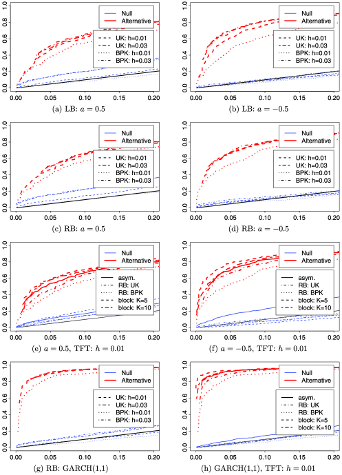
Figure 2: Change-point tests: ASP-plots for $\mathrm{AR}(1)$ process with parameter $a$ with centered exponential errors, respectively, $\mathrm{GARCH}(1,1)$, $d=\mu_{2}-\mu_{1}$, $T=200$, $\widetilde{k}=100$, BPK: Bartlett–Priestley kernel, UK: uniform kernel, LB: local bootstrap, RB: residual-based bootstrap.

In a second step, we compare the residual-based bootstrap (RB) with both kernels and bandwidth $h=0.01$ with the block permutation method of Kirch kirchblock as well as the asymptotic test. The results are given in Figure 2(e)–2(f). The TFT works best in terms of obtaining correct size, where the BPK beats the UK as already pointed out above. The power loss of the BPK is also present in comparison with the asymptotic as well as the block permutation methods; the power of the uniform kernel is also smaller than for the other method but not as severe as for the BPK. The reason probably is the sensitivity of the TFT with respect to the estimation of the underlying stationary sequence as in Corollary 3.1. In this example a mis-estimation of the change-point or the mean difference can result in an estimated sequence that largely deviates from a stationary sequence, while in the unit-root example below, this is not as important and in fact the power loss does not occur there.

The simulation results for a GARCH$(1,1)$ time series with parameters $\omega=0.3,\alpha=0.7,\beta=0.2$ [i.e., $V(t)=\sigma_{t}\varepsilon_{t}$, $\sigma_{t}^{2}=\omega+\alpha\varepsilon_{t-1}^{2}+\beta\sigma_{t-1}^{2}$, $\varepsilon_{t}\stackrel{{\scriptstyle\mathrm{i.i.d.}}}{{\sim}}N(0,1)$] are given in Figure 2(g) and 2(h), and it becomes clear that the conclusions are similar. The alternative in these plots is given by $d=0.7$.

7.2 Unit root testing

In the unit root situation we need a bootstrap sample of $V(\cdot)$ as in Corollary 3.1, where we additionally use the fact that $\{V(\cdot)\}$ has mean $0$. In this case we additionally need a bootstrap version of the mean. For simplicity we use a wild bootstrap $\mu^{*}=W(2\pi\widehat{\tau}^{2}/T)^{1/2}$, where $W$ is standard normal distributed and $\widehat{\tau}^{2}$ is as in (20), where we replace $\widehat{Z}(\cdot)$ by $\widehat{V}(\cdot)-\bar{\widehat{V}}_{T}$. The alternative in all plots is given by $\rho=0.95$.

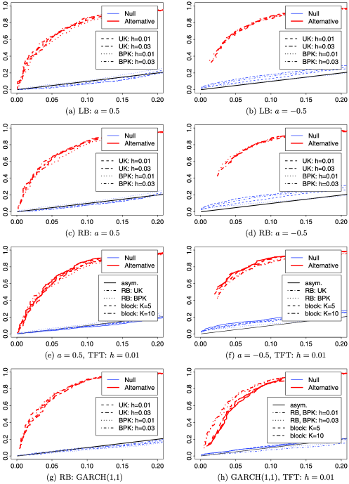
Figure 3: Unit-root tests: ASP-plots for $\mathrm{AR}(1)$ process with parameter $a$ with centered exponential errors, respectively, $\mathrm{GARCH}(1,1)$, $d=\mu_{2}-\mu_{1}$, $T=200$, $\widetilde{k}=100$, BPK: Bartlett–Priestley kernel, UK: uniform kernel, LB: local bootstrap, RB: residual-based bootstrap.

In Figure 3(a)–3(d) a comparison of different kernels and bandwidths for an $\mathrm{AR}(1)$ error sequence is given. It can be seen that again a small bandwidth yields best results, and in particular the BPK works better than the UK. Unlike in the change-point example we do not have the effect of a power loss. Furthermore unlike in change-point analysis the bootstrap works better for positively correlated errors.

A comparison with the asymptotic test as well as the block bootstrap by Paparoditis and Politis papapolitis03 can be found in Figure 3(e)–3(f). In the case of a positive correlation all methods perform approximately equivalently, at least if we use the better working Bartlett–Priestley kernel; however for a negative correlation the TFT holds the level better than the other methods.

Some results for a GARCH$(1,1)$ error sequence with parameters $\omega=0.3,\alpha=0.7,\beta=0.2$ are shown in Figure 3(g) and 3(h). In this situation a somewhat larger bandwidth of $h=0.03$ works slightly better and the TFT test leads to an improvement of the power of the tests.

It is noteworthy that the appropriate bandwidth in all cases is smaller than what one might have expected to be a good choice. A possible explanation for this is that some undersmoothing is appropriate since the back-transformation will account for some additional smoothing.

8 Conclusions

The subject of the paper is the TFT-bootstrap which is a general frequency domain bootstrap method that also generates bootstrap data in the time domain. Connections of the TFT-bootstrap with other methods including the surrogate data method of Theiler et al. theileretal92 , and the original proposals of Hurvich and Zeger hurvichzeger were thoroughly explored.

It was shown that the TFT-bootstrap samples have asymptotically the same second-order moment structure as the original time series. However, the bootstrap pseudo-series are (asymptotically) Gaussian showing that the TFT-bootstrap approximates the original time series by a Gaussian process with the same covariance structure even when the original data sequence is nonlinear; see Section 3.

Nevertheless, our simulations suggest that for small samples the TFT-bootstrap gives a better approximation to the critical values (as compared with the asymptotic ones) especially when studentizing is possible. Whether appropriate studentization results in higher-order correctness is a subject for future theoretical investigation. Choosing somewhat different types of bootstrapping in the frequency domain could also lead to higher-order correctness without bootstrapping as in, for example, Dahlhaus and Janas dahlhausjanas2 for the periodogram bootstrap.

In fact the simulations suggest that a surprisingly small bandwidth (in comparison to spectral density estimation procedures) works best. When applied in a careful manner no smoothing at all still results—in theory—in a correct second-moment behavior in the time domain (cf. Section 2.1), suggesting that due to the smoothing obtained by the back-transformation a coarser approximation in the frequency domain is necessary to avoid oversmoothing in the time domain.

9 Proofs

In this section we only give a short outline of some of the proofs. All technical details can be obtained as electronic supplementary material suppA .

We introduce the notation $a_{n}\preceq b_{n}\dvtx\Leftrightarrow a_{n}=O(b_{n})$.

The following lemma is needed to prove Lemma 3.1.

Lemma 9.1

Under Assumption $\mathcal{P}$.1, the following representation holds:

$$\frac{4\pi}{T}\sum_{k=1}^{N}f(\lambda_{k})\cos(\lambda_{k}h)=\sum_{l\in\mathbb{Z}}\gamma(h+lT)-\frac{2\pi}{T}f(0)-\frac{2\pi}{T}f(\pi)\exp(i\pi h)1_{\{T\ \mathrm{even}\}}.$$

Proof of Lemma 3.1 By Lemma A.4 in Kirch kirchfreq it holds (uniformly in $u$) that

$$\sum_{l=1}^{\lfloor mu\rfloor}\cos(\lambda_{k}l)=O\biggl{(}\min\biggl{(}\frac{T}{k},m\biggr{)}\biggr{)}.$$

Thus it holds uniformly in $u$ and $v$ that

$$\sum_{k=1}^{N}\Biggl{|}\sum_{l_{1}=1}^{\lfloor mu\rfloor}\cos(\lambda_{k}l_{1})\Biggr{|}\Biggl{|}\sum_{l_{2}=1}^{\lfloor mv\rfloor}\cos(\lambda_{k}l_{2})\Biggr{|}=O(1)\sum_{k=1}^{N}\min\biggl{(}\frac{T}{k},m\biggr{)}^{2}=O(mT).$$ (25)

By Assumptions $\mathcal{B}$.1 and $\mathcal{B}$.2 and by (2.1) it holds that

$$\operatorname{cov}^{*}\Biggl{(}\sum_{l_{1}=1}^{\lfloor mu\rfloor}Z^{*}(l_{1}),\sum_{l_{2}=1}^{\lfloor mv\rfloor}Z^{*}(l_{2})\Biggr{)}$$

$$\qquad=\frac{4\pi}{T}\sum_{l_{1}=1}^{\lfloor mu\rfloor}\sum_{l_{2}=1}^{\lfloor mv\rfloor}\sum_{k=1}^{N}f(\lambda_{k})\cos\bigl{(}\lambda_{k}(l_{1}-l_{2})\bigr{)}+o_{P}(m),$$

where the last line follows for $m/T\to 0$ as well as $m=T$ by (25). Assertion (b) follows by an application of Lemma 9.1 as well as standard representation of the spectral density as sums of auto-covariances (cf., e.g., Corollary 4.3.2 in Brockwell and Davis brockwelldavis ).

The next lemma gives the crucial step toward tightness of the partial sum process.

Lemma 9.2

Under Assumptions $\mathcal{P}$.1, $\mathcal{B}$.1–$\mathcal{B}$.3 it holds for $u<v$ and some constant $D>0$ that

$$\mathrm{E}^{*}\Biggl{(}\frac{1}{\sqrt{m}}\sum_{l=\lfloor mu\rfloor+1}^{\lfloor mv\rfloor}Z^{*}(l)\Biggr{)}^{4}\leq\bigl{(}D+o_{P}(1)\bigr{)}(v-u)^{2}.$$

Equation (25) and Lemma 9.1 yield the assertion after some standard calculations.

The next lemma gives the convergence of the finite-dimensional distribution.

Lemma 9.3

Let $S^{*}_{m}(u)=\frac{1}{\sqrt{m}}\sum_{j=1}^{\lfloor mu\rfloor}Z^{*}(j)$. [(a)]

If Assumptions $\mathcal{P}$.1, $\mathcal{B}$.1–$\mathcal{B}$.3 are fulfilled and $m/T\to 0$ we obtain for all $0<u_{1},\ldots,u_{p}\leq 1$ in probability

$$(S_{m}^{*}(u_{1}),\ldots,S_{m}^{*}(u_{p}))\stackrel{{\scriptstyle\mathcal{L}}}{{\longrightarrow}}N(0,\Sigma),$$

where $\Sigma=(c_{i,j})_{i,j=1,\ldots,p}$ with $c_{i,j}=2\pi f(0)\min(u_{i},u_{j})$.

If Assumptions $\mathcal{P}$.1, $\mathcal{B}$.1 and $\mathcal{B}$.4 are fulfilled we obtain for all $0<u_{1},\ldots,u_{p}\leq 1$ in probability

$$(S_{T}^{*}(u_{1}),\ldots,S_{T}^{*}(u_{p}))\stackrel{{\scriptstyle\mathcal{L}}}{{\longrightarrow}}N(0,\Sigma),$$

where $\Sigma=(c_{i,j})_{i,j=1,\ldots,p}$ with $c_{i,j}=2\pi f(0)(\min(u_{i},u_{j})-u_{i}u_{j})$.

For assertion (a) we use the Cramér–Wold device and prove a Lyapunov-type condition. Again arguments similar to (25) are needed. To use this kind of argument it is essential that $m/T\to 0$ because for $m=T$ the Feller condition is not fulfilled, and thus the Lindeberg condition can also not be fulfilled. Therefore a different argument is needed to obtain asymptotic normality for $m=T$. We make use of the Cramér–Wold device and Lemma 3 in Mallows mallows72 . As a result somewhat stronger assumptions are needed, but it is not clear whether they are really necessary (cf. also Remark 3.2). Proof of Theorem 3.1 Lemmas 9.2 and 9.3 ensure convergence of the finite-dimensional distribution as well as tightness, which imply by Billingsley billv2 , Theorem 13.5,

$$\Biggl{\{}\frac{1}{\sqrt{m}}\sum_{l=1}^{\lfloor mu\rfloor}\bigl{(}Z^{*}(l)-\mathrm{E}^{*}Z^{*}(l)\bigr{)}\dvtx 0\leq u\leq 1\Biggr{\}}$$

$$\qquad\stackrel{{\scriptstyle D[0,1]}}{{\longrightarrow}}\cases{\{W(u)\dvtx 0\leq u\leq 1\},&\quad$\dfrac mT\to 0$,\vspace*{2pt}\cr\{B(u)\dvtx 0\leq u\leq 1\},&\quad$m=T$.}$$

Proof of Theorem 4.1 Concerning Assumption $\mathcal{B}$.2 it holds by Assumption $\mathcal{A}$.1 that

$${\sup_{k}}|{\operatorname{var}}^{*}(x^{*}(k))-\pi f(\lambda_{k})|={\sup_{k}}|\pi\widehat{f}(\lambda_{k})-\pi f(\lambda_{k})|\stackrel{{\scriptstyle P}}{{\longrightarrow}}0.$$

Similarly we obtain Assumption $\mathcal{B}$.3 since

$$\sup_{k}\mathrm{E}^{*}(x^{*}(k))^{4}=3\pi^{2}\sup_{k}\widehat{f}(\lambda_{k})^{2}\leq 3\pi^{2}\sup_{k}f(\lambda_{k})^{2}+o_{P}(1)\leq C+o_{P}(1).$$

Concerning Assumption $\mathcal{B}$.4 let $X\stackrel{{\scriptstyle\mathcal{L}}}{{=}}N(0,1)$, then $\sqrt{\pi\widehat{f}(\lambda_{k})}X\stackrel{{\scriptstyle\mathcal{L}^{*}}}{{=}}x^{*}(k)$. Then

$$\sup_{k}d_{2}^{2}(\mathcal{L}^{*}(x^{*}(k)),N(0,\pi f(\lambda_{k}))) \leq \pi\sup_{k}\bigl{(}\sqrt{f(\lambda_{k})}-\sqrt{\widehat{f}(\lambda_{k})}\bigr{)}^{2}\mathrm{E}X^{2}$$

$$\leq {\pi\sup_{k}}{|\widehat{f}(\lambda_{k})-f(\lambda_{k})|}=o_{P}(1).$$

The proofs especially of the last statement for the residual-based as well as local bootstrap are technically more complicated but similar. Proof of Corollary 4.1 We put an index $V$, respectively, $\widehat{V}$, on our previous notation indicating whether we use $V$ or $\widehat{V}$ in the calculation of it, for example, $x_{\widehat{V}}(j)$, $x_{V}(j)$, respectively, $y_{\widehat{V}}(j)$, $y_{V}(j)$ denote the Fourier coefficients based on $\widehat{V}(\cdot)$, respectively, $V(\cdot)$.

We obtain the assertion by verifying that Assumptions $\mathcal{A}$.1, $\mathcal{A}$.2 as well as Assumption $\mathcal{A}$.4 remain true. This in turn implies Assumptions $\mathcal{B}$.2 as well as Assumption $\mathcal{B}$.3. Concerning Assumption $\mathcal{B}$.4 we show that the Mallows distance between the bootstrap r.v. based on $\widehat{V}(\cdot)$ and the bootstrap r.v. based on $V(\cdot)$ converges to 0.

The key to the proof is

$$I_{V}(j)-I_{\widehat{V}}(j)$$

$$\qquad=-\frac{1}{T}\bigl{(}F^{2}_{T}(j)+F^{2}_{T}(N+j)\bigr{)}+2\frac{1}{\sqrt{T}}x_{V}(j)F_{T}(j)$$ (26)

$$\qquad\quad{}+2\frac{1}{\sqrt{T}}y_{V}(j)F_{T}(N+j),$$

where

$$F_{T}(j):=\cases{\displaystyle\sum_{t=1}^{T}\bigl{(}V(t)-\widehat{V}(t)\bigr{)}\cos(t\lambda_{j}),&\quad$1\leq j\leq N$,\vspace*{2pt}\cr\displaystyle\sum_{t=1}^{T}\bigl{(}V(t)-\widehat{V}(t)\bigr{)}\sin(t\lambda_{j-N}),&\quad$N<j\leq 2N$.}$$

This can be seen as follows: By Theorem 4.4.1 in Kirch kirchdiss , it holds that

$$\quad\Biggl{|}\sum_{j=1}^{N}\bigl{(}\cos(t_{1}\lambda_{j})\cos(t_{2}\lambda_{j})+\sin(t_{1}\lambda_{j})\sin(t_{2}\lambda_{j})\bigr{)}\Biggr{|}\leq\cases{N,&\quad$t_{1}=t_{2}$,\cr 1,&\quad$t_{1}\neq t_{2}$.}$$ (27)

By (4.1) and an application of the Cauchy–Schwarz inequality this implies

$$|F_{T}(j)| \leq \sum_{t=1}^{T}|V(t)-\widehat{V}(t)|=o_{P}(T\alpha_{T}^{-1/2}),$$

$$\sum_{j=1}^{2N}F^{2}_{T}(j) \preceq N\sum_{t=1}^{T}\bigl{(}V(t)-\widehat{V}(t)\bigr{)}^{2}$$

$${}+\sum_{t_{1}\neq t_{2}}\bigl{|}\bigl{(}V(t_{1})-\widehat{V}(t_{1})\bigr{)}\bigl{(}V(t_{2})-\widehat{V}(t_{2})\bigr{)}\bigr{|}$$

$$= o_{P}(T^{2}\alpha_{T}^{-1}).$$

Equation (9) follows by

$$x_{V}(j)-x_{\widehat{V}}(j) = T^{-1/2}F_{T}(j),$$

$$y_{V}(j)-y_{\widehat{V}}(j) = T^{-1/2}F_{T}(N+j).$$

Proof of Lemma 5.1 Some calculations show that the lemma essentially rephrases Theorem 2.1 in Robinson robinson91 , respectively, Theorem 3.2 in Shao and Wu shaowu07 . Proof of Lemma 5.2 Some careful calculations yield

$$\sup_{1\leq l,k\leq N}|\operatorname{cov}(x(l),x(k))-\pi f(\lambda_{k})\delta_{l,k}| \to 0,$$

$$\sup_{1\leq l,k\leq N}|\operatorname{cov}(y(l),y(k))-\pi f(\lambda_{k})\delta_{l,k}| \to 0.$$

This implies by $\mathrm{E}x(k)=\mathrm{E}y(k)=0$ and an application of the Markov inequality yields

$$\frac{1}{2N}\sum_{j=1}^{N}\frac{x(j)}{\sqrt{f(\lambda_{j})}}=o_{P}(1),\qquad\frac{1}{2N}\sum_{j=1}^{N}\frac{y(j)}{\sqrt{f(\lambda_{j})}}=o_{P}(1),$$

hence assertion (a). Similar arguments using Proposition 10.3.1 in Brockwell and Davis brockwelldavis yield assertions (b) and (c). Proof of Lemma 5.3 Similar arguments as in the proof of Corollary 2.2 in Shao and Wu shaowu07 yield the result. Additionally an argument similar to Freedman and Lane freedmanlane80 is needed. Proof of Lemma 5.4 Similar arguments as in the proof of Theorem A.1 in Franke and Härdle franke yield the result. Proof of Theorem 6.1 It is sufficient to prove the assertion of Corollary 4.1 under $H_{0}$ as well as $H_{1}$, then the assertion follows from Theorem 3.1 as well as the continuous mapping theorem. By the Hájek–Renyi inequality it follows under $H_{0}$ that

$$\frac{1}{T}\sum_{t=1}^{T}\bigl{(}V(t)-\widehat{V}(t)\bigr{)}^{2} = \frac{\widehat{\widetilde{k}}}{T}(\mu-\widehat{\mu}_{1})^{2}+\frac{T-\widehat{\widetilde{k}}}{T}(\mu-\widehat{\mu}_{2})^{2}$$

$$= \frac{\log T}{T}\Biggl{(}\frac{1}{\sqrt{(\log T)\widehat{\widetilde{k}}}}\sum_{j=1}^{\widehat{\widetilde{k}}}\bigl{(}V(t)-\mathrm{E}(V(t))\bigr{)}\Biggr{)}^{2}$$

$${}+\frac{\log T}{T}\Biggl{(}\frac{1}{\sqrt{(\log T)(T-\widehat{\widetilde{k}})}}\sum_{j=\widehat{\widetilde{k}}+1}^{T}\bigl{(}V(t)-\mathrm{E}(V(t))\bigr{)}\Biggr{)}^{2}$$

$$= O_{P}\biggl{(}\frac{\log T}{T}\biggr{)},$$

which yields the assertion of Corollary 4.1. Similarly, under alternatives

$$\frac{1}{T}\sum_{t=1}^{T}\bigl{(}V(t)-\widehat{V}(t)\bigr{)}^{2}$$

$$\qquad=\frac{\min(\widehat{\widetilde{k}},\widetilde{k})}{T}(\mu_{1}-\widehat{\mu}_{1})^{2}+|d+\mu_{j}-\widehat{\mu}_{j}|^{2}\frac{|\widehat{\widetilde{k}}-{\widetilde{k}}|}{T}$$

$$\qquad\quad{}+\frac{T-\max(\widehat{\widetilde{k}},\widetilde{k})}{T}(\mu_{2}-\widehat{\mu}_{2})^{2}$$

$$\qquad=O_{P}\biggl{(}\max\biggl{(}\frac{\log T}{T},\beta_{T}\biggr{)}\biggr{)},$$

where $d=\mu_{1}-\mu_{2}$ and $j=2$ if $\widehat{\widetilde{k}}<k$ and $d=\mu_{2}-\mu_{1}$ and $j=1$ otherwise, which yields the assertion of Corollary 4.1. Proof of Theorem 6.2 Noting that $Y^{*}(k)=\sum_{j=1}^{k}V^{*}(j)$, the assertion follows from an application of Corollaries 4.1 and 3.1 as well as (22), since $V(t)-\widehat{V}(t)=(\rho-\widehat{\rho}_{T})Y(t-1)$.

Detailed proofs [doi]10.1214/10-AOS868SUPP .pdf aos868_suppl.pdf In this supplement we give the detailed technical proofs of the previous sections.

References

- (1) {barticle}[author] \bauthor\bsnmAntoch, \bfnmJ.\binitsJ., \bauthor\bsnmHušková, \bfnmM.\binitsM. and \bauthor\bsnmPrášková, \bfnmZ.\binitsZ. (\byear1997). \btitleEffect of dependence on statistics for determination of change. \bjournalJ. Statist. Plann. Inference \bvolume60 \bpages291–310. \MR1456633 \endbibitem
- (2) {bbook}[author] \bauthor\bsnmBillingsley, \bfnmP.\binitsP. (\byear1999). \btitleConvergence of Probability Measures, \bedition2nd ed. \bpublisherWiley, \baddressNew York. \MR1700749 \endbibitem
- (3) {barticle}[author] \bauthor\bsnmBraun, \bfnmW. J.\binitsW. J. and \bauthor\bsnmKulperger, \bfnmR. J.\binitsR. J. (\byear1997). \btitleProperties of a Fourier bootstrap method for time series. \bjournalComm. Statist. Theory Methods \bvolume26 \bpages1329–1336. \MR1456834 \endbibitem
- (4) {bbook}[author] \bauthor\bsnmBrillinger, \bfnmD. R.\binitsD. R. (\byear1981). \btitleTime Series. Data Analysis and Theory, \bedition2nd ed. \bpublisherHolden-Day, \baddressSan Francisco. \MR0595684 \endbibitem
- (5) {bbook}[author] \bauthor\bsnmBrockwell, \bfnmP. J.\binitsP. J. and \bauthor\bsnmDavis, \bfnmR. A.\binitsR. A. (\byear1991). \btitleTime Series: Theory and Methods, \bedition2nd ed. \bpublisherSpringer, \baddressNew York. \MR1093459 \endbibitem
- (6) {barticle}[author] \bauthor\bsnmBühlmann, \bfnmP.\binitsP. (\byear2002). \btitleBootstraps for time series. \bjournalStatist. Sci. \bvolume17 \bpages52–72. \MR1910074 \endbibitem
- (7) {barticle}[author] \bauthor\bsnmCavaliere, \bfnmG.\binitsG. and \bauthor\bsnmTaylor, \bfnmA. M. R.\binitsA. M. R. (\byear2008). \btitleBootstrap unit root tests for time series with non-stationary volatility. \bjournalEconom. Theory \bvolume24 \bpages43–71. \MR2408858 \endbibitem
- (8) {barticle}[author] \bauthor\bsnmCavaliere, \bfnmG.\binitsG. and \bauthor\bsnmTaylor, \bfnmA. M. R.\binitsA. M. R. (\byear2009). \btitleBootstrap unit root tests. \bjournalEconometric Rev. \bvolume28 \bpages393–421. \MR2555314 \endbibitem
- (9) {barticle}[author] \bauthor\bsnmCavaliere, \bfnmG.\binitsG. and \bauthor\bsnmTaylor, \bfnmA. M. R.\binitsA. M. R. (\byear2009). \btitleHeteroskedastic time series with a unit root. \bjournalEconom. Theory \bvolume25 \bpages379–400. \MR2540499 \endbibitem
- (10) {barticle}[author] \bauthor\bsnmChan, \bfnmK. S.\binitsK. S. (\byear1997). \btitleOn the validity of the method of surrogate data. \bjournalFields Inst. Commun. \bvolume11 \bpages77–97. \MR1426615 \endbibitem
- (11) {barticle}[author] \bauthor\bsnmChang, \bfnmY.\binitsY. and \bauthor\bsnmPark, \bfnmJ. Y.\binitsJ. Y. (\byear2003). \btitleA sieve bootstrap for the test of a unit root. \bjournalJ. Time Ser. Anal. \bvolume24 \bpages379–400. \MR1997120 \endbibitem
- (12) {barticle}[author] \bauthor\bsnmChiu, \bfnmS. T.\binitsS. T. (\byear1988). \btitleWeighted least squares estimators on the frequency domain for the parameters of a time series. \bjournalAnn. Statist. \bvolume16 \bpages1315–1326. \MR0959204 \endbibitem
- (13) {bbook}[author] \bauthor\bsnmCsörgő, \bfnmM.\binitsM. and \bauthor\bsnmHorváth, \bfnmL.\binitsL. (\byear1993). \btitleWeighted Approximations in Probability and Statistics. \bpublisherWiley, \baddressChichester. \MR1215046 \endbibitem
- (14) {bbook}[author] \bauthor\bsnmCsörgő, \bfnmM.\binitsM. and \bauthor\bsnmHorváth, \bfnmL.\binitsL. (\byear1997). \btitleLimit Theorems in Change-Point Analysis. \bpublisherWiley, \baddressChichester. \MR2743035 \endbibitem
- (15) {barticle}[author] \bauthor\bsnmDahlhaus, \bfnmR.\binitsR. and \bauthor\bsnmJanas, \bfnmD.\binitsD. (\byear1996). \btitleA frequency domain bootstrap for ratio statistics in time series analysis. \bjournalAnn. Statist. \bvolume24 \bpages1934–1963. \MR1421155 \endbibitem
- (16) {barticle}[author] \bauthor\bsnmDickey, \bfnmD. A.\binitsD. A. and \bauthor\bsnmFuller, \bfnmW. A.\binitsW. A. (\byear1979). \btitleDistribution of the estimators for autoregressive time series with a unit root. \bjournalJ. Amer. Statist. Assoc. \bvolume74 \bpages427–431. \MR0548036 \endbibitem
- (17) {barticle}[author] \bauthor\bsnmEfron, \bfnmB.\binitsB. (\byear1979). \btitleBootstrap methods: Another look at the jackknife. \bjournalAnn. Statist. \bvolume7 \bpages1–26. \MR0515681 \endbibitem
- (18) {barticle}[author] \bauthor\bsnmFranke, \bfnmJ.\binitsJ. and \bauthor\bsnmHärdle, \bfnmW.\binitsW. (\byear1992). \btitleOn bootstrapping kernel spectral estimates. \bjournalAnn. Statist. \bvolume20 \bpages121–145. \MR1150337 \endbibitem
- (19) {barticle}[author] \bauthor\bsnmFreedman, \bfnmD.\binitsD. and \bauthor\bsnmLane, \bfnmD.\binitsD. (\byear1980). \btitleThe empirical distribution of Fourier coefficients. \bjournalAnn. Statist. \bvolume8 \bpages1244–1251. \MR0594641 \endbibitem
- (20) {bbook}[author] \bauthor\bsnmFuller, \bfnmW. A.\binitsW. A. (\byear1996). \btitleIntroduction to Statistical Time Series, \bedition2nd ed. \bpublisherWiley, \baddressNew York. \MR1365746 \endbibitem
- (21) {barticle}[author] \bauthor\bsnmGötze, \bfnmF.\binitsF. and \bauthor\bsnmKünsch, \bfnmH. R.\binitsH. R. (\byear1996). \btitleSecond-order correctness of the blockwise bootstrap for stationary observations. \bjournalAnn. Statist. \bvolume24 \bpages1914–1933. \MR1421154 \endbibitem
- (22) {bbook}[author] \bauthor\bsnmHamilton, \bfnmJ.\binitsJ. (\byear1994). \btitleTime Series Analysis. \bpublisherPrinceton Univ. Press, \baddressPrinceton, NJ. \MR1278033 \endbibitem
- (23) {barticle}[author] \bauthor\bsnmHidalgo, \bfnmJ.\binitsJ. (\byear2003). \btitleAn alternative bootstrap to moving blocks for time series regression models. \bjournalJ. Econometrics \bvolume117 \bpages369–399. \MR2008775 \endbibitem
- (24) {barticle}[author] \bauthor\bsnmHorváth, \bfnmL.\binitsL. (\byear1997). \btitleDetection of changes in linear sequences. \bjournalAnn. Inst. Statist. Math. \bvolume49 \bpages271–283. \MR1463306 \endbibitem
- (25) {bmisc}[author] \bauthor\bsnmHurvich, \bfnmC. M.\binitsC. M. and \bauthor\bsnmZeger, \bfnmS. L.\binitsS. L. (\byear1987). \bhowpublishedFrequency domain bootstrap methods for time series. Working paper, New York Univ. \endbibitem
- (26) {barticle}[author] \bauthor\bsnmHušková, \bfnmM.\binitsM. and \bauthor\bsnmKirch, \bfnmC.\binitsC. (\byear2010). \btitleA note on studentized confidence intervals in change-point analysis. \bjournalComput. Statist. \bvolume25 \bpages269–289. \endbibitem
- (27) {binproceedings}[author] \bauthor\bsnmJanas, \bfnmD.\binitsD. and \bauthor\bsnmDahlhaus, \bfnmR.\binitsR. (\byear1994). \btitleA frequency domain bootstrap for time series. In \bbooktitleProceedings of the 26th Symposium on the Interface (\beditorJ. Sall and A. Lehman, eds.) \bpages423–425. \bpublisherInterface Foundation of North America, \baddressFairfax Station, VA. \endbibitem
- (28) {barticle}[author] \bauthor\bsnmJentsch, \bfnmC.\binitsC. and \bauthor\bsnmKreiss, \bfnmJ. P.\binitsJ. P. (\byear2010). \btitleThe multiple hybrid bootstrap—resampling multivariate linear processes. \bjournalJ. Multivariate Anal. \bvolume101 \bpages2320–2345. \endbibitem
- (29) {bmisc}[author] \bauthor\bsnmKirch, \bfnmC.\binitsC. (\byear2006). \bhowpublishedResampling methods for the change analysis of dependent data. Ph.D. thesis, Univ. Cologne. Available at http://kups.ub.uni-koeln.de/ volltexte/2006/1795/. \endbibitem
- (30) {barticle}[author] \bauthor\bsnmKirch, \bfnmC.\binitsC. (\byear2007). \btitleBlock permutation principles for the change analysis of dependent data. \bjournalJ. Statist. Plann. Inference \bvolume137 \bpages2453–2474. \MR2325449 \endbibitem
- (31) {barticle}[author] \bauthor\bsnmKirch, \bfnmC.\binitsC. (\byear2007). \btitleResampling in the frequency domain of time series to determine critical values for change-point tests. \bjournalStatist. Decisions \bvolume25 \bpages237–261. \MR2412072 \endbibitem
- (32) {bmisc}[author] \bauthor\bsnmKirch, \bfnmC.\binitsC. and \bauthor\bsnmPolitis, \bfnmD. N.\binitsD. N. (\byear2010). \bhowpublishedSupplement to “TFT-bootstrap: Resampling time series in the frequency domain to obtain replicates in the time domain.” DOI:10.1214/10-AOS868SUPP. \endbibitem
- (33) {barticle}[author] \bauthor\bsnmKokoszka, \bfnmP.\binitsP. and \bauthor\bsnmLeipus, \bfnmR.\binitsR. (\byear1998). \btitleChange-point in the mean of dependent observations. \bjournalStatist. Probab. Lett. \bvolume40 \bpages385–393. \MR1664564 \endbibitem
- (34) {barticle}[author] \bauthor\bsnmKreiss, \bfnmJ. P.\binitsJ. P. and \bauthor\bsnmPaparoditis, \bfnmE.\binitsE. (\byear2003). \btitleAutoregressive-aided periodogram bootstrap for time series. \bjournalAnn. Statist. \bvolume31 \bpages1923–1955. \MR2036395 \endbibitem
- (35) {barticle}[author] \bauthor\bsnmLahiri, \bfnmS. N.\binitsS. N. (\byear2003). \btitleA necessary and sufficient condition for asymptotic independence of discrete Fourier transforms under short- and long-range dependence. \bjournalAnn. Statist. \bvolume31 \bpages613–641. \MR1983544 \endbibitem
- (36) {bbook}[author] \bauthor\bsnmLahiri, \bfnmS. N.\binitsS. N. (\byear2003). \btitleResampling Methods for Dependent Data. \bpublisherSpringer, \baddressNew York. \MR2001447 \endbibitem
- (37) {binproceedings}[author] \bauthor\bsnmMaiwald, \bfnmT.\binitsT., \bauthor\bsnmMammen, \bfnmE.\binitsE., \bauthor\bsnmNandi, \bfnmS.\binitsS. and \bauthor\bsnmTimmer, \bfnmJ.\binitsJ. (\byear2008). \btitleSurrogate data—A qualitative and quantitative analysis. In \bbooktitleMathematical Methods in Time Series Analysis and Digital Image Processing (\beditorR. Dahlhaus, J. Kurths, P. Maas and J. Timmer, eds.). \bpublisherSpringer, \baddressBerlin. \endbibitem
- (38) {barticle}[author] \bauthor\bsnmMallows, \bfnmC. L.\binitsC. L. (\byear1972). \btitleA note on asymptotic joint normality. \bjournalAnn. Math. Statist. \bvolume43 \bpages508–515. \MR0298812 \endbibitem
- (39) {barticle}[author] \bauthor\bsnmMammen, \bfnmE.\binitsE. and \bauthor\bsnmNandi, \bfnmS.\binitsS. (\byear2008). \btitleSome theoretical properties of phase randomized multivariate surrogates. \bjournalStatistics \bvolume42 \bpages195–205. \endbibitem
- (40) {barticle}[author] \bauthor\bsnmNg, \bfnmS.\binitsS. and \bauthor\bsnmPerron, \bfnmP.\binitsP. (\byear2001). \btitleLag length selection and the construction of unit root tests with good size and power. \bjournalEconometrica \bvolume69 \bpages1519–1554. \MR1865220 \endbibitem
- (41) {binproceedings}[author] \bauthor\bsnmPaparoditis, \bfnmE.\binitsE. (\byear2002). \btitleFrequency domain bootstrap for time series. In \bbooktitleEmpirical Process Techniques for Dependent Data (\beditorH. Dehling et al., eds.) \bpages365–381. \bpublisherBirkhäuser, \baddressBoston, MA. \MR1958790 \endbibitem
- (42) {barticle}[author] \bauthor\bsnmPaparoditis, \bfnmE.\binitsE. and \bauthor\bsnmPolitis, \bfnmD. N.\binitsD. N. (\byear1999). \btitleThe local bootstrap for periodogram statistics. \bjournalJ. Time Ser. Anal. \bvolume20 \bpages193–222. \MR1701054 \endbibitem
- (43) {barticle}[author] \bauthor\bsnmPaparoditis, \bfnmE.\binitsE. and \bauthor\bsnmPolitis, \bfnmD. N.\binitsD. N. (\byear2003). \btitleResidual-based block bootstrap for unit root testing. \bjournalEconometrica \bvolume71 \bpages813–855. \MR1983228 \endbibitem
- (44) {barticle}[author] \bauthor\bsnmPaparoditis, \bfnmE.\binitsE. and \bauthor\bsnmPolitis, \bfnmD. N.\binitsD. N. (\byear2005). \btitleBootstrapping unit root tests for autoregressive time series. \bjournalJ. Amer. Statist. Assoc. \bvolume100 \bpages545–553. \MR2160558 \endbibitem
- (45) {barticle}[author] \bauthor\bsnmPark, \bfnmJ. Y.\binitsJ. Y. (\byear2003). \btitleBootstrap unit root tests. \bjournalEconometrica \bvolume71 \bpages1845–1895. \MR2015421 \endbibitem
- (46) {barticle}[author] \bauthor\bsnmPerron, \bfnmP.\binitsP. and \bauthor\bsnmNg, \bfnmS.\binitsS. (\byear1996). \btitleUseful modifications to some unit root tests with dependent errors and their local asymptotic properties. \bjournalRev. Econom. Stud. \bvolume63 \bpages435–463. \endbibitem
- (47) {barticle}[author] \bauthor\bsnmPhillips, \bfnmP. C. B.\binitsP. C. B. (\byear1987). \btitleTime series regression with a unit root. \bjournalEconometrica \bvolume55 \bpages277–301. \MR0882096 \endbibitem
- (48) {barticle}[author] \bauthor\bsnmPhillips, \bfnmP. C. B.\binitsP. C. B. and \bauthor\bsnmPerron, \bfnmP.\binitsP. (\byear1988). \btitleTesting for a unit root in time series regression. \bjournalBiometrika \bvolume75 \bpages335–346. \MR0946054 \endbibitem
- (49) {barticle}[author] \bauthor\bsnmPolitis, \bfnmD. N.\binitsD. N. (\byear2003). \btitleAdaptive bandwidth choice. \bjournalJ. Nonparametr. Stat. \bvolume15 \bpages517–533. \MR2017485 \endbibitem
- (50) {barticle}[author] \bauthor\bsnmPolitis, \bfnmD. N.\binitsD. N. (\byear2003). \btitleThe impact of bootstrap methods on time series analysis. \bjournalStatist. Sci. \bvolume18 \bpages219–230. \MR2026081 \endbibitem
- (51) {bmisc}[author] \bauthor\bsnmPolitis, \bfnmD. N.\binitsD. N. (\byear2009). \bhowpublishedHigher-order accurate, positive semi-definite estimation of large-sample covariance and spectral density matrices. Preprint. Paper 2005-03R, Dept. Economics, UCSD. Available at http://repositories.cdlib.org/ ucsdecon/2005-03R. \endbibitem
- (52) {bbook}[author] \bauthor\bsnmPriestley, \bfnmM. B.\binitsM. B. (\byear1981). \btitleSpectral Analysis and Time Series. \bpublisherAcademic Press, \baddressLondon. \endbibitem
- (53) {barticle}[author] \bauthor\bsnmRobinson, \bfnmP. M.\binitsP. M. (\byear1991). \btitleAutomatic frequency domain inference on semiparametric and nonparametric models. \bjournalEconometrica \bvolume59 \bpages1329–1363. \MR1133037 \endbibitem
- (54) {barticle}[author] \bauthor\bsnmRomano, \bfnmJ. P.\binitsJ. P. and \bauthor\bsnmThombs, \bfnmL. A.\binitsL. A. (\byear1996). \btitleInference for autocorrelations under weak assumptions. \bjournalJ. Amer. Statist. Assoc. \bvolume91 \bpages590–600. \MR1395728 \endbibitem
- (55) {barticle}[author] \bauthor\bsnmShao, \bfnmX.\binitsX. and \bauthor\bsnmWu, \bfnmW. B.\binitsW. B. (\byear2007). \btitleAsymptotic spectral theory for nonlinear time series. \bjournalAnn. Statist. \bvolume35 \bpages1773–1801. \MR2351105 \endbibitem
- (56) {bincollection}[author] \bauthor\bsnmStock, \bfnmJ. H.\binitsJ. H. (\byear1999). \btitleA class of tests for integration and cointegration. In \bbooktitleCointegration, Causality, and Forecasting—Festschrift in Honour of Clive W. J. Granger (\beditorR. F. Engle and H. White, eds.) \bpages137–167. \bpublisherOxford Univ. Press, \baddressNew York. \endbibitem
- (57) {barticle}[author] \bauthor\bsnmTheiler, \bfnmJ.\binitsJ., \bauthor\bsnmEubank, \bfnmS.\binitsS., \bauthor\bsnmLongtin, \bfnmA.\binitsA., \bauthor\bsnmGaldrikan, \bfnmB.\binitsB. and \bauthor\bsnmFarmer, \bfnmJ. D.\binitsJ. D. (\byear1992). \btitleTesting for nonlinearity in time series: The method of surrogate data. \bjournalPhys. D \bvolume58 \bpages77–94. \endbibitem
- (58) {bmisc}[author] \bauthor\bsnmWu, \bfnmW. B.\binitsW. B. (\byear2008). \bhowpublishedPersonal communication. \endbibitem