Parameterized Uniform Complexity in Numerics:
from Smooth to Analytic, from $\mathcal{NP}$–hard to Polytime

Abstract

The synthesis of classical Computational Complexity Theory with Recursive Analysis provides a quantitative foundation to reliable numerics. Here the operators of maximization, integration, and solving ordinary differential equations are known to map (even high-order differentiable) polynomial-time computable functions to instances which are ‘hard’ for classical complexity classes $\mathcal{NP}$, $\#\mathcal{P}$, and $\mathcal{CH}$; but, restricted to analytic functions, map polynomial-time computable ones to polynomial-time computable ones — non-uniformly!

We investigate the uniform parameterized complexity of the above operators in the setting of Weihrauch’s TTE and its second-order extension due to Kawamura&Cook (2010). That is, we explore which (both continuous and discrete, first and second order) information and parameters on some given $f$ is sufficient to obtain similar data on $\operatorname{Max}f$ and $\int f$; and within what running time, in terms of these parameters and the guaranteed output precision $2^{-n}$.

It turns out that Gevrey’s hierarchy of functions climbing from analytic to smooth corresponds to the computational complexity of maximization growing from polytime to $\mathcal{NP}$-hard. Proof techniques involve mainly the Theory of (discrete) Computation, Hard Analysis, and Information-Based Complexity.

1 Motivation and Introduction

Numerical methods provide practical solutions to many, and particularly to very large, problems arising for instance in Engineering. Nonlinear partial differential equations for instance are usually treated by discretizing the domain of the solution function space, i.e. approximating the latter by a high but finite dimensional space. Due to the nonlinearity, sub-problems may involve (low-dimensional) numerical integration and maximization and are regularly handled by standard methods. For instance Newton Iterations locally converge quadratically to a root $x_{0}$ of $f^{\prime}$, that is, a candidate optimum.

We thus record that numerical science has devised a variety of impressive methods working in practice very well — in terms of an intuitive conception of efficiency. A notion capturing this formally, on the other hand, is at the core of the Theory of Computation and has led to standard complexity classes like $\mathcal{P}$, $\mathcal{NP}$, $\mathcal{UP}$, $\#\mathcal{P}$, $\mathcal{CH}$, and $\mathcal{PSPACE}$: for discrete problems, that is, over sequences of bits encoding, say, integers or graphs [Papa94]. To quote from [BCSS98, §1.4]:

The developments described in the previous section (and the next) have given a firm foundation to computer science as a subject in its own right. Use of the Turing machines yields a unifying concept of the algorithm well formalized. […] The situation in numerical analysis is quite the opposite. Algorithms are primarily a means to solve practical problems. There is not even a formal definition of algorithm in the subject. […] Thus we view numerical analysis as an eclectic subject with weak foundations; this certainly in no way denies its great achievements through the centuries.

Recursive Analysis is the theory of computation over real numbers by rational approximations up to prescribable absolute error $2^{-n}$. Initiated by Alan Turing (in the very same work that introduced the machine now named after him [Turi37]) it provides a computer scientific foundation to reliable numerics [AFL96] and computer-assisted proofs [Rump04] in unbounded precision; cmp., e.g., [KLRK98, BLWW04, BrCo06].

Remark 1.1

Mainstream numerics is usually scrupulous about constant factor gains or losses (e.g. $5\times$) in running time. This generally means an implicit restriction to hardware supported calculations, that is, to double and in particular to fixed-precision arithmetic.

1. Alternative approaches that, in order to approximate the result with double accuracy, use unbounded precision for intermediate calculations, therefore reside in a ‘blind spot’ — which Recursive Analysis may shed some light on [MüKo10].

2. Inputs $x$ are in classical numerics generally considered ‘exact’; equivalently: both subtraction and the Heaviside function regarded as computable.

3. Outputs $y$, on the other hand, constitute mere approximations to the ‘true’ values $f(x)$. In consequence, this notion of real computation necessarily lacks closure under composition [Yap04, p.325].

The latter is more than just a conceptual annoyance: the (approximate) result of one subroutine cannot in general be fed as argument to another in order to obtain a (provably always) correct algorithm, thus spoiling the modular approach to software development!

Rooted in the Theory of Computation, Recursive Analysis on the other hand is closed under composition — and interested only in asymptotic algorithmic behaviour, that is, ignoring constant factors in running times.

Remark 1.2

Libraries based on this model of computation [Müll01, Lamb07], on calculations that suffice with double precision (and thus do not actually make use of the enhanced power) can generally be expected to run 20 to 200 times slower than a direct implementation. Even in this limited realm they are useful for fast numerical prototyping, that is, for a first quick-and-dirty coding of some new algorithmic approach to empirically explore its typical running time behaviour and stability properties. Indeed,

1. accuracy issues are taken care of by the machine automatically

2. closure under composition allows for modularly combining subroutines

3. chosen from, or contributing to, a variety of standard real functions and non-/linear operators.

Their full power of course lies in computations involving intermediate or final results with unbounded guaranteed precision [Ret08b].

Recursive Analysis has over the last few decades evolved into a rich and flourishing theory with many classical results in real and complex analysis investigated for their computability. That includes, in addition to numbers, also ‘higher-type’ objects such as (continuous) functions, (closed and open) subsets, and operators thereon [Zieg04, Schr07]: by fixing some suitable encoding of the arguments (real numbers, continuous functions, closed/open subsets) into infinite binary strings. More precisely the Type-2 Theory of Effectivity (TTE, cmp. Remark 1.8 below) studies and compares such encodings (so-called representations) [Weih00]: mostly qualitatively in the sense of which mappings they render computable and which not.

Fact 1.3

Concerning complexity theory, Ker-I Ko and Harvey Friedman have constructed in [KoFr82] certain smooth (i.e. $C^{\infty}$) functions $f,g:[0;1]\to[0;1]$ computable in time polynomial in the output precision $n$ (short: polytime) and proved the following:

1. The function $\operatorname{Max}(f):=\big{(}[0;1]\ni t\mapsto\max\{f(x):0\leq x\leq t\}\big{)}\in C^{\infty}[0;1]$ is again polytime iff $\mathcal{P}=\mathcal{NP}$ holds; cmp. [Ko91, Theorem 3.7].

2. The function $\int g:=\big{(}[0;1]\ni t\mapsto\int_{0}^{t}g(x)\,dx\big{)}\in C^{\infty}[0;1]$ is polytime for every polytime $f\in C[0;1]$  iff  $\mathcal{P}=\#\mathcal{P}$; cmp. [Ko91, Theorem 5.33].

3. More recently, one of us succeeded in constructing a polytime Lipschitz–continuous function $h:[0;1]\times[-1;1]\to[-1;1]$ such that the unique solution $u:=\operatorname{dsolve}(h):[0;1]\to[-1;1]$ to the ordinary differential equation

   $$u^{\prime}(t)\;=\;h\big{(}t,u(t)\big{)},\quad u(0)=0$$ (1)

   is again polytime iff $\mathcal{P}=\mathcal{PSPACE}$ [Kawa10].

4. Restricted to polytime right-hand sides $h\in C^{k}$, $\operatorname{dsolve}(h)$ is again polytime iff $\mathcal{P}=\mathcal{CH}$ [KORZ12].

Put differently: If numerical methods could indeed calculate maxima (or even integrals or solve ODEs) efficiently with prescribable error in the worst case, this would mean a positive answer to the first Millennium Prize Problem (and beyond); cmp. [Smal98]! The proof of Fact 1.3a) will be recalled in Example 1.14 below.

Remark 1.4

1. We consider here the real problems as operators $\mathbb{O}$ mapping functions $f$ to functions $\mathbb{O}(f)$, that is, depending on the upper end $t$ of the interval $[0;t]$ which the given $f$ is to be maximized, integrated, or the ODE solved on. Fixing $t:=1$ amounts to functionals $f\mapsto\Lambda(f):=\mathbb{O}\big{(}f\big{)}(1)$; and the worst-case complexity of the single real numbers $\|f\|=\operatorname{Max}\big{(}f\big{)}(1)$ and $\int_{0}^{1}f(x)\,dx$ for polytime $f\in C^{\infty}[0;1]$ corresponds to famous open questions concerning unary complexity classes $\mathcal{P}_{1}$, $\mathcal{NP}_{1}$, and $\#\mathcal{P}_{1}$ [Ko91, Theorems 3.16+5.32]; recall Mahaney’s Theorem.

2. It has been conjectured [Shar12] that the difficulty of optimizing some (smooth) function $f:[0;1]\to[0;1]$ may arise from it having many maxima; and indeed this is the case for the ‘bad’ function $f$ according to Fact 1.3a). However a modification of the construction proving [Ko91, Theorem 3.16] yields a polytime computable smooth $\tilde{f}$ such that, for every $x\in[0;1]$, $\tilde{f}\big{|}_{[0;x]}$ attains its maximum in precisely one point while relating the complexity of the single real $\operatorname{Max}\big{(}\tilde{f}\big{)}(1)$ to the complexity class $\mathcal{UP}_{1}$ of unary decision problems accepted by a nondeterministic polytime Turing machine with at most one accepting computation for each input. Recall the Valiant–Vazirani Theorem and that the open question “$\mathcal{P}\neq\mathcal{UP}$” is equivalent to that of the existence of cryptographic one-way functions [Papa94, Theorem 12.1].

Indeed, the numerics community seems little aware of these connections. And, as a matter of fact, such ignorance may almost have some justification: The above functions $f$ and $g$ and $h$, although satisfying strong regularity conditions, are ‘artificial’ in any intuitive sense and clearly do not arise in practical applications. This, on the other hand, raises

Question 1.5

1. Which functions are the ones numerical practitioners regularly and implicitly allude to when claiming to be able to efficiently calculate their maximum, integral, and ODE solution?

2. More formally, on which (classes $\mathcal{F}_{k}$ of) functions do these operations become computable in polynomial time $\mathcal{O}(n^{d})$ for some (and, more precisely, for which) $d=d(k)\in\mathbb{N}$?

We admit that numerics as pursued in Engineering might not really need to answer this question but be happy as long as, say, MatLab readily solves those particular instances encountered everyday. Such a pragmatic approach seems indeed compatible for instance with the spirit of the NAG library:

nag_opt_one_var_deriv(e04bbc) normally computes a sequence of $x$ values which tend in the limit to a minimum of $F(x)$ subject to the given bounds.

Both Mathematics and (theoretical) Computer Science, however, do come with a tradition of explicitly stating prerequisitesf:Schwarz to theorems and specifying the domains and running-time bounds to (provably correct) algorithms, respectively: crucial for modularly combining known results/algorithms to obtain new ones; recall the end of Remark 1.1. In the case of real computation, finding such a specification for maximization and integration, say, amounts to answering Question 1.5b). Moreover, the answer cannot include all polytime $C^{k}$–functions for any $k\in\mathbb{N}$ according to Fact 1.3. On the other hand, we record

Example 1.6

One important (but clearly too small) class $\mathcal{F}$ of functions $f:[-1;1]\to\mathbb{R}$, for which $\operatorname{Max}f$, $\int f$, and $\operatorname{dsolve}(f)$ as well as derivatives $f^{(j)}$ are known polytime whenever $f$ is, consists of the real analytic ones: those locally admitting power series expansions, cmp. [Ko91, p.208] and see [Müll87, MüMo93, Müll95, BGP11]; equivalently [KrPa02, Proposition 1.2.12]: those satisfying, for some $A,K\in\mathbb{N}$,

$$\forall|x|\leq 1,\quad\forall j\in\mathbb{N}:\qquad|f^{(j)}(x)|\;\leq\;A\cdot K^{j}\cdot j!\enspace.$$ (2)

Indeed, the following is the standard example of a smooth but non-analytic function:

$$h\;:[-1;1]\;\ni\;x\;\mapsto\;\left\{\begin{array}[]{ll}\exp(-1/x)&x>0\\ 0&x\leq 0\end{array}\right.$$

Based on l’Hôspital’s rule it is easy to verify that $h$ is continuous at $x_{0}=0$ and differentiable arbitrarily often with $h^{(j)}(0)=0$, hence having Taylor expansion around $x_{0}$ disagree with $h$.

Note that both Fact 1.3 and Example 1.6 are stated non-uniformly in the sense of ignoring how $f$ is algorithmically transformed into, say, $\operatorname{Max}f$. Consisting of lower complexity bounds, this makes Fact 1.3 particularly strong; whereas as upper bounds Example 1.6 merely asserts, whenever there exists some $d\in\mathbb{N}$ and an algorithm $\mathcal{A}$ approximating $f$ within time $\mathcal{O}(m^{d})$ up to error $2^{-m}$, the existence of some $e\in\mathbb{N}$ and an algorithm $\mathcal{B}$ approximating $\operatorname{Max}f$ up to error $2^{-n}$ within time $\mathcal{O}(n^{e})$: both the dependence of $\mathcal{B}$ on $\mathcal{A}$ and that of $e$ on $d$ are ignored. Put differently, the proofs of Example 1.6 may and do implicitly make use of many integer parameters of $f$ (such as numerator and denominator of starting points for Newton’s Iteration converging to a root $x_{0}$ of $f^{\prime}$ of known multiplicity where $f$ attains its maximum) since, nonuniformly, they constitute simply constants. Useful uniform (computability and) upper complexity bounds like in [BGP11], on the other hand, fully specify

1. which information on $f$ is employed as input

2. which asymptotic running times are met in the worst case

3. in terms of which parameters (in addition to the output precision $n$).

The present work extends the Type-2 Theory of Effectivity and Complexity [Weih03] to such parameterized, uniform claims. We focus here on operators and upper complexity bounds, that is, fully specified provably correct algorithms.

Let us illustrate the relevance of integer parameters, and its difference from integral advice [Zieg12], to real computation of (multivalued) functions:

Example 1.7

1. On the entire real line, the exponential function and binary addition and multiplication are computable — but not within time bounded in terms of the output precision $n$ only: Because already the integral part of the argument $x$ requires time reading and printing depending on (any integer upper bound $k$ on) $x\to\pm\infty$.

2. Restricted to real intervals $[-k;k]$, on the other hand, $\exp:|_{[-k;k]}$ is computable in time polynomial in $\mathcal{O}(n+k)$, noting that $\lfloor\exp(k)\rfloor$ has binary length of order $k\cdot\log k$.
   Similarly, binary addition and multiplication on $[-k;k]\times[-k;k]$ are computable in time polynomial in $\mathcal{O}(n+\log k)$.
   Here and in the sequel, abbreviate $\log(k):=\lceil\log_{2}(k+1)\rceil$.

3. Given a real symmetric $d\times d$–matrix $A$, finding (in a multivalued way) some eigenvector is uncomputable.

4. However when given, in addition to $A$, also the integer $\ell(A):=\min_{\lambda\in\sigma(A)}\lfloor\log_{2}\dim\operatorname{kernel}(A-\lambda\operatorname{id})\rfloor\in\{0,\ldots,\lfloor 1+\log_{2}d\rfloor\}$, some eigenvector can be found computably and,

5. given the integer $L(A):=\operatorname{Card}\sigma(A)\in\{1,\ldots,d\}$, even an entire basis of eigenvectors, i.e. the matrix can be diagonalized computably.

The rest of this section recalls the state of the art on real complexity theory with its central notions and definitions.

1.1 Computability and Complexity Theory of Real Numbers and Sequences

A real number $x$ is considered computable (that is an element of $\mathbb{R}_{\text{c}}$) if any (equivalently: all) of the following conditions hold [Weih00, §4.1+Lemma 4.2.1]:

a1)

The (or any) binary expansion $b_{n}\in\{0,1\}$ of $x=\sum_{n\geq-N}b_{n}2^{-n}$ is recursive.

a2)

A Turing machine can produce dyadic approximations to $x$ up to prescribable error $2^{-n}$, that is, compute an integer sequence $a:\mathbb{N}\ni n\mapsto a_{n}\in\mathbb{Z}$ (output encoded in binary) with $|x-a_{n}/2^{n+1}|\leq 2^{-n}$; cmp. e.g. [Eige08, Definition 3.35].

a3)

A Turing machine can output rational sequences $(c_{n})$ and $(\epsilon_{n})$ with $|x-c_{n}|\leq\epsilon_{n}\to 0$; cmp. e.g. [PERi89, Definition 0.3].

a4)

$x$ admits a recursive signed digit expansion, that is a sequence $s_{n}\in\{\textup{{0}},-\textup{{1}},+\textup{{1}}\}$ with $x=\sum_{n=-N}s_{n}2^{-n}$.

Moreover the above conditions are strictly stronger than the following

a5)

A Turing machine can output rational sequences $(c^{\prime}_{n})$ with $c^{\prime}_{n}\to x$.

In fact relaxing to (a5) is equivalent to permitting oracle access to the Halting problem [Ho99]! We also record that the equivalence among (a2) to (a4), but not to (a1), holds even uniformly.

Remark 1.8

TTE constitutes a convenient framework for naturally inducing, combining, and comparing encodings of general continuous universes $X$ like $\mathbb{R}$:

1. Formally, a representation $\xi$ of $X$ is a surjective partial mapping from Cantor space $\{\textup{{0}},\textup{{1}}\}^{\omega}$ to $X$ [Weih00, §3].

2. And $\xi$–computing some $x$ means to output a $\xi$–name (out of possibly many) of $x$, that is, print onto some non-rewritable [Zieg07] tape an infinite binary sequence $\bar{\sigma}=(\sigma_{n})_{{}_{n}}\in\{\textup{{0}},\textup{{1}}\}^{\omega}$ with $\xi(\bar{\sigma})=x$.

3. Representations $\xi$ of $X$ and $\upsilon$ of $Y$ canonically give rise to one, called $\xi\times\upsilon$, of $X\times Y$: A $\xi\times\upsilon$–name of $(x,y)$ is an infinite binary sequence $(\sigma_{0},\tau_{0},\sigma_{1},\tau_{1},\ldots)$ where $\bar{\sigma}$ constitutes a $\xi$–name of $x$ and $\bar{\tau}$ an $\upsilon$–name of $y$.

4. Similarly, a countable family of representations $\xi_{j}$ of $X_{j}$ canonically induces the representation $\prod_{j}\xi_{j}$ of $\prod_{j}X_{j}$ as follows: For a fixed computable bijection $\langle\,\cdot\,,\,\cdot\,\rangle:\mathbb{N}\times\mathbb{N}\to\mathbb{N}$, $\bar{\sigma}=(\sigma_{k})_{{}_{k}}$ is a $\prod_{j}\xi_{j}$–name of $\prod_{j}x_{j}$ iff $(\sigma_{\langle n,j\rangle})_{{}_{n}}$ is a $\xi_{j}$–name of $x_{j}$ for every $j$.

5. The representation $\operatorname{binary}$ of $\mathbb{N}$ encodes integers in binary self-delimited with trailing zeros: $\operatorname{binary}(\textup{{1}}\,b_{0}\,\textup{{1}}\,b_{1}\,\cdots\,\textup{{1}}\,b_{n}\,\textup{{0}}^{\omega}):=\sum_{j=0}^{n}b_{j}2^{j}$.
   Representation $\operatorname{unary}$ of $\mathbb{N}$ encodes integers in unary: $\operatorname{unary}(\textup{{1}}^{n}\,\textup{{0}}^{\omega}):=n$.

6. Note that the bijection $\operatorname{bin}:\{\textup{{0}},\textup{{1}}\}^{*}\to\mathbb{Z}$ with

   $$(\textup{{1}}\,w_{n-1}\cdots w_{1}w_{0}) \mapsto \phantom{1-(}w_{0}+2w_{1}+\cdots+2^{n-1}w_{n-1}+2^{n},$$

   $$(\textup{{0}}\,w_{n-1}\cdots w_{1}w_{0}) \mapsto 1-(w_{0}+2w_{1}+\cdots+2^{n-1}w_{n-1}+2^{n})$$

   itself is technically not a representation – but useful as a building block. By abuse of name we denote its inverse also by $\operatorname{bin}$.

Concerning real numbers, the equivalences between (a1) to (a4) refer to computability. Not too surprisingly, they break up under the finer perspective of complexity; some notions even become useless [Weih00, Example 7.2.1]. On the other hand, (a2) and (a4) do lead to uniformly quadratic-time equivalent notions [Weih00, Example 7.2.14]. Somehow arbitrarily, but in agreement with iRRAM’s internal data representation, we focus on the following formalization in TTE:

Definition 1.9

1. Call $x\in\mathbb{R}$ computable in time $t(n)$ if a Turing machine can, given $n\in\mathbb{N}$, produce within $t(n)$ steps $\vec{w}\in\{\textup{{0}},\textup{{1}}\}^{*}$ with $|x-\operatorname{bin}(\vec{w})/2^{n+1}|\leq 2^{-n}$.

2. A $\rho_{\text{\rm dy}}$–name of $x\in\mathbb{R}$ is (an infinite sequence of 0’s and 1’s encoding similarly to Remark 1.8f) a sequence $a_{n}\in\mathbb{Z}$ such that $|x-a_{n}/2^{n+1}|\leq 2^{-n}$ holds.

3. A $\rho_{\text{\rm dy}}^{2}$–name of $z\in\mathbb{C}$ consists of a $\rho_{\text{\rm dy}}$–name according to b) of $\operatorname{Re}(z)$ and one of $\operatorname{Im}(z)$, both infinite sequences interleaved into a single (Remark 1.8c).

4. A sequence $(x_{j})\subseteq\mathbb{R}$ is computable in time $t(n,j)$ if a Turing machine can, given $n,j\in\mathbb{N}$, produce within $t(n,j)$ steps some $a\in\mathbb{Z}$ (in binary) with $|x_{j}-a/2^{n+1}|\leq 2^{-n}$.

5. A $\rho_{\text{\rm dy}}^{\omega}$–name of a real sequence $(x_{j})$ is a sequence $(a_{j})\in\mathbb{Z}$, encoded into an infinite binary string as above, such that $|x_{j}-a_{\langle n,j\rangle}|\leq 2^{-n}$.

6. Here and in the sequel fix the Cantor pairing function $\langle n,j\rangle=n+(n+j)\cdot(n+j+1)/2$.

Note that the running time bound in a) is expressed in terms of the output precision $n$; which corresponds to classical complexity theory based on input length by having the argument $n$ encoded in unary. Indeed, the output $a\in\mathbb{Z}$ will have length $\Theta(n+\log|x|)$ in Landau notation. Within a $\rho_{\text{\rm dy}}$–name of $x$ according to b), the $\mathcal{O}(\log|x|+n)$ digits of $a_{n}$ similarly start roughly at position $n\cdot(n+\log|x|)$. Similarly, since $\langle m,j\rangle\leq\mathcal{O}(m^{2}+j^{2})$, the digits of $a_{\langle m,j\rangle}$ start within a $\rho_{\text{\rm dy}}^{\omega}$–name of $(x_{j})$ at position $n\approx(m^{2}+j^{2})\cdot(m+\max_{i\leq j}\log|x_{i}|)$. We also record that both the mapping $(m,j)\mapsto\langle m,j\rangle$ and its inverse are classically quadratic-time computable.

1.2 Type-2 Computability and Complexity Theory: Functions

Concerning a real function $f:[0;1]\to\mathbb{R}$, the following conditions are well-known equivalent and thus a reasonable notion of computability [Grze57], [PERi89, §0.7], [Weih00, §6.1], [Ko91, §2.3], [LLM01, Définition 2.1.1].

b1)

A Turing machine can output a sequence of (degrees and lists of coefficients of) univariate dyadic polynomials $P_{n}\in\mathbb{D}[X]$ such that $\forall n\in\mathbb{N}:\|f-P_{n}\|\leq 2^{-n}$ holds, where $\mathbb{D}:=\bigcup_{n}\mathbb{D}_{n}$ and $\|f\|:=\max\{|f(x)|:0\leq x\leq 1\}$.

b2)

A Turing machine can, upon input of every $\rho_{\text{\rm dy}}$–name of some $x\in[0;1]$, output a $\rho_{\text{\rm dy}}$–name of $f(x)$.

b3)

There exists an oracle Turing machine $\mathcal{M}^{?}$ which, upon input of each $n\in\mathbb{N}$ and for every (discrete function) oracle answering queries “$m\in\mathbb{N}$” with some $a\in\mathbb{D}_{m+1}$ such that $|x-a|\leq 2^{-m}$, prints some $b\in\mathbb{D}_{n+1}$ with $|f(x)-b|\leq 2^{-n}$.

In particular every (even relatively, i.e. oracle) computable $f:[0;1]\to\mathbb{R}$ is necessarily continuous. This gives rise to two causes for noncomputability: a (classical) recursion theoretic and a topological one; cmp. Figure 1b). More precisely, every $f\in C[0;1]$ is computable relative so some appropriate oracle; cmp. [Weih00, Theorem 3.2.11].

Remark 1.10

1. The above (equivalent) notions of computability are uniform in the sense that $x$ is considered given as argument from which the value $f(x)$ has to be produced. The nonuniform relaxation asks of whether, for every $x\in[0;1]\cap\mathbb{R}_{\text{c}}$, $f(x)$ is again computable: possibly requiring separate algorithms to do so for each of the (countably many) $x\in[0;1]\cap\mathbb{R}_{\text{c}}$. For instance the totally discontinuous Dirichlet function is trivially computable in this (thus too weak) sense.

2. Defining computable functions also on non-computable arguments (as above) is known to avoid certain pathologies in the partial case [Weih00, Example 9.6.5] while making no difference on well-behaved domains [Weih00, Theorem 9.6.6].

3. For spaces $X,Y$ with respective representations $\xi,\upsilon$, TTE defines a $(\xi,\upsilon)$–realizer of a (possibly partial and/or multivalued) function $f:\subseteq X\rightrightarrows Y$ to be a partial mapping $F:\subseteq\{\textup{{0}},\textup{{1}}\}^{\omega}\to\{\textup{{0}},\textup{{1}}\}^{\omega}$ such that, for every $\xi$–name $\bar{\sigma}$ of every $x\in\operatorname{dom}(f)$, $\tau:=F(\bar{\sigma})$ is a $\upsilon$–name of some $y\in f(x)$. And $f$ is called $(\xi,\upsilon)$–computable if it admits a computable $(\xi,\upsilon)$–realizer. Notion (b2) thus amounts to $(\rho_{\text{\rm dy}},\rho_{\text{\rm dy}})$–computability.

Concerning complexity, (b2) and (b3) have turned out as polytime equivalent but different from (b1); cf. [Ko91, §8.1] and [Weih00, Theorem 9.4.3]. So as opposed to discrete complexity theory, running time is not measured in terms of the input length (which is infinite anyway) but in terms of the output precision parameter $n$ in (b3); and for (b2) in terms of the time until the $n$-th digit of the infinite binary output string appears: in both cases uniformly in (i.e. w.r.t. the worst-case over all) $x\in[0;1]$. Indeed the dependence on $x$ can be removed by taking the maximum running time over $[0;1]$, a compact set [Weih00, Theorem 7.2.7]. On non-compact domains, on the other hand, the running time will in general admit no bound depending on the output precision $n$ only; recall Example 1.7a) and see [Weih00, Exercise 7.2.10].

The qualitative topological condition of continuity is a prerequisite to computability of a function. Its quantitative refinement capturing sensitivity on the other hand corresponds to a lower bound on the complexity [Ko91, Theorem 2.19]:

Fact 1.11

If $f:[0;1]\to\mathbb{R}$ is computable in the sense of (b3) within time $t(n)$, then the function $\mu:\mathbb{N}\ni n\mapsto t(n+2)\in\mathbb{N}$ constitutes a modulus of continuity to $f$ in the sense that the following holds:

$$\forall x,y\in\operatorname{dom}(f):\quad|x-y|\leq 2^{-\mu(n)}\;\Rightarrow\;|f(x)-f(y)|\leq 2^{-n}\enspace.$$ (3)

In particular every polytime computable function necessarily has a polynomial modulus of continuity; and, conversely, each $f:[0;1]\to\mathbb{R}$ satisfying Equation (3) for polynomial $\mu$ is polytime computable relative to some oracle.

The Time Hierarchy Theorem in classical complexity theory constructs a set $E\subseteq\mathbb{N}$ decidable in exponential but not in polynomial time. Appropriately encoded, this in turn yields a real number $y[E]$ of similar complexity [Weih00, Lemma 7.2.9]; and the same holds for the constant function $[0;1]\ni x\mapsto y[E]$ [Weih00, Corollary 7.2.10]: computable within exponential but not in polynomial time. We remark that, again and as opposed to this recursion theoretic construction, also quantitative topological reasons lead to an (even explicitly given) function with such properties; cmp. Figure 1b):

Example 1.12

The following function is computable in exponential time, but not in polynomial time — and oracles do not help:

$$f:(0;1]\;\ni\;x\;\mapsto\;1/\ln(e/x)\;\in\;(0;1],\qquad f(0)=0\enspace.$$

Proof

Note that monotone $f$ is obviously computable on $(0;1]$, and continuous in 0; in fact effectively continuous but with exponential modulus of continuity. More precisely, $f(2^{-m})=1/(1+m\cdot\ln 2)\overset{!}{\leq}2^{-n}\Leftrightarrow m\geq(2^{n}-1)/\ln 2$. Therefore arguments $x=2^{-m}$ must be known from zero (i.e. and with precision at least $m$ exponential in $n$) in order to assert the value $f(x)$ different from $f(0)=0$ up to error $2^{-n}$. ∎

	recursion theoretic	topological
non-computable	$f(x)\equiv y[H]$	$f(x)=\operatorname{sgn}(x)$
exponential complexity	$f(x)\equiv y[E]$	$f(x)=1/\ln(e/x)$

Figure 1: a) The graph of $f(x)=1/\ln(e/x)$ from Example 1.12 demonstrating its exponential rise from 0.
b) Lower bound techniques in real function computation; $H\subseteq\mathbb{N}$ is the Halting problem and $\mathbb{N}\supseteq E\in\text{\sf EXP}\setminus\mathcal{P}$.

Concerning computational complexity on spaces other than $\mathbb{R}$, consider

Definition 1.13

1. A partial function $F:\subseteq\{\textup{{0}},\textup{{1}}\}^{\omega}\to\{\textup{{0}},\textup{{1}}\}^{\omega}$ is computable in time $t:\mathbb{N}\to\mathbb{N}$ if a Type-2 Machine can, given $\bar{\sigma}\in\operatorname{dom}(F)$, produce $\bar{\tau}=F(\bar{\sigma})$ such that the $n$-th symbol of $\bar{\tau}$ appears within $t(n)$ steps.

2. For representations $\xi$ of $X$ and $\upsilon$ of $Y$, a (possibly partial and multivalued) function $f:\subseteq X\rightrightarrows Y$ is computable in time $t:\mathbb{N}\to\mathbb{N}$ if it has a $(\xi,\upsilon)$–realizer $F$ according to a).

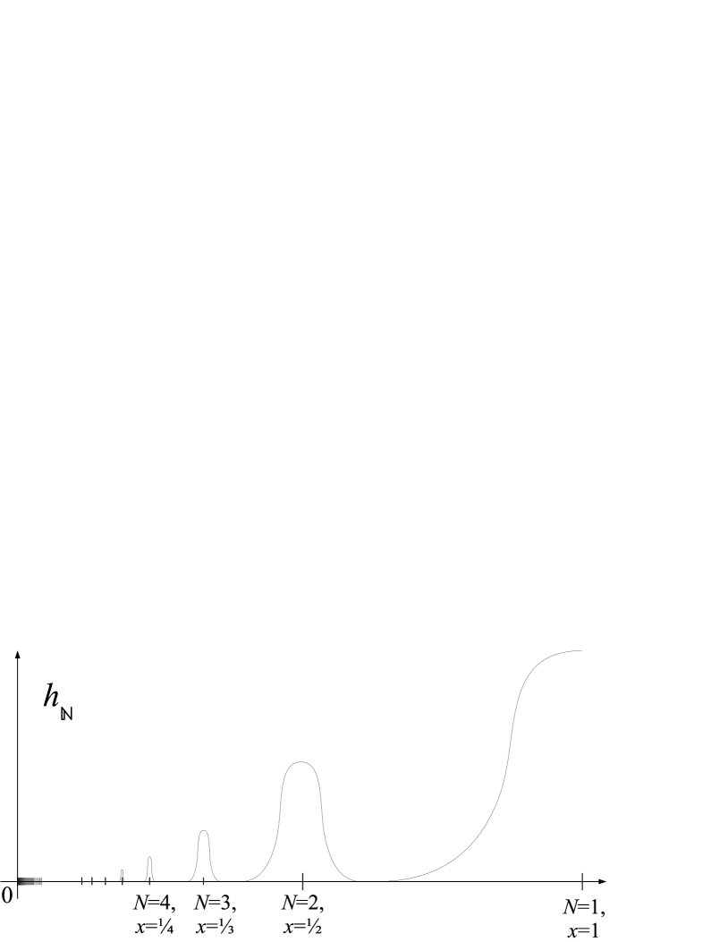
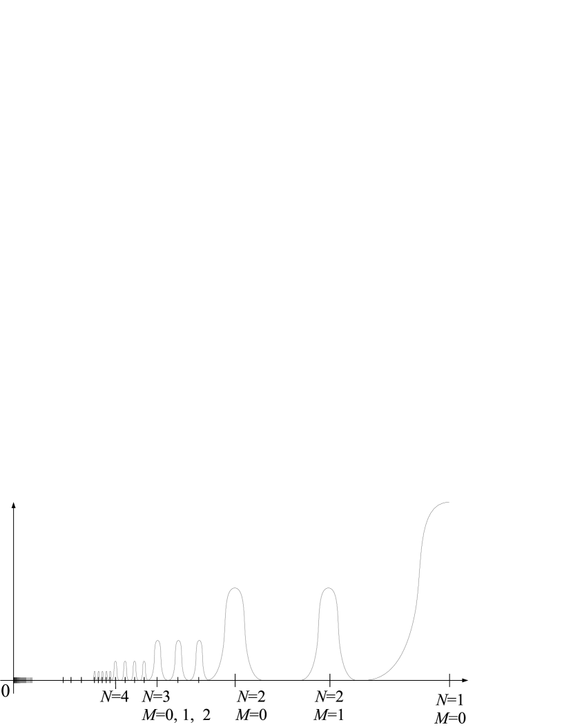
Figure 2: Encoding decision problems into smooth functions: Illustrating the proof of Example 1.14.

As already pointed out, this notion of complexity may be trivial for some $\xi$ and $\upsilon$. (Meta-)Conditions on the representations under consideration are devised in [Weih03]. We conclude this subsection by recalling the construction underlying [Ko91, Theorem 3.7] of a polytime computable smooth $h:[0;1]\to[0;1]$ for which the function $\operatorname{Max}(h):[0;1]\to[0;1]$ is not polytime unless $\mathcal{P}=\mathcal{NP}$:

Example 1.14

1. Recall from Example 1.6 that the function

   $$h_{1}(x)\;:=\;\exp\big{(}\tfrac{4x^{2}}{4x^{2}-1}\big{)}\quad\text{ for }|x|\leq\tfrac{1}{2},\qquad h_{1}(x):=0\quad\text{ for }|x|\geq\tfrac{1}{2}$$

   is smooth on $[-1;1]$ and vanishes outside $\big{[}-\tfrac{1}{2};\tfrac{1}{2}\big{]}$. Similarly, the scaled and shifted $h_{N}(x):=h(2N^{2}\cdot x-2N)/N^{\ln N}$ is smooth with maximum $\exp(-\ln^{2}N)$ attained at $x=1/N$ and vanishes outside $\big{[}\tfrac{1}{N}-\tfrac{1}{4N^{2}};\tfrac{1}{N}+\tfrac{1}{4N^{2}}\big{]}$. Note that $\tfrac{1}{N}-\tfrac{1}{4N^{2}}\geq\tfrac{1}{N+1}+\tfrac{1}{4(N+1)^{2}}$ holds for $N\in\mathbb{N}$, hence $h_{N}$ has support disjoint to that of $h_{N^{\prime}}$ whenever $N,N^{\prime}\in\mathbb{N}$ are distinct. Moreover, for every $j\in\mathbb{N}_{0}$, $h_{N}^{(j)}(x)=h_{1}^{(j)}(2N^{2}\cdot x-2N)\cdot N^{2j}/N^{\ln N}\to 0$ uniformly in $x$ as $N\to\infty$. Therefore (and abusing notation) the function $h_{L}:=\sum_{N\in L}h_{N}:[0;1]\to[0;1]$ is smooth for every $L\subseteq\mathbb{N}$; and the question “$N\in L$?” reduces to evaluating $h_{L}(1/N)$ up to absolute error $2^{-n}$ for $n:=(\ln N)^{2}\cdot\log e$ polynomial in the length of $N$: Modulo polytime, the computational complexity of $h_{L}$ coincides with that of $L$ as a discrete binary decision problem.

2. We argue that also the computational complexity of $\operatorname{Max}(h_{L})$ coincides (modulo polytime) with that of $L$. To this end note that, for $x\leq 1$, $\exp(x/2)\leq 1+x$ and thus $\ln(1+x)\geq x/2$:

   $$\ln^{2}(N+1)\ln^{2}(N) = \big{(}\ln(N+1)+\ln(N)\big{)}\cdot\ln\big{(}1+\tfrac{1}{N}\big{)}\;\geq\;2\ln(N)/(2N)\geq 1/N\enspace,$$

   $$e^{-\ln^{2}(N)}-e^{-\ln^{2}(N+1)} = e^{-\ln^{2}N}\cdot\Big{(}1-e^{-\big{(}\ln^{2}(N+1)-\ln^{2}(N)\big{)}}\Big{)}$$

   $$\geq e^{-\ln^{2}N}\cdot\big{(}1-e^{1/N}\big{)}\;\geq\;e^{-\ln^{2}N-\ln N-1}$$

   because $1-e^{-1/N}\geq\tfrac{1}{eN}=e^{-\ln N-1}$. Note observe that $\operatorname{Max}\big{(}h_{L}\big{)}(1/N)=\exp\big{(}-\ln^{2}(N)\big{)}$ holds if $N\in L$, whereas $\operatorname{Max}\big{(}h_{L}\big{)}(1/N)\leq\exp\big{(}-\ln^{2}(N+1)\big{)}$ if $N\not\in L$. And the above estimates demonstrate that both cases can be distinguished by evaluating $\operatorname{Max}\big{(}h_{L}\big{)}(1/N)$ up to absolute error $2^{-n}$ for $n:=\mathcal{O}(\ln^{2}N)$ polynomial in the binary length of $N$.

3. Slightly more generally consider

   $$L\;\subseteq\;\{(N,M):N\in\mathbb{N},\mathbb{N}_{0}\ni M<N\},\qquad K\;:=\;\{N:\exists M:(N,M)\in L\}$$

   and observe that the condition $M<N$ on integer values implies the binary length of $M$ to be bounded by that of $N$ from which in turn follows $M<2N$; hence this condition can be met by ‘padding’ $N$ with polynomially many dummy digits in order to obtain a $\mathcal{NP}$–complete $K$ with $L\in\mathcal{P}$. Now let

   $$h_{N,M}(x)\;:=\;h_{1}(3N^{3}\cdot x-3N^{2}-M)/N^{\ln N},\qquad h_{L}:=\sum\nolimits_{(N,M)\in L}h_{N,M}$$

   and note as in a) that $h_{N,M}$ is smooth with maximum $\exp(-\ln^{2}N)$ attained at $x_{N,M}:=\tfrac{1}{N}+\tfrac{M}{3N^{3}}$ and vanishes outside $\Big{[}\frac{1}{N}+\frac{M-1/2}{3N^{3}};\frac{1}{N}+\frac{M+1/2}{3N^{3}}\Big{]}$. Moreover $\tfrac{1}{N}-\tfrac{1}{6N^{3}}\geq\tfrac{1}{N+1}+\tfrac{N}{3(N+1)^{3}}+\tfrac{1}{6(N+1)^{3}}$ shows that $h_{N,M}$ has support disjoint to that of $h_{N^{\prime},M^{\prime}}$ for distinct $(N,M),(N^{\prime},M^{\prime})$ with $M<N$ and $M^{\prime}<N^{\prime}$. Hence $h_{L}$ is polytime computable iff $L\in\mathcal{P}$. On the other hand it holds $\operatorname{Max}\big{(}h_{L}\big{)}(x_{N,N-1})=\exp\big{(}-\ln^{2}(N)\big{)}$ in case $N\in K$ and $\operatorname{Max}\big{(}h_{L}\big{)}(x_{N,N-1})\leq\exp\big{(}-\ln^{2}(N+1)\big{)}$ in case $N\not\in K$: both distinguishable by evaluating $\big{(}h_{L}\big{)}(x_{N,N-1})$ up to absolute error polynomial in the binary length of $N$. Therefore polytime evaluation of $\operatorname{Max}(h_{L})$ implies $K\in\mathcal{P}=\mathcal{NP}$.

1.3 Uniformly Computing Real Operators

In common terminology, an operator maps functions to functions; and a functional maps (real) functions to (real) numbers. In order to define computability (Remark 1.10c) and complexity (Definition 1.13b), it suffices to choose some representation of the function space to operate on: for integration and maximization that is the set $C[0;1]$ of continuous $f:[0;1]\to\mathbb{R}$. In view of Section 1.2, (b1) provides a reasonable such encoding (which we choose to call $[\rho_{\text{\rm dy}}\!\to\!\rho_{\text{\rm dy}}]$): concerning computability, but not for the refined view of complexity. In fact any uniform complexity theory of real operators is faced with

Problem 1.15

1. Even restricted to $C([0;1],[0;1])$, that is to continuous functions $f:[0;1]\to[0;1]$, the maps $f:[0;1]\ni x\mapsto f(x)\in[0;1]$ are not computable within time uniformly bounded in terms on the output error $2^{-n}$ only.

2. Restricted further to the subspace $\operatorname{Lip}_{1}([0;1],[0;1])$ of non-expansive such functions (i.e. additionally satisfying $|f(x)-f(y)|\leq|x-y|$), there is no representation (i.e. a surjection $\delta$ defined on some subset of $\{\textup{{0}},\textup{{1}}\}^{\omega}$) rendering evaluation or integration computable in uniform time subexponential in $n$.

Figure 3: Encoding the binary strings 1011 and 1001 into 1-Lipschitz functions $f,g$ with $\|f-g\|$ not too small

Proof

1. follows from Fact 1.11 since there exist arbitrarily ‘steep’ continuous functions $f:[0;1]\to[0;1]$.

2. Technically speaking, the so-called width of this function space is exponential [Weih03, Example 6.10]. More elementarily, Figure 3 demonstrates how to encode each $\vec{b}\in\{\textup{{0}},\textup{{1}}\}^{n}$ into a non-expansive function $f_{\vec{b}}:[0;1]\to[0;1]$ with $\|f_{\vec{b}}-f_{\vec{a}}\|\geq 2^{-n}$ for $\vec{b}\neq\vec{a}$. These $2^{2^{n}}$ functions thus can be told apart by evaluation up to error $2^{-n-2}$ at arguments $(k+1/2)\cdot 2^{-n}$, $0\leq k<2^{n}$; alternatively by integrating from $k\cdot 2^{-n}$ to $(k+1)\cdot 2^{-n}$. Any algorithm doing so within time $\leq t(n)$ can read at most the first $N:=t(n)$ bits of its given $\delta$–name. However there are only $2^{N}$ different initial segments of putative such names. It thus follows $t(n)\geq 2^{\Omega(n)}$. ∎

[Ko91, Definition 2.37] solves Problem 1.15a) by permitting the running time to depend polynomially on both $n$ and $f$’s modulus of continuity as a second (order) parameter, similar to Example 1.7b). We provide an alternative perspective to this resolution in Subsection 2 below.

1.4 Type-3 Complexity Theory

Concerning Problem 1.15b), encodings as strings with sequential access seem a restriction compared to actual computers random access memory and subroutine calls providing on-demand information: Given (an algorithm computing) some $f$, this permits to approximate the value $f(a)$ for $a\in\mathbb{D}_{n+1}$ up to error $2^{-n}$ without having to (calculate and) skip over all order $2^{n}$ values $f(a^{\prime})$, $a^{\prime}\in\mathbb{D}_{n^{\prime}}$, $n^{\prime}<n$. This can be taken into account by modelling access to $f$ via oracles that, given $a\in\mathbb{D}_{n+1}$, report $b\in\mathbb{D}_{n+1}$ with $|b-f(a)|\leq 2^{-n}$; equivalently: using not infinite strings (i.e. total mappings $\{1\}^{*}\to\{\textup{{0}},\textup{{1}}\}$) but string functions (i.e. total mappings $\{\textup{{0}},\textup{{1}}\}^{*}\to\{\textup{{0}},\textup{{1}}\}^{*}$) to encode $f$. And indeed [KaCo10] resolves Problem 1.15b) by extending TTE (Remark 1.8) and generalizing Cantor space as the domain of a representation to (a certain subset of) Baire space:

Definition 1.16

1. Let $\mathcal{R}$ denote the set of all total functions $\psi:\{\textup{{0}},\textup{{1}}\}^{*}\to\{\textup{{0}},\textup{{1}}\}^{*}$ length-monotone in the sense of verifying

   $$|\vec{v}|\;\leq\;|\vec{w}|\quad\Rightarrow\quad|\psi(\vec{v})|\;\leq\;|\psi(\vec{w})|\enspace.$$ (4)

   Write $|\psi|:\mathbb{N}\to\mathbb{N}$ for the (thus well-defined) mapping $|\vec{w}|\mapsto|\psi(\vec{w})|$.

2. A second-order representation for a space $X$ is a surjective partial mapping $\tilde{\xi}:\subseteq\mathcal{R}\to X$.

3. Any ordinary representation $\xi:\subseteq\{\textup{{0}},\textup{{1}}\}^{\omega}\to X$ induces a second-order representation $\tilde{\xi}$ as follows: Whenever $\bar{\sigma}$ is a $\xi$–name of $x$, then $\psi:\{\textup{{0}},\textup{{1}}\}^{*}\ni\vec{v}\mapsto\sigma_{|\vec{v}|}\in\{\textup{{0}},\textup{{1}}\}$ is a $\tilde{\xi}$–name of said $x$.

4. Let $\tilde{\xi}:\subseteq\mathcal{R}\to X$ and $\tilde{\upsilon}:\subseteq\mathcal{R}\to Y$ be second-order representations. The product $\tilde{\xi}\times\tilde{\upsilon}$ is the second-order representation whose names for $(x,y)\in X\times Y$ consist of mappings

   $$\textup{{0}}\,\vec{w}\;\mapsto\;\textup{{0}}^{m-|\psi_{0}(\vec{w})|}\,\textup{{1}}\,\psi_{0}(\vec{w}),\qquad\textup{{1}}\,\vec{w}\;\mapsto\;\textup{{0}}^{m-|\psi_{1}(\vec{w})|}\,\textup{{1}}\,\psi_{1}(\vec{w})$$

   where $\psi_{0}$ denote a $\tilde{\xi}$–name of $x$ and $\psi_{1}$ a $\tilde{\upsilon}$–name of $y$ and $m:=\max\{|\psi_{0}(\vec{w})|,|\psi_{1}(\vec{w})|\}$.

5. More generally, fix a injective linear-time bi-computable length-monotone mapping $\langle\,\cdot\,,\,\cdot\,\rangle:\{\textup{{0}},\textup{{1}}\}^{*}\times\{\textup{{0}},\textup{{1}}\}^{*}\to\{\textup{{0}},\textup{{1}}\}^{*}$ and an arbitrary index set $A\subseteq\{\textup{{0}},\textup{{1}}\}^{*}$ as well as second-order representations $\tilde{\xi}_{\vec{a}}:\subseteq\mathcal{R}\to X_{\vec{a}}$, $\vec{a}\in A$. The product $\prod_{\vec{a}\in A}\tilde{\xi}_{\vec{a}}$ is the second-order representation of $\prod_{\vec{a}\in A}X_{\vec{a}}$ whose names $\psi$ of $(x_{\vec{a}})_{{}_{\vec{a}\in A}}$ satisfy that $\{\textup{{0}},\textup{{1}}\}^{*}\ni\vec{v}\mapsto\psi(\langle\vec{a},\vec{v}\rangle)\in\{\textup{{0}},\textup{{1}}\}^{*}$ constitutes a $\tilde{\xi}_{\vec{a}}$–name of $x_{\vec{a}}$ for each $\vec{a}\in A$, padded with some initial $\textup{{0}}^{*}\,\textup{{1}}$ to attain common length $|\psi|(n)$ on all arguments of length $n=|\langle\vec{a},\vec{v}\rangle|$.

6. An oracle Type-2 Machine $\mathcal{M}^{\psi}$ may write onto its query tape some $\vec{w}\in\{\textup{{0}},\textup{{1}}\}^{*}$ which, when entered the designated query state, will be replaced with $\vec{v}:=\psi(\vec{w})$.
   (We implicitly employ some linear-time bicomputable self-delimited encoding on this tape such as $(w_{1},\ldots,w_{n})\mapsto\textup{{1}}\,w_{1}\,\textup{{1}}\,w_{2}\,\ldots\textup{{1}}\,w_{n}\,\textup{{0}}$.)

7. $\mathcal{M}^{?}$ computes a partial mapping $\tilde{F}:\subseteq\{\textup{{0}},\textup{{1}}\}^{\omega}\times\mathcal{R}\to\{\textup{{0}},\textup{{1}}\}^{\omega}$ if, for every $(\bar{\sigma},\psi)\in\operatorname{dom}(\tilde{F})$, $\mathcal{M}^{\psi}$ on input $\bar{\sigma}$ produces $\tilde{F}(\bar{\sigma},\psi)$.
   $\mathcal{M}^{?}$ computes a partial mapping $\tilde{G}:\subseteq\{\textup{{0}},\textup{{1}}\}^{\omega}\times\mathcal{R}\to\mathcal{R}$ if, for every $(\bar{\sigma},\psi)\in\operatorname{dom}(\tilde{G})$ and every $\vec{v}\in\{\textup{{0}},\textup{{1}}\}^{*}$, $\mathcal{M}^{\psi}$ on input $(\bar{\sigma},\vec{v})$, $\vec{v}\in\{\textup{{0}},\textup{{1}}\}^{*}$, produces $\tilde{G}\big{(}\bar{\sigma},\psi\big{)}(\vec{v})\in\{\textup{{0}},\textup{{1}}\}^{*}$; cmp. Figure 4a).

8. For ordinary representation $\xi$ of $X$ and second-order representation $\tilde{\upsilon}$ of $Y$ and ordinary representation $\zeta$ of $Z$, $\tilde{F}:\subseteq\{\textup{{0}},\textup{{1}}\}^{\omega}\times\mathcal{R}\to\{\textup{{0}},\textup{{1}}\}^{\omega}$ is a $(\xi,\tilde{\upsilon},\zeta)$–realizer of a (possibly partial and multivalued) function $f:\subseteq X\times Y\rightrightarrows Z$  iff, for every $(x,y)\in\operatorname{dom}(f)$ and every $\xi$–name $\bar{\sigma}$ of $x$ and every $\tilde{\upsilon}$–name of $y$, $\tilde{F}(\psi)$ is a $\zeta$–name of some $z\in f(x,y)$.
   For second-order representation $\tilde{\zeta}$ of $Z$, $\tilde{G}:\subseteq\{\textup{{0}},\textup{{1}}\}^{\omega}\times\mathcal{R}\to\mathcal{R}$ is a $(\xi,\tilde{\upsilon},\tilde{\zeta})$–realizer of $f$ if, for every $(x,y)\in\operatorname{dom}(f)$ and every $\xi$–name $\bar{\sigma}$ of $x$ and every $\tilde{\upsilon}$–name of $y$, $\tilde{G}(\psi)$ is a $\tilde{\zeta}$–name of some $z\in f(x,y)$.

From a mere computability point of view, each representation on Baire space is equivalent to one on Cantor space [Weih00, Exercise 3.2.17]. Concerning complexity, an approximation of $\psi\in\mathcal{R}$ up to error $2^{-n}$ naturally consists of the restriction $\psi|_{\{0,1\}^{n}\}}$; cmp. [KaCo96, Definition 4.1]. Recall that any $\psi:\{\textup{{0}},\textup{{1}}\}^{*}\to\{\textup{{0}},\textup{{1}}\}^{*}$ may w.l.o.g. be presumed self-delimiting and then redefined such as to satisfy Equation (4) by appropriately ‘padding’. We require every $\tilde{\xi}$–name $\psi$ to be total, but often the information on $x$ is contained in some restriction of $\psi$. Note that an oracle query $\vec{w}\mapsto\vec{v}:=\psi(\vec{w})$ according to Definition 1.16f) may return a (much) longer answer for some argument $\psi$ than for some other $\psi^{\prime}$; so in order to be able to even read such a reply for some fixed $n$, the permitted running time bound should involve both $n$ and $|\psi|$. Since only the former is a number, this naturally involves a concept already introduced in [Mehl76]:

Definition 1.17

1. A second-order polynomial $P=P(n,\ell)$ is a term composed from variable symbol $n$, unary function symbol $\ell()$, binary function symbols $+$ and $\times$, and positive integer constants.

2. Let $T:\mathbb{N}\times\mathbb{N}^{\mathbb{N}}\to\mathbb{N}$ be arbitrary. Oracle machine $\mathcal{M}^{?}$ computing $\tilde{F}:\subseteq\{\textup{{0}},\textup{{1}}\}^{\omega}\times\mathcal{R}\to\{\textup{{0}},\textup{{1}}\}^{\omega}$ according to Definition 1.16f+g) operates in time $T$ if, for every $(\bar{\sigma},\psi)\in\operatorname{dom}(\tilde{F})$ and every $n\in\mathbb{N}$, $\mathcal{M}^{\psi}$ on input $\bar{\sigma}$ produces the $n$-th output symbol within at most $T(n,|\psi|)$ steps.
   $\mathcal{M}^{?}$ computing $\tilde{G}:\subseteq\{\textup{{0}},\textup{{1}}\}^{\omega}\times\mathcal{R}\to\mathcal{R}$ operates in time $T$ if, for every $(\bar{\sigma},\psi)\in\operatorname{dom}(\tilde{G})$, $\mathcal{M}^{\psi}$ on input $\vec{v}\in\{\textup{{0}},\textup{{1}}\}^{n}$ makes at most $T(n,|\psi|)$ steps.

3. For ordinary representations $\xi$ of $X$ and $\zeta$ of $Z$ as well as second-order representations $\tilde{\upsilon}$ of $Y$ and $\tilde{\zeta}$ of $Z$, a (possibly partial and multivalued) function $f:\subseteq X\times Y\rightrightarrows Z$ is $(\xi,\tilde{\upsilon},\zeta)$–computable in time $T$  iff  $f$ has a $(\xi,\tilde{\upsilon},\zeta)$–realizer $\tilde{F}$ computable in this time;
   similarly for $(\xi,\tilde{\upsilon},\tilde{\zeta})$–computability.

4. Second-order polytime computability means computability in time $P$ for some second-order polynomial $P$.

5. An ordinary representation $\xi$ of $X$ polytime reduces to an ordinary or second-order representation $\tilde{\upsilon}$ of $X$ (written $\tilde{\xi}\preceq_{\text{\rm p}}\tilde{\xi}$) if the identity $\operatorname{id}:X\to X$ is $(\tilde{\xi},\tilde{\upsilon})$–computable within (first-order) polytime.
   A second-order representation $\tilde{\xi}$ of $X$ (second-order) polytime reduces to an ordinary or second-order representation $\tilde{\upsilon}$ of $X$ (written $\tilde{\xi}\preceq_{\text{\rm P}}^{2}\tilde{\xi}$) if the identity $\operatorname{id}:X\to X$ is $(\tilde{\xi},\tilde{\upsilon})$–computable in second-order polytime.
   (Second-order) polytime equivalence means that also the converse(s) hold(s).

‘Long’ arguments $\psi$ are thus granted more time to operate on; see Remark 1.20 below. Every ordinary (i.e. first-order) bivariate polynomial $p(n,k)$ obviously can be seen as a second-order polynomial by identifying $k\in\mathbb{N}$ with the constant function $\ell(n)\equiv k$; but not conversely, as illustrated with the example $n\cdot\ell\Big{(}n^{5}+\big{(}\ell(n^{2})\big{)}^{2}\Big{)}$. Second-order polynomials also constitute the second-level of a Grzegorczyk Hierachy on functionals of finite type arising naturally as bounds in proof-mining [Kohl96, middle of p.33]; cmp. also [ProofMining, §A] and [TeZi10]. In fact on arguments $\ell$ polynomial of unbounded degree, only second-order polynomials satisfy closure under both kinds of composition:

$$\big{(}Q\circ P\big{)}(n,\ell)\;\;:=\;\;Q\big{(}P(n,\ell),\ell\big{)}\quad\text{ and }\quad\big{(}Q\bullet P\big{)}(n,\ell)\;\;:=\;\;Q\big{(}n,P(\cdot,\ell)\big{)}\enspace.$$ (5)

Second-order representations induced by ordinary ones on the other hand basically use only string functions $\psi$ on unary arguments with binary values, i.e. of length $|\psi|\equiv 1$; and these indeed recover first-order TTE complexity:

Observation 1.18

1. Any bivariate ordinary polynomial $p(n,m)$ can be bounded by some univariate polynomial in $n+m$. Any bivariate second-order polynomial $P\big{(}n,\ell(),k()\big{)}$ — that is a term composed from $n$, $\ell()$, $k()$, $+$, $\times$, and $1$ — can be bounded by some $Q\big{(}n,\ell()+k()\big{)}$.

2. Let $P=P(n,\ell)$ denote a second-order polynomial and $\ell$ a monic linear function with offset $k$, i.e., $\ell(n)=n+k\in\mathbb{N}$. Then $P(n,\ell)$ boils down to an ordinary bivariate polynomial in $n$ and $k$. In particular, $P(0,\equiv k)$ is a polynomial in $k$.

3. More generally, fix $d\in\mathbb{N}$ and consider the module $\mathbb{N}_{d}$ of polynomials $\ell$ over $\mathbb{N}$ of degree less than $d$: $\ell(n)=\sum_{j<d}k_{j}n^{j}$.
   Subject to this restriction, every second-order polynomial $P=P(n,\ell)$ can be bounded by a univariate polynomial in $n+k_{0}+\cdots+k_{d-1}$.

4. Let $\xi$ denote an ordinary representation of $X$ and $\tilde{\xi}$ its induced second-order representation. Then $\xi$ reduces to $\tilde{\xi}$ within (first-order) polytime: $\xi\preceq_{\text{\rm p}}\tilde{\xi}$;
   and $\tilde{\xi}$ reduces to $\xi$ within first-order polytime: $\tilde{\xi}\preceq_{\text{\rm P}}^{2}\xi$.

5. Let $\xi$ and $\upsilon$ denote ordinary representations of $X$ and $Y$ with induced second-order representations $\tilde{\xi}$ and $\tilde{\upsilon}$, respectively. Then the second-order representation $\widetilde{\xi\times\upsilon}$ of $X\times Y$ induced by $\xi\times\upsilon$ is polytime equivalent to $\tilde{\xi}\times\tilde{\upsilon}$.

6. For each $j\in\mathbb{N}$ let $\xi_{j}$ denote an ordinary representation of $X_{j}$ and $\tilde{\xi}_{\textup{{1}}^{j}}$ its induced second-order representation. Then the second-order representation $\widetilde{\prod_{j}\xi_{j}}$ of $\prod_{j}X_{j}$ is polytime equivalent to $\prod_{j}\tilde{\xi}_{\textup{{1}}^{j}}$, that is, with respect to indices encoded in unary.

Proof

a+b+c) are immediate.

1. Given $\bar{\sigma}$ and $\vec{v}$, it is easy to return $\sigma_{|\vec{v}|}$, thus $(\xi,\tilde{\xi})$–computing $\operatorname{id}_{X}$ within polynomial time;
   similarly for the converse, observing that $\tilde{\xi}$–names $\psi$ have constant length, see b).

2. Observe that a $\widetilde{\xi\times\upsilon}$–name $\psi$ of $(x,y)$ has $|\psi|\equiv 1$ and $\xi\big{(}\psi(\textup{{1}}^{2n})_{{}_{n}}\big{)}=x$ and $\upsilon\big{(}\psi(\textup{{1}}^{2n+1})_{{}_{n}}\big{)}=y$; while a $\tilde{\xi}\times\tilde{\upsilon}$–name $\psi$ has $|\psi|\equiv 1$ and $\xi\big{(}\psi(\textup{{0}}\,\textup{{1}}^{n})_{{}_{n}}\big{)}=x$ and $\upsilon\big{(}\psi(\textup{{1}}\,\textup{{1}}^{n})_{{}_{n}}\big{)}=y$.

3. A $\widetilde{\prod_{j}\xi_{j}}$–name of $(x_{j})$ has $|\psi|\equiv 1$ and $\xi_{j}\big{(}\psi(\textup{{1}}^{\langle n,j\rangle})_{{}_{n}}\big{)}=x_{j}$; while a $\big{(}\prod_{j}\tilde{\xi}_{\textup{{1}}^{j}}\big{)}$–name $\psi$ has $|\psi|\equiv 1$ and $\xi_{j}\big{(}\psi(\langle\textup{{1}}^{j},\textup{{1}}^{n}\rangle)_{{}_{n}}\big{)}=x_{j}$ ∎

As with ordinary representations, not every choice of $\tilde{\xi}$ and $\tilde{\upsilon}$ leads to a sensible notion of complexity. Concerning the case of continuous functions on Cantor space and on the real interval $[0;1]$, we record and report from [KaCo10, §4.3]:

Example 1.19

1. Define a second-order representation $\rho_{\text{\rm dy}}^{\mathbb{D}}:\subseteq\mathbb{B}\to C[0;1]$ as follows:
   Length-monotone $\psi:\{\textup{{0}},\textup{{1}}\}^{*}\to\{\textup{{0}},\textup{{1}}\}^{*}$ is a $\rho_{\text{\rm dy}}^{\mathbb{D}}$–name of bounded partial $f:\subseteq[0;1]\to\mathbb{R}$

   $$\text{iff}\quad\forall\vec{w}\in\{\textup{{0}},\textup{{1}}\}^{*}:\qquad\Big{(}\operatorname{dom}(f)\cap\operatorname{ball}\big{(}\operatorname{bin}(\vec{w})/2^{|\vec{w}|+1},2^{-|\vec{w}|}\big{)}\neq\emptyset\quad\Rightarrow\\ \exists x\in\operatorname{dom}(f)\cap\operatorname{ball}\big{(}\operatorname{bin}(\vec{w})/2^{|\vec{w}|+1},2^{-|\vec{w}|}\big{)}:\;\big{|}\operatorname{bin}\big{(}\psi(\vec{w})\big{)}/2^{|\vec{w}|+1}-f(x)\big{|}\leq 2^{-|\vec{w}|}\Big{)}\enspace.$$

   It holds $n+\log\|f\|_{\infty}\leq|\psi|(n)\leq C_{\psi}+n$ for all $n\in\mathbb{N}$ and some $C_{\psi}\in\mathbb{N}$.

2. For $\ell\geq 0$, let $\operatorname{Lip}_{\ell}[0;1]:=\big{\{}f:[0;1]\to\mathbb{R},|f(x)-f(y)|\leq\ell\cdot|x-y|\big{\}}$ and $\operatorname{Lip}[0;1]:=\bigcup_{\ell}\operatorname{Lip}_{\ell}[0;1]$ the class of (globally) Lipschitz-continuous functions. Define a $\big{(}\rho_{\text{\rm dy}}^{\mathbb{D}}+\operatorname{binary}(\operatorname{Lip})\big{)}$–name of $f\in\operatorname{Lip}[0;1]$ to be a mapping $\{\textup{{0}},\textup{{1}}\}^{*}\ni\vec{w}\mapsto\langle\operatorname{bin}(\ell),\psi(\vec{w})\rangle\in\{\textup{{0}},\textup{{1}}\}^{*}$, where $\psi$ denotes a $\rho_{\text{\rm dy}}^{\mathbb{D}}$–name of $f$ and $\ell\in\mathbb{N}$ some Lipschitz constant to it. It thus holds $n+\log\|f\|_{\infty}+\log\ell\leq|\psi|(n)\leq n+C^{\prime}_{\psi}$.

3. Define a $[\widetilde{\rho_{\text{\rm dy}}\!\!\!\to\!\!\rho_{\text{\rm dy}}}]$–name (in [KaCo10] called a $\delta_{{}_{\Box}}$–name) $\psi$ of $f\in C[0;1]$ to be a mapping $\{\textup{{0}},\textup{{1}}\}^{*}\;\ni\;\vec{w}\;\mapsto\;\textup{{1}}^{\mu(|\vec{w}|}\,\textup{{0}}\,\psi(\vec{w})\;\in\{\textup{{0}},\textup{{1}}\}^{*}$, where $\psi$ denotes a $\rho_{\text{\rm dy}}^{\mathbb{D}}$–name of $f$ and $\mu:\mathbb{N}\to\mathbb{N}$ is a modulus of uniform continuity to it. It thus holds $\mu(n)+n+\log\|f\|_{\infty}\leq|\psi|(n)\leq n+C^{\prime\prime}_{\psi}$.

4. Recall that the identity $\operatorname{id}$ is the standard representation of Cantor space. Inspired by [Roes11, Definition 3.6.1], consider the following second-order (multi-) representation of the space $\operatorname{UC}(\subseteq\{\textup{{0}},\textup{{1}}\}^{\omega}\to\{\textup{{0}},\textup{{1}}\}^{\omega})$ of uniformly continuous partial functions on Cantor space:
   A $\tilde{\eta}$–name of $F$ maps $\textup{{1}}^{n}\,\textup{{0}}\,\vec{x}\in\{\textup{{0}},\textup{{1}}\}^{*}$ to some $\textup{{1}}^{m}\,\textup{{0}}\,\vec{y}$ such that $d\big{(}F(\bar{x}),\vec{y}\big{)}\leq 2^{-n}$ for all $\bar{x}\in\operatorname{dom}(F)$ with $d(\bar{x},\vec{x})\leq 2^{-m}$. Here $d(\bar{x},\vec{y})=\max\{2^{-j}:x_{j}\neq y_{j}\;\vee\;j>|\vec{y}|\}$ induces the the metric on Cantor space.

5. $[\widetilde{\rho_{\text{\rm dy}}\!\!\!\to\!\!\rho_{\text{\rm dy}}}]$ is computably equivalent to $[\rho_{\text{\rm dy}}\!\to\!\rho_{\text{\rm dy}}]$.
   More precisely the evaluation functional $C[0;1]\times[0;1]\ni(f,x)\mapsto f(x)\in\mathbb{R}$ is $\big{(}[\widetilde{\rho_{\text{\rm dy}}\!\!\!\to\!\!\rho_{\text{\rm dy}}}]\times\widetilde{\rho}_{\text{\rm dy}},\widetilde{\rho}_{\text{\rm dy}}\big{)}$–computable in second-order polytime;
   and the evaluation functional $\operatorname{UC}(\subseteq\{\textup{{0}},\textup{{1}}\}^{\omega}\to\{\textup{{0}},\textup{{1}}\}^{\omega})\times\{\textup{{0}},\textup{{1}}\}^{\omega}\ni(F,\bar{x})\mapsto F(\bar{x})\in\{\textup{{0}},\textup{{1}}\}^{\omega}$ is $\big{(}\tilde{\eta}\times\tilde{\operatorname{id}},\tilde{\operatorname{id}}\big{)}$–computable in second-order polytime.

6. It holds $\rho_{\text{\rm dy}}^{\mathbb{D}}+\operatorname{binary}(\operatorname{Lip})\preceq_{\text{\rm P}}^{2}[\widetilde{\rho_{\text{\rm dy}}\!\!\!\to\!\!\rho_{\text{\rm dy}}}]\big{|}^{\operatorname{Lip}[0;1]}$ with $\operatorname{Lip}[0;1]\subseteq C[0;1]$;
   but $[\widetilde{\rho_{\text{\rm dy}}\!\!\!\to\!\!\rho_{\text{\rm dy}}}]\big{|}^{\operatorname{Lip}[0;1]}\not\preceq_{\text{\rm P}}^{2}\rho_{\text{\rm dy}}^{\mathbb{D}}+\operatorname{binary}(\operatorname{Lip})$.

7. For arbitrary closed $K\subseteq\{\textup{{0}},\textup{{1}}\}^{\omega}$, every total polytime-computable $F:K\to\{\textup{{0}},\textup{{1}}\}^{\omega}$ admits a polytime-computable $\tilde{\eta}$–name $\psi$. Similarly, to every ‘family’ of total functionals $\Lambda:C[0;1]\times[0;1]\to C[0;1]$ $([\widetilde{\rho_{\text{\rm dy}}\!\!\!\to\!\!\rho_{\text{\rm dy}}}]\times\widetilde{\rho}_{\text{\rm dy}},\widetilde{\rho}_{\text{\rm dy}})$–computable in second-order polytime, there exists a second-order polytime $([\widetilde{\rho_{\text{\rm dy}}\!\!\!\to\!\!\rho_{\text{\rm dy}}}],[\widetilde{\rho_{\text{\rm dy}}\!\!\!\to\!\!\rho_{\text{\rm dy}}}])$–computable operator $\mathbb{O}:C[0;1]\to C[0;1]$ such that $\Lambda(f,x)=\mathcal{O}\big{(}f\big{)}(x)$ holds for all $f$ and all $x$.

Concerning a), each $f\in C[0;1]$ is indeed bounded; hence the output of $\psi$ on $\{\textup{{0}},\textup{{1}}\}^{n}$ can be padded with leading zeros (as opposed to Remark 1.8e) to $\mathcal{O}(\log\|f\|_{\infty})$ binary digits before the point and $n$ after. On the other hand, $\rho_{\text{\rm dy}}^{\mathbb{D}}$ alone lacks a bound on the slope of $f$ necessary to evaluate it on non-dyadic arguments and leads to the representations in b) and c).
Regarding d), note that the mapping $\textup{{1}}^{n}\,\textup{{0}}\,\vec{x}\to\textup{{1}}^{m}$ yields a local modulus of continuity to $F$; and the uniform continuity prerequisite again ensures that $m=m(n,\vec{x})$ can be chosen to depend only on $n$ and $|\vec{x}|$, thus yielding a length-monotone string function $\psi$.
In e), functions with ‘large’ modulus of continuity and/or ‘large’ values that might take ‘long’ to evaluate (recall Example 1.12) necessarily have $[\widetilde{\rho_{\text{\rm dy}}\!\!\!\to\!\!\rho_{\text{\rm dy}}}]$–names $\psi$ with ‘large’ $|\psi|$. Explicitly on Cantor space, given $\bar{x}$ and $n$, invoke the oracle on $\textup{{1}}^{n}$ and on finite initial segments $\vec{x}$ of $\bar{x}$ of increasing length $m^{\prime}=1,2,\ldots$ until the reported $\textup{{1}}^{m}\,\textup{{0}}\,\vec{y}$ satisfies $m\leq m^{\prime}$, then print $\vec{y}$: This asserts $d\big{(}F(\bar{x}),\vec{y}\big{)}\leq 2^{-n}$ and takes $\operatorname{poly}(m,n)$ steps, that is, second-order polytime. The real case proceeds even more directly by querying oracle $\psi$ for $m:=\mu(n+1)$ and then for $f(q)$ with $q\in\mathbb{D}_{m}$ and $|x-q|\leq 2^{-n-1}$.
For the polytime reduction in f), verify that $\mu(n)=n+\log\ell$ is a modulus of continuity to $f\in\operatorname{Lip}_{\ell}[0;1]$. Concerning failure of the converse, $\ell:=2^{\max_{n}\mu(n)-n}$ could (if finite) serve a Lipschitz constant to $f$ but is clearly not computable from finitely many queries to $\mu$. We postpone the formal proof to Example 2.6h).
Turning to g), computing $F$ in polytime means calculating the first $n$ digits $\vec{y}$ of $F(\bar{x})$ from $\bar{x}$ in time polynomial in $n$; and simulating this computation while keeping track of the number $m$ of digits $\vec{x}$ of $\bar{x}$ thus read essentially yields the $\tilde{\eta}$–name $\psi$. The difficulty consists in algorithmically finding some appropriate padding to obtain $\psi$ length-monotone in the sense of Equation (4). For co-r.e. $K$, such a bound is at least computable [Weih03, Theorem 5.5]; however in our non-uniform polytime setting, it constitutes some fixed polynomial and can be stored in the algorithm. For fixed $f$, the real case proceeds similarly and is easily seen to run in second-order polytime uniformly in $f$.

Remark 1.20

1. We follow [Mehl76, KaCo96, KaCo10] in defining the complexity of operators such that computations on ‘long’ arguments are granted more running time and still be considered polynomial, thus avoiding Problem 1.15a). This approach resembles [LLM01, Définition 2.1.7] where, too, computations on ‘long’ arguments are granted more time to achieve a desired output precision of $2^{-n}$; cmp. [Weih03, §7]. Note, however, that [LLM01, Définition 2.2.9] refers only to sequences of functions (cmp. Definition 1.16d) and, in spite of [LLM01, Theoréme 5.2.13], is therefore not a fully uniform notion of complexity for operators. A related concept, hereditarily polynomial bounded analysis [Kohl98, Oliv05] permits polynomially bounded quantification and thus climbing up Stockmeyer’s polynomial hierarchy.

2. Some $f\in\operatorname{Lip}_{1}[0;1]$ can be regarded

   1. on the one hand as a transformation on real numbers  and

   2. on the other hand as a point in a separable metric space.

   Both views induce ‘natural’ notions of computability and complexity (Definition 1.13). Now i) and ii) are equivalent concerning the former [Weih00, §6.1]; and so are they when equipping $\operatorname{Lip}_{1}[0;1]$ with the second-order representation $\rho_{\text{\rm dy}}^{\mathbb{D}}$; cmp. Lemma 4.9 in the journal version of [KaCo10]. Indeed it seems desirable that type conversion (the utm and smn properties) be not just computable [Weih00, Theorem 2.3.5] but within uniform polytime so (Example 1.19e+f) — and, in view of Remark 1.10b), not merely for polytime–computable functions [Ko91, Theorem 8.13].

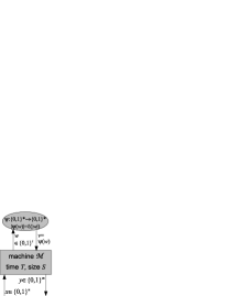
Figure 4: a) Computation of $\mathcal{M}^{\psi}$.  b) Composition of two oracle machines.

2 Parameterized Type-2 and Type-3 Complexity

As illustrated in Example 1.7a+b), real number computations sometimes may not admit running times bounded in terms of the output precision only; cmp. also the case of inversion $(0;1]\ni x\mapsto 1/x$ [Weih00, Exercise 7.2.10+Theorem 7.3.12] and of polynomial root finding [Hotz09]. Such effects are ubiquitous in numerics and captured quantitatively for instance in so-called condition numbers $k$ of matrices or, more generally, of partial functions $f:\subseteq\mathbb{R}^{d}\to\mathbb{R}$ with singularities/diverging behaviour on $\vec{x}\not\in\operatorname{dom}(f)$ [Bürg08]: in order to express and bound in terms of both $n$ and $k$ the number of iterations, i.e. basically the running time it takes in order to attain a prescribed (although, pertaining to the BSS model with equality decidable, usually relative) precision $2^{-n}$. Put differently, $k$ serves in addition to $n$ as a second (but still first-order) parameter: just like in classical complexity theory [FlGr06]. We combine both TTE complexity [Weih03, Definition 2.1] and the discrete notion of fpt–reduction:

Definition 2.1

1. Fix $F:\subseteq\{\textup{{0}},\textup{{1}}\}^{\omega}\to\{\textup{{0}},\textup{{1}}\}^{\omega}$ and $k:\operatorname{dom}(F)\to\mathbb{N}$, called parameterization of $F$. The pair $(F,k)$ is fixed-parameter tractable if there exists some recursive function $p:\mathbb{N}\to\mathbb{N}$ such that a Type-2 Machine can compute $\operatorname{dom}(F)\ni\bar{\sigma}\mapsto F(\bar{\sigma})$ within at most $n^{\mathcal{O}(1)}\cdot p\big{(}k(\bar{\sigma})\big{)}$ steps.

2. $(F,k)$ is fully polytime computable if the above running time is bounded by a polynomial in both $n$ and $k(\bar{\sigma})$, that is, if $p\in\mathbb{N}[K]$.

3. A parameterized representation or representation with parameter of a space $X$ is a tuple $(\xi,k)$ where $\xi$ denotes a representation of $X$ and $k:\operatorname{dom}(\xi)\to\mathbb{N}$ some function.

4. For a parameterized representation $(\xi,k)$ of $X$ and one $(\upsilon,\ell)$ of $Y$, let $(\xi,k)\times(\upsilon,\ell):=(\xi\times\upsilon,k+\ell)$ denote the parameterized representation of $X\times Y$. Here, $\xi\times\upsilon$ is the representation according to Remark 1.8c); and $k+\ell$ formally denotes the mapping $(\sigma_{0},\tau_{0},\sigma_{1},\tau_{1},\ldots)\mapsto k(\sigma_{0},\sigma_{1},\ldots)+\ell(\tau_{0},\tau_{1},\ldots)$.

5. For a parameterized representation $(\xi,k)$ of $X$ and a representation $\upsilon$ of $Y$, a (possibly partial and multivalued) function $f:\subseteq X\rightrightarrows Y$ is fully polytime $\big{(}(\xi,k),\upsilon\big{)}$–computable if it admits a $(\xi,\upsilon)$–realizer $F$ such that $(F,k)$ is fully polytime computable.

6. If in e) the representation $\upsilon$ for $Y$ is equipped with a parameter $\ell$ as well, call $f:\subseteq X\rightrightarrows Y$ a fixed-parameter reduction if it admits a $(\xi,\upsilon)$–realizer $F$ such that $(F,k)$ is fixed-parameter tractable and it holds $\ell\big{(}F(\bar{\sigma})\big{)}\leq k(\bar{\sigma})$.

7. Again for parameterized representations $(\xi,k)$ of $X$ and $(\upsilon,\ell)$ of $Y$, a fully polytime $\big{(}(\xi,k),(\upsilon,\ell)\big{)}$–computable $f:\subseteq X\rightrightarrows Y$ must admit a $(\xi,\upsilon)$–realizer $F$ such that $(F,k)$ is fully polytime computable while increasing the parameter at most polynomially: $\ell\circ F\leq p\circ k$ for some $p\in\mathbb{N}[K]$.

8. A parameterized representation $(\xi,k)$ of $X$ is fully polytime reducible to another parameterized representation $(\upsilon,\ell)$ of $X$ (written $(\xi,k)\preceq_{\text{\rm p}}(\upsilon,\ell)$) if $\operatorname{id}:X\to X$ is fully polytime $\big{(}(\xi,k),(\upsilon,\ell)\big{)}$–computable. Fully polytime equivalence means that also the converse holds.

Since the same point $x\in X$ may have several $\xi$–names (some perhaps more difficult to parse or process than others), also the parameter may have different values for these names in e+f+g). Note that both fixed-parameter reductions (Definition 2.1f) and fully polytime computable functions (Definition 2.1g) are closed under composition.

We did not define parameterized running times for second-order maps $\tilde{F}:\subseteq\mathcal{R}\to\mathcal{R}$: because $\mathcal{R}$, as opposed to infinite binary strings, already comes equipped with a notion of size as parameter entering in running time bounds: recall Definition 1.17b).

Remark 2.2

The above notions make also sense for other complexity classes such as polynomial space. Giving up closure under composition, Definitions 2.1a+b+e+f) can be refined quantitatively to, say, quadratic-time computability — but Definition 2.1g) becomes ambiguous: just like in both the discrete case and [LLM01, Définition 2.1.7]; cmp. [Weih03, §7].

Also, as in unparameterized TTE complexity theory, the above notion of (parameterized) complexity may be meaningless for some representations — that can be avoided by imposing additional (meta-) conditions [Weih03, §4+§6]. Example 1.7b) is now rephrased as Item a) of the following

Example 2.3

1. The exponential function on the entire real line is fully polytime $\big{(}(\rho_{\text{\rm dy}},|\rho_{\text{\rm dy}}|),\rho_{\text{\rm dy}}\big{)}$–computable, where $|\rho_{\text{\rm dy}}|:=|\,\cdot\,|\circ\rho_{\text{\rm dy}}$; recall Definition 1.9.

2. A constant parameter has no effect asymptotically: For any fixed $c$, polytime $(\xi,\upsilon)$–computability is equivalent to fully polytime $\big{(}(\xi,c),\upsilon\big{)}$–computability and to fully polytime $\big{(}(\xi,c),(\upsilon,\ell)\big{)}$–computability.
   On the other hand, and as opposed to the discrete case, not every (even total) computable $F:\{\textup{{0}},\textup{{1}}\}^{\omega}\to\{\textup{{0}},\textup{{1}}\}^{\omega}$ admits some parameterization $k$ rendering $(F,k)$ is fixed-parameter tractable.

3. Suppose $\tilde{F}:\subseteq\mathcal{R}\to\mathcal{R}$ is second-order polytime computable and has $\operatorname{dom}(\tilde{F})$ consisting only of string functions of linear length in the following sense: there exists $c\in\mathbb{N}$ and $k:\operatorname{dom}(\tilde{F})\to\mathbb{N}$ such that every $\psi\in\operatorname{dom}(\tilde{F})$ satisfies $\forall n:|\psi|(n)\leq c\cdot n+k(\psi)$. Then $\tilde{F}$ is fully polytime computable.
   The hypothesis is for instance satisfied for any $\big{(}\rho_{\text{\rm dy}}^{\mathbb{D}}+\operatorname{binary}(\operatorname{Lip}),\tilde{\upsilon}\big{)}$–realizer $\tilde{F}$ of some $\Lambda:\subseteq\operatorname{Lip}[0;1]\rightrightarrows Y$.

4. Evaluation of a given power series $\big{(}(a_{j})_{{}_{j}},z\big{)}\mapsto\sum_{j=0}^{\infty}a_{j}z^{j}$ is not $\big{(}(\rho_{\text{\rm dy}}^{2})^{\omega},\rho_{\text{\rm dy}}^{2}\big{)}$–computable, even restricted to real arguments $|x|\leq 1$ and real coefficient sequences $(a_{j})_{{}_{j}}=:\bar{a}$ of radius of convergence $R(\bar{a}):=1/\limsup_{j}|a_{j}|^{1/j}>1$.
   However when given, in addition to approximations to $\bar{a}$ and $z$, also integers $K,A$ with

   $$R\;>\;\sqrt[K]{2}\;=:\;r\qquad\text{and}\qquad\forall j:\;|a_{j}|\;\leq\;A/r^{j}\enspace,$$ (6)

   evaluation up to error $2^{-n}$ becomes uniformly computable within time polynomial in $n$, $K$, and $\log A$.
   Formally let $\pi$ denote the following representation of $C^{\omega}_{1}:=\big{\{}\bar{a}\subseteq\mathbb{C},R(\bar{a})>1\big{\}}$: A $\pi$–name of $\bar{a}$ is a $\big{(}(\rho_{\text{\rm dy}}^{2})^{\omega}\times\operatorname{binary}\times\operatorname{unary}\big{)}$–name (recall Definition 1.9e+Remark 1.8c+d) of $(\bar{a},A,K)$ satisfying Equation (6). Equipping $\pi$ with parameterization $K+\log A$ renders evaluation $(C^{\omega}_{1},[-1;1])\ni(\bar{a},x\big{)}\mapsto\sum_{j}a_{j}x^{j}$ fully polytime $\big{(}(\pi,K+\log A)\times\rho_{\text{\rm dy}},\rho_{\text{\rm dy}})$–computable.

Note that the (questionable) fully polytime computability of $\exp(x)$ in a) hinges on using as parameter the value rather than, perhaps more naturally, the binary length of (the integral part of) the argument $x$. Indeed, similarly to the discrete function $\mathbb{N}\ni x\mapsto 2^{x}$, an output having length exponential in that of the input otherwise prohibits polytime computability. A notion of parameterized complexity taking into account the output size is suggested in Definition 2.4j) below.

Proof (Example 2.3)

1. immediate.

2. A polynomial evaluated on a constant argument is again a constant.
   On the other hand the Time Hierarchy Theorem yields a binary sequence $\mathbb{N}\ni n\mapsto\tau_{n}\in\{\textup{{0}},\textup{{1}}\}$ computable but not within time polynomial in $n$; now consider the constant function $F:\{\textup{{0}},\textup{{1}}\}^{\omega}\ni\bar{\sigma}\mapsto\bar{\tau}$.

3. According to Observation 1.18a+b+c), second-order polynomials $P(n,\ell)$ on linearly bounded second-order arguments $\ell(n)\leq c\cdot n+k$ with fixed $c$ can be bounded by an ordinary polynomial in $n+k$.
   Moreover recall (Example 1.19b) that $\big{(}\rho_{\text{\rm dy}}^{\mathbb{D}}+\operatorname{binary}(\operatorname{Lip})\big{)}$–names have linear length.

4. The negative claim is folklore; cmp. e.g. [Müll95]. We defer the proof of the positive claim to Theorem 3.3a). ∎

Note that, for a parameterized representation $(\xi,k)$ of $X$ according to Definition 2.1d), a Type-2 Machine $\big{(}(\xi,k),\upsilon\big{)}$–computing some $f:X\ni x\mapsto f(x)\in Y$ is provided merely with a $\xi$–name $\bar{\sigma}$ of $x$ but not with the value $k(\bar{\sigma})$ of the parameter entering in the running time bound it is to obey. In the case of the global exponential function (Example 2.3a), an upper bound to this value is readily available as part of the given $\rho_{\text{\rm dy}}$–name of $x$. In the case of power series evaluation (Example 2.3d), on the other hand, the values of parameters $K$ and $A$ had to be explicitly provided by means of the newly designed representation $\pi$, that is by ‘enriching’ [KrMa82, p.238/239] $(\rho_{\text{\rm dy}}^{2})^{\omega}$, in order to render an otherwise discontinuous operation computable; recall also Example 1.7. Such simultaneous use of integers as both complexity parameters and discrete advice will arise frequently in the sequel and is worth a generic

Definition 2.4

1. Let $\xi$ denote an ordinary representation of $X$ and $L:X\rightrightarrows\mathbb{N}$ some total multivalued function. Then “$\xi$ with advice parameter $L$ in unary” means the following parameterized representation of $X$, denoted as $\xi+\operatorname{unary}(L)=:(\upsilon,k)$: an $\upsilon$–name of $x\in X$ is an infinite binary string $\bar{\sigma}=\textup{{1}}^{\ell}\,\textup{{0}}\,\bar{\tau}$ where $\bar{\tau}$ is a $\xi$–name of $X$ and $\ell\in L(x)$; and $k(\bar{\sigma}):=\ell$.

2. Let $\xi$ denote an ordinary representation of $X$ and $L:X\rightrightarrows\mathbb{N}$ some total multivalued function. Then “$\xi$ with advice parameter $L$ in binary” means the following parameterized representation of $X$, denoted as $\xi+\operatorname{binary}(L)=:(\upsilon,k)$: an $\upsilon$–name of $x\in X$ is an infinite binary string $\bar{\sigma}=\langle\operatorname{bin}(\ell),\bar{\tau}\rangle$ where $\bar{\tau}$ is a $\xi$–name of $X$ and $\ell\in L(x)$; and $k(\bar{\sigma}):=\log\ell$. Here, $\langle\,\cdot\,,\,\cdot\,\rangle:\{\textup{{0}},\textup{{1}}\}^{*}\times\{\textup{{0}},\textup{{1}}\}^{\omega}\to\{\textup{{0}},\textup{{1}}\}^{\omega}$ denotes some fixed injective linear-time bi-computable mapping.

3. Let $\tilde{\xi}:\subseteq\mathcal{R}\to X$ denote a second-order representation and $L:X\rightrightarrows\mathbb{N}$ some total multivalued function. Then “$\tilde{\xi}$ with advice parameter $L$ in unary” means the following second-order representation, denoted as $\tilde{\xi}+\operatorname{unary}(L)$: a name of $x\in X$ is a mapping $\{\textup{{0}},\textup{{1}}\}^{*}\ni\vec{w}\mapsto\textup{{1}}^{\ell}\,\textup{{0}}\,\psi(\vec{w})\in\{\textup{{0}},\textup{{1}}\}^{*}$ where $\psi$ is a $\tilde{\xi}$–name of $x$ and $\ell\in L\big{(}\tilde{\xi}(\psi)\big{)}$.

4. Let $\tilde{\xi}:\subseteq\mathcal{R}\to X$ denote a second-order representation and $L:X\rightrightarrows\mathbb{N}$. Then “$\tilde{\xi}$ with advice parameter $L$ in binary” means the following second-order representation, denoted as $\tilde{\xi}+\operatorname{binary}(L)$: a name of $x\in X$ is a mapping $\{\textup{{0}},\textup{{1}}\}^{*}\ni\vec{w}\mapsto\langle\operatorname{bin}(\ell),\psi(\vec{w})\rangle\in\{\textup{{0}},\textup{{1}}\}^{*}$ where $\psi$ is a $\tilde{\xi}$–name of $x$ and $\ell\in L\big{(}\tilde{\xi}(\psi)\big{)}$.

5. For a function $\tilde{F}:\subseteq\{\textup{{0}},\textup{{1}}\}^{\omega}\times\mathcal{R}\to\{\textup{{0}},\textup{{1}}\}^{\omega}$ with parameterization $k:\operatorname{dom}(\tilde{F})\to\mathbb{N}$, the pair $(\tilde{F},k)$ is fully polytime if some oracle machine $\mathcal{M}^{?}$ can compute $\tilde{F}$ according to Definition 1.17b) within time a second-order polynomial in $n+k$ and $|\psi|$;
   similarly for functions $\tilde{G}:\subseteq\{\textup{{0}},\textup{{1}}\}^{\omega}\times\mathcal{R}\to\mathcal{R}$ with parameterization $k:\operatorname{dom}(\tilde{G})\to\mathbb{N}$.

6. For a parameterized representation $(\xi,k)$ of $X$ and second-order representation $\tilde{\upsilon}$ of $Y$ and ordinary representation $\zeta$ of $Z$, call $f:\subseteq X\times Y\rightrightarrows Z$ fully polytime $\big{(}(\xi,k),\tilde{\upsilon},\zeta\big{)}$–computable if it admits a $(\xi,\tilde{\upsilon},\zeta)$–realizer $\tilde{F}$ such that $(\tilde{F},k)$ is fully polytime in the sense of e).

   If $(\zeta,\ell)$ is a parameterized representation of $Z$, call $f$ fully polytime $\big{(}(\xi,k),\tilde{\upsilon},(\zeta,\ell)\big{)}$–computable if in addition $\ell$ is bounded by a second-order polynomial $P$ in $k$ and $|\psi|$: $\ell\big{(}\tilde{F}(\bar{\sigma},\psi)\big{)}\leq P\big{(}k(\bar{\sigma}),|\psi|\big{)}$.

   If $\tilde{Z}$ is a second-order representation of $Z$, call $f$ fully polytime $\big{(}(\xi,k),\tilde{\upsilon},\tilde{\zeta}\big{)}$–computable if it admits a $(\xi,\tilde{\upsilon},\tilde{\zeta})$–realizer $\tilde{G}$ such that $(\tilde{G},k)$ is fully polytime in the sense of e).

7. Fully polytime reduction of a parameterized representation $(\xi,k)$ of $X$ to a second-order representation $\tilde{\zeta}$ of $X$ is written as $(\xi,k)\preceq_{\text{\rm p}}\tilde{\zeta}$ and means fully polytime $\big{(}(\xi,k),\tilde{\zeta}\big{)}$–computability of $id:X\to X$; similarly for $\tilde{\zeta}\preceq_{\text{\rm P}}^{2}(\xi,k)$.

8. $(\tilde{F},k)$ and $(\tilde{G},k)$ as in e) are fixed-parameter tractable if the computation time is $\leq P(n,|\psi|)\cdot p(k)$ for a second-order polynomial $P$ and some arbitrary function $p:\mathbb{N}\to\mathbb{N}$.

   In the setting of f), call $f:\subseteq X\times Y\rightrightarrows Z$ fixed-parameter $\big{(}(\xi,k),\tilde{\upsilon},\zeta\big{)}$–computable if it admits a $(\xi,\tilde{\upsilon},\zeta)$–realizer $\tilde{F}$ such that $(\tilde{F},k)$ is fixed-parameter tractable;

   and fixed-parameter $\big{(}(\xi,k),\tilde{\upsilon},\tilde{\zeta}\big{)}$–computable if it admits a $(\xi,\tilde{\upsilon},\tilde{\zeta})$–realizer $\tilde{G}$ such that $(\tilde{G},k)$ is fixed-parameter tractable.

9. For a parameterized representation $(\xi,k)$ of $X$ and second-order representation $\tilde{\upsilon}$ of $Y$ and a parameterized representation $(\zeta,\ell)$ of $Z$, call $f:\subseteq X\times Y\rightrightarrows Z$ output-sensitive polytime $\big{(}(xi,k),\tilde{\upsilon},(\zeta,\ell)\big{)}$–computable if it admits a $\big{(}(xi,k),\tilde{\upsilon},(\zeta,\ell)\big{)}$–realizer computable within time a second-order polynomial in $n+k+\ell$ and the length of the given $\tilde{\upsilon}$–name.

   For second-order representation $\tilde{\zeta}$ of $Z$, call $f:\subseteq X\times Y\rightrightarrows Z$ output-sensitive polytime $\big{(}(xi,k),\tilde{\upsilon},\tilde{\zeta}\big{)}$–computable if it admits a $\big{(}(xi,k),\tilde{\upsilon},\tilde{\zeta}\big{)}$–realizer computable within time a second-order polynomial in $n+k+\ell$ and the lengths of the given $\tilde{\upsilon}$–names and of the produced $\tilde{\zeta}$–names; recall Observation 1.18a).

A more relaxed notion of second-order fixed-parameter tractability (Item h) might allow for running times polynomial in $n$ multiplied with some arbitrary second-order function of both $k$ and $|\psi|$. Output-sensitive running times (Item j) are common, e.g., in Computational Geometry. As usual, careless choices of the output parameter $\ell$ or output representation $\tilde{\zeta}$ may lead to useless notions of output-sensitive polytime computations.
The representation of $\operatorname{Lip}[0;1]$ from Example 1.19b) is an instance of Definition 2.4d). Further applications will appear in Definition 3.1 below to succinctly rephrase the parameterized representation of $C^{\omega}_{1}$ from Example 2.3d). Items e)+f) extend Definition 2.1e+g+h).

Lemma 2.5

1. Fixing $d\in\mathbb{N}$ and first-order representations $\xi,\upsilon$ of $X,Y$, a total $f:X\rightrightarrows Y$ is $(xi,\upsilon)$–computable with $d$–wise advice in the sense of [Zieg12, Definition 8]  iff  there exists some $L:X\rightrightarrows\{1,\ldots,d\}$ such that $f$ is $(\xi+\operatorname{unary}(L),\upsilon)$–computable.

2. $\xi+\operatorname{unary}(L)$ and $\xi+\operatorname{binary}(2^{L})$ are fully polytime equivalent;
   $\tilde{\xi}+\operatorname{unary}(L)$ and $\tilde{\xi}+\operatorname{binary}(2^{L})$ are second-order polytime equivalent.

3. Extending Observation 1.18d+e), let $\xi$ denote a representation of $X$ with induced second-order representation $\tilde{\xi}$ and fix $K:X\rightrightarrows\mathbb{N}$. Then it holds $\xi+\operatorname{binary}(K)\preceq_{\text{\rm p}}\tilde{\xi}+\operatorname{binary}(K)$ and $\tilde{\xi}+\operatorname{binary}(K)\preceq_{\text{\rm P}}^{2}\xi+\operatorname{binary}(K)$.

Proof

1. immediate.

2. It is easy to decode a given $\big{(}(\xi,K)+\operatorname{unary}(L)\big{)}$–name $\bar{\sigma}=\textup{{1}}^{\ell}\,\textup{{0}}\,\bar{\tau}$ into $\ell$ and $\bar{\tau}$ and to recode it into $\langle\operatorname{bin}(2^{\ell}),\bar{\tau}\rangle$ as well as back, both within time $\mathcal{O}(n+\ell)$; similarly for computing $\{\textup{{0}},\textup{{1}}\}^{*}\ni\vec{w}\mapsto\langle\operatorname{bin}(2^{\ell}),\psi(\vec{w})\rangle\in\{\textup{{0}},\textup{{1}}\}^{*}$ by querying $\{\textup{{0}},\textup{{1}}\}^{*}\ni\vec{w}\mapsto\textup{{1}}^{\ell},\,\textup{{0}}\,\psi(\vec{w})\rangle\in\{\textup{{0}},\textup{{1}}\}^{*}$. and vice versa.

3. Recall that a $\big{(}\xi+\operatorname{binary}(K)\big{)}$–name of $x$ is an infinite string of the form $\langle\operatorname{bin}(k),\bar{\sigma}\rangle$ with $\xi(\bar{\sigma})=x$ and $k\in K(x)$. It corresponds to a $\big{(}\tilde{\xi}+\operatorname{binary}(K)\big{)}$–name $\psi:\textup{{1}}^{n}\mapsto\langle\operatorname{bin}(k),\sigma_{n^{\prime}}\rangle$ where $n\approx{n^{\prime}}+\log k$ and $|\psi|\approx 1+\log k$ has length independent of $n$. This leads to conversion in both directions, computable within time polynomial in $n+\log k$. ∎

Without discrete advice, maximization remains computable but not within second-order polytime even on analytic functions:

Example 2.6

1. Evaluation (i) on $\operatorname{Lip}[0;1]$, that is the mapping $(f,x)\mapsto f(x)$, is uniformly polytime $\big{(}\rho_{\text{\rm dy}}^{\mathbb{D}}+\operatorname{binary}(\operatorname{Lip}),\rho_{\text{\rm dy}},\rho_{\text{\rm dy}}\big{)}$–computable;
   addition (ii), and multiplication (iii) on $\operatorname{Lip}[0;1]$ are uniformly polytime $\big{(}\rho_{\text{\rm dy}}^{\mathbb{D}}+\operatorname{binary}(\operatorname{Lip}),\rho_{\text{\rm dy}}^{\mathbb{D}}+\operatorname{binary}(\operatorname{Lip})\big{)}$–computable within second-order polytime

2. and so is composition (vii) when defined, that is, the partial operator

   $$\operatorname{Lip}[0;1]\times\operatorname{Lip}\big{(}[0;1],[0;1]\big{)}\;\ni\;(g,f)\;\mapsto\;g\circ f\;\in\;\operatorname{Lip}[0;1]\enspace.$$

3. Differentiation (iv) is $([\rho_{\text{\rm dy}}\!\to\!\rho_{\text{\rm dy}}],[\rho_{\text{\rm dy}}\!\to\!\rho_{\text{\rm dy}}])$–discontinuous (and hence $\big{(}\rho_{\text{\rm dy}}^{\mathbb{D}}+\operatorname{binary}(\operatorname{Lip}),\rho_{\text{\rm dy}}^{\mathbb{D}}+\operatorname{binary}(\operatorname{Lip})\big{)}$–uncomputable) even restricted to $C^{\infty}[0;1]$.

4. On the other hand differentiation does become computable when given, in addition to approximations to $f\in C^{2}[0;1]$, an (integer) upper bound on $\|f^{\prime\prime}\|_{\infty}$.
   More precisely, $\partial:C^{2}[0;1]\to C^{1}[0;1]$ is polytime $\big{(}(\rho_{\text{\rm dy}}^{\mathbb{D}}+\operatorname{binary}(\operatorname{Lip}))\mathbf{{}^{\prime}},\rho_{\text{\rm dy}}^{\mathbb{D}}+\operatorname{binary}(\operatorname{Lip})\big{)}$–computable, where a $\big{(}\rho_{\text{\rm dy}}^{\mathbb{D}}+\operatorname{binary}(\operatorname{Lip})\big{)}^{\prime}$–name of $f\in C^{2}[0;1]$ is defined to be a $\big{(}\rho_{\text{\rm dy}}^{\mathbb{D}}+\operatorname{binary}(\operatorname{Lip})\big{)}$–name of $f^{\prime}\in C^{1}[0;1]$.

5. Parametric maximization (vi), namely the operator

   $$\operatorname{MAX}:\operatorname{Lip}[0;1]\times[0;1]^{2}\;\ni\;(f,u,v)\;\mapsto\;\max\big{\{}f(x):\min(u,v)\leq x\leq\max(u,v)\big{\}},\enspace$$ (7)

   is $\big{(}\rho_{\text{\rm dy}}^{\mathbb{D}}+\operatorname{binary}(\operatorname{Lip}),\rho_{\text{\rm dy}}^{2},\rho_{\text{\rm dy}}\big{)}$–computable,

6. but not within subexponential time, even restricted to analytic real 1-Lipschitz functions $f:[0;1]\to[0;1]$.

7. Similarly for parametric integration (v), that is the operator

   $$\int:C^{\omega}\!\left(\overline{\operatorname{ball}}(0,1)\right)\times[0;1]^{2}\;\ni\;(f,u,v)\;\mapsto\;\int\nolimits_{\min(u,v)}^{\max(u,v)}f(x)\,dx\;\in\;\mathbb{R}\enspace.$$ (8)

8. It holds $[\widetilde{\rho_{\text{\rm dy}}\!\!\!\to\!\!\rho_{\text{\rm dy}}}]\big{|}^{\operatorname{Lip}[0;1]}\not\preceq\rho_{\text{\rm dy}}^{\mathbb{D}}+\operatorname{binary}(\operatorname{Lip})$.

Figure 5: a) Gaussian functions $g_{K}$ and b) their shifts $g_{K,k}$ as employed in the proof of Example 2.6f).

Proof

Concerning a i) and b) recall Example 1.19e+f); a ii) and a iii) follow immediately from the uniform pointwise polytime computability of addition and multiplication on single reals (Example 1.7b), taking into account that the parameterized time-dependence of the latter for large arguments is covered in second-order polytime by the length of a name of $f$. The proof of [Weih00, Theorem 6.4.3] also establishes c); for d) refer for instance to the proof of [Ko91, Theorem 6.2] or [Weih00, Theorem 6.4.7]. Claim e) and the first part of g) is established, e.g., in [Weih00, Corollary 6.2.5+Theorem 6.4.1].
For f) consider the family of analytic Gaussian functions

$$g_{1}(x):=\exp(-x^{2}),\qquad g_{K}(x):=g_{1}(K\cdot x)/K=\exp(-K^{2}x^{2})/K,\quad K\in\mathbb{N}$$

depicted in Figure 5a). For $K\gg 1$ these are ‘high’ and ‘thin’ but not too ‘steep’ in the sense that $\forall x:|g^{\prime}_{K}(x)|\leq 1$, that is, 1-Lipschitz and thus admit a linear-size $\rho_{\text{\rm dy}}^{\mathbb{D}}$–name $\psi$; similarly for their shifts $g_{K,k}:[0;1]\ni x\mapsto g_{K}(x-k/K)$, $0\leq k<K$; cf. Figure 5b). Now any algorithm computing $f\mapsto\operatorname{Max}\big{(}f\big{)}(1)=\max\{f(x)\mid 0\leq x\leq 1\}$ on $\{0,g_{K,0},\ldots,g_{K,K-1}\}\subseteq C^{\omega}[0;1]\cap\operatorname{Lip}_{1}[0;1]$ up to error $2^{-n}=:1/(2K)$ must distinguish (every name of) the identically zero function from (all names of) some of the $g_{K,k}$ ($0\leq k<K$) because the first has $\max(0)=0$ and the others $\max(g_{K,k})=1/K$. Yet, since the $g_{K}$ are ‘thin’, any evaluation up to error $2^{-m}$ at some $x$ with $|x-k/K|\geq m/K$ (i.e. a query to the given name $\psi$) may return $0$ as approximation to $g_{K,k}(x)$. For a sequence $(x_{j},2^{-m_{j}})$ of queries that unambiguously distinguishes the zero function from the $g_{K,k}$, the intervals $\big{[}x_{j}-\tfrac{m_{j}}{K};x_{j}+\tfrac{m_{j}}{K}\big{]}$ therefore must necessarily cover $[0;1]$ and in particular satisfy $\sum_{j}m_{j}\geq K/2=2^{n-2}$. On the other hand each such query takes $\Omega(m_{j})$ steps.
For the second part of g) similarly observe $\int 0=0$ and $\int_{0}^{1}g_{K,k}\geq\int_{0}^{1/K}g_{K}=\int_{0}^{1}g_{1}/K^{2}\geq 1/(2K^{2})=:2^{-n}$.
Turning to h), and on a more refined level, consider a hypothetical oracle machine $\mathcal{M}^{\psi}$ converting a $[\widetilde{\rho_{\text{\rm dy}}\!\!\!\to\!\!\rho_{\text{\rm dy}}}]$–name $\psi$ of $f(x)\equiv 0$ into a Lipschitz constant $\ell$ to $f$, necessarily so within finite time and when knowing finitely many values of $f|_{\mathbb{D}}$ and of a (w.l.o.g. non-decreasing) modulus $\mu$ of continuity to $f$. Let $n$ be so large that no $\mu(n^{\prime})$ with $n^{\prime}\geq n$ has thus been queried nor the values of $f$ on any pair of arguments closer than $2^{-n}$. It is no loss of generality to suppose $\ell\geq\mu(n)$. Then it is easy (but tedious) to add to $f$ a scaled and shifted Gaussian function $2\ell\cdot g_{2^{n},k}$ for some (not necessarily integral) $k$ such that the resulting $\tilde{f}$ coincides with $f$ on the arguments queried and has a modulus of continuity $\tilde{\mu}$ coinciding with $\mu$ on $\{1,\ldots,n\}$ and is still $2\ell$–Lipschitz but not $\ell$-Lipschitz. ∎

Note the similarity of our lower bound proof of Example 2.6f+g+h) to arguments in information-based complexity [TWW88, Hert02] generally pertaining to the BSS model.

Remark 2.7

While aware of the conceptual and notational barriers to these new notions, we emphasize their benefits:

• They capture numerical practice with various generalized condition numbers as parameters

• based on, and generalizing, TTE to provide a formal foundation to uniform computation

• on spaces of ‘points’ as well as of (continuous) functions

• by extending discrete parameterized complexity theory

• with runtime bounds finer than the global worst-case ones

• while maintaining closure under composition

• and thus the modular approach to software development by combining subroutines.

In the sequel we shall apply these concepts to present and analyze uniform algorithms receiving analytic functions as inputs.

3 Uniform Complexity of Operators on Analytic Functions

For $z\in\mathbb{C}$ and $r>0$, abbreviate $\operatorname{ball}(z,r):=\{w\in\mathbb{C}:|w-z|<r\}$ and $\overline{\operatorname{ball}}(z,r):=\{w\in\mathbb{C}:|w-z|\leq r\}$. For $U\subseteq\mathbb{C}$ a non-empty open set of complex numbers, let $C^{\omega}\!\left(U\right)$ denote the class of functions $g:U\to\mathbb{C}$ complex differentiable in the sense of Cauchy-Riemann; for a closed $A\subseteq\mathbb{C}$, define $C^{\omega}\!\left(A\right)$ to consist of precisely those functions $g:\subseteq\mathbb{C}\to\mathbb{C}$ with open $\operatorname{dom}(g)\supseteq A$.

A real function $f:[0;1]\to\mathbb{R}$ thus belongs to $C^{\omega}\!\left([0;1]\right)$ if it is the restriction of a complex function $g$ differentiable on some open complex neighbourhood $U$ of $[0;1]$; cmp. [KrPa02]. By Cauchy’s Theorem, each such $g$ can be represented locally around $z_{0}\in U$ by some power series $f_{\bar{a}}(z-z_{0}):=\sum_{j=0}^{\infty}a_{j}(z-z_{0})^{j}$. More precisely, Cauchy’s Differentiation Formula yields

$$a_{j}\;=\;f^{(j)}(z_{0})/j!\;=\;\frac{1}{2\pi i}\int\nolimits_{|z-z_{0}|=r}\frac{f(z)}{(z-z_{0})^{j+1}}\,dz,\qquad\overline{\operatorname{ball}}(z_{0},r)\subseteq U$$ (9)

Now for a fixed power series with polytime computable coefficient sequence $\bar{a}=(a_{j})_{{}_{j}}$, its anti-derivative and ODE solution and even maximum are polytime computable; see Theorem 3.3 below. And since $[0;1]$ is compact, finitely many such power series expansions with rational centers $z_{0}$ suffice to describe $f$ — and yield the drastic improvements to Fact 1.3 mentioned in Example 1.6.

On the other hand we have already pointed out there many deficiencies of nonuniform complexity upper bounds. For example the mere evaluation of a power series requires, in addition to the coefficient sequence $\bar{a}$, further information; recall Example 2.3d) and see also [ZhWe01, Theorem 6.2].

The present section presents, and analyzes the parameterized running times of, uniform algorithm for primitive operations on analytic functions. It begins with single power series, w.l.o.g. around 0 with radius of convergence $R>1$; then proceeds to globally convergent power series such as the exponential function; and finally to real functions analytic on $[0;1]$.

Uniform algorithms and parameterized upper running time bounds for evaluation have been obtained for instance as [DuYa05, Theorem 28] on a subclass of power series, namely the hypergeometric ones whose coefficient sequences obey an explicit recurrence relation and thus can be described by finitely many real parameters. Further complexity considerations, and in particular lower bounds, are described in [Rett07], [Ret08a, Rett09]. There is a vast literature on computability in complex analysis. For practicality issues refer, e.g., to [vdHo05, vdHo07, vdHo08]. [GaHo12] treats computability questions in the complementing, algebraic (aka BSS) model of real number computation [BCSS98]; see also [Brav05] concerning their complexity theoretic relation. For some further recursivity investigations in complex analysis refer, e.g., to [Her99b, AnMc09] or [Esca11, §6].

3.1 Representing, and Operating on, Power Series on the Closed Unit Disc

[Weih00, Theorem 4.3.11] asserts complex power series evaluation $(\bar{a},z)\mapsto f_{\bar{a}}(z)$ to be uniformly computable when providing, in addition to a $\rho_{\text{\rm dy}}^{2}$–name of $z$ and a $(\rho_{\text{\rm dy}}^{2})^{\omega}$–name of $\bar{a}=(a_{j})_{{}_{j}}\subseteq\mathbb{C}$, some $r\in\mathbb{Q}$ with $|z|<r<R$ and some $A\in\mathbb{N}$ such that it holds

$$\forall j:\;\;|a_{j}|\;\leq\;A/r^{j}\enspace,$$ (10)

where $R(\bar{a}):=1/\limsup_{j}|a_{j}|^{1/j}$ denotes the coefficient sequence’s radius of convergence. Note that such $A$ exists for $r<R$ but not necessarily for $r=R$ (consider $a_{j}=j$). Now Equation (10) yields the tail estimate $\big{|}\sum_{j\geq n}a_{j}z^{j}\big{|}\leq A\frac{(|z|/r)^{n}}{1-|z|/r}$: non-uniform in $|z|\to r\to R$. Indeed, any power series is known to have a singularity somewhere on its complex circle of convergence (cf. Figure 6a), hence its rate of convergence must deteriorate as $|z|\to R$; and evaluation does not admit a uniform complexity bound in this representation. Instead we shall replace $r\in\mathbb{Q}$ by an integer $K$ describing how ‘close’ $r$ is to $R$. For $R<\infty$, by scaling the argument $z$ it suffices to treat the case $|z|\leq 1<R$; (The case $R=\infty$ will be the subject of Section 3.3 below.)

So consider the space $C^{\omega}\!\left(\overline{\operatorname{ball}}(0,1)\right)$ of functions holomorphic on some open neighbourhood of the closed complex unit disc; put differently: functions $g$ whose sequence $\bar{a}$ of Taylor coefficients around 0 according to Equation (9) have radius of convergence $R(\bar{a})>1$. $C^{\omega}\!\left(\overline{\operatorname{ball}}(0,1)\right)$ may thus be identified with $C^{\omega}_{1}$ from Example 2.3d) in the following

Definition 3.1

On the space $C^{\omega}_{1}=\big{\{}\bar{a}\subseteq\mathbb{C},R(\bar{a})>1\big{\}}$, consider the multivalued mapping $(\bar{a})\Mapsto\langle 2^{K},A\rangle\in\mathbb{N}$ with $r:=\sqrt[K]{2}<R(\bar{a})$ and $\forall j:|a_{j}|\leq A/r^{j}$ and let $\pi:=(\rho_{\text{\rm dy}}^{2})^{\omega}+\operatorname{binary}\langle 2^{K},A\rangle$ denote the representation of $C^{\omega}\!\left(\overline{\operatorname{ball}}(0,1)\right)$ enriching a $(\rho_{\text{\rm dy}}^{2})^{\omega}$–name of $\bar{a}$ with advice parameters $K$ in unary and $A$ in binary (but not with $R$).

Note how $K$ encodes a lower bound on $r<R$. More precisely, large values of $K$ mean $r$ may be close to 1, i.e. the series possibly converging slowly as $|z|\nearrow 1$. Together with the upper bound $A$ on all $|a_{j}|$, this serves both as discrete advice and as a parameter governing the number of terms of the series to evaluate in order to assert a tail error $<2^{-n}$; see the proof of Theorem 3.3a) below. Lemma 3.2d) shows $K$ to be of asymptotic order $\tfrac{1}{r-1}$; and provides bounds on how to transform $K$ computationally when operating on $\bar{a}$. For example the coefficient sequence $a_{j}^{\prime}=(j+1)\cdot a_{j+1}$ corresponding to the derivative has the same radius of convergence $R(\bar{a})=R(\bar{a}^{\prime})$, classically, but does not permit to deduce a bound $A^{\prime}$ as in Equation (10) from $A$ without increasing $r$.

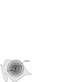
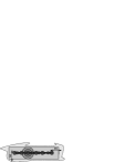
Figure 6: Geometry of the parameters underlying a) representation $\pi$ and b) representations $\alpha,\tilde{\beta},\tilde{\gamma}$.

Lemma 3.2

1. Let $r>1$. Then it holds $t\leq C\cdot r^{t}$ for all $t>0$, where $C:=1/(e\cdot\ln r)$.

2. More generally, $t^{s}\leq(\tfrac{s}{e\ln r})^{s}\cdot r^{t}$ for all $t>0$ and $s\geq 0$ with the convention of $0^{0}=1$.

3. For all $N\in\mathbb{N}$ it holds $1+\tfrac{\ln 2}{N}\leq\sqrt[N]{2}\leq 1+\tfrac{1}{N}$.

4. Asymptotically $1/\ln(r)=\Theta(\tfrac{1}{r-1})$ as $r\searrow 1$.

5. With $\bar{a}\in C^{\omega}_{1}$ and $(K,A)$ as in Definition 3.1, for every $|z|\leq r^{\prime}:=\sqrt[2K]{2}=\sqrt{r}$ it holds $|f_{\bar{a}}(z)|\leq A\cdot\tfrac{r^{\prime}}{r^{\prime}-1}$ and $|f_{\bar{a}}^{(d)}(z)|\leq A\cdot d!/(r^{\prime}-1)^{d+1}$, $d\in\mathbb{N}$.

6. For all $k\geq 2$ and $x\geq k^{2}$ it holds $x^{k}\leq\exp(x)$.
   For all $a,k\geq 1$ and $b>0$ and $x\geq k^{2}\cdot a^{1/k}/b^{2}\geq 4$ it holds $a\cdot x^{k}\leq\exp(x\cdot b)$.

Proof

Any local extreme point point $x_{0}$ of $0<x\mapsto x\cdot r^{-x}$ is a root of $\tfrac{d}{dx}x\cdot r^{-x}=r^{-x}-\ln(r)\cdot x\cdot r^{-x}$, i.e. $t\cdot r^{-t}\leq C:=\max\{x\cdot r^{-x}:x>0\}$ attained at $x_{0}:=1/\ln(r)$. Replacing $r$ with $r^{1/s}$ yields b). For c) observe $\sqrt[N]{2}=\exp(\ln 2/N)$ and analyze $\exp(x)$ on $[0;\ln 2]\ni x:=1/N$. Taylor expansion yields $\ln(1-x)\approx-\tfrac{1}{x}-\tfrac{1}{2x^{2}}-\cdots$ for $x:=1-r$.
Regarding e), $|f_{\bar{a}}(z)|\leq\sum_{j}|a_{j}|\cdot|z|^{j}\leq A\cdot\sum_{j}(r^{\prime}/r)^{j}A\tfrac{1}{1-r^{\prime}/r}=A\cdot\tfrac{r^{\prime}}{r^{\prime}-1}$ and $|f^{(d)}(z)|\leq A\cdot\sum_{j\geq d}j\cdot(j-1)\cdots(j-d+1)(|z|/r^{\prime})^{j-d}=A\tfrac{d^{d}}{dt^{d}}\sum_{j}q^{j}\big{|}_{q=|z|/r^{\prime}}\leq A\tfrac{d^{d}}{dq^{d}}\tfrac{1}{1-q}\big{|}_{q=|z|/r^{\prime}\leq r^{\prime}}\leq A\cdot d!/(r^{\prime}-1)^{d+1}$.
Turning to f), first record that $k^{2}\leq\exp(k)$ holds for all $k\geq 2$. In particular $x\leq\exp(x/k)$ is true for $x=k^{2}$; and monotone in $x$ because of $\partial_{x}x=1\leq 1/k\exp(x/k)=\partial_{x}\exp(x/k)$ for all $x\geq k^{2}$.
Concerning the second claim substitute $y:=x\cdot a^{1/k}$ and conclude from the first that $y^{k\cdot a^{1/k}/b}\leq\exp(y)$ for all $y\geq k^{2}\cdot a^{2/k}/b^{2}\geq 4$. ∎

Theorem 3.3

1. Evaluation  $C^{\omega}\!\left(\overline{\operatorname{ball}}(0,1)\right)\times\overline{\operatorname{ball}}(0,1)\ni(f,z)\mapsto f(z)\in\mathbb{C}$  is fully polytime $(\pi\times\rho_{\text{\rm dy}}^{2},\rho_{\text{\rm dy}}^{2})$–computable, that is within time polynomial in $n+K+\log A$ for the parameters $(K,A)$ according to Definition 3.1.

2. Addition  $C^{\omega}\!\left(\overline{\operatorname{ball}}(0,1)\right)\times C^{\omega}\!\left(\overline{\operatorname{ball}}(0,1)\right)\ni(f_{1},f_{2})\mapsto f_{1}+f_{2}\in C^{\omega}\!\left(\overline{\operatorname{ball}}(0,1)\right)$  is fully polytime $(\pi\times\pi,\pi)$–computable, that is within time polynomial in $n+K_{1}+K_{2}+\log A_{1}+\log A_{2}$.

3. Multiplication  $C^{\omega}\!\left(\overline{\operatorname{ball}}(0,1)\right)\times C^{\omega}\!\left(\overline{\operatorname{ball}}(0,1)\right)\ni(f_{1},f_{2})\mapsto f_{1}\cdot f_{2}\in C^{\omega}\!\left(\overline{\operatorname{ball}}(0,1)\right)$  is fully polytime $(\pi\times\pi,\pi)$–computable.

4. Differentiation  $C^{\omega}\!\left(\overline{\operatorname{ball}}(0,1)\right)\ni f\mapsto f^{\prime}\in C^{\omega}\!\left(\overline{\operatorname{ball}}(0,1)\right)$  is fully polytime $(\pi,\pi)$–computable.
   More generally $d$-fold differentiation  $C^{\omega}\!\left(\overline{\operatorname{ball}}(0,1)\right)\times\mathbb{N}\ni(f,d)\mapsto f^{(d)}\in C^{\omega}\!\left(\overline{\operatorname{ball}}(0,1)\right)$  is fully polytime $\big{(}\pi+\operatorname{unary}(d),\pi\big{)}$–computable, that is within time polynomial in $n+K+\log A+d$.

5. Anti-differentiation  $C^{\omega}\!\left(\overline{\operatorname{ball}}(0,1)\right)\ni f\mapsto\int f=F\in C^{\omega}\!\left(\overline{\operatorname{ball}}(0,1)\right)$  is fully polytime $(\pi,\pi)$–computable; and $d$-fold anti-differentiation is fully polytime $\big{(}\pi+\operatorname{unary}(d),\pi\big{)}$–computable.

6. Parametric maximization, that is both the mappings $\operatorname{MAX}\circ\operatorname{Re}$ and $|\operatorname{MAX}|$ from $C^{\omega}\!\left(\overline{\operatorname{ball}}(0,1)\right)\times[-1;1]^{2}$ to $\mathbb{R}$ are fully polytime $(\pi\times\rho_{\text{\rm dy}}^{2},\rho_{\text{\rm dy}})$–computable, where

   $$\operatorname{MAX}\circ\operatorname{Re} :(f,u,v)\;\mapsto\;\max\big{\{}\operatorname{Re}f(x):\min(u,v)\leq x\leq\max(u,v)\big{\}}\quad\text{ and }\quad$$

   $$|\operatorname{MAX}| :(f,u,v)\;\mapsto\;\max\big{\{}|f(x)|:\min(u,v)\leq x\leq\max(u,v)\big{\}}\enspace.$$

7. As a converse to a), given a $\rho_{\text{\rm dy}}^{\mathbb{D}}$–name of $f$ as well as $K\in\mathbb{N}$ and an integer upper bound $B$ on $\max\big{\{}|f(z)|:|z|\leq\sqrt[K]{2}\big{\}}$ and $j\in\mathbb{N}$, the coefficient $a_{j}=f^{(j)}(0)/j!$ is computable within time polynomial in $n+K+\log B+j$; formally: the partial function

   $$C^{\omega}\!\left([-1;1]\right)\times\mathbb{N}\times\mathbb{N}\;\ni\;(f,K,B)\;\mapsto\bar{a}:\quad f=f_{\bar{a}},\;\forall|z|\leq\sqrt[K]{2}:|f(z)|\leq B$$

   is polytime $\big{(}\rho_{\text{\rm dy}}^{\mathbb{D}}+\operatorname{binary}\langle 2^{K},B\rangle,\rho_{\text{\rm dy}}^{\omega}\big{)}$–computable.

Note that, for real-valued $f$, $\min\{f(z):z\}=-\max\{-f(z):z\}$ and $\max\{|f(z)|:z\}=\max\big{(}\max\{f(z):z\},-\min\{f(z):z\}\big{)}$. Hence the above Items a) to f) indeed constitute a natural choice of basic primitive operations on $C^{\omega}\!\left(\overline{\operatorname{ball}}(0,1)\right)$.

Proof (Theorem 3.3)

1. Given $K$, calculate $r:=\sqrt[K]{2}$ within time polynomial in $n+K$. Then evaluate the first roughly $N:=n\cdot K+\log A$ terms of the power series on the given $z$: according to Equation (10) the tail $\sum_{j\geq N}|a_{j}|\cdot|z|^{j}\leq A\cdot\sum_{j\geq N}(|z|/r)^{j}=A\cdot(|z|/r)^{N}\tfrac{1}{1-|z|/r}$ is then small of order $(|z|/r)^{n\cdot K}=\mathcal{O}(2^{-n})$ because of $|z|\leq 1$.

2. Given $(\bar{a},K,A)$ and $(\bar{b},L,B)$ output $(\bar{c},M,C)$ where $c_{j}:=a_{j}+b_{j}$ and $C:=A+B$ and $M:=\max(K,L)$. In view of Example 1.7b), approximating $c_{j}$ up to error $2^{-m}$ this is possible in time polynomial in $m+\log(A+B)+j\cdot(K+L)$; now recall Definition 1.9e)

3. Similarly, given $(\bar{a},K,A)$ and $(\bar{b},L,B)$ output $(\bar{c},M,C)$ where $c_{j}:=\sum_{i=0}^{j}a_{i}\cdot b_{j-i}$ and $C$ is some integer $\geq A\cdot B\cdot\big{(}1+M/(e\cdot\ln 2)\big{)}$ where $M:=2\max(K,L)$. Indeed, with $r_{A}\geq(2)^{\tfrac{1}{K}}$ and $r_{B}\geq(2)^{\tfrac{1}{L}}$ and $r=\min(r_{A},r_{B})\geq(2)^{\tfrac{2}{M}}$, $1<r^{\prime}:=(2)^{\tfrac{1}{M}}\leq\sqrt{r}<r$ implies $j\leq\sqrt{r^{j}}/(e\cdot\ln\sqrt{r})\leq M\cdot\sqrt{r}^{j}/(e\cdot\ln 2)$ according to Lemma 3.2a); hence $|c_{j}|\leq\sum_{i=0}^{j}A/r_{A}^{i}\cdot B/r_{B}^{j-i}=A\cdot B\cdot(j+1)/r^{j}\leq C/\sqrt{r}^{j}$.

4. Given $(\bar{,}K,A)$ output $(\bar{a}^{\prime},K^{\prime},A^{\prime})$ with $(a_{j}^{\prime}):=\big{(}(j+1)\cdot a_{j+1}\big{)}$ and $K^{\prime}:=2K$ and $A^{\prime}$ some integer $\geq\tfrac{A}{r}\cdot(1+\tfrac{2K}{e\ln 2})$. Indeed, $1<r^{\prime}:=(2)^{\tfrac{1}{K^{\prime}}}=\sqrt{r}<r$ implies $j\leq 2K\cdot\sqrt{r}^{j}/(e\ln 2)$ according to Lemma 3.2a); hence $(j+1)\cdot|a_{j+1}|\leq A^{\prime}/\sqrt{r}^{j}$.
   More generally, in view of Lemma 3.2b), output $\big{(}(j+1)\cdot(j+2)\cdots(j+d)\cdot a_{j+d}\big{)}_{{}_{j}}$ and $K^{\prime}:=2K$ and $A^{\prime}\geq\tfrac{A}{r^{d}}\cdot d^{d}\cdot(1+2K)^{d}\geq\tfrac{A}{r^{d}}\cdot(1+\tfrac{2Kd}{e\ln 2})\cdot(2+\tfrac{2Kd}{e\ln 2})\cdots(d+\tfrac{2Kd}{e\ln 2})$.

5. Given $(\bar{a},K,A)$, in case $d=1$ output $a_{0}^{\prime}:=0$ and $a_{j}^{\prime}:=a_{j-1}/j$ and $K^{\prime}:=K$ and $A^{\prime}\geq A\cdot r$. In the general case $a_{j}^{\prime}=a_{j-d}/j/(j-1)/\cdots/(j-d+1)$ and $A^{\prime}\geq A\cdot r^{d}$.

6. First suppose that $f|_{[-1;1]}$ is real, i.e. $a_{j}\in\mathbb{R}$. Similar to a), the first $d:=\mathcal{O}(n\cdot K+\log A)$ terms of the series yield a polynomial $p\in\mathbb{D}_{n+1}[X]$ of $\deg(p)<d$ with dyadic coefficients uniformly approximating $f$ up to error $2^{-n-1}$. In particular it suffices to approximate the maximum of $p$ on $[u^{\prime},v^{\prime}]$ up to $2^{-n-1}$ (for $u^{\prime},v^{\prime}\in\mathbb{D}$ sufficiently close to $u$ and $v$, respectively). This can be achieved by bisection on $y$ w.r.t. the following existentially quantified formula in the first-order equational theory of the reals with dyadic parameters which, involving only a constant number of polynomials and quantifiers, can be decided in time polynomial in the degree and binary coefficient length [BPR06, Exercise 11.7]:

   $$\Phi(u^{\prime},v^{\prime},p_{0},\ldots,p_{d-1})\;\;:=\;\;``\exists x,r,s,t\in\mathbb{R}:\;\;\underbrace{x=u^{\prime}+r^{2}}_{\geq u^{\prime}}\;\wedge\;\underbrace{v^{\prime}=x+s^{2}}_{x\leq v^{\prime}}\;\wedge\;\underbrace{p(x)=y+t^{2}}_{p(x)\geq y}"$$

   In the general case of a complex valued $f|_{[-1;1]}$, $|f|^{2}=\operatorname{Re}(f)^{2}+\operatorname{Im}(f)^{2}$ is uniformly approximated by the real polynomial $q:=\operatorname{Re}(p)^{2}+\operatorname{Im}(p)^{2}$, thus $\max|f|^{2}$ is polytime computable as above. Since both $\mathbb{R}\ni t\mapsto t^{2}$ and $\mathbb{R}_{+}\ni s\mapsto\sqrt{s}$ are monotonic and polytime computable, the same follows for $\max|f|=\sqrt{\max|f|^{2}}$.

7. According to Cauchy’s differentiation formula (9), Equation (10) is satisfied with $A:=B$. Polytime computability of the sequence $a_{j}=f^{(j)}(0)/j!$ from evaluations of $f|_{[-1;1]}$ is due [Müll87]; cmp. also the proof of [Ko91, Theorem 6.9] and (that of) Theorem 4.6a) below. and note that both $\operatorname{Re}f$ and $\operatorname{Im}f$ are real analytic. Since $|f^{\prime}(x)|\leq A/(r^{\prime}-1)^{2}\leq A\cdot(\tfrac{2K}{\ln 2})^{2}$ according to a) and Lemma 3.2c), we known that $\mu(n)=n+\lceil\log A+2\log\tfrac{2K}{\ln 2}\rceil$ is a modulus of continuity of $f|_{[-1;1]}$ and can suffice with evaluations on the dense subset $[-1;1]\cap\mathbb{D}$. ∎

3.2 Representing, and Operating on, Analytic Functions on $[0;1]$

We now consider functions $f\in C^{\omega}[0;1]$, that is functions analytic on some complex neighbourhood of $[0;1]$. Being members of $\operatorname{Lip}[0;1]$, the second-order representation $\rho_{\text{\rm dy}}^{\mathbb{D}}+\operatorname{binary}(\operatorname{Lip})$ applies. On the other hand, $f$ is covered by finitely many power series, each naturally encoded via $\pi$. And Equation 2 suggests yet yet another encoding:

Definition 3.4

Let $C^{\omega}\!\left([0;1]\right)$ denote the space of complex-valued functions analytic on some complex neighbourhood of $[0;1]$.

1. Let $M\in\mathbb{N}$ and $x_{m}\in[0;1]$ and $a_{m,j}\in\mathbb{C}$ and $L_{m}\in\mathbb{N}$ and $A_{m}\in\mathbb{N}$ ($1\leq m\leq M$, $j\in\mathbb{N}$).
   We say that $\big{(}M,(x_{m}),(a_{m,j}),(L_{m}),(A_{m})\big{)}$ represents $f\in C^{\omega}\!\left([0;1]\right)$ if it holds

   $$[0;1]\subseteq\bigcup\limits_{m=1}^{M}\big{[}x_{m}-\tfrac{1}{4L_{m}},x_{m}+\tfrac{1}{4L_{m}}\big{]}\;\;\text{and}\;\;f^{(j)}(x_{m})=a_{m,j}\cdot j!\;\;\text{and}\;\;|a_{m,j}|\leq A_{m}\cdot L_{m}^{j}$$ (11)

   An $\alpha$–name of $f$ encodes ($M$ in unary and, jointly in the sense Remark 1.8c) for each $1\leq m\leq M$ the following: a $\rho_{\text{\rm dy}}$–name of $x_{m}$, a $(\rho_{\text{\rm dy}}^{2})^{\omega}$–name of $(a_{m,j})_{{}_{j}}$ as well as advice $A_{m}$ in binary and $L_{m}$ in unary with parameter $\langle\log A_{1},{L_{1}},\log A_{2},{L_{2}},\ldots,\log A_{m},{L_{m}}\rangle$.

2. Define second-order representation $\tilde{\beta}$ to encode $f$ via (see Figure 6b)

   • a $\rho_{\text{\rm dy}}^{\mathbb{D}}$–name of $\operatorname{Re}f|_{[0;1]}$

   • and one of $\operatorname{Im}f|_{[0;1]}$, together with

   • an integer $L$ in unary such that $f\in C^{\omega}\!\left(\overline{\mathcal{R}}_{L}\right)$,
     where $\overline{\mathcal{R}}_{L}:=\{x+iy\mid-\tfrac{1}{L}\leq y\leq\tfrac{1}{L},-\tfrac{1}{L}\leq x\leq 1+\tfrac{1}{L}\}$

   • and a binary integer upper bound $B$ to $|f|$ on said $\overline{\mathcal{R}}_{L}$.

3. A $\tilde{\gamma}$–name of $f\in C^{\omega}\!\left([0;1]\right)$ consists of a $\rho_{\text{\rm dy}}^{\mathbb{D}}$–name of $\operatorname{Re}f|_{[0;1]}$ and one of $\operatorname{Im}f|_{[0;1]}$ enriched with advice parameters $A$ (in binary) and $K$ (in unary) such that $|f^{(j)}(x)|\leq A\cdot K^{j}\cdot j!$ holds for all $0\leq x\leq 1$.

Again, the binary and unary encodings have been chosen carefully: Analogous to $K$ in Definition 3.1 upper bounding $1/(R-1)$, the distance of the domain $\overline{\operatorname{ball}}(0,1)$ to a singularity, here $1/L$ constitutes a lower bound on the distance of $[0;1]$ to any complex singularity of $f$. Specifically the size of a $\tilde{\beta}$–name $\psi$ of $f$ is $|\psi|(n)=\Theta(n+L+\log B)$; and that of a $\tilde{\gamma}$–name is $\Theta(n+K+\log A)$.

Example 3.5

1. For $x_{m}\in[0;1]$ and $y_{m}>0$ ($1\leq m\leq M$) the function $z\mapsto\prod_{m}\big{(}(z-x_{m})^{2}+y_{m}^{2}\big{)}^{-1}$ is analytic on $[0;1]$ with complex singularities at $x_{m}\pm iy_{m}$.

2. The Gaussian function $g_{1}(x)=\exp(-x^{2})$ employed in the proof of Example 2.6f) has $g_{1}^{(j)}(x)=(-1)^{j}\cdot H_{j}(x)\cdot g_{1}(x)$ with the Hermite Polynomials

   $$H_{0}=1,\quad H_{1}(x)=2x,\quad H_{n+1}(x)=2x\cdot H_{n}(x)-2n\cdot H_{n-1}(x)\enspace.$$

   A simple uniform bound on $g_{1}^{(j)}$ is obtained using Equation (9):

   $$|g_{1}^{(j)}(x)|\;\leq\;\tfrac{j!}{2\pi}\cdot\int\nolimits_{|z-x|=1}|\exp(-z^{2})|/1^{j}\,dz\;\leq\;j!e$$

   because $|\exp(-z^{2})|=\exp\big{(}-\operatorname{Re}^{2}(z)+\operatorname{Im}^{2}(z)\big{)}\leq\exp(1)$ due to $|z-x|=1$ with $x\in\mathbb{R}$.

Hence in both cases, $f|_{[0;1]}$ being large/steep or a complex singularity residing close-by, more time is (both needed and) granted for polytime calculations on $f$. Similarly for the parameterized representation $\alpha$. Also note that a $\tilde{\gamma}$–name of $f$ encodes only data on the restriction $f|_{[0;1]}$ whereas both $\alpha$ and $\tilde{\beta}$ explicitly refer to the complex differentiable $f$ with open domain; cmp. [KrPa02].

Remark 3.6

1. Both $\tilde{\beta}$ and $\tilde{\gamma}$ enrich $\rho_{\text{\rm dy}}^{\mathbb{D}}$–names with different discrete information (and thus without affecting the nonuniform complexity where $n$ is considered the only parameter) of the kind commonly omitted in nonuniform claims and are thus candidates for uniformly refining Example 1.6.

2. We could (and in Section 4 will) combine in the definition of $\tilde{\gamma}$ the binary $A$ with unary $K$ into one single binary $C:=A\cdot 2^{K}$ satisfying $\|f^{(j)}\|\leq C\cdot(\log C)^{j}\cdot j!$

Theorem 3.7

1. On $C^{\omega}\!\left([0;1]\right)$, $\alpha$ and $\tilde{\beta}$ and $\tilde{\gamma}$ constitute mutually (fully) polytime-equivalent (parameterized) representations.

2. The following operations from Theorem 3.3 are in fact uniformly polytime computable on $C^{\omega}\!\left([0;1]\right)$:
   Evaluation (i), addition (ii), multiplication (iii), iterated differentiation $(\textup{{1}}^{d},f)\mapsto f^{(d)}$ (iv), parametric integration (v), and parametric maximization (vi).

3. Composition (vii), that is the partial operator

   $$(g,f)\mapsto g\circ f\quad\text{ for }\quad f,g\in C^{\omega}\!\left([0;1]\right)\quad\text{ with }\quad f\big{|}_{[0;1]}\in C^{\omega}\!\left([0;1],[0;1]\right)\enspace,$$

   is fixed-parameter computable in the sense of Definition 2.4h). More precisely in terms of $(\tilde{\beta}\times\tilde{\beta},\tilde{\beta})$–computability, given integers $A,K$ with $|f(z)|\leq A$ on $\overline{\mathcal{R}}_{K}$ and $(L,B)$ with $|g(z)|\leq B$ on $\overline{\mathcal{R}}_{L}$, $g\circ f$ is analytic on $\overline{\mathcal{R}}_{2AKL}$ and thereon bounded (like $g$ itself) by $B$. Note that (only) the unary length of $2AKL$ is exponential in (only) the binary length of $A$.
   Similarly concerning $(\tilde{\gamma}\times\tilde{\gamma},\tilde{\gamma})$–computability, $f$ with advice parameters $(A,K)$ and $g$ with advice parameters $(B,L)$ gets mapped to $g\circ f$ with advice parameters $\big{(}\tfrac{A\cdot B\cdot L}{1+A\cdot L},K\cdot(1+A\cdot L)\big{)}$, where the unary length of (only) the latter is exponential in (only) the binary length of $A$.

Recall that, since both $\tilde{\beta}$–names and $\tilde{\gamma}$–names have length $\mathcal{O}(n+k)$ linear in $n$ with constant parameter $k$, second-order polynomials here boil down to ordinary polynomials in $n+k$ (Observation 1.18a+b+c).

Proof (Theorem 3.7)

a)

Since $f$ is complex analytic on some $U\supseteq[0;1]$ open in $\mathbb{C}$ there exists an $L\in\mathbb{N}$ as required for a $\tilde{\beta}$–name. The continuous $|f|$ is bounded on compact $\overline{\mathcal{R}}_{L}$ by some $B$.

$\tilde{\beta}\preceq_{\text{\rm P}}^{2}\tilde{\gamma}$:

The $\rho_{\text{\rm dy}}^{\mathbb{D}}$–names as part of the desired $\tilde{\gamma}$–name are already contained in the $\tilde{\beta}$–name. Now observe that Cauchy’s differentiation formula (9) implies $|f^{(j)}(x)|/j!\leq B\cdot L^{j}$ for all $j\in\mathbb{N}$ and all $x\in[0;1]$. Hence $A:=B$ and $K:=L$ are suitable choices.

$\tilde{\gamma}\preceq_{\text{\rm P}}^{2}\alpha$:

Given $A,K$ set $L_{m}:=K$ and $A_{m}:=A$ and $M:=4K+1$ and $x_{m}:=(m-1)/(4K)$, noting that $(M,L_{1},\ldots,L_{M},A_{1},\ldots,A_{M},x_{1},\ldots,x_{M})$ can be computed within second-order polytime: with $A_{m}$ encoded in binary and $L_{m}$ unary, the output has length $\mathcal{O}\big{(}M\cdot(K+\log A)\big{)}$ compared to the unary encoding length $\Omega(K+\log A)$ of the input. We claim that also the sequences $a_{m,j}=f^{(j)}(x_{m})/j!$ can be obtained within time a second-order polynomial in the size of the given $\tilde{\gamma}$–name. In order to apply Theorem 3.3g) observe that, since $|a_{m,j}|\leq A\cdot K^{j}$, the translated and scaled function $\hat{f}_{m}(z):=f\big{(}x_{m}+\tfrac{z}{2K}\big{)}$ can be evaluated efficiently on $\mathbb{D}$ using the $\tilde{\varphi}$–name of $f$; and is analytic on $\operatorname{ball}(0,2)$ with Taylor coefficients $\hat{a}_{m,j}:=\hat{f}_{m}^{(j)}(0)/j!=f^{(j)}(x_{m})/(2K)^{j}/j!$ bounded by $A/2^{j}$. Hence $\big{(}(\hat{a}_{m,j})_{{}_{j}},(\hat{K}:=1),A\big{)}$ constitutes an $\alpha$–name of $\hat{f}_{m}$; from which $a_{m,j}=\hat{a}_{m,j}\cdot(2K)^{j}$ can be recovered.

$\alpha\preceq_{\text{\rm p}}\tilde{\beta}$:

Let $\big{(}M,(x_{m}),(a_{m,j}),(L_{m}),(A_{m})\big{)}$ denote an $\alpha$–name of $f$. From $|a_{m,j}|\leq A_{m}\cdot L_{m}^{j}$ observe that $f$ is analytic on $\bigcup_{m}\operatorname{ball}(x_{m},\tfrac{1}{L_{m}})$; which constitutes an open neighbourhood of $\overline{\mathcal{R}}_{L}$ for $L:=2\cdot\max_{m}L_{m}$ because of $[0;1]\subseteq\bigcup_{m=1}^{M}\big{[}x_{m}-\tfrac{1}{4L_{m}},x_{m}+\tfrac{1}{4L_{m}}\big{]}$; and $f$ is bounded on $\overline{\mathcal{R}}_{L}$ by $\max\big{\{}|\sum_{j}a_{m,j}(z-x_{m})^{j}|:m\leq M,z\in\operatorname{ball}(x_{m},\tfrac{1}{4L_{m}}\big{\}}\leq\max_{m}\sum_{j}A_{m}L_{m}^{j}\cdot\tfrac{1}{4L_{m}}^{j}=\tfrac{4}{3}\max_{m}A_{m}$. Both $L$ and $B\geq\tfrac{4}{3}\max_{m}A_{m}$ can easily be calculated in time polynomial in the parameter $k=\Theta\big{(}\sum_{m}(L_{m}+\log A_{m})\big{)}$. It thus remains to prove $\alpha\preceq_{\text{\rm p}}\rho_{\text{\rm dy}}^{\mathbb{D}}$ as follows:
Given $x\in[0;1]$, some (of at least two) $m$ with $x\in J_{m}:=\big{[}x_{m}-\tfrac{1}{2L_{m}},x_{m}+\tfrac{1}{2L_{m}}\big{]}$ can be found within time polynomial in $\sum_{m}\log L_{m}$: due to the factor-two overlap, it suffices to know $x$ up to error $\tfrac{1}{4L_{m}}$. Finally observe that $\hat{f}_{m}(z):=f\big{(}x_{m}+\tfrac{z}{2L_{m}}\big{)}$ is analytic on $\operatorname{ball}(0,2)$ with coefficients $\hat{a}_{m,j}=f_{m}^{(j)}(0)/j!=a_{m,j}/(2L_{m})^{j}$ satisfying $|\hat{a}_{m,j}|\leq A_{m}/2^{j}$; hence can be evaluated on $\overline{\operatorname{ball}}(0,1)$ by Theorem 3.3a) within time polynomial in $K+\log A_{m}+n$ for $K:=1$. This provides for the evaluation within time polynomial in $n$ and $k$ of $J_{m}\ni x\mapsto\hat{f}_{m}\big{(}(x-x_{m})\cdot 2L_{m}\big{)}=f(x)$, i.e. of $f|_{[0;1]}$.

b)

Note that in view of a) we may freely choose among representations $\alpha,\tilde{\beta},\tilde{\gamma}$ output and even any combination of them for input.

i)

Evaluation is provided by the $\rho_{\text{\rm dy}}^{\mathbb{D}}$–information contained in a $\tilde{\gamma}$–name of $f$ together with the Lipschitz bound $|f^{\prime}(x)|\leq AK$ of binary length polynomial in $k=\Theta(K+\log A)$.

ii)

Given $\rho_{\text{\rm dy}}^{\mathbb{D}}$–names of $f_{1},f_{2}$ and $L_{1},L_{2}$ in unary and binary $B_{1},B_{2}$ according to $\tilde{\beta}$, output a $\rho_{\text{\rm dy}}^{\mathbb{D}}$–name of $f:=f_{1}+f_{2}$ (Example 2.6a) and $L:=\max(L_{1},L_{2})$ and $B=B_{1}+B_{2}$.

iii)

Similarly with $f:=f_{1}\cdot f_{2}$ and $L:=\max(L_{1},L_{2})$ and $B:=B_{1}\cdot B_{2}$.

iv)

Given an $\alpha$–name $\big{(}M,(x_{m}),(a_{m,j}),(L_{m}),(A_{m})\big{)}$ of $f$ and in case $d=1$, (the proof of) Theorem 3.3d) yields $A_{m}^{\prime}$ such that the coefficients $\hat{a}^{\prime}_{m,j}=(j+1)\cdot\hat{a}_{m,j+1}=(j+1)\cdot a_{m,j+1}/(2L_{m})^{j+1}$ of $\hat{f}^{\prime}_{m}(z)=\tfrac{d}{dz}f\big{(}x_{m}+\tfrac{z}{2L_{m}}\big{)}$ satisfy $|\hat{a}^{\prime}_{m,j}|\leq A_{m}^{\prime}/\sqrt{2}^{j}$. Note that the bounds $|a^{\prime}_{m,j}|\leq A_{m}^{\prime}\cdot L^{\prime j}_{m}$ on $a^{\prime}_{m,j}=\hat{a}^{\prime}_{m,j}\cdot(2L_{m})^{j}$ thus obtained apply to $L^{\prime}_{m}=\sqrt{2}L_{m}$ and hence may fail the covering property of Equation (11). Nevertheless they do support efficient evaluation of $\hat{f}^{\prime}_{m}$ on $\overline{\operatorname{ball}}(0,1)$ by Theorem 3.3a), but now with $K:=2$. Given $x\in[0;1]$, similarly to the above proof of “$\alpha\preceq_{\text{\rm p}}\tilde{\beta}$” some $J_{m}$ containing $x$ can be found efficiently and used to calculate $f^{\prime}(x)=\hat{f}^{\prime}_{m}\big{(}(x-x_{m})\cdot 2L_{m}\big{)}\cdot 2L_{m}$. This provides for a $\rho_{\text{\rm dy}}^{\mathbb{D}}$–name of $f^{\prime}$; as part of a $\tilde{\gamma}$–name to output. And for given $(K,A)$ satisfying $|f^{(j)}(x)|\leq A\cdot K^{j}\cdot j!$, Lemma 3.2a) implies $|(f^{\prime})^{(j)}(x)|=|f^{(j+1)}(x)|\leq AK\cdot(j+1)\cdot K^{j}\cdot j!\leq AK\cdot(2K)^{j}\cdot j!$ since $\tfrac{1}{e\ln 2}\leq 1$; hence $(AK,2K)$ yields the rest of a $\tilde{\gamma}$–output. In case $d>1$, similarly, $|f^{(d+j)}(x)|\leq AK^{d}\cdot(j+1)\cdots(j+d)\cdot K^{j}\cdot j!\leq A\cdot(dK)^{d}\cdot(2K)^{j}\cdot j!$ according to Lemma 3.2b); hence output $\big{(}A\cdot(dK)^{d},2K\big{)}$ of binary length polynomial in $d$ (sic!) and $K+\log A$.

vi)

Given $0\leq u\leq v\leq 1$ and an $\alpha$–name $\big{(}M,(x_{m}),(a_{m,j}),(L_{m}),(A_{m})\big{)}$ of $f$, the idea is to partition $[u;v]$ into $K\leq\mathcal{O}(m)$ sub-intervals $I_{k}=[u_{k};v_{k}]$ each lying completely within some $J_{m}$ and then apply Theorem 3.3f) to $\hat{f}_{m}(z):=f\big{(}x_{m}+\tfrac{z}{2L_{m}}\big{)}$ in order to obtain $y_{k}:=\max\{f(x):x\in I_{k}\}$ and finally $\max\{f(x):u\leq x\leq v\}=\max\{y_{k}:k\leq K\}$.
It follows from the proof of $\tilde{\gamma}\preceq_{\text{\rm P}}^{2}\alpha$ that we may w.l.o.g. suppose $L_{m}\equiv L$ and $(x_{m})$ increasing with equidistance $\leq\tfrac{1}{4L}$. So find some $1\leq m\leq m^{\prime}\leq M$ with $u\in J_{m}$ and $v\in J_{m^{\prime}}$. Then $u_{1}:=u$ and $v_{1}:=\min\big{(}v,x_{m}+\tfrac{1}{2L}\big{)}$ yield the first interval; the next are given by $u_{k+1}:=v_{k}$ and $v_{k+1}:=x_{m+k}+\tfrac{1}{2L}\geq u_{k+1}$ ($1\leq k\leq m^{\prime}-m-1$); and the last by $u_{m^{\prime}-m}:=v_{m^{\prime}-m-1}$ and $v_{m^{\prime}-m}:=\max\big{(}u,x_{m^{\prime}}-\tfrac{1}{2L}\big{)}$.

v)

Similarly to vi) but now with $y_{k}=\int_{u_{k}}^{v_{k}}f(x)\,dx=F(v_{k})-F(u_{k})$ a local anti-derivative of $f$ according to Theorem 3.3e) and $\int_{u}^{v}f(x)\,dx=\sum_{k}y_{k}$.

vii)

Looking at $(\tilde{\beta}\times\tilde{\beta},\tilde{\beta})$–computability, in view of Example 2.6b) it remains to obtain, given integers $(L,B)$ with $|g(z)|\leq B$ on $\overline{\mathcal{R}}_{L}$ and $A,K$ with $|f(z)|\leq A$ on $\overline{\mathcal{R}}_{K}$, similar quantities for $g\circ f$. To this end employ Cauchy’s differentiation formula (9) to deduce $|f^{\prime}(z)|\leq A\cdot(2K)$ on $\overline{\mathcal{R}}_{2K}$. Now the Mean Value Theorem (in $\operatorname{Re}z$ and $\operatorname{Im}z$ considered as two real variables!) implies $|f(x)-f(x+z)|\leq 2AK\cdot|z|\leq 1/L$ for $x\in[0;1]$ and $z\in\overline{\mathcal{R}}_{2AKL}$. Together with the hypothesis of $f$ mapping $[0;1]$ to $[0;1]$, this shows $f$ to map $\overline{\mathcal{R}}_{2AKL}$ to $\overline{\mathcal{R}}_{L}\subseteq\operatorname{dom}(g)$. Therefore $g\circ f$ is analytic on some open neighbourhood of $\overline{\mathcal{R}}_{2AKL}$ and thereon bounded (like $g$ itself) by $B$.
Concerning $(\tilde{\gamma}\times\tilde{\gamma},\tilde{\gamma})$–computability, the proof of [KrPa02, Proposition 1.4.2] using the formula of Faá di Bruno (cmp. below Fact 4.4f) shows that $|f^{(j)}|\leq A\cdot K^{j}\cdot j!$ and $|g^{(j)}|\leq B\cdot L^{j}\cdot j!$ imply $|(g\circ f)^{(j)}|\leq C\cdot M^{j}\cdot j!$ where $C:=\frac{A\cdot B\cdot L}{1+A\cdot L}$ and $M:=K\cdot(1+A\cdot L)$. ∎

3.3 Representing, and Operating on, Entire Functions

As has been kindly pointed out by Torben Hagerup, the above Theorems 3.3 and 3.7 both do not capture the important case of the exponential function on entire $\mathbb{R}$ (Example 2.3a) or $\mathbb{C}$.

Definition 3.8

On the space $C^{\omega}_{\infty}=\big{\{}\bar{a}\subseteq\mathbb{C},R(\bar{a})=\infty\big{\}}$, a $\tilde{\varepsilon}$–name $\psi$ of $\bar{a}=(a_{j})_{{}_{j}}\in C^{\omega}_{\infty}$ is a mapping $\psi:\{0,1\}^{*}\to\{0,1\}^{*}$ of the form

$$\textup{{1}}^{n}\;\mapsto\;\sigma_{n}\,\operatorname{bin}\big{(}B(n)\big{)}$$

where $\bar{\sigma}$ is a $(\rho_{\text{\rm dy}}^{2})^{\omega}$–name of $\bar{a}$ and $B:\mathbb{N}\to\mathbb{N}$ a function satisfying

$$\forall M\in\mathbb{N}\;\forall j\in\mathbb{N}:\quad|a_{j}|\;\leq\;B(M)/M^{j}\enspace.$$ (12)

Note that this second-order representation has names of super-linear length, that is, employing the full power of second-order size parameters. Indeed, every mapping $B:\mathbb{N}\to\mathbb{N}$ gives rise to an entire function with Taylor coefficients $a_{j}:=\inf_{M}B(M)/M^{j}$.

Theorem 3.9

1. $\tilde{\varepsilon}$ is a second-order representation, and it holds $\tilde{\varepsilon}\big{|}^{C^{\omega}_{1}}\preceq_{\text{\rm P}}^{2}\pi$

2. Evaluation

   $$C^{\omega}_{\infty}\times\mathbb{C}\;\ni\;(\bar{a},z)\;\mapsto\;\sum\nolimits_{j}a_{j}z^{j}\;\in\;\mathbb{C}$$

   is $\big{(}\tilde{\varepsilon},(\rho_{\text{\rm dy}}^{2},|\rho_{\text{\rm dy}}^{2}|),\rho_{\text{\rm dy}}^{2}\big{)}$–computable in second-order polytime.

3. Addition and multiplication (i.e. convolution) on $C^{\omega}_{\infty}$ are $\big{(}\tilde{\varepsilon}\times\tilde{\varepsilon},\tilde{\varepsilon}\big{)}$–computable in second-order polytime.

4. Iterated anti-/differentiation $C^{\omega}_{\infty}\times\mathbb{N}\;\ni\;(f,d)\mapsto f^{(\mp d)}$ is $\big{(}\tilde{\varepsilon}+\operatorname{unary}(d),\tilde{\varepsilon}\big{)}$–computable in second-order polytime.

5. Parametric maximization according to Theorem 3.3f) of entire functions on real line segments (that is on $C^{\omega}_{\infty}\times\mathbb{R}^{2}$) is $\big{(}\tilde{\varepsilon},(\rho_{\text{\rm dy}}^{d},|\rho_{\text{\rm dy}}^{2}|),\rho_{\text{\rm dy}}\big{)}$–computable in second-order polytime.

6. Composition $C^{\omega}_{\infty}\times C^{\omega}_{\infty}\ni(f,g)\mapsto g\circ f\in C^{\omega}_{\infty}$ is fixed-parameter $\big{(}\tilde{\varepsilon}\times\tilde{\varepsilon},\tilde{\varepsilon}\big{)}$–computable. More precisely, given $\bar{a}$ and $B=B(M)$ with $|a_{j}|\leq B(M)/M^{j}$ and $f(z):=\sum_{j}a_{j}z^{j}$ as well as $\bar{b}$ and $A=A(N)$ with $|b_{i}|\leq A(N)/N^{i}$ and $g(w):=\sum_{i}b_{i}w^{i}$, $c_{k}:=\big{(}g\circ f\big{)}^{(k)}(0)/k!$ has $|c_{k}|\leq 2A\big{(}4B(2M)\big{)}/M^{k}$. Note that converting $N:=4B(2M)$ from binary to unary for invoking $A(N)$ is the (only) step incurring exponential behaviour.

In the case of the exponential function with $a_{j}=1/j!$, in order to bound $M^{j}/j!=\tfrac{M}{j}\cdot\tfrac{M}{j-1}\cdots\tfrac{M}{1}$ independent of $j$, it suffices to treat the case $j=M$ since additional factors with $j>M$ only decrease the product. Now according to Stirling’s Approximation, $B(M):=M^{M}/M!\leq\mathcal{O}\big{(}\exp(M)\big{)}$ grows singly exponentially, i.e. has binary length (coinciding with $|\psi|(M)-1$) linear in the value (!) of $M$. Example 2.3a) therefore indeed constitutes a special case of Theorem 3.9b i).

Proof (Theorem 3.9)

1. Since an entire function is holomorphic on every disc $\operatorname{ball}(0,M+1)$, Equation 10 applies to every $r:=M$; hence $B()$ exists. Concerning the reduction, it suffices to take $K:=1$ and $A:=B(2)$ in the $\pi$–name.

2. Similar to the proof of Theorem 3.3a), evaluate the polynomial $\sum_{j<N}a_{j}z^{j}$ with $N:=n+1+\log A$ terms, where $A:=B(M)$ and $M\geq 2|z|$: clearly feasible within time polynomial in $n+|z|$ and $B()$, that is the (second-order) length of the given $\tilde{\varepsilon}$–name $\psi$ of $\bar{a}$.

3. For addition transform $(a_{j})$ and $(b_{j})$ into $(a_{j}+b_{j})$ as well as $M\mapsto B(M)$ and $M\mapsto A(M)$ into $M\mapsto B(M)+A(M)$.

4. $c_{j}:=\sum_{i=0}^{j}a_{i}\cdot b_{j-i}$ satisfies $|c_{j}|\leq\sum_{i}B(2M)/(2M)^{i}\cdot A(2M)/(2M)^{j-i}=(j+1)\cdot B(2M)\cdot A(2M)/(2M)^{j}\leq C/M^{j}$ for all $j$, where $C$ is some integer $\geq A(2M)\cdot B(2M)\cdot\tfrac{2}{e\ln 2}$ since, according to Lemma 3.2a), $j+1\leq\tfrac{1}{e\ln 2}\cdot 2^{j+1}$.

5. Similarly, according to Lemma 3.2b), $\big{|}(j+1)\cdot(j+2)\cdots(j+d)\cdot a_{j+d}\big{|}\leq(j+d)^{d}\cdot B(2M)/(2M)^{j+d}\leq B^{\prime}(M)/M^{j}$ for $\mathbb{N}\ni B^{\prime}(M)\geq B(2M)\cdot\big{(}\tfrac{2d}{e\ln 2}\big{)}^{d}/(2M)^{d}$.

6. Observe $|\tfrac{1}{j}\cdot\tfrac{1}{j-1}\cdots\tfrac{1}{j-d+1}\cdot a_{j-d+1}|\leq B(M)/M^{j-d+1}$.

7. As in b i) and the proof of Theorem 3.3f), use real quantifier elimination to approximate the maximum of the polynomial consisting of the first $n+2+\log B(M)$ terms of $f$’s Taylor expansion.

8. Instead of explicitly expanding $\sum_{i}b_{i}\big{(}\sum_{j}a_{j}z^{j}\big{)}^{i}$, note similarly to Lemma 3.2e) that $w:=f(z)$ has $|w|\leq 2\cdot B(2M)$ for $|z|\leq M$; and analogously $|g(w)|\leq 2A\big{(}4B(2M)\big{)}=:C(M)$ for $|w|\leq 2B(2M)$. Then Cauchy’s Differentiation Formula (9) yields the claim. ∎

4 Complexity on Gevrey’s Scale from Real Analytic to Smooth Functions

This section explores in more detail the complexity-theoretic ‘jump’ of the operators of maximization and integration from smooth ($\mathcal{NP}$–hard: Fact 1.3) to analytic (polytime: Example 1.6) functions. More precisely we present a uniform refinement of [LLM01, §5.2] asserting these operators to map polytime to polytime functions on a class much larger than $C^{\infty}$ (and even than the quasi-analytic functions) which, historically, arose from the study of the regularity of solutions to partial differential equations [Gevr18]:

Definition 4.1

1. Write $G_{\ell,A,K}[-1;1]$ for the subclass of functions $f\in C^{\infty}[-1;1]$ satisfying

   $$\forall|x|\leq 1,\;\forall j\in\mathbb{N}:\qquad|f^{(j)}(x)|\;\leq\;A\cdot K^{j}\cdot j^{j\ell}\enspace;$$ (13)

   $G_{\ell}[-1;1]:=\bigcup_{A,K\geq 1}G_{\ell,A,K}[-1;1]$ and $G[-1;1]:=\bigcup_{\ell\in\mathbb{N}}G_{\ell}[-1;1]$.

2. Let $\tilde{\lambda}$ denote the following second-order representation of $G[-1;1]$:
   A mapping $\psi$ is a $\tilde{\lambda}$–name of $f\in G_{\ell}[-1;1]$ if there exists $C\in\mathbb{N}$ such that, for every $n\in\mathbb{N}$, $\psi(\textup{{1}}^{n})$ is (the binary encoding of) an $m$–tuple $(a_{0},\ldots,a_{m-1})\in\mathbb{D}_{m}$, $m=C\cdot n^{\ell}$, such that $\hat{g}_{m}(x):=a_{0}+a_{1}x+\cdots+a_{m-1}x^{m-1}$ has $\|f-\hat{g}_{m}\|\leq 2^{-n}$.

3. Let a $\tilde{\gamma}$–name of $f\in G_{\ell}[-1;1]$ be a mapping

   $$\{\textup{{0}},\textup{{1}}\}^{*}\;\ni\;\vec{w}\;\mapsto\;\textup{{1}}^{\log A+K+|\vec{w}|^{\ell}}\,\textup{{0}}\,\psi(\vec{w})\;\in\{\textup{{0}},\textup{{1}}\}^{*}\enspace,$$

   where $\psi$ denotes a $\rho_{\text{\rm dy}}^{\mathbb{D}}$–name of $f$ satisfying Equation (13). We regard $\tilde{\gamma}$ as second-order representation with unary advice parameter $K+\log A$ in the sense of Definition 2.4c).

For $\ell=1$, Definition 4.1a) is equivalent to Equation (2) by virtue of Stirling, i.e., $C^{\omega}[-1;1]=G_{1}[-1;1]$ holds.

Example 4.2

1. The standard example $h(x)=\exp(-1/|x|)$ of a smooth but non-analytic function belongs to $G_{3}[-1;1]$.

2. The function $h_{L}$ from Example 1.14 is smooth but not in $G[-1;1]$.

3. Extending Example 2.6f), fix $\ell,N\in\mathbb{N}$ and let $g_{\ell,N,k}(x):=g_{1}\big{(}N^{\ell}\cdot x-k\big{)}/e^{1+N\cdot\ell/e}$ with $g_{1}(x)=\exp(-x^{2})$. Then $g_{\ell,N,k}\in G_{\ell+1,1,1}[-1,1]$.

Proof

1. Similarly to the proof of Example 3.5b), write $h^{(n)}(x)=x^{-2n}\cdot h(x)\cdot p_{n}(x)$. So $p_{0}=1$ and, for $n\geq 1$, $p_{n}(x)=x^{2}\cdot p^{\prime}_{n-1}(x)+\big{(}1-2(n-1)x\big{)}\cdot p_{n-1}(x)$ shows $p_{n}$ to be an integer polynomial of $\deg(p_{n})=n-1$ with leading coefficient equal to $(-1)^{n+1}\cdot n!$ and each coefficient bounded by $n!$. In particular $\|p_{n}\|\leq\mathcal{O}(n)^{n}$, while $(0;1]\ni x\mapsto x^{-2n}\cdot g(x)$ attains its maximum at $x=\tfrac{1}{2n}$ of value $\mathcal{O}(n)^{2n}$: hence $\|h^{(n)}\|\leq\mathcal{O}(n)^{3n}$.

2. Recall that $h_{L}=\sum_{N\in L}h_{N}$, where the $h_{N}(x)=h(2N^{2}\cdot x-2N)/N^{\ln N}$ have pairwise disjoint supports. Therefore $\|h^{(j)}_{L}(x)\|=\sup_{N\in L}h^{(j)}_{N}=\sup_{N\in L}\|h_{1}^{(j)}\|\cdot 2N^{2j}/N^{\ln N}$, where $\sup_{N\in L}N^{2j}/N^{\ln N}\geq(2^{j})^{2j}/(2^{j})^{j\ln 2}\geq 2^{j^{2}}$.

3. Note $\tfrac{d^{j}}{dx^{j}}g_{\ell,N,k}(x)=N^{\ell j}/\exp(1+N\ell/e)\cdot g_{1}^{(j)}\big{(}N^{\ell}\cdot x-k\big{)}$ with $|g_{1}^{(j)}(y)|\leq j!\cdot e\leq j^{j}\cdot e$ according to Example 3.5b); and $0=\tfrac{d}{dN}\ln\big{(}N^{\ell j}/\exp(N\ell/e)\big{)}=\tfrac{d}{dN}\ell j\ln N-N\ell/e=\ell j/N-\ell/e$ shows by monotonicity of $\ln$ that $\sup_{N}N^{\ell j}/\exp(N\ell/e)$ is attained at $N=je$ of value $j^{\ell j}$. ∎

As did Fact 1.3 for $C^{\omega}$, [LLM01, Corollaire 5.2.14] asserts $\operatorname{Max}$ and $\int$ and $\partial$ to map polytime functions in $G[-1;1]$ to polytime ones – again nonuniformly, that is for fixed $f$ and in particularly presuming $\ell,A,K$ according to Definition 4.1a) to be known. The representation $\tilde{\gamma}$ from Definition 4.1c) on the other hand explicitly provide the values of these quantities. More precisely by ‘artificially’ padding names to length $\log A+K+n^{\ell}$, instances $f$ with large values of these parameters are allotted more time to operate on in the second-order setting. Our main result (Theorem 4.6) will show these parameters to indeed characterize the uniform computational complexity of maximization in terms of Gevrey’s scale of smoothness. Nonuniformly, we record

Remark 4.3

For fixed $\ell,A,K\in\mathbb{N}$, a function $f\in G_{\ell,A,K}$ is polytime $(\rho_{\text{\rm dy}},\rho_{\text{\rm dy}})$–computable iff it has a polynomial-time computable $\tilde{\gamma}$–name $\psi$.

Before further justifying Definition 4.1b)+c) — including the re-use of $\tilde{\gamma}$ — let us recall some facts from Approximation Theory heavily used also in [LLM01, AbLe07]:

Fact 4.4

For a ring $R$, abbreviate with $R[X]_{m}$ the $R$–module of all univariate polynomials over $R$ of degree $<m$. Let $T_{m}\in\mathbb{Z}[X]_{m}$ denote the $m$-th Chebyshev polynomial of the first kind, given by the recursion formula $T_{0}\equiv 1$, $T_{1}(x)=x$, and $T_{m+1}(x)=2xT_{m}(x)-T_{m-1}(x)$.

1. For $g\in\mathbb{R}[X]_{m+1}$ it holds $\|g^{\prime}\|\leq m^{2}\cdot\|g\|$ and $\|g^{(k+1)}\|\leq\frac{m^{2}\cdot(m^{2}-1^{2})\cdot(m^{2}-2^{2})\cdots(m^{2}-k^{2})}{1\cdot 3\cdot 5\cdots(2k+1)}\cdot\|g\|$.

2. With respect to the scalar product

   $$\langle f,g\rangle\;:=\;\int\nolimits_{-1}^{1}f(x)\cdot g(x)\cdot(1-x^{2})^{-1/2}\,dx\;=\;\int\nolimits_{0}^{\pi}f(\cos t)\cdot g(\cos t)\,dt$$

   on $C[-1;1]$, the family $\mathcal{T}=(T_{m})_{{}_{m}}$ of Chebyshev polynomials forms an orthogonal system, namely satisfying $\langle T_{0},T_{0}\rangle=\pi$ and $\langle T_{m},T_{m}\rangle=\pi/2$ and $\langle T_{m},T_{n}\rangle=0$ for $0\leq n<m$. The orthogonal projection (w.r.t. this scalar product) $\mathbb{P}_{\mathcal{T},m}(f)$ of $f\in C[-1;1]$ onto $\mathbb{R}[X]_{m}$ is given by

   $$\mathbb{P}_{\mathcal{T},m}(f):=c_{f,0}/2+\sum\nolimits_{k=1}^{m-1}c_{k}(f)\cdot T_{k},\qquad c_{k}(f):=\tfrac{2}{\pi}\cdot\langle f,T_{k}\rangle$$

   Moreover $\|f-\mathbb{P}_{\mathcal{T},m}(f)\|\leq\sum_{k\geq m}|c_{k}(f)|$ and $|c_{m}(f)|\leq\tfrac{4}{\pi}\cdot\|f-g\|$ for every $g\in\mathbb{R}[X]_{m}$.

3. The unique polynomial $\mathbb{I}_{\mathcal{T},m}(f)\in\mathbb{R}[X]_{m}$ interpolating $f\in C[-1;1]$ at the Chebyshev Nodes $x_{m,j}:=\cos\big{(}\tfrac{\pi}{2}\tfrac{2j+1}{m}\big{)}$, $0\leq j<m$, is given by

   $$\mathbb{I}_{\mathcal{T},m}(f):=\sum\limits_{k=0}^{m-1}y_{m,k}(f)\cdot T_{k},\quad y_{m,k}(f):=\tfrac{1}{m}\cdot f(x_{m,0})\cdot T_{k}(x_{m,0})+\tfrac{2}{m}\cdot\sum\limits_{j=1}^{m-1}f(x_{m,j})\cdot T_{k}(x_{m,j})$$

   and ‘close’ to the best polynomial approximation in the following sense:

   $$\forall g\in\mathbb{R}_{m}:\quad\|f-\mathbb{I}_{\mathcal{T},m}(f)\|\;\leq\;\big{(}2+\tfrac{2}{\pi}\log m\big{)}\cdot\|f-g\|\enspace.$$

4. To $f\in C^{k}[-1;1]$ and $k<m\in\mathbb{N}$ there exists $g\in\mathbb{R}[X]_{m}$ such that

   $$\|f-g\|\;\leq\;(\tfrac{\pi}{2})^{k}\cdot\frac{\|f^{(k)}\|}{m\cdot(m-1)\cdots(m-k+1)}\enspace.$$ (14)

5. If $g_{m}$ converges pointwise to $f$, and if all the $g_{m}$ are differentiable, and if the derivatives $g^{\prime}_{m}$ converge uniformly to $g$, then $f$ is differentiable and $f^{\prime}=g$.

6. The Formula of Faà di Bruno expresses higher derivatives of function composition:

   $$(g\circ f)^{(n)}(t)\;=\sum_{\begin{subarray}{c}k_{1},\ldots,k_{n}\in\mathbb{N}_{0}\\ k_{1}+2k_{2}+\cdots+nk_{n}=n\end{subarray}}\frac{n!}{k_{1}!\cdot k_{2}!\cdots k_{n}!}\cdot g^{(k)}\big{(}f(t)\big{)}\cdot\Big{(}\frac{f^{(1)}(t)}{1!}\Big{)}^{k_{1}}\cdot\Big{(}\frac{f^{(2)}(t)}{2!}\Big{)}^{k_{2}}\cdots\Big{(}\frac{f^{(n)}(t)}{n!}\Big{)}^{k_{n}}$$

   where $k:=k_{1}+k_{2}+\cdots+k_{n}$. In particular $\sum_{k_{1},\ldots,k_{n}}\tfrac{k!}{k_{1}!\cdot k_{2}!\cdots k_{n}!}\cdot R^{k}=R\cdot(1+R)^{n-1}$ for $n\in\mathbb{N}$ and $R>0$.

7. According to Stirling, $\sqrt{2\pi}\cdot n^{n+1/2}\cdot e^{-n}\leq n!\leq n^{n+1/2}\cdot e^{1-n}$.

Claim a) are the Markov brothers’ inequalities. Claim b) is mostly calculation plus [Chen66, Theorem 4.4.5iii] and [LLM01, §5.2.2]. The nontrivial part of Claim c) bounds the Lebesgue Constant; cmp. [Rivl74, Theorem 1.2]. For d) refer, e.g., to [Chen66, Jackson’s Theorem 4.6.Viii]. Claim f) can for instance be found in [KrPa02, §1.3+§1.4].

The following tool provides quantitative refinements to [LLM01, Théorème 5.2.4].

Proposition 4.5

1. For $0<r<1$ and $0<q\leq 1$ and $p\geq 0$ and $N\in\mathbb{N}$ it holds

   $$\sum\nolimits_{n>N}r^{n^{q}}\cdot(n-1)^{p}\;\;\leq\;\;\tfrac{1}{2q\cdot\ln 1/r}\cdot\big{(}2\cdot\tfrac{1-p+q}{q\cdot e\cdot\ln 1/r}\big{)}^{(1-q+p)/{q}}\cdot\sqrt{r}^{N^{q}}$$

2. Let $0<q,r<1\leq B$. Then $B\cdot r^{m^{q}}\leq 2^{-n}$ holds for all $m\geq C\cdot n^{1/q}$, where $C:=\big{(}1+\log B/\log\tfrac{1}{r}\big{)}^{1/q}$. Conversely, for $0<q<1\leq C$, $\big{(}\forall m\geq C\cdot n^{1/q}:\varepsilon_{m}\leq 2^{-n}\Big{)}$ implies $\varepsilon_{m}\leq 2\cdot r^{m^{q}}$ with $\tfrac{1}{2}<r:=2^{-C^{-q}}<1$.

3. Suppose $f\in C^{\infty}[-1;1]$ satisfies Equation (13) with parameters $A,K,\ell\geq 1$. Then to every $m\in\mathbb{N}$ there exists $g_{m}\in\mathbb{R}[X]_{m}$ with

   $$\|f-g_{m}\|\;\leq\;B\cdot r^{m^{q}}$$ (15)

   where $q:=1/\ell$, $2^{-1/(2\pi)}\leq r:=2^{-(2\pi K)^{-q}}<1$, $B:=A\cdot(2+\pi K)$.

4. Conversely suppose $0<r,q<1\leq B$ and $f:[-1;1]\to\mathbb{R}$ are such that to every $m\in\mathbb{N}$ there exists some $g_{m}\in\mathbb{R}[X]_{m}$ satisfying Equation (15). Then $f$ is smooth and satisfies $\|f^{(d)}-g_{m}^{(d)}\|\leq B_{d}\cdot\sqrt{r}^{m^{q}}$ with $B_{d}:=B\cdot\big{(}\tfrac{6}{q\cdot e\cdot\ln 1/r}\big{)}^{(1+2d)/q}$. Moreover $f$ obeys Equation (13) with $\ell:=2/q-1$, $A:=B\cdot\big{(}\tfrac{6}{q\cdot e\cdot\ln 1/r})^{4/q}$, and $K:=4\cdot\big{(}\tfrac{6}{q\cdot\ln 1/r}\big{)}^{2/q}$.

5. Suppose $f\in C^{\infty}[-1;1]$ satisfies Equation (13). To $m\in\mathbb{N}$ let $\hat{g}_{m}\in\mathbb{D}_{m}[X]_{m}$ denote the polynomial $\mathbb{I}_{\mathcal{T},m}(f)$ with coefficients ‘rounded’ to $\mathbb{D}_{m}$. Then it holds $\|f-\hat{g}_{m}\|\leq\hat{B}\cdot\sqrt{r}^{m^{1/\ell}}$ with $\hat{B}:=1+2B\cdot\big{(}\tfrac{2\ell}{e\cdot\ln 1/r}\big{)}^{\ell}$ for $r$ and $B$ according to c).

6. For $f\in G_{\ell}[-1;1]$, $f^{\prime}\in G_{\ell}[-1;1]$. More precisely, Equation (13) implies $\|f^{(d+j)}\|\leq A_{d}\cdot K_{d}^{j}\cdot j^{j\ell}$ for $A_{d}:=A\cdot L\cdot(2\cdot d^{2}\cdot\ell/e)^{d\ell}$ and $K_{d}:=K\cdot e\cdot(2d)^{\ell}$.

7. For $f,g\in G_{\ell}[-1;1]$, $f\cdot g\in G_{\ell}[-1;1]$. More precisely, $\|f^{(j)}\|\leq A\cdot K^{j}\cdot j^{j\ell}$ and $\|g^{(j)}\|\leq B\cdot L^{j}\cdot j^{j\ell}$ imply $\|(f\cdot g)^{(j)}\|\leq C\cdot M^{j}\cdot j^{j\ell}$ for $C:=A\cdot B$ and $M:=K+L$.

8. For $f,g\in G_{\ell}[-1;1]$ with $f:[-1;1]\to[-1;1]$, $g\circ f\in G_{\ell}[-1;1]$. More precisely, $\|f^{(n)}\|\leq A\cdot K^{n}\cdot n^{n\ell}$ and $\|g^{(n)}\|\leq B\cdot L^{n}\cdot n^{n\ell}$ imply $\|(g\circ f)^{(n)}\|\leq C\cdot M^{n}\cdot n^{n\ell}$ for $C:=B\cdot(e\cdot\ell/2)^{\ell/2}$ and $M:=e\cdot A\cdot K\cdot L$.

Note that, in case $\ell=1=q$, Claims c) and d) together characterize $G_{1}[-1;1]=C^{\omega}[-1;1]$ in terms of function approximability by polynomials [DeYi10] but leave a gap in cases $q<1<\ell$; cmp. [LLM01, Remarques 5.2.5(4)]. As a consequence, the proof of Theorem 4.6a) below will show $\tilde{\gamma}\big{|}^{G_{\ell}}\preceq_{\text{\rm P}}^{2}\tilde{\lambda}\big{|}^{G_{\ell}}$ uniformly in $\ell$ but ‘only’ $\tilde{\lambda}\big{|}^{G_{\ell}}\preceq_{\text{\rm P}}^{2}\tilde{\gamma}\big{|}^{G_{2\ell-1}}$: with consequences to the proof of Theorem 4.6b) below.

We postpone the proof of Proposition 4.5 in order to first state our main

Theorem 4.6

1. Up to second-order polytime equivalence, Definition 4.1c) generalizes and extends Definition 3.4c) from $C^{\omega}[-1;1]$ to $G[-1;1]$. Moreover, $\tilde{\gamma}$ is second-order polytime equivalent to $\tilde{\lambda}$ constituting another second-order representation of $G[-1;1]$.

2. The following operations are uniformly polytime $\tilde{\lambda}$–computable on $G_{\ell}[-1;1]$:
   Evaluation (i), addition (ii), multiplication (iii), iterated differentiation (iv), parametric integration (v), and parametric maximization (vi).

3. Composition (vii) as the partial operator

   $$(g,f)\mapsto g\circ f\quad\text{ for }\quad f,g\in G_{\ell}[-1;1]\quad\text{ with }\quad f:[-1;1]\to[-1;1]$$

   is fixed-parameter $(\tilde{\gamma}\times\tilde{\gamma},\tilde{\gamma})$–computable.

4. Fix $\ell\in\mathbb{N}$. Then $(\rho_{\text{\rm dy}}^{\mathbb{D}},\rho_{\text{\rm dy}})$–computing $\operatorname{Max}$ restricted to $G_{\ell+1,1,1}[-1;1]$ requires time at least $\Omega(n^{\ell})$.

Proof (Theorem 4.6)

1. Every $f\in G_{\ell}[-1;1]$ has a $\tilde{\gamma}$–name $\psi$ of length $|\psi|(n)=\log A+K+n^{\ell}$. For $f\in C^{\omega}[-1;1]$ a second-order polynomial in $n$ and $n\mapsto\log A+K+n$ amounts, to a bivariate polynomial in $n$ and $k:=\log A+K$; recall Observation 1.18b). Moreover $k$ can be recovered from $\psi$; and any bound $A\cdot K^{j}\cdot j^{j}$ according to Equation (13) with $k=\log A+K$ is in turn dominated by $A^{\prime}\cdot K^{\prime j}\cdot j!$ for $A^{\prime}:=2^{k}/\sqrt{2\pi}$ and $K^{\prime}:=k\cdot e$ by virtue of Stirling (Fact 4.4f) with both $A^{\prime}$ in binary and $K^{\prime}$ in unary computable from $\psi$ within second-order polytime; hence Definition 4.1c) indeed extends Definition 3.4c).
   In order to see $\tilde{\gamma}\preceq_{\text{\rm P}}^{2}\tilde{\lambda}$, recall that $\|f^{\prime}\|\leq A\cdot K$ implies evaluation $G[-1;1]\times[-1;1]\ni(f,x)\mapsto f(x)$ be second-order polytime $(\tilde{\gamma},\rho_{\text{\rm dy}},\rho_{\text{\rm dy}})$–computable according to Example 1.19b)+e)+f). Now note that, for $B^{\prime},r$ from Proposition 4.5c+e), $C$ according to the first part of Proposition 4.5b) is polynomially bounded in $\log A+K$; hence interpolating $f$ on $m=C\cdot n^{\ell}$ Chebyshev nodes $x_{m,0},\ldots,x_{m,m-1}$ from Fact 4.4d) is feasible within time a second-order polynomial in $n$ and $n\mapsto\log A+K+n^{\ell}$.
   Conversely, the polynomial $\hat{g}_{m}$ in a $\tilde{\lambda}$–name $\psi$ of $f$ yields approximate evaluation of $f$ within time a second-order polynomial in the output error $n$ and the length $|\psi|(n)\approx m^{2}=(C\cdot n^{\ell})^{2}$ and in particular allows to obtain a $\rho_{\text{\rm dy}}^{\mathbb{D}}$–name. Moreover the parameters $C$ (in unary) and $\ell$ are easily recovered and lead to $\ell^{\prime}:=2\ell-1$ and $A,K$ satisfying Equation (13) according to the second part of Proposition 4.5c) and Proposition 4.5e); in fact both the binary length of $A$ and the value of $K$ (i.e. in unary) are polynomially bounded in (the value of) $C$ and exponentially in $\ell$, hence allowing also the map $\vec{w}\mapsto\textup{{1}}^{\log A+K+|\vec{w}|^{\ell^{\prime}}}$ to be computed within time a second-order polynomial in $n$ and in $n\mapsto(C\cdot n^{\ell})^{2}$.

2. Given sequences $\hat{f}_{n}\in\mathbb{D}_{m_{f}(n)}[X]_{m_{f}(n)}$ with $m_{f}(n)=C_{f}\cdot n^{\ell}$ and $\|f-\hat{f}_{n}\|\leq 2^{-n}$ as well as $\hat{g}_{n}\in\mathbb{D}_{m_{g}(n)}[X]_{m_{g}(n)}$ with $m_{g}(n)=C_{g}\cdot n^{\ell}$ and $\|g-\hat{g}_{n}\|\leq 2^{-n}$, output $\hat{f}_{n+1}+\hat{g}_{n+1}\in\mathbb{D}_{m_{f+g}(n)}[X]_{m_{f+g}(n)}$ where $m_{f+g}(n):=\max\{C_{f},C_{g}\}\cdot n^{\ell}$.

3. Given a $\tilde{\lambda}$–name $\psi_{f}$ of $f$, observe that $\|f\|\leq 1+\|\hat{f}_{0}\|\leq 1+|a_{0,0}|+|a_{1,0}|+\cdots+|a_{C_{f},0}|\leq 2^{\mathcal{O}(|\psi_{f}|(0)|)}$ where $\psi_{f}(\textup{{1}}^{n})$ encodes the coefficients of $\hat{f}_{n}\in\mathbb{D}_{m_{f}(n)}[X]_{m_{f}(n)}$ in binary with $m_{f}(n)=C_{f}\cdot n^{\ell}$. Now in view of $\|f\cdot g-\hat{f}_{n}\cdot\hat{g}_{n}\|\leq\|f\|\cdot\|g-\hat{g}_{n}\|+\|f-\hat{f}_{n}\|\cdot\|\hat{g}_{n}\|$ it suffices to output $\hat{f}_{n^{\prime}}\cdot\hat{g}_{n^{\prime}}\in\mathbb{D}_{m_{f\cdot g}(n^{\prime})}[X]_{m_{f\cdot g}(n^{\prime})}$ for $n^{\prime}=\mathcal{O}\big{(}n+|\psi_{f}|(0)+|\psi_{g}|(0)\big{)}$, where $m_{f\cdot g}(n)=m_{f}(n)+m_{g}(n)=(C_{f}+C_{g})\cdot n^{\ell}$.

4. Given a sequence $\hat{f}_{n}\in\mathbb{D}_{m(n)}[X]_{m(n)}$ with $\|f-\hat{f}_{n}\|\leq 2^{-n}$ for $m(n)=C\cdot n^{\ell}$, combine Proposition 4.5b+d) to see that $\hat{f}^{(d)}_{N(n,\ell,C,d)}\in\mathbb{D}_{M(n,\ell,C,d)}[X]_{M(n,\ell,C,d)}$ satisfies $\|f-\hat{f}^{(d)}_{N(n,\ell,C,d)}\|\leq 2^{-n}$ for $N,M$ polynomials in $n^{\ell}$, $C$, $\ell^{\ell}$, $d^{\ell}$ and in particular bounded by second-order polynomials in $d$ and in $n\mapsto C\cdot n^{\ell}$, i.e., in the input size. Indeed: $C$ leads, according to the second part of Proposition 4.5b), to $B:=2$ and $r:=2^{-C^{1/\ell}}$; then furtheron to $B_{d}:=2\cdot\big{(}\tfrac{6}{q\cdot e\cdot\ln 1/r}\big{)}^{(1+2d)\ell}$ and $\sqrt{r}$ according to the first part of Proposition 4.5d); and finally, according to the first part of Proposition 4.5b), to $C_{d}:=(1+\tfrac{\log B_{d}}{\log 1/\sqrt{r}})^{\ell}$ polynomially bounded in $d^{\ell}$, $\ell^{\ell}$, and $C\geq\Omega\big{(}(\log C)^{\ell}\big{)}$.

5. Given a sequence $\hat{f}_{n}\in\mathbb{D}_{m(n)}[X]_{m(n)}$, $\|f-\hat{f}_{n}\|\leq 2^{-n}$, it obviously holds $\|\int f-\int\hat{f}_{n}\|\leq 2^{-n}$.

6. Similarly, maximize $\hat{f}_{n}$ as in the proof of Theorem 3.3f).

7. The estimate $\|f^{\prime}\|\leq A\cdot K$ yields $\tilde{\gamma}\preceq_{\text{\rm P}}^{2}\rho_{\text{\rm dy}}^{\mathbb{D}}+\operatorname{binary}(\operatorname{Lip})$ and thus a $\rho_{\text{\rm dy}}^{\mathbb{D}}$–name of $g\circ f$ according to Example 2.6b). The binary parameter $\log C+M$ for $g\circ f$ can be obtained from $\log A+K$ of $f$ and from $\log B+L$ of $g$ due to Proposition 4.5h) and are independent of $n$.

8. Similarly to the proof of Example 2.6f), recall the functions $g_{\ell,N,k}\in G_{\ell+1,1,1}[-1;1]$ from Example 4.2c) satisfying $g_{\ell,N,k}(k/N^{\ell})=\exp(N\cdot\ell/e+1)$. and $g_{\ell,N,k}(x)\leq\exp(N\cdot\ell/e)$ for $|x-k/N^{\ell}|\geq 1/N^{\ell}$. Hence any algorithm computing $f\mapsto\max\{f(x)\mid 0\leq x\leq 1\}$ on $\{0,g_{\ell,N,0},\ldots,g_{\ell,N,N-1}\}\subseteq G_{\ell+1,1,1}[-1;1]$ up to error $2^{-n}$, $n=:(2+N\cdot\ell/e)/\ln e$, must distinguish (every name of) the identically zero function from (all names of) each of the $g_{\ell,N,k}$ ($0\leq k<N^{\ell}$). Yet, since the $f_{\ell,N,k}$ are ‘thin’, any approximate evaluation up to error $2^{-m}$ at some $x$ with $|x-k/N^{\ell}|\geq m/N^{\ell}$. could return $0$. ∎

Proof (Proposition 4.5)

1. Since $n-1\leq x\leq n$ implies $r^{n^{q}}\leq r^{x^{q}}$ and $(n-1)^{p}\leq x^{p}$, it follows $r^{n^{q}}\cdot(n-1)^{p}\leq\int\nolimits_{n-1}^{n}r^{x^{q}}\cdot x^{p}\,dx$ and $\sum\nolimits_{n>N}r^{n^{q}}\cdot(n-1)^{p}\leq\int\nolimits_{N}^{\infty}r^{x^{q}}\cdot x^{p}\,dx$. In the latter integral substitute $y:=x^{q}\cdot\ln(1/r)$, ranging from $M:=N^{q}\cdot\ln(1/r)$ to $\infty$; moreover $x=\big{(}\frac{y}{\ln 1/r}\big{)}^{1/q}$ and $\tfrac{dy}{dx}=q\cdot\ln(1/r)\cdot x^{q-1}=q\cdot y/x=y^{1-1/q}\cdot q\cdot\ln(1/r)^{1/q}$. The integral thus transforms into

   $$\int\nolimits_{M}^{\infty}e^{-y}\cdot\Big{(}\frac{y}{\ln 1/r}\Big{)}^{p/q}\cdot y^{1/q-1}\cdot\tfrac{1}{q}\cdot(\ln\tfrac{1}{r})^{-1/q}\,dy\;=\;\tfrac{1}{q}\cdot\big{(}\ln\tfrac{1}{r}\big{)}^{-(1+p)/q}\cdot\int_{M}^{\infty}e^{-y}\cdot y^{s}\,dy$$

   with $s:=(1+p)/q-1\geq 0$. According to Lemma 3.2b), $y^{s}\leq(\tfrac{s}{e\ln\sqrt{e}})^{s}\cdot e^{y/2}$; yielding the bound

   $$\int_{M}^{\infty}e^{-y}\cdot y^{s}\,dy\;\leq\;\big{(}\tfrac{2s}{e}\big{)}^{s}\cdot e^{M/2}/2,\qquad e^{M/2}=\sqrt{r}^{N^{q}}\enspace.$$

2. Taking binary logarithms on both sides shows the claim equivalent to $m\geq\big{(}\tfrac{n+\log B}{\log 1/r}\big{)}^{1/q}$, and the latter is $\leq C\cdot n^{1/q}$.
   Given $m$, considering $n^{\prime}:=\lfloor(m/C)^{q}\rfloor\geq(m/C)^{q}-1$, the largest $n$ with $m\geq C\cdot n^{1/q}$, implies $\varepsilon_{m}\leq 2^{-n^{\prime}}\leq 2^{1-(m/C)^{q}}=2\cdot r^{m^{q}}$.

3. Following [LLM01, p.324], Fact 4.4d) implies $\|f-g_{m}\|\leq A\cdot\big{(}\tfrac{\pi K}{2m}\cdot k^{\ell}\big{)}^{k}$ for every $k\in\mathbb{N}$. Now choosing $k:=(\tfrac{m}{2\pi K})^{1/\ell}$ would yield the bound $A\cdot r^{m^{q}}$; but $k$ must be integral. To this end observe that the claim does hold in case $k=1$ by means of $B\geq A$; and for non-integral $k>1$ (where necessarily $\tfrac{\pi K}{2m}\cdot k^{\ell}<1$), there exists an integer $k^{\prime}$ between $k-1$ and $k$: yielding $(\tfrac{\pi K}{2m}\cdot k^{\prime\ell})^{k^{\prime}}\leq\big{(}\tfrac{\pi K}{2m}\cdot k^{\ell}\big{)}^{k-1}=2r^{m^{q}}$.

4. Observe that triangle equality yields, in connection with Fact 4.4a), $\|g^{(d)}_{m}-g^{(d)}_{m-1}\|\leq(m-1)^{2d}\cdot 2B\cdot r^{m^{q}}$; hence, for $N\geq n$,

   $$\|g^{(d)}_{N}-g^{(d)}_{n}\|\;=\;\Big{\|}\sum\nolimits_{m=n+1}^{N}g^{(d)}_{m}-g^{(d)}_{m-1}\Big{\|}\;\leq\;2B\cdot\sum\nolimits_{m>n}(m-1)^{2d}\cdot r^{m^{q}}\enspace.$$

   Now apply a) to conclude $\|g^{(d)}_{N}-g^{(d)}_{n}\|\leq B_{d}\cdot\sqrt{r}^{m^{q}}$ independent of $N$, showing $(g^{(d)}_{m})_{{}_{m}}$ to be a Cauchy sequence in $C[-1;1]$ with uniform limit $f^{(d)}$ according to Fact 4.4e).
   On the other hand, Fact 4.4b) asserts $|c_{m}(f)|\leq B\cdot\tfrac{4}{\pi}\cdot r^{m^{q}}$; from which a) together with, again, Fact 4.4b) implies $f=\lim_{m}\mathbb{P}_{\mathcal{T},m}(f)=c_{0}(f)/2+\sum_{m\geq 1}c_{m}(f)\cdot T_{m}$ with respect to uniform convergence, and thus (Fact 4.4e)

   $$\|f^{(j)}\|\;=\;\big{\|}\sum\nolimits_{m\geq j}c_{m}(f)\cdot T_{m}^{(j)}\big{\|}\;\leq\;\sum\nolimits_{m\geq j}|c_{m}(f)|\cdot m^{2j}/j!$$

   according to Fact 4.4a), observing $1\cdot 3\cdot 5\cdots(2j-1)\geq j!$. Now with $m^{2j}/j!\leq\big{(}2\cdot(m-1)\big{)}^{2j}/j!+1$ for $m,j\in\mathbb{N}$ we can invoke a) for $p=2j$ and for $p=0$ to continue bounding

   $$\|f^{(j)}\| \leq B\cdot\tfrac{4}{\pi}\cdot 4^{j}\cdot\tfrac{1}{2q\cdot\ln 1/r}\cdot\Big{(}\big{(}2\tfrac{1-p+2j}{q\cdot e\cdot\ln 1/r}\big{)}^{({1-q+2j})/{q}}/j!+\big{(}2\tfrac{1-p}{q\cdot e\cdot\ln 1/r}\big{)}^{(1-q)/{q}}\Big{)}\cdot\sqrt{r}^{(j+1)^{q}}$$

   $$\leq B\cdot C\cdot\tfrac{4e}{3\pi}\cdot 4^{j}\cdot(C\cdot j)^{(2-2q+2j)/{q}}/j!,\qquad C:=6/\big{(}qe\ln\tfrac{1}{r}\big{)}$$

   since $1-q\leq 1\leq j\leq 3j$ and by generously replacing the sum of the two large terms with their product. Moreover $C\cdot C^{(2-2q)/q}\leq C^{2/q}$, $j^{(2-2q)/q}\leq j^{2/q}\leq\big{(}\tfrac{2}{qe}\big{)}^{2/q}\cdot e^{j}$ by virtue of Lemma 3.2b), and $j!\geq\sqrt{2\pi}\cdot j^{j+1/2}\cdot e^{-j}$ due to Stirling (Fact 4.4f).

5. By c) and Fact 4.4c), $\|f-\hat{g}_{m}\|\leq B\cdot r^{m^{1/\ell}}\cdot(2+\tfrac{2}{\pi}\log m)+m\cdot 2^{-m}$ since the rounding changes $m$ coefficients by $\leq 2^{-m}$. Now $2+\tfrac{2}{\pi}\log m\leq 2\cdot\log(2m)\leq 2m\leq 2\cdot\big{(}\tfrac{2\ell}{e\cdot\ln 1/r}\big{)}^{\ell}\cdot(1/\sqrt{r})^{m^{1/\ell}}$ because $n:=m^{1/\ell}$ has $m=n^{\ell}\leq\big{(}\tfrac{\ell}{e\cdot\ln 1/\sqrt{r}}\big{)}^{\ell}\cdot\sqrt{r}^{n}$ according to Lemma 3.2b). Similarly, Lemma 3.2a) yields $m\leq(2\sqrt{r})^{m}$ because $r\geq 2^{-1/(2\pi)}$ implies $\tfrac{1}{e\cdot\ln(2\sqrt{r})}\leq 1$; hence $m\cdot 2^{-m}\leq\sqrt{r}^{m}$.

6. By hypothesis $\|f^{(d+j)}\|\leq A\cdot L^{d+j}\cdot(d+j)^{(d+j)\ell}$; and $d+j\leq 2dj$ implies $(d+j)^{(d+j)\ell}\leq j^{d\ell}\cdot(2d)^{d\ell}\cdot\big{(}(2d)^{\ell}\big{)}^{j}$ where $j^{d\ell}\leq(d\ell/e)^{d\cdot\ell}\cdot e^{j}$ by virtue of Lemma 3.2b).

7. According to the General Leibniz Rule,

   $$\|(f\cdot g)^{(j)}\|\;\leq\;A\cdot B\cdot\underbrace{\sum\nolimits_{k=0}^{j}\binom{j}{k}K^{k}\cdot L^{j-k}}_{=(K+L)^{j}}\cdot\underbrace{k^{k\ell}\cdot(j-k)^{(j-k)\ell}}_{\leq j^{k\ell}\cdot j^{(j-k)\ell}=j^{j\ell}}$$

8. Following [Gevr18, §I.2.1], we first record that induction on $n$ in the Faà di Bruno’s Formula (Fact 4.4f) shows (i) the coefficients $\displaystyle\tfrac{n!}{k_{1}!\cdot 1!^{k_{1}}\cdot k_{2}!\cdot 2!^{k_{2}}\cdots k_{n}!\cdot n!^{k_{n}}}$ to all be nonnegative integers. Secondly (ii), according to Stirling,

   $$\sum\nolimits_{k_{1},\ldots,k_{n}}\tfrac{k^{k}}{k_{1}!\cdot k_{2}!\cdots k_{n}!}\cdot R^{k}\cdot({1^{1}}/{1!})^{k_{1}}\cdot({2^{2}}/{2!})^{k_{2}}\cdots({n^{n}}/{n!})^{k_{n}}\\ \leq\quad\sum\nolimits_{k_{1},\ldots,k_{n}}\tfrac{k!}{k_{1}!\cdot k_{2}!\cdots k_{n}!}\cdot(e\cdot R)^{k}/\sqrt{2\pi}\cdot(e^{1}/\sqrt{2\pi})^{k_{1}}\cdot\cdot(e^{2}/\sqrt{2\pi})^{k_{2}}\cdots\cdot(e^{n}/\sqrt{2\pi})^{k_{n}}\\ =\quad e^{n}/\sqrt{2\pi}\cdot(e\cdot R/\sqrt{2\pi})\cdot(1+e\cdot R/\sqrt{2\pi})^{n-1}\;\leq\;(e\cdot R)^{n}$$

   for $R\geq 1$ by virtue of Fact 4.4f). Now we can bound $\|(g\circ f)^{(n)}\|$ with

   $$\sum_{k_{1},\ldots,k_{n}}\tfrac{n!}{k_{1}!\cdot k_{2}!\cdots k_{n}!}\cdot(B\cdot L^{k}\cdot k^{\ell k})\cdot(A\cdot K^{1}\cdot\tfrac{1^{1\ell}}{1!})^{k_{1}}\cdot(A\cdot K^{2}\cdot\tfrac{2^{2\ell}}{2!})^{k_{2}}\cdots(A\cdot K^{n}\cdot\tfrac{n^{n\ell}}{n!})^{k_{n}}$$

   $$= B\cdot K^{n}\cdot\sum_{k_{1},\ldots,k_{n}}\tfrac{n!}{k_{1}!\cdot 1!^{k_{1}}\cdot k_{2}!\cdot 2!^{k_{2}}\cdots k_{n}!\cdot n!^{k_{n}}}\cdot\big{(}\sqrt[\ell]{A\cdot L}^{k}\cdot k^{k}\cdot({1^{1}})^{k_{1}}\cdot({2^{2}})^{k_{2}}\cdots({n^{n}})^{k_{n}}\big{)}^{\ell}$$

   $$\overset{\text{(i)}}{\leq} B\cdot K^{n}\cdot\sum_{k_{1},\ldots,k_{n}}\big{(}\tfrac{n!}{k_{1}!\cdot 1!^{k_{1}}\cdot k_{2}!\cdot 2!^{k_{2}}\cdots k_{n}!\cdot n!^{k_{n}}}\big{)}^{\ell}\cdot\big{(}\sqrt[\ell]{A\cdot L}^{k}\cdot k^{k}\cdot({1^{1}})^{k_{1}}\cdot({2^{2}})^{k_{2}}\cdots({n^{n}})^{k_{n}}\big{)}^{\ell}$$

   $$\leq B\cdot K^{n}\cdot\Big{(}\sum_{k_{1},\ldots,k_{n}}\tfrac{n!}{k_{1}!\cdot 1!^{k_{1}}\cdot k_{2}!\cdot 2!^{k_{2}}\cdots k_{n}!\cdot n!^{k_{n}}}\cdot\sqrt[\ell]{A\cdot L}^{k}\cdot k^{k}\cdot({1^{1}})^{k_{1}}\cdot({2^{2}})^{k_{2}}\cdots({n^{n}})^{k_{n}}\Big{)}^{\ell}$$

   $$\overset{\text{(ii)}}{\leq} B\cdot K^{n}\cdot\big{(}n!\cdot(e\cdot\sqrt[\ell]{A\cdot L})^{n}\big{)}^{\ell}$$

   where $n!^{n\ell}\leq n^{n\ell}\cdot(n^{1/2}\cdot e)^{\ell}\cdot e^{-n\ell}$ and $n^{\ell/2}\leq\sqrt{\ell/(2e)}^{\ell}\cdot e^{n}$ according to Stirling and Lemma 3.2b). ∎

5 Conclusion and Perspectives

We have constructed a parameterized and two second-order representations of the space $C^{\omega}\!\left([0;1]\right)$ of analytic functions on $[0;1]$; shown them second-order polytime equivalent; and to render the basic primitives second-order polytime computable. In view of Remark 3.6 this subsumes the known nonuniform results from Example 1.6; but now

1. explicitly specifies the additional discrete information employed

2. and an asymptotic running time analysis taking into account both the dependence on the output precision $n$ and $f$ (i.e. parameters according to a)

3. which turns out to be (ordinary) polynomial — except for composition which is fixed-parameter tractable but may increase one parameter exponentially.

These results entail a-priori judgement of whether, and on which inputs $f$, the algorithms underlying Theorems 3.3 and 3.7 may be efficient in practice; see below. And a) suggests concrete data structures for representing real analytic functions in, say, iRRAM as well as for C++ interface declarations of actual implementations of the above operators (i) to (vii). Concerning future work we record

Goals 5.1

1. Investigate the complexity of division, that is the (partial) operator $f\mapsto 1/f$.

2. Investigate the complexity of inversion, that is the (partial) operator $f\mapsto f^{-1}$.

3. Generalize all above results to the multivariate case.

Item b) may suggest a parameterization in terms of the modulus of unicity; cmp., e.g., [Ko91, Theorem 4.6] and [Kohl08, §16.1].

5.1 Concerning Practical Efficiency

The algorithms underlying Theorem 3.3 look practical and promising to implement and evaluate on.

For instance each invocation of c) and d) can essentially double the value of $K$ and thus also the running time of subsequent operations. However the same applies already to iterations of ordinary integer multiplication (repeated squaring) and hence seems unavoidable in the worst case. We expect some improvement on ‘typical’ cases, though, from refining the bound in Equation (10) to the more general form $|a_{j}|\leq A(j)/r^{j}$ with $A:\mathbb{N}\to\mathbb{N}$ from an appropriate function class [Bitt12].

It may be advisable to avoid in general invoking (the algorithm realizing) Theorem 3.3g) whenever possible. For instance concerning the proof of Theorem 3.7b v+vi) it may be less elegant but more practical to handle also non-equidistant $x_{m}$ and different $L_{m}$. To this end consider the following alternative approach towards identifying intervals $I_{k}$ partitioning $[u;v]$ and each contained within some $J_{m}$: After choosing $m$ with $u\in J_{m}$ and $m^{\prime}$ with $v\in J_{m^{\prime}}$, output $I:=[u,u^{\prime}]$ where $u^{\prime}:=\min\big{(}v,x_{m}+\tfrac{1}{2L_{m}}\big{)}$ as before, but also initialize $M:=\{m\}$. While $m\neq m^{\prime}$ holds (otherwise we are done covering $[u;v]$), iteratively set $u:=u^{\prime}$ and choose to this new $u$ some $m\not\in M$ with $u\in J_{m}$; again output $I:=[u,u^{\prime}]$ for $u^{\prime}:=\min\big{(}v,x_{m}+\tfrac{1}{2L_{m}}\big{)}$ and let $M:=M\cup\{m\}$. The restriction to $m\not\in M$ avoids possible cycles in degenerate cases like $x_{k}+\tfrac{1}{2L_{k}}=x_{\ell}+\tfrac{1}{2L_{\ell}}$ for some $k\neq\ell$. On the other hand $m\not\in M$ with $u\in J_{m}$ always exists: On the one hand we have $\bigcup_{m}J_{m}\supseteq[0;1]$; and on the other hand induction on the number of loop iterations shows $x_{m}+\tfrac{1}{2L_{m}}\leq u$ to hold for all $m\in M$.

5.2 Quantitative Complexity Theory of Operators

Polytime computability is generally considered appropriate a formalization of efficient tractability in practice. However asymptotic running times like $\mathcal{O}(n\log n)$ and $\mathcal{O}(n^{999})$, although both polynomial, obviously make a considerable difference. Actually specifying the exponent of polynomial growth thus allows for a more precise estimate of the (range of) practicality of an algorithm: softly linear, quadratic, cubic etc. Such an approach seems infeasible for second-order polynomial time bounds, though, because they cannot naturally be ordered linearly with respect to asymptotic growth:

Example 5.2

With respect to $n\to\infty$, $P(n,\ell)=\ell\big{(}\ell(n^{2})\cdot n\big{)}\cdot n$ grows asymptotically slower than $Q(n,\ell)=\big{(}\ell(n^{3})\big{)}^{2}\cdot n^{9}$ in case $\ell(n)\leq\mathcal{O}\big{(}n^{(5+\sqrt{89})/4}\big{)}$ and faster otherwise. More precisely, for $\ell$ a polynomial in $n$ of degree $d$, it holds $\deg P(n,\ell)=2d^{2}+d+1$ and $\deg Q(n,\ell)=6d+9$.

Put differently: When algorithms $\mathcal{A}$ and $\mathcal{B}$ exhibit second-order polynomial running times $P$ and $Q$, respectively, then none is superior to the other globally; but for a given family of inputs of known size $\ell$, one can predict whether $\mathcal{A}$ or $\mathcal{B}$ is asymptotically preferable.

This suggests to quantify the asymptotic growth of a second-order polynomial $P(n,\ell)$ in terms of its degree with respect to $n$ as a (polynomial) function of $\deg(\ell)$. To this end, the following tool may turn out as useful:

Lemma 5.3

1. Let $\mathcal{M}_{1}$ denote an ordinary Turing machine calculating a partial map $f:\subseteq\{\textup{{0}},\textup{{1}}\}^{*}\to\{\textup{{0}},\textup{{1}}\}^{*}$ within time $\leq t_{1}(n)$ producing outputs of length at most $s_{1}(n)\leq t_{1}(n)$; similarly for another machine $\mathcal{M}_{2}$ calculating $g$ of length at most $s_{2}(n)$ within time $\leq t_{2}(n)$. Then there is a machine $\mathcal{M}_{3}$ calculating the composition $g\circ f$ within time $\leq t_{3}(n):=t_{1}(n)+t_{2}\big{(}s_{1}(n)\big{)}$ of length at most $s_{3}(n):=s_{2}\big{(}s_{1}(n)\big{)}$.

2. Let $\mathcal{M}_{1}^{?}$ denote an oracle Turing machine calculating a partial mapping $F:\subseteq\mathcal{R}\to\mathcal{R}$ within second-order time $\leq T_{1}=T_{1}(n,\ell)$ producing, for every length-monotone oracle $\psi$ and inputs $\vec{u}\in\{\textup{{0}},\textup{{1}}\}^{n}$, outputs of length at most $S_{1}(n,|\psi|)\leq T_{1}(n,|\psi|)$; similarly for another machine $\mathcal{M}_{2}^{?}$ calculating $G$ within time $\leq T_{2}(n,\ell)$ of size at most $S_{2}(n,\ell)$. Then there is a machine $\mathcal{M}_{3}^{?}$ calculating $G\circ F$ within time $\leq T_{3}$ and of size at most $S_{3}$, where

   $$S_{3}(n,\ell):=S_{1}\big{(}n,S_{2}(\cdot,\ell)\big{)}\;\;\text{and}\;\;T_{3}(n,\ell):=\tilde{T}(n,\ell)\cdot T_{2}\big{(}\tilde{T}(n,\ell),\ell\big{)},\;\;\tilde{T}(n,\ell):=T_{1}\big{(}n,S_{2}(\cdot,\ell)\big{)}$$

3. Consider second-order polynomials $P=P(n,\ell)$ in first-order and second-order variables $n$ and $\ell$, respectively. Abbreviating $d:=\deg(\ell)$, define the ordinary polynomial $\deg(P)\in\mathbb{N}[d]$ by structural induction as follows: $\deg(1):=0$, $\deg(n):=1$, $\deg\big{(}\ell(P\big{)}):=d\cdot\deg(P)$, $\deg(P+Q):=\max\big{(}\deg(P),\deg(Q)\big{)}$, and $\deg(P\cdot Q):=\deg(P)+\deg(Q)$.
   Then $P(n,\ell)=\mathcal{O}\Big{(}n^{\deg\big{(}P\big{)}(d)}\Big{)}$ as $n\to\infty$. Moreover $\deg\Big{(}P\big{(}Q(n,\ell),\ell\big{)}\Big{)}=\deg(P)\cdot\deg(Q)$ and $\deg\Big{(}P\big{(}n,Q(\cdot,\ell)\big{)}\Big{)}=\deg(P)\circ\deg(Q)$. In particular with the notation from b) it follows $\deg(S_{3})=\deg(S_{1})\circ\deg(S_{2})$ and $\deg(\tilde{T})=\deg(T_{1})\circ\deg(S_{2})$ and $\deg(T_{3})=\deg(\tilde{T})+\deg(T_{2})\cdot\deg(\tilde{T})$.

Proof

1. When presented with a length-monotone $\psi:\{\textup{{0}},\textup{{1}}\}^{*}\to\{\textup{{0}},\textup{{1}}\}*$ of size $\ell=|\psi|$ and on inputs $\vec{a}\in\{\textup{{0}},\textup{{1}}\}^{m}$, $\mathcal{M}_{2}^{\psi}$ by hypothesis makes $\leq T_{2}(m,\ell)$ steps and produces some output $\vec{b}$ of length $S_{2}(m,\ell)$. In the composition $\mathcal{M}_{3}^{\psi}:=\mathcal{M}_{1}^{\mathcal{M}_{2}^{\psi}}$, $\mathcal{M}_{2}^{\psi}$ thus serves as a string function of size $\ell^{\prime}:=S_{2}(\cdot,\ell)$; for which $\mathcal{M}_{1}$ converts inputs $\vec{x}$ of length $n$ into outputs $\vec{y}$ of length $S_{1}(n,\ell^{\prime})$; compare Figure 4b). This calculation of $\mathcal{M}_{1}$ takes at most $m:=\tilde{T}(n,\ell^{\prime})$ steps. In particular, $\mathcal{M}_{1}$ can make no more than that many oracle queries of length at most $m$, each; hence each such query, now fed to $\mathcal{M}_{2}$, takes it $\leq T_{2}(m,\ell)$ steps to answer. ∎

5.3 Optimality Questions

The literature on TTE provides some categorical constructions of natural representations for certain spaces — and can prove them optimal. For instance $\rho$ is known to be, up to computational equivalence, the only reasonable choice for the space $\mathbb{R}$ [Her99a]; similarly for $C[0;1]$ [Weih00, §6.1].

Strengthening from computability to complexity on $C^{\omega}\!\left([0;1]\right)$, the above representations $\alpha,\tilde{\beta},\tilde{\gamma}$ all render common primitive operations polytime computable — and have turned out as mutually fully polytime equivalent. One might therefore conjecture that they are optimal in the sense that any second-order representation making these operations polytime computable is in turn polytime reducible to $\alpha,\tilde{\beta},\tilde{\gamma}$.

However consider the following (artificial)

Definition 5.4

A length-monotone string function $\psi:\{\textup{{0}},\textup{{1}}\}^{*}\to\{\textup{{0}},\textup{{1}}\}^{*}$ constitutes a $\tilde{\delta}$–name of $f\in C^{\infty}[0;1]$ if, for every $d\in\mathbb{N}$, the mappings

$$\vec{w}\mapsto\psi(\textup{{0}}\,\textup{{1}}^{d}\,\textup{{0}}\,\vec{w})\quad\text{ and }\quad\vec{w}\mapsto\psi(\textup{{1}}\,\textup{{1}}^{d}\,\textup{{0}}\,\vec{w})$$

constitute (padded) $\big{(}\rho_{\text{\rm dy}}^{\mathbb{D}^{3}}+\operatorname{binary}(\operatorname{Lip})\big{)}$–names of $[0;1]^{2}\ni(u,v)\mapsto\operatorname{MAX}\big{(}f^{(+d)},u,v\big{)}$ and of $[0;1]^{2}\ni(u,v)\mapsto\operatorname{MAX}\big{(}f^{(-d)},u,v\big{)}$, respectively. Here $f^{(d)}$ denotes the $d$-th derivative of $f$ in case $d\geq 1$; and $f^{(-d)}$ the $d$-fold antiderivative with $f^{(-d)}(0)=0$.

Noting $f(x)=\operatorname{MAX}(f,x,x)$ and in view of Example 2.6a), it is then immediate that this second-order representation renders the very operations from Theorem 3.7b) second-order polytime computable. In particular it permits to find integers $A_{j}$ with $\|f^{(j)}\|\leq A_{j}$; but not to continuously (not to mention polytime computably, and even restricted to $f\in C^{\omega}\!\left([0;1]\right)$) deduce integers $(K,A)$ satisfying $\forall j:\|f^{(j)}\|\leq A\cdot K^{j}\cdot j!$.

References

- [AbLe07] M.A. Abutheraa, D. Lester: “Computable Function Representations Using Effective Chebyshev Polynomial”, pp.103–109 in World Academy of Science, Engineering and Technology vol.31 (2007).
- [AFL96] G. Alefeld, A. Frommer, B. Lang (Edts): “Scientific Computing and Validated Numerics”, Wiley-VCH (1996).
- [AnMc09] V.V. Andreev, T.H. McNicholl: “Computing Conformal Maps onto Canonical Slit Domains”, pp.23–34 in (A. Bauer, R. Dillhage, P. Hertling, K. Ko, and R. Rettinger, eds.) Proc. 6th Int. Conf. on Computability and Complexity in Analysis (CCA2009), vol.353 of Informatik Berichte FernUniversität in Hagen.
- [BBP97] D.H. Bailey, P.B. Borwein, S. Plouffe: “On the Rapid Computation of Various Polylogarithmic Constants”, pp.903–913 in Mathematics of Computation vol.66:218 (1997).
- [BCSS98] L. Blum, F. Cucker, M. Shub, S. Smale: “Complexity and Real Computation”, Springer (1998).
- [BGP11] O. Bournez, D.S. Graça, A. Pouly: “Solving Analytic Differential Equations in Polynomial Time over Unbounded Domains”, pp.170–181 in Proc. 36th Int. Symp. on Mathematical Foundations of Computer Science (MFCS’2011), Springer LNCS vol.6907.
- [Bitt12] J. Bitterlich: “Data Structures and Efficient Algorithms for Power Series in Exact Real Arithmetic”, Bachelor Thesis TU Darmstadt (2012).
- [BLWW04] F. Bornemann, D. Laurie, S. Wagon, J. Waldvogel: “The SIAM 100-Digit Challenge: A Study in High-Accuracy Numerical Computing”, SIAM (2004); http://www.siam.org/books/100digitchallenge/
- [BPR06] S. Basu, R. Pollack, M.-F. Roy: “Algorithms in Real Algebraic Geometry”, Springer (2006).
- [Brav05] M. Braverman: “On the Complexity of Real Functions”, pp.155–164 in Proc. 46th Annual IEEE Symposium on Foundations of Computer Science (FOCS 2005).
- [BrCo06] M. Braverman, S.A. Cook: “Computing over the Reals: Foundations for Scientific Computing”, pp.318–329 in Notices of the AMS vol.53:3 (2006).
- [Bürg08] P. Bürgisser: “Smoothed Analysis of Condition Numbers”, pp.1–41 in Foundations of Computational Mathematics (F. Cucker, A. Pinkus, M. Todd Edts), London Mathematical Society Lecture Note Series 363, Cambridge University Press (2009).
- [Chen66] E.W. Cheney: “Introduction to Approximation Theory”, McGraw-Hill (1966).
- [DeYi10] L. Demanet, L. Ying: “On Chebyshev Interpolation of Analytic Functions”, preprint (2010).
- [DuYa05] Z. Du, C.K. Yap: “Uniform Complexity of Approximating Hypergeometric Functions with Absolute Error”, pp.246–249 in (S.I. Pae, H.-J. Park, editors) Proc. 7th Asian Symp. on Computer Math. (ASCM 2005).
- [Eige08] A. Eigenwillig: “Real Root Isolation for Exact and Approximate Polynomials Using Descartes’ Rule of Signs”, Disseration (2008) Universität des Saarlandes.
- [Esca11] M. Escardó: “Algorithmic Solution of Higher-Type Equations”, to appear in Journal of Logic Computation (2011).
- [FlGr06] J. Flum, M. Grohe: “Parameterized Complexity Theory”, Springer (2006).
- [Frie84] H. Friedman: “The Computational Complexity of Maximization and Integration”, pp.80–98 in Advances in Mathematics vol.53 (1984).
- [GaHo12] T. Gärtner, G. Hotz: “Representation Theorems for Analytic Machines and Computability of Analytic Functions”, pp.65–84 in Theory of Computing Systems vol.51:1 (2012).
- [Gevr18] M. Gevrey: “Sur la nature analytique des solutions des équations aux dérivées partielles. Premier mémoire”, pp.129–190 in Annales scientifiques de l’É.N.S., 3e serie, tome 35 (1918).
- [Grze57] A. Grzegorczyk: “On the Definitions of Computable Real Continuous Functions”, pp.61–77 in Fundamenta Mathematicae 44 (1957).
- [Her99a] P. Hertling: “A Real Number Structure that is Effectively Categorical”, pp.147–182 in Mathematical Logic Quarterly vol.45:2 (1999).
- [Her99b] P. Hertling: “An Effective Riemann Mapping Theorem”, pp.225-265 in Theoretical Computer Science 219 (1999).
- [Hert02] P. Hertling: “Topological Complexity of Zero Finding with Algebraic Operations”, pp.912–942 in Journal of Complexity vol.18:4 (2002).
- [vdH*11] J. van der Hoeven, G. Lecerf, B. Mourrain, P. Trbuchet, J. Berthomieu, D. Niang Diatta, A. Mantzaflaris: “Mathemagix, The Quest of Modularity and Efficiency for Symbolic and Certified Numeric Computation”, pp.166–188 in ACM SIGSAM Communications in Computer Algebra vol.177:3 (2011).
- [Ho99] C.-K. Ho: “Relatively Recursive Real Numbers and Real Functions”, pp.99–120 in Theoretical Computer Science vol.210 (1999).
- [Hotz09] G. Hotz: “On in Polynomial Time Approximable Real Numbers and Analytic Functions”, pp.155–164 in Informatik als Dialog zwischen Theorie und Anwendung, Vieweg+Teubner (2009).
- [KaCo96] B.M. Kapron, S.A. Cook: “A New Characterization of Type-2 Feasibility”, pp.117–132 in SIAM Journal on Computing vol.25:1 (1996).
-
[KaCo10]
A. Kawamura, S.A. Cook:
“Complexity Theory for Operators in Analysis”,
pp.495–502 in Proc. 42nd Ann. ACM Symp. on Theory of Computing (STOC 2010);
full version in ACM Transactions in Computation Theory vol.4:2 (2012), article 5. - [Kawa10] A. Kawamura: “Lipschitz Continuous Ordinary Differential Equations are Polynomial-Space Complete”, pp.305–332 in Computational Complexity vol.19:2 (2010).
- [KLRK98] V. Kreinovich, A. Lakeyev, J. Rohn, P. Kahl: “Computational Complexity and Feasibility of Data Processing and Interval Computations”, Academic Press (1998).
- [Ko91] K.-I. Ko: “Computational Complexity of Real Functions”, Birkhäuser (1991).
- [Ko98] K.-I. Ko: “Polynomial-Time Computability in Analysis”, pp.1271–1317 in (Yu. L. Ershov et al., Eds.) Handbook of Recursive Mathematics vol.2 (1998).
- [KoFr82] K.-I. Ko, H. Friedman: “Computational Complexity of Real Functions”, pp.323–352 in Theoretical Computer Science vol.20 (1982).
- [Kohl96] U. Kohlenbach: “Mathematically Strong Subsystems of Analysis with Low Rate of Growth of Provably Recursive Functionals”, pp.31–71 in Archive for Mathematical Logic vol.36 (1996).
- [Kohl98] U. Kohlenbach: “Proof Theory and Computational Analysis”, pp.124–157 in Electronic Notes in Theoretical Computer Science vol.13 (1998).
- [Kohl08] U. Kohlenbach: “Applied Proof Theory: Proof Interpretations and their Use in Mathematics”, Springer Monographs in Mathematics (2008).
- [KORZ12] A. Kawamura, H. Ota, C. Rösnick, M. Ziegler: “Computational Complexity of Smooth Differential Equations”, pp.578–589 in Proc. 37th Int. Symp. on Mathematical Foundations of Computer Science (MFCS’2012), Springer LNCS vol.7464; before presented (in Japanese) at the 10th EATCS/LA Workshop on Theoretical Computer Science Kyoto, Japan, January 2012.
- [KoYu08] K.-I. Ko, F. Yu: “On the Complexity of Convex Hulls of Subsets of the Two-Dimensional Plane”, pp.121–135 in Electronic Notes in Theoretical Computer Science vol.202 (2008).
- [KrMa82] G. Kreisel, A. Macintyre: “Constructive Logic versus Algebraization I”, pp.217-260 in Proc. L.E.J. Brouwer Centenary Symposium (Troelstra, van Dalen; Eds.), North-Holland (1982).
- [KrPa02] S.G. Krantz, H.R. Parks: “A Primer of Real Analytic Functions”, 2nd Edition, Birkhäuser (2002).
- [Lamb07] B. Lambov: “RealLib: An Efficient Implementation of Exact Real Arithmetic”, pp.81–98 in Mathematical Structures in Computer Science vol.17:1 (2007).
- [LLM01] S. Labhalla, H. Lombardi, E. Moutai: “Espaces métriques rationnellement présentés et complexité, le cas de l’espace des fonctions réelles uniformément continues sur un intervalle compact”, pp.265–332 in Theoretical Computer Science vol.250 (2001).
- [Mehl76] K. Mehlhorn: “Polynomial and Abstract Subrecursive Classes”, pp.147–178 in Journal of Computer and System Sciences vol.12:2 (1976).
- [Müll86] N.T. Müller: “Subpolynomial Complexity Classes of Real Functions and Real Numbers”, pp.284–293 in Proc. 13th International Colloquium on Automata, Languages, and Programming (ICALP’86), Springer LNCS vol.226 (1986).
- [Müll87] N.T. Müller: “Uniform Computational Complexity of Taylor Series”, pp.435–444 in Proc. 14th Int Coll. on Automata, Languages, and Programming (ICALP’87), Springer LNCS vol.267.
- [Müll95] N.T. Müller: “Constructive Aspects of Analytic Functions”, pp.105–114 in Proc. Workshop on Computability and Complexity in Analysis (CCA), InformatikBerichte FernUniversität Hagen vol.190 (1995).
- [Müll01] N.T. Müller: “The iRRAM: Exact Arithmetic in C++”, pp.222–252 in Proc. 4th Int. Workshop on Computability and Complexity in Analysis (CCA’00), Springer LNCS vol.2064 (2001).
- [MüKo10] N.T. Müller, M. Korovina: “Making big steps in trajectories”, pp.106–119 in Proc. 7th Int. Conf. on Computability and Complexity in Analysis (CCA’2010), Electronic Proceedings in Theoretical Computer Science vol.24.
- [MüMo93] N.T. Müller, B. Moiske: “Solving Initial Value Problems in Polynomial Time”, pp.283–293 in Proc. 22nd JAIIO-PANEL (1993).
- [MüZh08] N.T. Müller, X. Zhao: “Complexity of Operators on Compact Sets”, pp.101–119 in Proc. 4th Int. Conf. on Computability and Complexity in Analysis (CCA’07), vol.202 (2008).
- [Neum12] E. Neumann: “Parametrised Complexity of Functionals on Spaces of Real Functions”, Bachelor’s Thesis Darmstadt Technical University (2012).
- [Oliv05] P. Oliva: “Polynomial-time Algorithms from Ineffective Proofs”, pp.128–137 in Prof. 18th IEEE Symp. on Logic in Computer Science (LiCS’03).
- [Papa94] C.H. Papadimitriou: “Computational Complexity”, Addison-Wesley (1994).
- [PERi89] M.B. Pour-El, J.I. Richards: “Computability in Analysis and Physics”, Springer (1989).
- [Rett07] R. Rettinger: “Computability and Complexity Aspects of Univariate Complex Analysis”, Habilitation thesis FernUniversität Hagen (2007).
- [Ret08a] R. Rettinger: “Lower Bounds on the Continuation of Holomorphic Functions”, pp.207–217 in Proc. 5th Int. Conf. on Computability and Complexity in Analysis (CCA 2008), Electronic Notes in Theoretical Computer Science vol.221.
- [Ret08b] R. Rettinger: “Bloch’s Constant is Computable”, pp.896–907 in Journal of Universal Computer Science vol.14:6 (2008).
- [Rett09] R. Rettinger: “Towards the Complexity of Riemann Mappings (Extended Abstract)”, in Proc. 6th Int. Conf. on Computability and Complexity in Analysis (CCA 2009), Dagstuhl Research Online Publication Server.
- [Rivl74] T.J. Rivlin: “The Chebyshev Polynomials”, Wiley&Sons (1974).
- [Roes11] C. Rösnick: “Approximate Real Function Maximization and Query Complexity”, Masters Thesis Informatik, Universität Paderborn (2011).
- [Rump04] S.M. Rump: “Computer-Assisted Proofs I”, pp.2–11 in Bulletin of the Japan Society for Industrial and Applied Mathematics vol.14:3 (2004).
- [Schr07] M. Schröder: “Admissible Representations of Probability Measures”, pp.61–78 in Electronic Notes in Theoretical Computer Science vol.167 (2007).
- [SGV94] A. Schönhage, A.F.W. Grotefeld, E. Vetter: “Fast Algorithms — A Multitape Turing Machine Implementation”, BI Wissenschafts-Verlag (1994).
- [Shar12] S.P. Shary during 15th GAMM–IMACS International Symposium on Scientific Computing, Computer Arithmetics and Verified Numerics (SCAN’2012) in discussion with V. Kreinovich.
- [Smal98] S. Smale: “Mathematical Problems for the Next Century”, pp.7–15 in Math. Intelligencer vol.20:2 (1998).
- [TeZi10] K. Tent, M. Ziegler: “Computable Functions of Reals”, pp.43–66 in M”unster Journal of Mathematics vol.3 (2010).
- [Turi37] Turing, A.M.: “On Computable Numbers, with an Application to the Entscheidungsproblem. A correction”, pp.544–546 in Proc. London Math. Soc. vol.43(2) (1937).
- [TWW88] J.F. Traub, G.W. Wasilkowski, H. Woźniakowski: “Information-Based Complexity, Academic Press (1988).
- [vdHo08] J. van der Hoeven: “Fast Composition of Numeric Power Series”, Université Paris-Sud Technical Report 2008-09.
- [vdHo07] J. van der Hoeven: “On Effective Analytic Continuation”, pp.111–175 in Mathematics in Computer Science vol.1:1 (2007)
- [vdHo05] J. van der Hoeven: “Effective Analytic Functions”, pp.433–449 in Journal of Symbolic Computation vol.39 (2005).
- [Weih00] K. Weihrauch: “Computable Analysis”, Springer (2000).
- [Weih03] K. Weihrauch: “Computational Complexity on Computable Metric Spaces”, pp.3–21 in Mathematical Logic Quarterly vol.49:1 (2003).
- [Yap04] C.-K. Yap: “On Guaranteed Accuracy Computation”, pp.322–373 in Geometric Computation (Falai Chen and Dongming Wang Edts), World Scientific Publishing (2004).
- [ZhWe01] X. Zheng, K. Weihrauch: “The Arithmetical Hierarchy of Real Numbers”, pp.51–65 in Mathematical Logic Quarterly vol.47 (2001).
- [Zieg04] M. Ziegler: “Computable Operators on Regular Sets”, pp.392–404 in Mathematical Logic Quarterly vol.50 (2004).
- [Zieg07] M. Ziegler: “Revising Type-2 Computation and Degrees of Discontinuity”, pp.255–274 in Proc. 3rd International Conference on Computability and Complexity in Analysis (CCA’06), Electronic Notes in Theoretical Computer Science vol.167 (2007).
- [Zieg12] M. Ziegler: “Real Computation with Least Discrete Advice: A Complexity Theory of Nonuniform Computability”, pp.1108–1139 in Annals of Pure and Applied Logic vol.163:8 (2012).