AFM probe for the signatures of Wigner correlations in the conductance of a one-dimensional quantum dot

Abstract

The transport properties of an interacting one-dimensional quantum dot capacitively coupled to an atomic force microscope probe are investigated. The dot is described within a Luttinger liquid framework which captures both Friedel and Wigner oscillations. In the linear regime, we demonstrate that both the conductance peak position and height oscillate as the tip is scanned along the dot. A pronounced beating pattern in the conductance maximum is observed, connected to the oscillations of the electron density. Signatures of the effects induced by a Wigner molecule are clearly identified and their stability against the strength of Coulomb interactions are analyzed. While the oscillations of the peak position due to Wigner get enhanced at strong interactions, the peak height modulations are suppressed as interactions grow. Oscillations due to Friedel, on the other hand, are robust against interaction.

I Introduction

Quantum dots koudots are an ideal playground to study the interplay between quantum confinement and Coulomb interactions. Beyond the well-known Coulomb blockade physics, lie several interesting physical effects which induce peculiar correlations among electron states.
In two-dimensional (2D) quantum dots such correlations have been the subject of an intense theoretical research, especially employing several different numerical techniques. 2Dnum1 ; 2Dnum2 ; 2Dnum3 ; 2Dnum4 ; 2Dnum5 ; 2Dnum6 ; 2Dnum7 ; serra ; 2Dnum8 ; 2Dnum9 ; 2Dnum10 Of particular interest is the emergence of a Wigner molecule, wigmol1 ; wigmol2 the finite counterpart of a Wigner crystal. wigner The high level of symmetry of typical 2D quantum dots (such as circular dots or pillars) results in rotating Wigner molecules, with a rotationally invariant density profile. As a result, the direct signatures of a Wigner molecule on the electronic density of the system are weak. wigmol1 ; wigmol2 ; 2Dnum8 Such states can be fully characterized only either considering their roto-vibrational spectrum wigspec or by considering density-density correlation functions, whose experimental probe is particularly problematic. At the experimental level Wigner molecules have thus essentially been investigated by means of optical spectroscopic techniques, wigmol1 ; wigmol2 while attempts at imaging the correlated electron wavefunction employing a scanning tunnel microscope (STM) have been put forward. maxwf
Due to the reduced dimensionality, interaction effects in one-dimensional (1D) quantum dots are even more dramatic. Indeed, interaction and quantum confinement effects are directly visible at the level of the electron density. Such 1D quantum dots can be realized in several different ways, ranging from carbon nanotubes bockrath (CNTs) to cleaved edge overgrowth (CEO) wires. amir The quantum confinement within a region of length $L$ causes Friedel oscillations, vignale with a typical wavelength $\lambda_{F}=2\pi/k_{F}$ with $k_{F}$ the Fermi momentum. sablikov
More intriguing is the formation of a Wigner molecule when Coulomb interactions exceed the kinetic energy. In 1D it is pinned into the dot and induces a peculiar oscillatory pattern 1Dwig on the electron density with a wavelength $\lambda_{W}=\lambda_{F}/2$.

One-dimensional quantum dots have been investigated by means of numerical techniques, ranging from density functional approaches to exact diagonalizations, kramer ; pederiva ; bedu ; szafran ; wire3 ; polini ; shulenburger ; secchi1 ; sgm2 ; astrak confirming the above picture. Despite their precision, such methods suffer of some limitation. They are usually restricted to a low number of particles and do not offer the flexibility of analytical models, which allow to investigate issues such as transport properties more easily.
An analytical approach, widely employed to describe the low-energy sector of the physics of interacting 1D electrons is the Luttinger liquid model. giamarchi ; voit In connection with the bosonization technique, it represents a powerful method to deal with interacting 1D fermions, allowing to explore the limit of not too low particle numbers. Interaction effects are modeled by non-universal parameters $g_{\rho}$ and $g_{\sigma}$, the strength of interaction in the charge and spin sectors respectively. This model has been applied extensively to the study of the transport properties of 1D quantum dots. eggerimp ; braggioepl ; iotobias ; kim ; ioale1 ; ioale2 ; milena ; graf It has also been applied to describe the formation of 1D Wigner molecules. k1/2 ; shulz ; safi ; sablikov ; bortz
Other models for 1D fermions map onto a Luttinger liquid in their low-energy sector. The Hubbard model, for instance, can be mapped onto a Luttinger liquid, k1/2 ; bortz with $g_{\rho}\geq 1/2$, while $g_{\sigma}=1$ due to SU(2) symmetry. The extended Hubbard model removes the constraint on $g_{\rho}$. k1/2 Models for Wigner molecules consisting in anti-ferromagnetically coupled electrons oscillating around their equilibrium positions map fiete1 ; glazman1 ; glazman2 ; 075 ; fiete2 into a Luttinger liquid with $g_{\sigma}=1$.
The Luttinger model suffers some drawbacks. One is connected to the terms oscillating at wavelengths shorter than $\lambda_{F}$ in the series of harmonics haldane of its electron density. In general, the amplitudes of these terms are model-dependent and are then free parameters. safi When including in the model terms describing Wigner oscillations, indeed all the amplitudes become weighted by phenomenological constants. shulz Only by comparing with more refined methods one can attempt to determine such constants. bortz
In addition, treating both charge and spin in the Luttinger regime - the so called “spin-coherent” Luttinger model - is strictly valid fiete1 ; fiete2 only for temperatures and voltages smaller than the spin (and charge) bandwidth $D_{\sigma}=N\pi v_{\sigma}/L$ ($D_{\rho}=N\pi v_{\rho}/L$), where $v_{\sigma}$ ($v_{\rho}$) is the velocity of spin (charge) excitations. When such a constraint is not fulfilled, more refined models 075 should be employed including the so called “spin-incoherent” liquid. fiete1 ; fiete2

Several methods are proposed and employed to experimentally study Wigner molecules in 1D. Besides spectroscopical tools, transfer ; chains a Wigner molecule can be inferred from the modifications induced on the transport properties. fili ; nature Since Wigner oscillations are present in the electron density, it is also possible to directly probe such quantities in, e.g., momentum-resolved tunneling experiments with parallel quantum wires. fili2 ; wire1 ; wire2 ; wire3
Local probes are a promising technique. Recently, the injection from a STM tip has been theoretically proposed to detect local electron-vibron coupling, noi Friedel oscill ; eggertstm ; martin ; bercprl ; dolcini ; nocera or even Wigner secchi2 oscillations. An STM is however sensitive to the tunneling density of states rather than to the electron density. More suitable is a charged atomic force microscope (AFM) tip, already proposed to image the spin-charge separation lee ; sgm1 in a Luttinger liquid. glazcap Due to the capacitive coupling to the electron density it allows to probe its oscillations. The effects of an AFM tip on the energy levels of a 1D dot have been recently considered theoretically. sgm2 ; linear However, the influence on the conductance amplitude has not been addressed.

In this work we fill the above gap, studying a 1D quantum dot described as a Luttinger liquid, capacitively coupled to an AFM tip. The Luttinger model allows us to easily access the regime of large particle numbers, not yet considered. sgm2 We will consider the “spin-coherent” regime. In full generality, we will regard the interaction strength $g_{\rho}$ as a free parameter. The Friedel and Wigner oscillations of the electron density will be fully retained. We will develop a general and powerful framework which allows to systematically investigate both the linear and nonlinear transport properties to the lowest order in the tip interaction strength, in the requested regime. In this work, we will focus on the results concerning the linear transport regime. Our main findings are the following.
Both the position and the height of the linear conductance peak oscillate as a function of the tip position. While a shift of the position of the linear conductance peak has been already reported for small $N$, sgm2 ; linear the modulation of the height of the linear conductance peak is a novel result. These oscillations bring information about the Friedel or Wigner oscillations in the electron density. The oscillations induced by the Wigner molecule act differently on the conductance peak position and height as the interaction strength increases. In particular, while the peak position oscillations due to Wigner get enhanced at strong interactions, the peak height modulations are suppressed. Oscillations due to Friedel, on the other hand, are robust against interaction both in the position and in the amplitude modulations.

The scheme of the paper is the following. In Sec. II we outline the model describing the system in the bosonized language. In Sec. III we evaluate the perturbative corrections to the dot chemical potential, while in Sec. IV we determine the tunneling rates in the presence of the AFM tip and employ them to evaluate the transport properties. Analytic expressions for the linear conductance are provided in Sec. IV. Section V contains our results . Finally, in Appendix A we outline the evaluation of the tip-induced corrections to the tunneling rates.

II Model

The system under investigation - see Fig. 1 - is an interacting one-dimensional (1D) quantum dot of length $L$ capacitively coupled to a negatively charged ($V_{t}<0$) atomic force microscope (AFM) tip and tunnel-coupled to source ($S$) and drain ($D$) contacts. A gate contact, biased at $V_{g}$ and capacitively coupled to the dot, is also included.

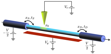
Figure 1: (Color online) Schematic setup of the 1D quantum dot, perturbed by the negatively charged AFM tip ($V_{t}<0$) at position $x_{0}$, capacitively coupled to the gate contact potential $V_{g}$ and connected, via tunnel barriers at positions $x_{S}=0$, $X_{D}=L$ with amplitudes $t_{S,D}$, to source $S$ and drain $D$ contacts, kept at a potential difference $V$.

The system is described by the Luttinger model with a free band linearized around the Fermi point $k_{F,s}=N_{s}^{(0)}\pi/L$, where $N_{s}^{(0)}$ is the reference number of electrons with spin $z$ component $s=\pm$ in the ground state. We consider here a reference state with an even total number $N_{+}^{(0)}=N_{-}^{(0)}$ and introduce $k_{F}\equiv k_{F,s}$. The odd case can be reproduced adding or subtracting one electron to the above case.

The dot Hamiltonian $H_{d}$ reads (from now on, $\hbar=1$)

$$H_{d}=H_{N}+H_{b},$$ (1)

with fabrizio

$$H_{N} = \frac{E_{\rho}}{2}(N_{\rho}-N_{g})^{2}+\frac{E_{\sigma}}{2}N_{\sigma}^{2},$$ (2)

$$H_{b} = \sum_{n_{q}>0}\left[\varepsilon_{\rho}n_{q}d^{\dagger}_{\rho,n_{q}}d_{\rho,n_{q}}+\varepsilon_{\sigma}n_{q}d^{\dagger}_{\sigma,n_{q}}d_{\sigma,n_{q}}\right]\,.$$ (3)

Here, $H_{N}$ represents the contribution of the zero modes

$$N_{\rho/\sigma}=N_{s=+}\pm N_{s=-}\,,$$ (4)

with $N_{s}$ the number of extra electrons with spin $s$, with respect to $N_{s}^{(0)}$. The energies $E_{\nu}=\pi v_{\nu}/2Lg_{\nu}$ have been introduced in terms of the velocity $v_{\nu}$ of the mode $\nu=\rho,\sigma$ and of the Luttinger parameters $g_{\nu}$. For repulsive interactions one has $g_{\rho}=g<1$, while $g=1$ corresponds to the noninteracting limit. On the other hand, $g_{\sigma}=1$ for an SU(2) invariant theory. voit The velocity of the charged mode is renormalized by the interactions and leads to $v_{\rho}=v_{F}/g$ where $v_{F}$ is the Fermi velocity. Within the standard Luttinger theory, the spin velocity is $v_{\sigma}=v_{F}$ even if, in more refined models, it may differ from this value. fiete1 ; fiete2 Furthermore, $N_{g}$ is the number of charges induced by a gate electrode capacitively coupled to the dot.
Note that the parameter $E_{\rho}$ might deviate from the simple expression quoted above due to e.g. screening induced by surrounding gates. Therefore, $E_{\rho}$ will be in the following treated as a free parameter with $E_{\rho}\gg E_{\sigma}$.
The term $H_{b}$ describes collective, quantized charge and spin density waves with boson operators $d_{\nu,n_{q}}$ and $\varepsilon_{\nu}=\pi v_{\nu}/L$, with $n_{q}\in\mathbb{N}$.
The electron field operator $\Psi_{s}(x)$ satisfying open boundary conditions $\Psi_{s}(0)=\Psi_{s}(L)=0$ is

$$\Psi_{s}(x)=e^{ik_{F}x}\psi_{s,+}(x)+e^{-ik_{F}x}\psi_{s,-}(x)\,,$$ (5)

where $\psi_{s,r}(x)$ are $2L$-periodic fermion fields representing right ($r=+$) and left ($r=-$) movers in the dot. Due to the open boundaries conditions one has $\psi_{s,r}(x)=-\psi_{s,-r}(-x)$. The right movers operator admits a bosonic representation fabrizio

$$\psi_{s,+}(x)=\frac{\eta_{s}}{\sqrt{2\pi\alpha}}e^{-i\theta_{s}}\,e^{i\frac{\pi N_{s}x}{L}}e^{i\frac{\Phi_{\rho}(x)+s\Phi_{\sigma}(x)}{\sqrt{2}}}\,.$$ (6)

Here, $\alpha$ is the cutoff length, of order $1/k_{F}$, $\theta_{s}$ satisfies $[\theta_{s},N_{s^{\prime}}]=i\delta_{s,s^{\prime}}$, and $\eta_{s}$ fulfill $\eta_{s}\eta_{s^{\prime}}+\eta_{s^{\prime}}\eta_{s}=2\delta_{s,s^{\prime}}$, allowing the right anticommutation relations for different spins. The boson fields $\Phi_{\rho}(x)$, $\Phi_{\sigma}(x)$ are given by

$$\Phi_{\nu}(x)=\sum_{n_{q}>0}\frac{e^{-\alpha q/2}}{\sqrt{g_{\nu}n_{q}}}\left[\left(\cos{(qx)}-ig_{\nu}\sin{(qx)}\right)d^{\dagger}_{\nu,n_{q}}+h.c.\right]$$

with $q=n_{q}\pi/L$.

The coupling with the AFM tip is modeled as a capacitive interaction

$$H_{tip}=-e\int_{0}^{L}dx\ V_{tip}(x)\rho(x)$$ (7)

between the electron density $-e\rho(x)$ and the tip potential $V_{tip}(x)$, peaked around $x_{0}$.

The particle density $\rho(x)=\sum_{s=\pm}\rho_{s}(x)$ with

$$\rho_{s}(x)=\Psi_{s}^{\dagger}(x)\Psi_{s}(x)$$ (8)

can be bosonized comm using Eqns. (5,6), one has ($\alpha=k_{F}^{-1}$)

$$\rho_{s}(x)=\frac{k_{F}}{\pi}+\frac{N_{s}}{L}-\frac{1}{\pi}\partial_{x}\varphi_{s}(x)+\rho_{s}^{F}(x)\,.$$ (9)

Here, the first three terms represent the long wave part expressed in terms of the antisymmetric field

$$\varphi_{s}(x) = \frac{\varphi_{\rho}(x)+s\varphi_{\sigma}(x)}{\sqrt{2}},$$ (10)

$$\varphi_{\rho/\sigma}(x) = \frac{1}{2}\left[\Phi_{\rho/\sigma}(-x)-\Phi_{\rho/\sigma}(x)\right]\,,$$ (11)

while the Friedel part $\rho_{s}^{F}(x)$ is given by shulz ; fabrizio

$$\rho_{s}^{F}(x) = -\frac{k_{F}}{\pi}\cos\left[\mathcal{L}(N_{s},x)-2\varphi_{s}(x)\right]\,,$$ (12)

$$\mathcal{L}(n,x) = 2k_{F}x+\frac{2\pi x}{L}n-2h(x)\,.$$ (13)

with

$$h(x)=\frac{1}{2}\tan^{-1}\left[\frac{\sin(2\pi x/L)}{e^{\pi\alpha/L}-\cos(2\pi x/L)}\right]\,.$$ (14)

In addition to the above terms, we will consider the so called Wigner contribution

$$\rho^{W}(x)\propto e^{-4ik_{F}x}\psi^{\dagger}_{+,+}(x)\psi_{+,-}(x)\psi^{\dagger}_{-,+}(x)\psi_{-,-}(x)+\mathrm{h.c.}$$

which arises from the presence of electron-electron interaction bortz beyond the Luttinger approximation, external perturbations, safi or by effects of ion-electron interactions. fiete1 Its bosonic form is shulz

$$\rho^{W}\!\!(x)\!=\!-\frac{Ak_{F}}{\pi}\!\!\cos\!\left[2\mathcal{L}(N_{\rho}/2,x)-2\sqrt{2}\varphi_{\rho}(x)\right]\,,$$ (15)

where $A$ is a model dependent constant. Note that, in contrast to the Friedel term, the Wigner one depends on the charge sector only. The coupling with the tip is then represented as $H_{tip}=H^{F}_{tip}+H^{W}_{tip}$, with

$$H^{F}_{tip} = V_{F}\sum_{s}\cos\!\left[\mathcal{L}(N_{s},x_{0})-2\varphi_{s}(x_{0})\right]$$ (16)

$$H^{W}_{tip} = V_{W}\cos\!\left[2\mathcal{L}(N_{\rho}/2,x_{0})-2\sqrt{2}\varphi_{\rho}(x_{0})\right]\,,$$ (17)

where $V_{F}$ and $V_{W}$ are free parameters that depend on the shape of the AFM tip and on the weight of the Friedel/Wigner oscillations. Note that we neglected the coupling with the long wavelength part of the density since it can be adsorbed in the Hamiltonian with a unitary transformation.

III Chemical potential

The presence of $H_{tip}$ shifts the energy levels of the quantum dot

$$E(N_{\rho},N_{\sigma},x_{0})=E^{0}(N_{\rho},N_{\sigma})+\langle H_{tip}(x_{0})\rangle$$ (18)

with respect to the bare case

$$E^{0}({N_{\rho},N_{\sigma}})=\frac{E_{\rho}}{2}(N_{\rho}-N_{g})^{2}+\frac{E_{\sigma}}{2}N_{\sigma}^{2}\,,$$ (19)

with $\langle\ldots\rangle$ the thermal average with respect to $H_{b}$ at fixed particle number. The average is decomposed in Friedel and Wigner terms, for $T\to 0$ one has

$$\langle H_{tip}(x_{0})\rangle=\sum_{\xi=F,W}E^{\xi}_{tip}(N_{\rho},N_{\sigma},x_{0})$$ (20)

with

$$\!\!\!\!\!\!E^{F}_{tip}(N_{\rho},N_{\sigma},x_{0})\!\! = \!\!V_{F}K^{F}(x_{0})\sum_{s=\pm}\cos\left[\mathcal{L}({N_{s}},x_{0})\right]\,,$$ (21)

$$\!\!\!\!\!\!E^{W}_{tip}(N_{\rho},N_{\sigma},x_{0})\!\! = \!\!V_{W}K^{W}(x_{0})\cos\left[2\mathcal{L}({N_{\rho}/2},x_{0})\right]\,,$$ (22)

where $K^{F}(x_{0})~{}=~{}\exp{[-2\langle\varphi_{s}^{2}(x_{0})\rangle]}$ and $K^{W}(x_{0})~{}=~{}\exp{[-4\langle\varphi_{\rho}^{2}(x_{0})\rangle]}$ with

$$K^{F}(x_{0}) = \left[\frac{\sinh\left({\frac{\pi\alpha}{2L}}\right)}{\sqrt{\sinh^{2}\left({\frac{\pi\alpha}{2L}}\right)+\sin^{2}\left(\frac{\pi x_{0}}{L}\right)}}\right]^{\frac{1+g}{2}}\,,$$ (23)

$$K^{W}(x_{0}) = \left[\frac{\sinh\left({\frac{\pi\alpha}{2L}}\right)}{\sqrt{\sinh^{2}\left({\frac{\pi\alpha}{2L}}\right)+\sin^{2}\left(\frac{\pi x_{0}}{L}\right)}}\right]^{2g}.$$ (24)

The chemical potential for a given configuration with $N_{\rho}$ charges and spin $N_{\sigma}$ is defined as

$$\mu_{d}(N_{\rho},N_{\sigma},x_{0})=E(N_{\rho}+1,N_{\sigma}\pm 1,x_{0})-E(N_{\rho},N_{\sigma},x_{0})$$ (25)

with $E(N)$ given in Eq. (18). The above expression holds either for ground states, where $N_{\rho}=0$ ($N_{\rho}=1$) for even (odd) $N$ ($N$ being the total number of particles) and

$$|N_{\sigma}|=\frac{1-(-1)^{N_{\rho}}}{2}\,,$$ (26)

and for excited states where $|N_{\sigma}|$ attains larger values with possibly $N_{\rho}>0$ ($N_{\rho}>1$) for an even (odd) $N$. The chemical potential can be decomposed as

$$\mu_{d}(N_{\rho},N_{\sigma},x_{0})=\mu_{0}(N_{\rho},N_{\sigma})+\delta\mu(N_{\rho},N_{\sigma},x_{0})\,,$$ (27)

where

$$\mu_{0}(N_{\rho},N_{\sigma})=E_{\rho}\left(\frac{1}{2}+N_{\rho}-N_{g}\right)+E_{\sigma}\frac{1\pm 2N_{\sigma}}{2}$$ (28)

is the bare dot chemical potential and

$$\delta\mu(N_{\rho},N_{\sigma},x_{0})=\sum_{\xi=F,W}\delta\mu^{\xi}(N_{\rho},N_{\sigma},x_{0})$$ (29)

are the corrections due to the tip. They have been the subject of numerical investigation sgm2 with exact diagonalization techniques in the regime of low $N_{\rho}$. As can be seen in Eq. (21) and Eq. (22), $\delta\mu^{\xi}(N_{\rho},N_{\sigma},x_{0})$ exhibits an oscillatory shape enveloped by $K^{\xi}(x_{0})$.
Let us now specify the above general expressions to the case involving ground states only, i.e. when Eq. (26) holds, relevant to study the linear transport regime. By exploiting the relation $2N_{s}=N_{\rho}+sN_{\sigma}$ it is easy to show that

$$\delta\mu^{F}(x_{0}) = V_{F}K^{F}(x_{0})\left\{\cos\left[\mathcal{L}(\mathcal{N}+1,x_{0})\right]-\cos\left[\mathcal{L}(\mathcal{N},x_{0})\right]\right\}\,,$$ (30)

$$\delta\mu^{W}(x_{0}) = V_{W}K^{W}(x_{0})\left\{\cos\left[2\mathcal{L}\left(\frac{N_{\rho}+1}{2},x_{0}\right)\right]-\cos\left[2\mathcal{L}\left(\frac{N_{\rho}}{2},x_{0}\right)\right]\right\}\,,$$ (31)

with

$$\mathcal{N}=\begin{cases}N_{\rho}/2&\mathrm{if}\ N_{\rho}\ \mathrm{is\ even}\\ (N_{\rho}-1)/2&\mathrm{if}\ N_{\rho}\ \mathrm{is\ odd}\\ \end{cases}$$ (32)

The corrections to the chemical potential present an oscillatory behavior given by the superposition of two cosine terms. For the Friedel case, if $N$ is even they oscillate with wavelength $2L/(N+2)$ and $2L/N$, while for odd $N$ their wavelength is $2L/(N+1)$ and $2L/(N-1)$. For the Wigner case, one always finds the spacial frequencies $L/(N+1)$ and $L/N$ .
These oscillating patterns are modulated by the functions $K^{F}(x_{0})$ and $K^{W}(x_{0})$. They depend both on the number of electrons through the cut-off $\alpha=k_{F}^{-1}$ and on the interaction parameter $g_{\rho}$, dictating their power-law scaling.
The interaction parameter $g$ dictates the relevance of the Wigner term in comparison to the Friedel one. By inspecting Eqns. (23,24) it is easy to show that Wigner correlations become relevant for $g<1/3$, see Ref. safi, .

In addition, as $N$ grows, $\alpha$ and thus $K^{\xi}(x_{0})$ are suppressed. In this limit quantum confinement effects become less relevant as the system crosses over towards the semi-classical regime. Furthermore, as the high-density limit is approached kinetic terms become more relevant than Coulomb repulsion, vignale leading to a further suppression of the signatures due to the Wigner molecule.

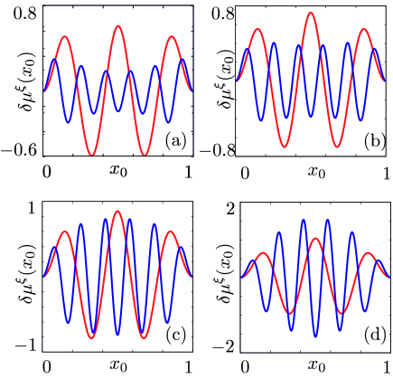
Figure 2: (Color online) Chemical potential corrections $\delta\mu^{\xi}(x_{0})$ (units $E_{\rho}$) as a function of $x_{0}$ (units $L$) for the transition $5\leftrightarrow 6$ and different values of the interaction parameter: (a) g=1; (b) g=0.7; (c) g=0.4; (d) g=0.1. Red (gray) curves represent the Friedel correction, blue (dark gray) curves the Wigner correction. In all panels, $V_{F}=V_{W}=\varepsilon_{\sigma}$ and $\alpha=k_{F}^{-1}=L/3\pi$.

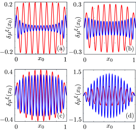
Figure 3: (Color online) Same as in Fig. 2 but for $16\leftrightarrow 17$ and $\alpha=k_{F}^{-1}=\pi/8L$.

The above analysis is confirmed by Figs. 2 and 3 which show the corrections to the chemical potential for $N=5$ and $N_{\rho}=16$ respectively, and different values of $g$. Indeed, for each of these cases it is clear that Wigner oscillations grow and eventually become relevant as $g\to 0$. Also, it is clear that for a given interaction strength both Friedel and Wigner oscillations get smaller as the number of partiles increases.

IV Transport

The coupling between the dot and the leads is produced by tunneling barriers at $x_{S}=0$ and $x_{D}=L$

$$H_{t}=\sum_{\lambda=S,D}\sum_{s=\pm}\left[t_{\lambda}\chi^{\dagger}_{s,\lambda}(x_{\lambda})\psi_{s,+}(x_{\lambda})+h.c.\right]=\sum_{\lambda}H_{t}^{\lambda}\,,$$

with $\chi_{s,\lambda}(x_{\lambda})$ ($\lambda=S,D$) the fermion operators at the end point of the lead $\lambda$ and $t_{\lambda}$ the transmission amplitudes of the tunnel barriers. The dot is subject to a symmetric voltage drop $V_{S}=-V/2$, $V_{D}=V/2$ between the two leads. The leads are modeled as non-interacting Fermi gases with $H_{leads}=H_{S}+H_{D}$ and we have set the bare leads chemical potential to zero.

The key quantities of transport in the sequential regime are the tunneling rates. They will be evaluated via the time evolution of the density operator.

At the initial time $t=0$ the dot is characterized by the state $|{\mathcal{S}}^{i}\rangle\equiv|N_{\rho}^{i},N_{\sigma}^{i}\rangle$. Here, we will consider the full dynamics of the zero modes while the bosonic excitations will be assumed in thermal equilibrium. The initial density operator then reads

$$\rho(0)=\frac{e^{-\beta\left(H_{S}+H_{D}\right)}}{Z_{S}Z_{D}}\frac{e^{-\beta H_{b}}}{Z_{b}}|\mathcal{S}^{i}\rangle\langle\mathcal{S}^{i}|\,,$$ (33)

with the partition functions $Z_{r}=Tr\left\{e^{-\beta H_{r}}\right\}$, $r\in\{b,S,D\}$ and $\beta=1/(k_{B}T)$. The probability ${\mathcal{P}}_{{{\mathcal{S}}^{i}}\rightarrow{{\mathcal{S}}^{f}}}(t)$ of finding the dot in the final state $|\mathcal{S}^{f}\rangle=|N^{f}_{\rho},N^{f}_{\sigma}\rangle$ at time $t$ is then obtained tracing out the leads and the bosonic degrees of freedom

$$\mathcal{P}_{{{\mathcal{S}}^{i}}\rightarrow{{\mathcal{S}}^{f}}}(t)=Tr\langle{\mathcal{S}}^{f}|\rho(t)|{\mathcal{S}}^{f}\rangle\,,$$ (34)

with $\rho(t)$ in the interaction picture blum with respect to $H^{(0)}=H_{d}+H_{leads}$

$$\rho(t)=\left[Te^{-i\int_{0}^{\tau}d\tau{\cal V}(\tau)}\right]\rho(0)\left[\widetilde{T}e^{i\int_{0}^{\tau}d\tau{\cal V}(\tau)}\right]\,.$$ (35)

Here, ${\mathcal{V}}(\tau)=e^{iH^{(0)}\tau}(H_{tip}+H_{t})e^{-iH^{(0)}\tau}$ and $T$ ($\widetilde{T}$) the time (anti-time) ordering operators. The probability in Eq. (34) is computed to the lowest order in the tunneling barriers and in the coupling to the AFM tip. The typical structure is

$$\mathcal{P}_{{{\mathcal{S}}^{i}}\rightarrow{{\mathcal{S}}^{f}}}(t)=\sum_{\lambda=S,D}\mathcal{P}_{{{\mathcal{S}}^{i}}\rightarrow{{\mathcal{S}}^{f}}}^{\lambda}(t)$$ (36)

with $\mathcal{P}_{{{\mathcal{S}}^{i}}\rightarrow{{\mathcal{S}}^{f}}}^{\lambda}(t)=\mathcal{P}_{{{\mathcal{S}}^{i}}\rightarrow{{\mathcal{S}}^{f}}}^{0,\lambda}(t)+\delta\mathcal{P}_{{{\mathcal{S}}^{i}}\rightarrow{{\mathcal{S}}^{f}}}^{\lambda}(t)$ and

$$\mathcal{P}_{{{\mathcal{S}}^{i}}\rightarrow{{\mathcal{S}}^{f}}}^{0,\lambda}(t) \!=\! \int_{0}^{t}dt_{1}\int_{0}^{t}dt_{2}F_{0}^{\lambda}(t_{1},t_{2}),$$ (37)

$$\delta\mathcal{P}_{{{\mathcal{S}}^{i}}\rightarrow{{\mathcal{S}}^{f}}}^{\lambda}(t) \!=\! \int_{0}^{t}\!dt_{1}\!\int_{0}^{t}\!dt_{2}\!\int_{0}^{t_{2}}\!\!\!dt_{3}\!\!\!\sum_{i=1,2}\!F_{i}^{\lambda}(t_{1},t_{2},t_{3})+c.c.\ ,$$ (38)

where

$$F_{0}^{\lambda}(t_{1},t_{2}) \!\!\!=\! Tr\langle\mathcal{S}^{f}|H_{t}^{\lambda}(t_{1})\rho(0)H_{t}^{\lambda}(t_{2})|\mathcal{S}^{f}\rangle,$$ (39)

$$F_{1}^{\lambda}(t_{1},\!t_{2},\!t_{3}) \!\!\!=\!\! iTr\langle\mathcal{S}^{f}|H_{t}^{\lambda}(t_{1})\rho(0)H_{t}^{\lambda}(t_{3})H_{tip}(t_{2})|\mathcal{S}^{f}\rangle,$$ (40)

$$F_{2}^{\lambda}(t_{1},\!t_{2},\!t_{3}) \!\!\!=\!\! iTr\langle\mathcal{S}^{f}|H_{t}^{\lambda}(t_{1})\rho(0)H_{tip}(t_{3})H_{t}^{\lambda}(t_{2})|\mathcal{S}^{f}\rangle\,.$$ (41)

Note that in the sequential tunneling limit considered in this paper the selection rules $|N_{\rho}^{f}-N_{\rho}^{i}|=|N_{\sigma}^{f}-N_{\sigma}^{i}|=1$ apply. In the following, we will focus on the case where only two charge states are involved in the transport.
The rates are given by the long time limit of the time derivate of $\mathcal{P}^{\lambda}(t)$

$$\Gamma_{\mathcal{S}^{i}\to\mathcal{S}^{f}}^{\lambda}=\lim_{t\rightarrow\infty}\dot{\mathcal{P}}_{\mathcal{S}^{i}\to\mathcal{S}^{f}}^{\lambda}(t)\,.$$ (42)

Their explicit evaluation, within the bosonization formalism, is presented in detail in Appendix A. Here we quote the main results. The rates have the general expression

$$\Gamma_{\mathcal{S}^{i}\to\mathcal{S}^{f}}^{\lambda}=\Gamma_{\mathcal{S}^{i}\to\mathcal{S}^{f}}^{0,\lambda}+\delta\Gamma_{\mathcal{S}^{i}\to\mathcal{S}^{f}}^{F,\lambda}(x_{0})+\delta\Gamma_{\mathcal{S}^{i}\to\mathcal{S}^{f}}^{W,\lambda}(x_{0})\,,$$ (43)

with

$$\Gamma_{\mathcal{S}^{i}\to\mathcal{S}^{f}}^{0,\lambda}=\Gamma_{0}^{\lambda}\sum_{q_{\rho},q_{\sigma}}A_{q_{\rho},q_{\sigma}}f\left[\Delta E_{\lambda}+q_{\rho}\varepsilon_{\rho}+q_{\sigma}\varepsilon_{\sigma}\right]$$ (44)

representing the tunneling rate in the absence of the tip apart from the full chemical potential including tip corrections and

$$\delta\Gamma_{\mathcal{S}^{i}\to\mathcal{S}^{f}}^{\xi,\lambda}(x_{0})=2V_{\xi}\Gamma_{0}^{\lambda}K^{\xi}(x_{0})\sum_{q_{\rho},q_{\sigma}}A_{q_{\rho},q_{\sigma}}R_{q_{\rho},q_{\sigma}}^{\xi,\lambda}(x_{0})$$ (45)

being the explicit corrections induced by the tip. Here, $\Gamma_{0}^{\lambda}=\nu_{0}\left|t_{\lambda}\right|^{2}/\pi\alpha$ with $\nu_{0}$ the leads density of states and $\Delta E_{\lambda}=\Delta neV_{\lambda}+\mu_{d}(N_{\rho}^{i},N_{\sigma}^{i},x_{0})$ with $\Delta n=(N_{\rho}^{f}-N_{\rho}^{i})$ and $\mu_{d}(N_{\rho}^{i},N_{\sigma}^{i},x_{0})$ defined in Eq. (25). The coefficients $A_{q_{\rho},q_{\sigma}}$ and $R_{q_{\rho},q_{\sigma}}^{\xi,\lambda}(x_{0})$ are respectively defined in Eq. (79) and Eq. (81).
The above rates fulfill the detailed balance relation

$$\Gamma_{\mathcal{S}^{i}\to\mathcal{S}^{f}}^{\lambda}=e^{-\beta\Delta E_{\lambda}}\Gamma_{\mathcal{S}^{f}\to\mathcal{S}^{i}}^{\lambda}\,.$$ (46)

The framework developed here is very general and allows to address both linear and nonlinear transport. haupt ; piovano In the rest of the paper, however, we will focus on the linear transport regime which already shows a rich and interesting physics. The nonlinear regime will be the subject of forthcoming investigations.

In the linear regime only two charge values $N$ and $N+1$ will be considered, with the correponding ground state spins. Namely,

$$|N_{\rho}=0,N_{\sigma}=0\rangle\quad \quad|N_{\rho}=1,N_{\sigma}=\pm 1\rangle\ (N\ \textrm{even})\,,$$ ;

$$|N_{\rho}=0,N_{\sigma}=\pm 1\rangle\quad \quad|N_{\rho}=1,N_{\sigma}=0\rangle\ (N\ \textrm{odd})\,.$$ ;

Note that in the absence of magnetic field, states with $N_{\sigma}=\pm 1$ are degenerate.
The standard expression for the linear conductance, expressed in terms of the rates involving the above states, is braggioepl

$$G=\left.\frac{\beta e^{2}D_{N}D_{N+1}\Gamma_{N\to N+1}^{S}\Gamma_{N+1\to N}^{D}}{D_{N}\Gamma_{N+1\to N_{\rho}}+D_{N+1}\Gamma_{N\to N+1}}\right|_{V=0}\,,$$ (48)

where $\Gamma_{N_{\rho}\to N_{\rho}^{\prime}}^{\lambda}$ is a shorthand notation for $\Gamma_{\mathcal{S}^{i}\to\mathcal{S}^{f}}^{\lambda}$, $D_{N}=\left[3+(-1)^{N+1}\right]/2$ is the degeneracy of the dot ground state with $N$ electrons and

$$\Gamma_{N_{\rho}\to N_{\rho}^{\prime}}=\Gamma_{N_{\rho}\to N_{\rho}^{\prime}}^{S}+\Gamma_{N_{\rho}\to N_{\rho}^{\prime}}^{D}\,.$$

The behavior of the conductance as a function of the external parameters will be numerically investigated in detail in the next section. Here we discuss a useful analytical approximation valid at low temperatures around the maximum of the conductance peak which is centered beenakker at $\mu_{d}(N_{\rho},N_{\sigma},x_{0})=0$ for $T=0$. As shown in Appendix A, in this regime the tunneling rates can be approximated as

$$\Gamma_{N_{\rho}\to N_{\rho}+1}^{\lambda}=\gamma^{\lambda}(x_{0})f(\mu)\ ;\ \Gamma_{N_{\rho}+1\to N_{\rho}}^{\lambda}=\gamma^{\lambda}(x_{0})f(-\mu)\\$$

where $f(E)$ is the Fermi function, $\mu\equiv\mu_{d}(N_{\rho},N_{\sigma},x_{0})$ is the dot chemical potential and $\gamma^{\lambda}(x_{0})$ is defined in Eq. (89). Employing the above expressions and the detailed balance in Eq. (46), one can rewrite the conductance as

$$G\approx\beta e^{2}D_{N}\Delta(x_{0})\frac{f(-\mu)}{1+(D_{N}/D_{N+1})e^{\beta\mu}}\,,$$ (49)

with

$$\Delta(x_{0})=\frac{\gamma^{S}(x_{0})\gamma^{D}(x_{0})}{\gamma^{S}(x_{0})+\gamma^{D}(x_{0})}\,.$$ (50)

Equation (49) describes a resonance peak located at

$$\mu=\frac{k_{B}T}{2}\log\left(\frac{D_{N+1}}{D_{N}}\right)\,.$$ (51)

When expressed in terms of $N_{g}$, the resonance is at

$$N_{g}=N_{g}^{*}+\frac{\delta\mu(x_{0})}{E}$$ (52)

with

$$N_{g}^{*}=N+\frac{1}{2}+\frac{E_{\sigma}}{2E_{\rho}}(-1)^{N_{\rho}}-\frac{k_{B}T}{2}\log{\left(\frac{D_{N_{\rho}+1}}{D_{N_{\rho}}}\right)}$$ (53)

and $\delta\mu(x_{0})$ given in Eq. (29). Therefore, the position of the conductance oscillates due to the tip-induced spatial fluctuations of the chemical potential.
Besides the oscillations of the peak position, also the amplitude of the conductance peak exhibits a modulation depending on the location of the tip: on resonance, the conductance evaluates to

$$G_{\mathrm{res}}=\beta e^{2}\frac{D_{N}D_{N+1}}{\left(\sqrt{D_{N}}+\sqrt{D_{N+1}}\right)^{2}}\Delta(x_{0})\,,$$ (54)

and thus explicitly depends on $x_{0}$ via the term $\Delta(x_{0})$. Such modulation has not been reported so far. sgm2 ; linear The term $\Delta(x_{0})$ can be expanded to within linear terms in $\delta\Gamma^{\xi,\lambda}$. Assuming symmetric tunnel barriers with $\Gamma_{0}^{\lambda}=\Gamma_{0}$, one has $\Delta(x_{0})\approx\Delta_{0}+\Delta_{1}^{F}(x_{0})+\Delta_{1}^{W}(x_{0})$ with

$$\Delta_{0}=\frac{\Gamma_{0}}{2}\left(1-e^{\frac{-\pi\alpha}{L}}\right)^{-\frac{1+g}{2}}\,,$$ (55)

and

$$\Delta_{1}^{\xi}(x_{0})=2\Delta_{0}V_{\xi}K^{\xi}(x_{0})\sum_{\nu=c,s}F_{\nu}^{\xi}(x_{0})g_{\nu}^{\xi}(x_{0})\,.$$ (56)

Here,

$$\!\!\!\!\!\!g_{c}^{F}(x_{0}) = \cos{\left[\frac{2\pi(\mathcal{N}+1)}{L}x-2h(x)+2k_{F}x\right]}+\cos{\left[\frac{2\pi\mathcal{N}}{L}x-2h(x)\right]}\,,$$ (57)

$$\!\!\!\!\!\!g_{s}^{F}(x_{0}) = \sin{\left[\frac{2\pi(\mathcal{N}+1)}{L}x-2h(x)+2k_{F}x\right]}-\sin{\left[\frac{2\pi\mathcal{N}}{L}x-2h(x)\right]}\,,$$ (58)

with $\mathcal{N}$ defined in Eq. (32). The functions $g_{c,s}^{W}$ have the same functional form after the replacements $\mathcal{N}\to N$ and $h(x)\to 2h(x)$. The weighting functions $F_{c,s}(x_{0})$ are given by

$$F_{c}^{\xi}(x_{0}) = \sum_{\mathbf{m}}\frac{B_{\mathbf{0},\mathbf{m}}^{\xi}}{\Lambda}\left\{\cos(kx_{0})+\cos\left[k(1-x_{0})\right]\right\}\,,$$ (59)

$$F_{s}^{\xi}(x_{0}) = \sum_{\mathbf{m}}\frac{B_{\mathbf{0},\mathbf{m}}^{\xi}}{\Lambda}\left\{\sin(kx_{0})-\sin\left[k(1-x_{0})\right]\right\}\,,$$ (60)

with $\mathbf{m}=\{m_{1},m_{2},m_{3},m_{4}\}$, $m_{i}\in\mathbb{N}$ and $m_{i}\geq 0$, $B_{\mathbf{n},\mathbf{m}}^{\xi}$ defined in Eqns. (84,85), $\Lambda=\varepsilon_{\rho}(m_{1}+m_{2})+\varepsilon_{\sigma}(m_{3}+m_{4})$, $k=\pi(m_{1}-m_{2}+m_{3}-m_{4})/L$ and the summations are extended over the set of $\mathbf{m}\neq\{0,0,0,0\}$.
It can be shown that $\Delta_{1}^{\xi}(x_{0})=\Delta_{1}^{\xi}(L-x_{0})$ and that $\Delta_{1}^{\xi}(L/2)=0$, therefore the amplitude modulations are symmetric around the center of the dot and vanish there.

V Results

In this section we discuss the behavior of the linear conductance in Eq. (48). The full numerical results will be interpreted with the aid of the analyltical expressions developed in Sec. IV.
We start considering a weakly interacting dot.

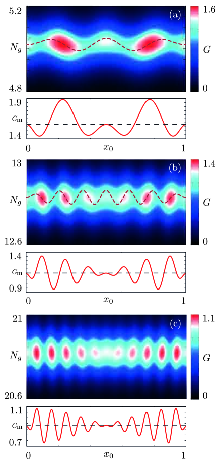
Figure 4: (Color online) Color-map plot of the linear conductance $G$ (units $e^{2}\Gamma_{0}/\varepsilon_{\sigma}$) as a function of $N_{g}$ and $x_{0}$ (units $L$) and plot of the conductance peak maximum $G_{\mathrm{m}}$ as a function of $x_{0}$ (units $L$) for a transition $N\leftrightarrow N+1$ with (a) $N=5$; (b) $N=12$; (c) $N=20$. The dashed lines superimposed to the color-maps represent the calculated chemical potential traces - see Eqns. (29,30,31) - the ones in the amplitude plots signal the value of the bare conductance peak obtained in the absence of the tip. Here, only the Friedel corrections have been included, with $V_{F}=0.07\varepsilon_{\sigma}$ and $V_{W}=0$. Other parameters are $k_{B}T=0.05\varepsilon_{\sigma}$, $E_{\rho}=5E_{\sigma}$ and $g=0.9$.

Figure 4 shows the conductance for $g=0.9$ and three transitions $5\leftrightarrow 6$, $12\leftrightarrow 13$ and $20\leftrightarrow 21$. For this calculation we have included only the corrections due to Friedel oscillations as one can expect that the Wigner term represents a vanishing perturbation due to $V_{W}\to 0$ in this limit. bortz The main panels show the conductance with a colorscale plot, as a function of the tip position $x_{0}$ and $N_{g}$. Below the density plot the maximum of the linear conductance, $G_{\mathrm{m}}$, is shown as a function of $x_{0}$. Two main features are observed, namely

($i$) oscillations of its position,
($ii$) oscillations of its height.

The fact ($i$) is in agreement with previous findings. sgm2 ; linear The fluctuations of the conductance peak position turn out to be proportional to the tip-induced correction to the chemical potential $\delta\mu(x_{0})\equiv\delta\mu^{F}(x_{0})$ in this case - see Eqns. (29,30). Indeed, the oscillations of the resonance position exhibit a number of maxima and minima in accordance with the discussion in Sec. III. This confirms the analytical prediction shown in Sec. IV, see Eq. (52). As a specific example, for the case of the transition $5\leftrightarrow 6$ the plot in panel (a) exhibits three maxima and two minima.

More interesting is the modulation of the height of the linear conductance which has never been reported so far. This modulation is sizeable and could be detected in a transport experiment. It exhibits a symmetric, beating-like pattern. The beating phenomenon is particularly evident as $N$ increases. This fact will be analyzed in more detail later in this section.

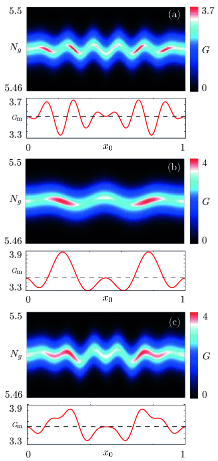
Figure 5: (Color online) Color-map plot of the linear conductance (units $e^{2}\Gamma_{0}/\varepsilon_{\sigma}$) for the transition $N=5\leftrightarrow 6$ as a function of $N_{g}$ and $x_{0}$ (units $L$) and plot of the conductance peak maximum $G_{\mathrm{m}}$ as a function of $x_{0}$ (units $L$) calculated with (a) $V_{F}=0$, $V_{W}=0.07\varepsilon_{\sigma}$; (b) $V_{F}=0.07\varepsilon_{\sigma}$, $V_{W}=0$; (c) $V_{F}=V_{W}=0.07\varepsilon_{\sigma}$. Other parameters are $k_{B}T=0.05\varepsilon_{\sigma}$, $E_{\rho}=5E_{\sigma}$ and $g=0.2$.

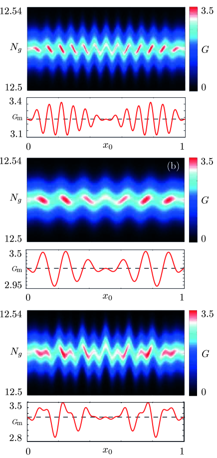
Figure 6: (Color online) Same plot as in Fig. 5 but for the transition $N=12\leftrightarrow 13$ for (a) $V_{F}=0$, $V_{W}=0.07$; (b) $V_{F}=0.07$, $V_{W}=0$; (c) $V_{F}=V_{W}=0.07\varepsilon_{\sigma}$. Other parameters are $k_{B}T=0.05\varepsilon_{\sigma}$, $E_{\rho}=5E_{\sigma}$ and $g=0.2$.

Let us now turn to the case of stronger interactions and study the effects due to the Wigner corrections. Figures 5 and 6 show the linear conductance for $g=0.3$ and the transitions $5\leftrightarrow 6$ and $12\leftrightarrow 13$ respectively. Panels (a) and (b) show the Wigner and the Friedel contributions to the conductance. While the Friedel corrections follow the pattern discussed above, Wigner corrections exhibit a shorter wavelength with precisely $N+1$ maxima and $N$ minima, double the number of those observed in the Friedel case. The position of the conductance peak in the Wigner case follows the position-dependent correction to the chemical potential $\delta\mu^{W}(x_{0})$ defined in Eq. (31). Friedel and Wigner corrections induce therefore oscillatory patterns with very different wavelengths, allowing to distinguish the two mechanisms in a non-ambiguous way. Although we have shown the two contributions separately, it can be in general expected that the Wigner and the Friedel mechanisms co-exist. Therefore, in panels (c) we show the conductance in the presence of both perturbations, considering the case of equal amplitudes. Even if here we have chosen the same weights for the Friedel and the Wigner terms ($V_{F}=V_{W}$), the latter impresses its peculiar oscillatory pattern with wavelength $\approx L/N$ on the conductance peak position. Indeed, as we have already observed in Sec. III, when interactions increase the Wigner contribution to the chemical potential becomes even more relevant than the Friedel one. This explains the persistence of $N+1$ maxima and $N$ minima in the oscillations of the chemical potential. Also conductance amplitudes exhibit a pattern reminiscent of the $N+1$ and $N$ maxima and minima but less pronounced with respect to the one shown in the position of the conductance peak.

Let us now investigate the stability of these findings as a function of the strength of interactions.

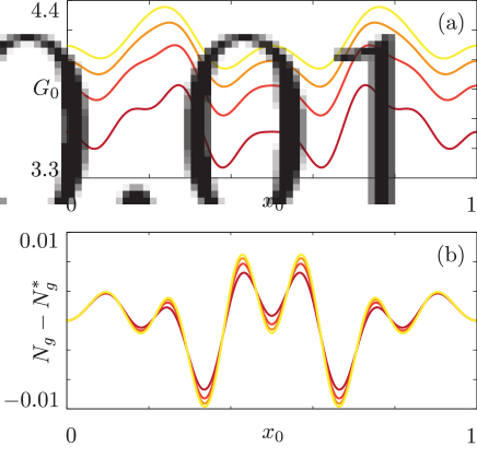
Figure 7: (Color online) For the transition $5\leftrightarrow 6$ (a) Conductance maximum $G_{\mathrm{m}}$ (units $e^{2}\Gamma_{0}/\varepsilon_{\sigma}$) and (b) position offset $N_{g}-N_{g}^{*}$ - see Eq. (52) - of the conductance peak as a function of $x_{0}$ (units $L$) and several values of the interaction parameter $g=0.2,\ 0.1,\ 0.05,\ 0.02$ (from darker to lighter color). Here we have chosen $V_{F}=V_{W}=0.07\varepsilon_{\sigma}$. Other parameters as in Fig. 5.

Figure 7 shows the linear conductance maximum and position for the transition $5\leftrightarrow 6$ as a funciton of $x_{0}$ for several values of the Luttinger parameter $g$. As interactions grow, and $g\to 0$, two striking features are observed. While the oscillations of the chemical potential always exhibit six maxima and five minima, with an increase in the peak-to-valley ratio, the oscillations due to the Wigner contribution in the peak amplitude tend to vanish.
Therefore, the effect of the Wigner corrections to the chemical potential and to the peak amplitude are very different: in the former case Wigner contributions are stable against Coulomb interactions, while Wigner corrections to the conductance maximum become vanishing for $g\to 0$.

In order to interpret the oscillations of $G_{\mathrm{m}}$, let us turn to the analytic model developed in Sec. IV. The height of the conductance peak follows $\Delta_{1}^{\xi}(x_{0})$, given in Eq. (56). It is composed by the sum of two beating patterns, the terms $g_{c,s}^{\xi}(x_{0})$, enveloped by the slow functions $F_{c,s}^{\xi}(x_{0})$.

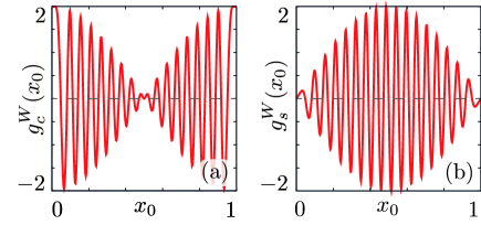
Figure 8: (Color online) (a) Plot of $g_{c}^{W}(x_{0})$ as a function of $x_{0}$ (units $L$) for $N=16$ and $\alpha=k_{F}^{-1}=\pi/8L$; (b) Same as in (a) but for $g_{s}^{W}(x_{0})$.

The beatings arise from the superposition of the two cosine or sine terms occurring in $g_{c,s}^{\xi}(x_{0})$ with a wavelength difference of $2\pi/L$ and is therefore especially clear when $N\gg 1$. Figure 8 shows a typical example for the case of the Wigner correction. The Friedel case is perfectly analogous, only with half the wavelength.

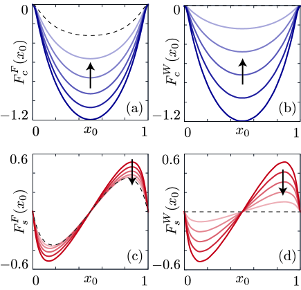
Figure 9: (Color online) (a) Plot of $F_{c}^{F}(x_{0})$ (units $\varepsilon_{\sigma}^{-1}$) as a function of $x_{0}$ (units $L$) for different values of $g=1,\ 0.8,\ 0.6,\ 0.4,\ 0.2$ (from darker to lighter color). The arrow denotes the evolution of the family of curves as $g$ decreases (interaction strength increases); (b) Same as in (a) but for $F_{c}^{W}(x_{0})$; (c) Same as in (a) but for $F_{s}^{F}(x_{0})$; (c) Same as in (a) but for $F_{s}^{W}(x_{0})$. The dashed curve represents the asymptotic case $g\to 0$. All panels have been plotted for $N=16$.

The envelope functions $F_{c,s}^{\xi}(x_{0})$ parametrically depend on $g$ and only very weakly on $N$ through the cutoff $\alpha$. They are plotted in Fig. 9. The overall shape of the Friedel and Wigner cases is analogous. Important differences however arise when the interaction strength increases ($g\to 0$). While $F_{c,s}^{F}(x_{0})$ tend asymptotically to a limit function, the terms $F_{c,s}^{W}(x_{0})\to 0$. The mathematical origin of this fact lies in the factor $\Lambda^{-1}$ into the summations defining Eqns. (59,60). Indeed, see Appendix A, for the Wigner case $\Lambda\propto\varepsilon_{\rho}\propto g^{-1}$ and thus $F_{c,s}^{W}(x_{0})\to 0$ as $g\to 0$. On the other hand, for the Friedel case $\Lambda$ depends both on $\varepsilon_{\rho}$ and $\varepsilon_{\sigma}$ and thus non-vanishing contributions are still present even in the regime of very strong interactions.
This confirms that the effects of the Friedel oscillations on the conductance peak amplitude seem more robust again the ones induced by Wigner oscillations. The rather counter-intuitive conclusion that the corrections to the maximum value of the linear conductance due to the Wigner term vanish in the $g\to 0$ limit is very interesting. We want to remind however that our discussion here concerns the intrinsic dependence on the interaction parameter, regardless the weighting factors of $\rho^{F,W}(x)$.

VI Conclusions

In this paper we have calculated the transport properties of an interacting one-dimensional quantum dot, described by means of the Luttinger liquid theory, in the presence of an AFM tip capacitively coupled to it. We have considered both Friedel and Wigner corrections to the electron density and evaluated their contributions both to the chemical potential and to the tunneling rates to the lowest order in the AFM-dot coupling.
To discuss the transport properties we have focused on the linear regime, where we have shown that the AFM tip induces a shift of the conductance peak and a renormalization of the conductance strength, which has never been discussed in previous works on this subject. Scanning the tip along the dot allows to observe oscillatory patterns related to both the Friedel and the Wigner oscillations of the electron density. A beating pattern emerges in the linear conductance height oscillations. The Friedel and the Wigner contributions show markedly distinct wavelengths allowing in principle to distinguish the two effects. Surprisingly, we have found that as the interaction strength grows, the effects of the Wigner oscillations on the conductance height vanish, while those on the oscillations of the peak position are reinforced.
Interesting effects are expected to show up even in the nonlinear transport regime, also in connection to the possibility to trigger and probe dot excited states. This will be the subject of forthcoming investigations.

Acknowledgments. Financial support by the EU- FP7 via ITN-2008-234970 NANOCTM is gratefully acknowledged.

Appendix A Tunneling rate

In this Appendix we outline the calculation of the tunneling rates $\Gamma_{\mathcal{S}^{i}\to\mathcal{S}^{f}}^{\lambda}$ introduced in Sec. IV, where $|\mathcal{S}_{i,f}\rangle=|N_{\rho}^{i,f},N_{\sigma}^{i,f}\rangle$.
Let us start with the term $F_{0}^{\lambda}(t_{1},t_{2})$ in Eq. (39). Following standard procedures already outlined in literature ioale1 ; ioale2 one obtains the standard result

$$F_{0}^{\lambda}(t_{1},t_{2})=\frac{\left|t_{\lambda}\right|^{2}}{2\pi\alpha}e^{-i\Delta E_{\lambda}(t_{2}-t_{1})}e^{-W_{\lambda}(t_{2}-t_{1})}e^{-W_{d}(t_{2}-t_{1})}$$

where

$$\Delta E_{\lambda}^{0}=\Delta neV_{\lambda}+\mu_{0}(N_{\rho}^{i},N_{\sigma}^{i})$$ (61)

with $\Delta n=(N_{\rho}^{f}-N_{\rho}^{i})$ and $\mu_{0}(N_{\rho}^{i},N_{\sigma}^{i})$ is the bare chemical potential of the dot, see Eq. (28).
Note that we have introduced the full chemical potential, including tip-induced corrections. The kernel

$$e^{-W_{\lambda}(\tau)}=\langle\chi_{s,\lambda}^{\dagger}(x_{\lambda},\tau)\chi_{s,\lambda}(x_{\lambda},0)\rangle_{leads}$$ (62)

is the correlation function for lead $\lambda$, which can be written as

$$e^{-W_{\lambda}(\tau)}=\nu_{\lambda}\int_{-\infty}^{\infty}\ dE\ e^{iE\tau}f(E)\,,$$ (63)

with $\nu_{\lambda}$ the density of states in lead $\lambda$ and

$$f(E)=\frac{1}{1+e^{\beta E}}$$ (64)

is the Fermi function. In the following we will assume $\nu_{\lambda}\equiv\nu_{0}$. Concerning the dot, $e^{-W_{d}(\tau)}$ stems from the thermal average over the collective excitations of the initial states and sum over the final ones with ioale1 ; ioale2 ; iotobias

$$W_{d}(\tau)=\frac{1}{2}\left[\frac{1}{g}W\left(\varepsilon_{\rho},\tau\right)+W\left(\varepsilon_{\sigma},\tau\right)\right]\,,$$ (65)

where

$$W(\varepsilon,\tau) = \sum_{n>0}\frac{e^{-\pi\alpha n/L}}{n}\left[\coth{\left(\frac{\beta n\varepsilon}{2}\right)}\left(1-\cos(n\varepsilon\tau)\right)\right.$$ (66)

$$+ \left.i\sin(n\varepsilon\tau)\right]\,.$$

The perturbation terms $F_{1,2}^{(\lambda)}(t_{1},t_{2},t_{3})$ in Eqns. (40,41) can be decomposed into Friedel ($\xi=F$) and Wigner ($\xi=W$) parts

$$F_{j}^{\lambda}(t_{1},t_{2},t_{3})=\sum_{\xi=F,W}F_{j}^{\xi,\lambda}(t_{1},t_{2},t_{3})\,,$$ (67)

with

$$F_{1}^{\xi,\lambda}(t_{1},t_{2},t_{3}) = -i\frac{V_{\xi}}{\pi\alpha}K^{\xi}(x_{0})F_{0}^{\lambda}(t_{1},t_{3})\cos{\left[\mathcal{L}_{\xi}^{f}(X_{\lambda})+\Delta\mathcal{G}_{1}^{\xi,\lambda}(t_{1},t_{2},t_{3})\right]}$$ (68)

$$F_{2}^{\xi,\lambda}(t_{1},t_{2},t_{3}) = -i\frac{V_{\xi}}{\pi\alpha}K^{\xi}(x_{0})F_{0}^{\lambda}(t_{1},t_{3})\cos{\left[\mathcal{L}_{\xi}^{i}(X_{\lambda})+\Delta\mathcal{G}_{2}^{\xi,\lambda}(t_{1},t_{2},t_{3})\right]}$$ (69)

where $X_{S}=x_{0}$, $X_{D}=L-x_{0}$, $K^{\xi}(x_{0})$ are defined in Eqns. (23,24) and

$$\mathcal{L}_{F}^{i/f}(x) = \Delta n\mathcal{L}(N_{s}^{i/f},x)\,;$$ (70)

$$\mathcal{L}_{W}^{i/f}(x) = 2\Delta n\mathcal{L}(N_{\rho}^{i/f}/2,x)\,.$$ (71)

The functions

$$-i\Delta\mathcal{G}_{j}^{\xi,\lambda}(t_{1},t_{2},t_{3})=(-1)^{j}\mathcal{G}_{\xi}^{\lambda}(t_{3}-t_{2})-\mathcal{G}_{\xi}^{\lambda}(t_{1+j}-t_{1})\,,$$

with $j\in\{1,2\}$, are expressed in terms of

$$\mathcal{G}_{F}^{\lambda}(\tau) = -\frac{1}{2}\sum_{\nu=\rho,\sigma}\sum_{p=\pm 1}pW\left(\varepsilon_{\nu},\tau+\frac{X_{\lambda}}{v_{\nu}}\right)\,,$$ (72)

$$\mathcal{G}_{W}^{\lambda}(\tau) = -\sum_{p=\pm 1}pW\left(\varepsilon_{\rho},\tau+\frac{X_{\lambda}}{v_{\rho}}\right)\,.$$ (73)

Since $W(u)$ is periodic, it is convenient to exploit the Fourier series

$$e^{\pm\kappa W(u)}=\sum_{l=-\infty}^{\infty}b_{l}^{\pm,\kappa}e^{-ilu}\,.$$ (74)

For $k_{B}T\ll\varepsilon_{\sigma}$ one can approximate $W_{l}$ with their expression ioale1 ; ioale2 calculated for $T=0$,

$$b_{l}^{+,\kappa} = \left(-e^{-\frac{l\pi\alpha}{L}}\right)^{l}\left(1-e^{-\frac{\alpha\pi}{L}}\right)^{\kappa}\frac{\Gamma(1+\kappa)\theta(l)}{l!\Gamma(1+\kappa-l)}$$ (75)

$$b_{l}^{-,\kappa} = \left(e^{-\frac{l\pi\alpha}{L}}\right)^{l}\left(1-e^{-\frac{\alpha\pi}{L}}\right)^{-\kappa}\frac{\Gamma(l+\kappa)}{l!\Gamma(\kappa)}\theta(l),$$ (76)

where $\Gamma(x)$ is the Euler gamma function. Inserting Eq. (68) and Eq. (69) into Eq. (37) and Eq. (38) it is possible to perform the time integration exploiting the above Fourier expansions.
The tunneling rate in Eq. (42) can be written as

$$\Gamma_{\mathcal{S}^{i}\to\mathcal{S}^{f}}^{\lambda}=\Gamma_{\mathcal{S}^{i}\to\mathcal{S}^{f}}^{0,\lambda}+\delta\Gamma_{\mathcal{S}^{i}\to\mathcal{S}^{f}}^{F,\lambda}(x_{0})+\delta\Gamma_{\mathcal{S}^{i}\to\mathcal{S}^{f}}^{W,\lambda}(x_{0})\,,$$ (77)

with

$$\Gamma_{\mathcal{S}^{i}\to\mathcal{S}^{f}}^{0,\lambda}=\Gamma_{0}^{\lambda}\sum_{q_{\rho},q_{\sigma}}A_{q_{\rho},q_{\sigma}}f\left[\Delta E_{\lambda}^{0}+q_{\rho}\varepsilon_{\rho}+q_{\sigma}\varepsilon_{\sigma}\right]$$ (78)

where $\Gamma_{0}^{\lambda}=\nu_{\lambda}\left|t_{\lambda}\right|^{2}/\pi\alpha$ and

$$A_{q_{\rho},q_{\sigma}}=b^{-,g/2}_{q_{\rho}}b^{-,1/2}_{q_{\sigma}}\,;$$ (79)

the corrections induced by the tip read

$$\delta\Gamma_{\mathcal{S}^{i}\to\mathcal{S}^{f}}^{\xi,\lambda}(x_{0}) = 2V_{\xi}\Gamma_{0}^{\lambda}K^{\xi}(x_{0})\sum_{q_{\rho},q_{\sigma}}A_{q_{\rho},q_{\sigma}}R_{q_{\rho},q_{\sigma}}^{\xi,\lambda}(x_{0})$$ (80)

$$+ \left[\sum_{q_{\rho},q_{\sigma}}A_{q_{\rho},q_{\sigma}}\partial_{eV_{\lambda}}f(\Delta E_{\lambda}^{0}+q_{\rho}\varepsilon_{\rho}+q_{\sigma}\varepsilon_{\sigma})\right]V_{\xi}K^{\xi}(x_{0})\left\{\cos\left[\mathcal{L}_{\xi}^{f}(x_{0})\right]-\cos\left[\mathcal{L}_{\xi}^{i}(x_{0})\right]\right\}$$

where

$$\!\!\!\!\!\!\!\!\!\!R_{q_{\rho},q_{\sigma}}^{\xi,\lambda}(x_{0}) = \left\{\sum_{\mathbf{n},\mathbf{m}|\Lambda\neq 0}\frac{B^{\xi}_{\mathbf{n},\mathbf{m}}}{\Lambda}C_{\mathbf{n},\mathbf{m}}^{i,\xi}(X_{\lambda})+\sum_{\mathbf{n},\mathbf{m}}\bar{B}^{\xi}_{\mathbf{n},\mathbf{m}}C_{\mathbf{n},\mathbf{m}}^{f,\xi}(X_{\lambda})\left[\frac{1-\delta_{\bar{\Lambda},0}}{\bar{\Lambda}+0^{+}}+\frac{\delta_{\bar{\Lambda},0}}{2}\theta(\Lambda)\partial_{eV_{\lambda}}\right]\!\right\}F_{\mathbf{n}}(\Delta E_{\lambda}^{0},q_{\rho},q_{\sigma})\,,$$ (81)

$$\!\!\!\!\!\!\!\!F_{\mathbf{n}}(E,q_{\rho},q_{\sigma}) = f\left[E+(q_{\rho}+n_{1}+n_{2})\varepsilon_{\rho}+(q_{\sigma}+n_{3}+n_{4})\varepsilon_{\sigma}\right]\,,$$ (82)

with $\mathbf{n}=\{n_{1},n_{2},n_{3},n_{4}\}$, $\mathbf{m}=\{m_{1},m_{2},m_{3},m_{4}\}$ and

$$C_{\mathbf{n},\mathbf{m}}^{i/f,\xi}(x)=\cos{\left[\mathcal{L}_{\xi}^{i/f}(x)+\left(k_{\mathbf{n}}+k_{\mathbf{m}}\right)x\right]}\,.$$ (83)

Furthermore,

$$\Lambda = \varepsilon_{\rho}(n_{1}+n_{2}+m_{1}+m_{2})+\varepsilon_{\sigma}(n_{3}+n_{4}+m_{3}+m_{4})\,,$$

$$\bar{\Lambda} = \varepsilon_{\rho}(m_{1}+m_{2}-n_{1}-n_{2})+\varepsilon_{\sigma}(m_{3}+m_{4}-n_{3}-n_{4})\,,$$

and $k_{\mathbf{n}}=\pi(n_{1}+n_{3}-n_{2}-n_{4})/L$ (analogous for $k_{\mathbf{m}}$). Finally, the weights $B_{\mathbf{n},\mathbf{m}}^{\xi}$ are

$$B^{F}_{\mathbf{n},\mathbf{m}} = b_{n_{1}}^{-,1/2}b_{n_{2}}^{+,1/2}b_{n_{3}}^{-,1/2}b_{n_{4}}^{+,1/2}b_{m_{1}}^{+,1/2}b_{m_{2}}^{-,1/2}b_{m_{3}}^{+,1/2}b_{m_{4}}^{-,1/2}\,,$$ (84)

$$B^{W}_{\mathbf{n},\mathbf{m}} = b_{n_{1}}^{-,1}b_{n_{2}}^{+,1}b_{m_{1}}^{+,1}b_{m_{2}}^{-,1}\delta_{n_{3},0}\delta_{n_{4},0}\delta_{m_{3},0}\delta_{m_{4},0}\,,$$ (85)

while $\bar{B}_{\mathbf{n},\mathbf{m}}^{\xi}$ is expressed in terms of $B_{\mathbf{n},\mathbf{m}}^{\xi}$ as

$$\bar{B}_{n_{1},n_{2},n_{3},n_{4},m_{1},m_{2},m_{3},m_{4}}^{\xi}=B_{n_{1},n_{2},n_{3},n_{4},m_{2},m_{1},m_{4},m_{3}}^{\xi}\,.$$

The second term in Eq. (80) is easily recognized to be the first-order term in $V_{\xi}$ of the expansion of

$$\Gamma_{\mathcal{S}^{i}\to\mathcal{S}^{f}}^{0,\lambda}=\Gamma_{0}^{\lambda}\sum_{q_{\rho},q_{\sigma}}A_{q_{\rho},q_{\sigma}}f\left[\Delta E_{\lambda}+q_{\rho}\varepsilon_{\rho}+q_{\sigma}\varepsilon_{\sigma}\right]$$ (86)

where

$$\Delta E_{\lambda}=\Delta neV_{\lambda}+\mu_{d}(N_{\rho}^{i},N_{\sigma}^{i},x_{0})$$ (87)

with $\mu_{d}(N_{\rho}^{i},N_{\sigma}^{i},x_{0})$, containing the Friedel and Wigner corrections, defined in Eq. (25). From here on, we will always include in both the bare rate, Eq. (86) and in the explicit corrections, Eq. (81), the full chemical potential including its corrections replacing $\Delta E_{\lambda}^{0}$ with $\Delta E_{\lambda}$.

At low temperatures, $\beta\varepsilon_{\sigma}\gg 1$, useful approximations to the tunneling rates when $\Delta E_{\lambda}\approx 0$ can be devised. This case is relevant for studying the linear conductance peak.
Due to the argument of the Fermi function in Eq. (86), the only term not exponentially suppressed is the one with $q_{\rho}=q_{\sigma}=0$. For the same reason, in Eq. (81) the only terms which survive in the summations composing $R_{q_{\rho},q_{\sigma}}^{\xi,\lambda}(x_{0})$ are those with $q_{\rho}=q_{\sigma}=0$ and $n_{1}=\ldots=n_{4}=0$. The tunneling rate can be thus written as

$$\Gamma_{\mathcal{S}^{i}\to\mathcal{S}^{f}}^{\lambda}=\gamma^{\lambda}(x_{0})f(\Delta E_{\lambda})$$ (88)

where

$$\gamma^{\lambda}(x_{0})=\gamma^{0,\lambda}+\sum_{\xi=F,W}\delta\gamma^{\xi,\lambda}(x_{0})\,,$$ (89)

with

$$\gamma^{0,\lambda}=\Gamma_{0}^{\lambda}\left(1-e^{-\frac{\pi\alpha}{L}}\right)^{-\frac{1+g}{2}}$$ (90)

and

$$\delta\gamma^{\xi,\lambda}(x_{0})\approx 2\gamma^{0,\lambda}V_{\xi}K^{\xi}(x_{0})\sum_{\mathbf{m}\neq\mathbf{0}}\frac{1}{\Lambda}\left[B^{\xi}_{\mathbf{0},\mathbf{m}}C_{\mathbf{0},\mathbf{m}}^{i,\xi}(X_{\lambda})+\bar{B}^{\xi}_{\mathbf{0},\mathbf{m}}C_{\mathbf{0},\mathbf{m}}^{f,\xi}(X_{\lambda})\right]f(\Delta E_{\lambda})\,.$$ (91)

References

• (1) L. P. Kouwenhoven, C. M. Marcus, P. L. McEuen, S. Tarucha, R. M. Westervelt, and N. S. Wingreen, in Electron transport in quantum dots, NATO Advanced Studies Institute, Series E: Applied Science, edited by L. L. Sohn, L. P. Kouwenhoven, and G. Schön (Kluwer, Dordrecht, 1997), p. 105.
• (2) M. Dineykhan and R. G. Nazmitdinov, Phys. Rev. B 55, 13707 (1997).
• (3) P. Hawrylak and D. Pfannkuche, Phys. Rev. Lett. 70, 485 (1993).
• (4) M. B. Tavernier, E. Anisimovas, F. M. Peeters, B. Szafran, J. Adamowski, and S. Bednarek, Phys. Rev. B 68, 205305 (2003).
• (5) Y. Nishi, P. A. Maksym, D. G. Austing, T. Hatano, L. P. Kouwenhoven, H. Aoki, and S. Tarucha, Phys. Rev. B 74, 033306 (2006).
• (6) M. Rontani, C. Cavazzoni, D. Bellucci, and G. Goldoni, J. Chem. Phys. 124, 124102 (2006).
• (7) A. Harju, H. Saarikoski, and E. Räsänen, Phys. Rev. Lett. 96, 126805 (2006).
• (8) C. Yannouleas and U. Landman, Phys. Rev. Lett. 85, 1726 (2000).
• (9) A. Puente, L. Serra, and R. G. Nazmitdinov, Phys. Rev. B 69, 125315 (2004).
• (10) U. De Giovannini, F. Cavaliere, R. Cenni, M. Sassetti, and B. Kramer, New J. Phys. 9, 93 (2007).
• (11) U. De Giovannini, F. Cavaliere, R. Cenni, M. Sassetti, and B. Kramer, Phys. Rev. B 77, 035325 (2008).
• (12) F. Cavaliere, U. De Giovannini, M. Sassetti and B. Kramer, New J. Phys. 11, 123004 (2009).
• (13) S. M. Reimann and M. Manninen, Rev. Mod. Phys. 74, 1283 (2002).
• (14) C. Yannouleas and U. Landman, Rep. Prog. Phys. 70, 2067 (2007).
• (15) E. Wigner, Phys. Rev. 46, 1002 (1934).
• (16) S. Kalliakos, M. Rontani, V. Pellegrini, C. P. Garcia, A. Pinczuk, G. Goldoni, E. Molinari, L. N. Pfeiffer, and K. W. West, Nat. Phys. 4, 467 (2008).
• (17) M. Rontani, E. Molinari, G. Maruccio, M. Janson, A. Schramm, C. Meyer, T. Matsui, C. Heyn, W. Hansen, and R. Wiesendanger, J. Appl. Phys. 101, 081714 (2007).
• (18) M. Bockrath, D. H. Cobden, P. L. McEuen, N. G. Chopra, A. Zettl, A. Thess, and R. E. Smalley, Science 275, 1922 (1997).
• (19) A. Yacoby, H. L. Stormer, N. S. Wingreen, L. N. Pfeiffer, K. W. Baldwin, and K. W. West, Phys. Rev. Lett. 77, 4612 (1996).
• (20) G. F. Giuliani and G. Vignale, Quantum Theory of the Electron Liquid (Cambridge University Press, Cambridge, 2005).
• (21) Y. Gindikin and V. A. Sablikov, Phys. Rev. B 76, 045122 (2007).
• (22) J. S. Meyer and K. A. Matveev, J. Phys: Condens. Matter 21, 023203 (2009).
• (23) W. Häusler and B. Kramer, Phys. Rev. B 47, 16353 (1993).
• (24) D. Agosti, F. Pederiva, E. Lipparini, and K. Takayanagi, Phys. Rev. B 57, 14869 (1998).
• (25) G. Bedürftig, B. Brendel, H. Frahm, and R. M. Noack, Phys. Rev. B 58, 10225 (1998).
• (26) B. Szafran, F. M. Peeters, S. Bednarek, T. Chwiej, and J. Adamowski, Phys. Rev. B 70, 035401 (2004).
• (27) E. J. Mueller, Phys. Rev. B 72, 075322 (2005).
• (28) S. H. Abedinpour, M. Polini, G. Xianlong, and M. P. Tosi, Phys. Rev. A 75, 015602 (2007).
• (29) L. Shulenburger, M. Casula, G. Senatore, and R. M. Martin, Phys. Rev. B 78, 165303 (2008).
• (30) A. Secchi and M. Rontani, Phys. Rev. B 80, 041404(R) (2009).
• (31) J. Qian, B. I. Halperin, and E. J. Heller, Phys. Rev. B 81, 125323 (2010).
• (32) G. E. Astrakharchik and M. D. Girardeau, Phys. Rev. B 83, 153303 (2011).
• (33) T. Giamarchi, Quantum Physics in One Dimension, Oxford Science Publications (2004).
• (34) J. Voit, Rep. Prog. Phys. 58, 977 (1995).
• (35) R. Egger and H. Grabert, Phys. Rev. Lett. 79, 3463 (1997).
• (36) A. Braggio, M. Sassetti, and B. Kramer Phys. Rev. Lett. 87, 146802 (2001); M. Carrega, D. Ferraro, A. Braggio, N. Magnoli, and M. Sassetti New J. Phys. 14, 023017 (2012).
• (37) T. Kleimann, F. Cavaliere, M. Sassetti, and B. Kramer, Phys. Rev. B 66, 165311 (2002).
• (38) J. U. Kim, I. V. Krive, and J. M. Kinaret, Phys. Rev. Lett. 90, 176401 (2003).
• (39) F. Cavaliere, A. Braggio, J. T. Stockburger, M. Sassetti, and B. Kramer, Phys. Rev. Lett. 93, 036803 (2004).
• (40) F. Cavaliere, A. Braggio, M. Sassetti, and B. Kramer, Phys. Rev. B 70, 125323 (2004); E. Paladino, A. D’Arrigo, A. Mastellone, G. Falci, New J. Phys. 13, 093037 (2011).
• (41) L. Mayrhofer, and M. Grifoni, Eur. Phys. J. B 56, 107 (2007).
• (42) C. D. Graf, G. Weick, and E. Mariani, Europhys. Lett. 89, 40005 (2010); G. Cuniberti, M. Sassetti, and B. Kramer, Phys. Rev. B 57, 1515 (1998).
• (43) H. J. Schulz, Phys. Rev. Lett. 64, 2831 (1990).
• (44) H. J. Schulz, Phys. Rev. Lett. 71, 1864 (1993).
• (45) I. Safi and H. J. Schulz, Phys. Rev. B 59, 3040 (1999).
• (46) S. A. Söffing, M. Bortz, I. Schneider, A. Struck, M. Fleischhauer, and S. Eggert, Phys. Rev. B 79, 195114 (2009).
• (47) G. A. Fiete, K. Le Hur, and L. Balents, Phys. Rev. B 73, 165104 (2006).
• (48) K. A. Matveev, A. Furusaki, and L. I. Glazman, Phys. Rev. Lett. 98, 096403 (2007).
• (49) K. A. Matveev, A. Furusaki, and L. I. Glazman, Phys. Rev. B 76, 155440 (2007).
• (50) G. A. Fiete, Rev. Mod. Phys. 79, 801 (2007).
• (51) K. A. Matveev, Phys. Rev. Lett. 92, 106801 (2004).
• (52) F. D. M. Haldane, Phys. Rev. Lett. 47, 1840 (1981).
• (53) K. Hiraki and K. Kanoda, Phys. Rev. Lett. 80, 4737 (1998).
• (54) P. Horsch, M. Sofin, M. Mayr, and M. Jansen, Phys. Rev. Lett. 94, 076403 (2005).
• (55) L. H. Kristinsdottir, J. C. Cremon, H. A. Nilsson, H.Q. Xu, L. Samuelson, H. Linke, A. Wacker, and S. M. Reimann, Phys. Rev. B 83, 041101(R) (2011).
• (56) V. V. Deshpande and M. Bockrath, Nat. Phys. 4, 314 (2008).
• (57) H. Steinberg, O. M. Auslaender, A. Yacoby, J. Qian, G. A. Fiete, Y. Tserkovnyak, B. I. Halperin, K. W. Baldwin, L. N. Pfeiffer, and K. W. West, Phys. Rev. B 73, 113307 (2006).
• (58) O. M. Auslaender, H. Steinberg, A. Yacoby, Y. Tserkovnyak, B. I. Halperin, K. W. Baldwin, L. N. Pfeiffer, and K. W. West, Science 308, 88 (2005).
• (59) G. A. Fiete, J. Qian, Y. Tserkovnyak, and B. I. Halperin, Phys. Rev. B 72, 045315 (2005).
• (60) N. Traverso Ziani, G. Piovano, F. Cavaliere, and M. Sassetti, Phys. Rev. B 84, 155423 (2011).
• (61) L. C. Venema, J. W. G. Wildoer, J. W. Janssen, S. J. Tans, H. L. J. Temminck Tuinstra, L. P. Kouwenhoven, and C. Dekker, Science, 283, 52 (1999).
• (62) S. Eggert, Phys. Rev. Lett. 84, 4413 (2000).
• (63) A. Crepieux, R. Guyon, P. Devillard, and T. Martin, Phys. Rev. B 67, 205408 (2003).
• (64) G. Buchs, D. Bercioux, P. Ruffieux, P. Gröning, H. Grabert, and O. Gröning, Phys. Rev. Lett. 102, 245505 (2009).
• (65) S. Pugnetti, F. Dolcini, D. Bercioux, and H. Grabert, Phys. Rev. B 79, 035121 (2009).
• (66) A. Nocera, C. A. Perroni, V. Marigliano Ramaglia, and V. Cataudella, Phys. Rev. B 86, 035420 (2012).
• (67) A. Secchi and M. Rontani, Phys. Rev. B 85, 121410 (2012).
• (68) J. Lee, S. Eggert, H. Kim, S.-J. Kahng, H. Shinohara, and Y. Kuk, Phys. Rev. Lett. 93, 166403 (2004).
• (69) L. M. Zhang and M. M. Fogler, Nano Lett. 6, 2206 (2006).
• (70) I. Ussishkin and L. I. Glazman, Phys. Rev. Lett 93, 196403 (2004).
• (71) E. E. Boyd and R. M.Westervelt, Phys. Rev. B 84, 205308 (2011).
• (72) M. Fabrizio and A. O. Gogolin, Phys. Rev. B 51, 17827 (1995).
• (73) Other derivations of the density operator lead to a form which only slightly differs at the dot boundaries from the one we use. haldane ; sablikov
• (74) K. Blum, Density Matrix Theory and Applications, Plenum Press (1981); M. Grifoni, M. Sassetti, and U. Weiss, Phys. Rev. E 53, R2033 (1996); E. Paladino, M. Sassetti, G. Falci, and U. Weiss, Phys. Rev. B 77, 041303 (2008).
• (75) F. Haupt, F. Cavaliere, R. Fazio, and M. Sassetti, Phys. Rev. B 74, 205328 (2006); M. Merlo, F. Haupt, F. Cavaliere, and M. Sassetti New J. Phys. 10, 023008 (2008).
• (76) G. Piovano, F. Cavaliere, E. Paladino, and M. Sassetti, Phys. Rev. B 83, 245311 (2011); M. Carrega, D. Ferraro, A. Braggio, N. Magnoli, and M. Sassetti, Phys. Rev. Lett. 107, 146404 (2011); D. Ferraro, A. Braggio, N. Magnoli, and M. Sassetti Phys. Rev. B 82, 085323 (2010).
• (77) C. W. J. Beenakker, Phys. Rev. B 44, 1646 (1991).