State Evolution for General Approximate Message Passing Algorithms, with Applications to Spatial Coupling

Abstract

We consider a class of approximated message passing (AMP) algorithms and characterize their high-dimensional behavior in terms of a suitable state evolution recursion. Our proof applies to Gaussian matrices with independent but not necessarily identically distributed entries. It covers –in particular– the analysis of generalized AMP, introduced by Rangan, and of AMP reconstruction in compressed sensing with spatially coupled sensing matrices.

The proof technique builds on the one of [BM11], while simplifying and generalizing several steps.

1 Introduction

Approximate message passing (AMP) algorithms [DMM09] apply ideas from graphical models (belief propagation [Pea88]) and statistical physics (mean field or TAP equations [MPV87, MM09]) to statistical estimation. In particular AMP applies to problems that do not admit a sparse graphical model description. An AMP algorithm takes the form

$$u^{t} = A\,f(v^{t};t)-{\sf b}_{t}\,g(u^{t-1};t-1)\,,$$ (1)

$$v^{t+1} = A^{{\sf T}}\,g(u^{t};t)-{\sf d}_{t}\,f(v^{t};t)\,,$$ (2)

with $t\in{\mathbb{N}}$ being the iteration number. Here $v^{t}\in{\mathbb{R}}^{n}$, $u^{t}\in{\mathbb{R}}^{m}$ are vectors that describe the algorithm’s state, $f(\,\cdot\,;t):{\mathbb{R}}^{n}\to{\mathbb{R}}^{n}$ and $g(\,\cdot\,;t):{\mathbb{R}}^{m}\to{\mathbb{R}}^{m}$ are sequences of functions that can be computed efficiently and ${\sf b}^{t}$, ${\sf d}^{t}$ are scalars that also can be computed given the current state. Finally $A\in{\mathbb{R}}^{m\times n}$ is a matrix that is given as part of the data of the estimation problem.

One domain in which AMP finds application is the ubiquitous problem of estimating an unknown signal $x\in{\mathbb{R}}^{n}$ from noisy linear observations:

$$y=A\,x+w\,.$$ (3)

Here $A\in{\mathbb{R}}^{m\times n}$ is a known sensing matrix and $w\in{\mathbb{R}}^{m}$ is a noise vector with i.i.d. components with ${\mathbb{E}}w_{i}=0$, ${\mathbb{E}}\{w_{i}^{2}\}=\sigma^{2}$. In [DMM09] a class of AMP algorithms was developed for this problem in the compressed sensing setting in which $x$ is sparse and $m<n$. Several generalization –for instance to signals with small total variation– were developed in [DJM11a], which also provides a more complete list of references. All of these generalizations can be recast on the form of Eqs. (1), (2) for suitable choices of the functions $f(\,\cdot\,;t)$ and $g(\,\cdot\,;t)$.

A striking property of AMP algorithms is that their high-dimensional behavior admits an exact description. Simplifying, for a broad range of random matrices $A$, the vectors $u^{t}$, $v^{t}$ have asymptotically i.i.d. Gaussian entries in the limit $n,m\to\infty$ at $t$ fixed (see next section for a formal statement). The variance of $u^{t}_{i}$, $v^{t}_{i}$ can be computed through a one-dimensional recursion termed state evolution, because of its analogy with density evolution in coding theory [RU08]. The predictions of state evolution were tested numerically in several papers, see e.g. [DMM09, DMM11, DJM11a, Sch10, KGR11, KMS⁺12a, SS12, JM12]. In [BM11] it was proved that state evolution does indeed hold if $A$ has i.i.d. Gaussian entries and the functions $f(\,\cdot\,;t)$ and $g(\,\cdot\,;t)$ are Lipschitz continuous and separable. This result was extended in [BLM12] to matrices $A$ that have independent non-Gaussian entries, under the assumption that functions $f(\,\cdot\,;t)$ and $g(\,\cdot\,;t)$ are separable polynomials. On the basis of these results, it is natural to conjecture that state evolution holds for matrices with general independent entries, whenever $f(\,\cdot\,;t)$ and $g(\,\cdot\,;t)$ are separable and locally Lipschitz with polynomial growth. This conjecture is still open.

In this paper we focus on Gaussian matrices and consider a different type of generalization that was motivated by the following recent developments.

Generalized AMP.

In [Ran11], Rangan proposed a class of generalized message passing algorithms (G-AMP) which found several interesting applications, see [FRVB11, KBAU12]. In particular, generalized AMP allows to tackle nonlinear estimation problems wherein $x\in{\mathbb{R}}^{n}$ is to be estimated from observations $Y=(Y_{1},\dots,Y_{m})$. Observations are conditionally independent given $A$ and $x$, with $Y_{i}$ distributed according to a model $p(\,\cdot\,|\xi_{i})$ with $\xi_{i}=(Ax)_{i}$. Considering for simplicity the case in which $p(\,\cdot\,|\xi_{i})$ has a density (denoted again by $p$), the joint density of $Y=(Y_{1},\dots,Y_{m})$ is therefore

$$p_{Y}(y|A,x)=\prod_{i=1}^{m}p\big{(}y_{i}|(Ax)_{i}\big{)}\,.$$ (4)

In information theory parlance, the vector $(Ax)$ is passed through a memoryless channel with transition probability $p(\,\cdot\,|\,\cdot\,)$. From a statistics point of view, this corresponds to estimation of a generalized linear model [NW72, MN89]. The linear model (3) is recovered as the special case in which the channel is Gaussian or –more generally– the noise is purely additive. Rangan conjectured that suitable state evolution equations hold for G-AMP algorithms as well, without however providing a formal proof.

Spatial coupling.

In a separate line of work, Donoho and the present authors [DJM11b] applied AMP to compressed sensing reconstruction with spatially coupled sensing matrices. This type of sensing matrices were developed in [KMS⁺12b] (see also [KP10] for earlier work in this direction), who demonstrated heuristically the power of this approach. A mathematical analysis requires extending state evolution to matrices with independent centered Gaussian entries, although with non-identical variances (heteroscedastic entries, in the statistics terminology). More precisely, for $A\in{\mathbb{R}}^{m\times n}$ we assume that the row index set $[m]=\{1,\dots,m\}$ is partitioned into $q$ groups, and that the same holds for the column index set $[n]=\{1,\dots,n\}$. Then the entries $A_{ij}$ are independent Gaussian with mean ${\mathbb{E}}\{A_{ij}\}=0$ and variance ${\mathbb{E}}\{A_{ij}^{2}\}$ depending on the group to which $i$ and $j$ belong. Spatially coupled sensing matrices correspond to a special band-diagonal structure of the block variances.

A rigorous analysis of the implications of state evolution for spatially coupled matrices can be found in [DJM11b]. In particular, [DJM11b] studied a class of spatially coupled matrices, and proved that AMP reconstruction achieves the information-theoretic limit stated in [WV10]. More specifically, for sequences of spatially coupled matrices $A\in{\mathbb{R}}^{m\times n}$ with asymptotic undersampling rate $\delta=\lim_{n\to\infty}m/n$, AMP reconstructs the signal with high probability, provided $\delta>\overline{d}(p_{X})$, where $\overline{d}(p_{X})$ denotes the (upper) Rényi information dimension of $p_{X}$ [Rén59]. Further, AMP reconstruction is robust to noise.

Robust regression.

Bean, Bickel, El Karoui and Yu [BBEKY12] recently considered the problem of estimating the unknown vector $x$ in the linear model (3) using robust regression. They developed exact asymptotic expressions for the risk that are analogous to the one proved in [BM12] for the Lasso. The results of [BBEKY12] are, on the other hand, based on an heuristic derivation.

The proof in [BM12] was based on the state evolution analysis of a suitable AMP algorithm whose fixed points coincide with the Lasso optima. This is suggestive of a possible approach for proving the results of [BBEKY12]: define a suitable AMP algorithm for solving the robust regression problem, and analyze it through state evolution. Indeed a comparison of the formulae in [BBEKY12] with the state evolution formulae in [Ran11] appears encouraging.

In this paper we establish a rigorous generalization of state evolution that covers all of the above developments. Applications to generalized AMP are already discussed in [Ran11], and applications to spatially coupled sensing matrices can be found in [DJM11b] and Section 3. Finally, applications to robust regression are left for future study.

Remarkably, all of the above applications can be derived by treating the following generalization of the iteration (1), (2). (A formal definition is given in the next section.)

1. The vectors $u^{t}\in{\mathbb{R}}^{m}$, $v^{t}\in{\mathbb{R}}^{n}$ are replaced by matrices $u^{t}\in{\mathbb{R}}^{m\times q}$, $v^{t}\in{\mathbb{R}}^{n\times q}$, with $q$ kept fixed as $m,n\to\infty$.

2. The functions $f,g$ appearing in Eqs. (1), (2) are now mappings $f(\,\cdot\,;t):{\mathbb{R}}^{n\times q}\to{\mathbb{R}}^{n\times q}$, $g(\,\cdot\,;t):{\mathbb{R}}^{m\times q}\to{\mathbb{R}}^{m\times q}$ that are separable across rows (e.g. the $i$-th row of $f(v;t)$ only depends on the $i$-th row on $v$). Correspondingly, the product $Af(v^{t};t)$ has to be interpreted as a matrix multiplication.

3. The memory terms are modified with ${\sf b}_{t}$, ${\sf d}_{t}$ replaced by $q\times q$ matrices. More specifically, ${\sf b}_{t}\,g(u^{t-1};t-1)$ and ${\sf d}_{t}\,f(v^{t};t)$ are respectively replaced by $g(u^{t-1};t-1)\,{\bf B}_{t}^{\sf T}$, $f(v^{t};t)\,{\bf D}_{t}^{\sf T}$, with ${\bf B}_{t},{\bf D}_{t}\in{\mathbb{R}}^{q\times q}$.

Our proof uses the technique of [BM11], which in turns build on an idea first introduced by Bolthausen [Bol12]. A convenient simplification with respect to [BM11] consists in studying a recursion in which the rectangular matrix $A$ is replaced by a symmetric matrix, and the algorithm state is described by a single vector.

In section 2 we put forward formal definitions and state our main result for the case of symmetric matrices. In section 3 we show how the case of rectangular matrices can be reduced to the symmetric one. We also show how our result applies to the case of compressed sensing reconstruction with spatially coupled matrices. Finally, we prove our main result in Section 4.

2 Main result

We will view AMP as operating on the vector space ${\cal V}_{q,N}\equiv({\mathbb{R}}^{q})^{N}\simeq{\mathbb{R}}^{N\times q}$. Given a vector $x\in{\cal V}_{q,N}$, we shall most often regard it as an $N$-vector with entries in ${\mathbb{R}}^{q}$, namely $x=(\mathbf{x}_{1},\dots,\mathbf{x}_{N})$, with $\mathbf{x}_{i}\in{\mathbb{R}}^{q}$. Components of $\mathbf{x}_{i}\in{\mathbb{R}}^{q}$ will be indicated as $(\mathbf{x}_{i}(1),\dotsc,\mathbf{x}_{i}(q))\equiv\mathbf{x}_{i}$. For $x\in{\cal V}_{q,N}$, we define its norm by $\|x\|=\left(\sum_{i=1}^{N}\|\mathbf{x}_{i}\|^{2}\right)^{1/2}$.

Given a matrix $A\in{\mathbb{R}}^{N\times N}$, we let it act on ${\cal V}_{q,N}$ in the natural way, namely for $v^{\prime},v\in{\cal V}_{q,N}$ we let $v^{\prime}=Av$ be given by $\mathbf{v}^{\prime}_{i}=\sum_{j=1}^{N}A_{ij}\mathbf{v}_{j}$ for all $i\in[N]$. Here and below $[N]\equiv\{1,\dots,N\}$ is the set of first $N$ integers. In other words we identify $A$ with the Kronecker product $A\otimes{\rm I}_{q\times q}$.

Definition 1.

A symmetric AMP instance is a triple $(A,{\cal F},x^{0})$ where:

1. $A=G+G^{\sf T}$, where $G\in{\mathbb{R}}^{N\times N}$ has i.i.d. entries $G_{ij}\sim{\sf N}(0,(2N)^{-1})$.

2. ${\cal F}=\{f^{k}:k\in[N]\}$ is a collection of mappings $f^{k}:{\mathbb{R}}^{q}\times{\mathbb{N}}\to{\mathbb{R}}^{q}$, $(\mathbf{x},t)\mapsto f^{k}(\mathbf{x},t)$ that are locally Lipschitz in their first argument (and hence almost everywhere differentiable);

3. $x^{0}\in{\cal V}_{q,N}$ is an initial condition.

Given ${\cal F}=\{f^{k}:k\in[N]\}$, we define $f(\,\cdot\,;t):{\cal V}_{q,N}\to{\cal V}_{q,N}$ by letting $v^{\prime}=f(v;t)$ be given by $\mathbf{v}^{\prime}_{i}=f^{i}(\mathbf{v}_{i};t)$ for all $i\in[N]$.

Definition 2.

The approximate message passing orbit corresponding to the instance $(A,{\cal F},x^{0})$ is the sequence of vectors $\{x^{t}\}_{t\geq 0}$, $x^{t}\in{\cal V}_{q,N}$ defined as follows, for $t\geq 0$,

$$x^{t+1}=A\,f(x^{t};t)-{\sf B}_{t}\,f(x^{t-1};t-1)\,.$$ (5)

Here ${\sf B}_{t}:{\cal V}_{q,N}\to{\cal V}_{q,N}$ is the linear operator defined by letting, for $v^{\prime}={\sf B}_{t}v$,

$$\mathbf{v}^{\prime}_{i}=\frac{1}{N}\left(\sum_{j\in[N]}\frac{\partial f^{j}}{\partial\mathbf{x}}(\mathbf{x}^{t}_{j},t)\right)\mathbf{v}_{i}\,,$$ (6)

with $\frac{\partial f^{j}}{\partial\mathbf{x}}$ denoting the Jacobian matrix of $f^{j}(\,\cdot\,;t):{\mathbb{R}}^{q}\to{\mathbb{R}}^{q}$.

2.1 State evolution

In order to establish the behavior of the sequence $\{x^{t}\}_{t\geq 0}$ in the high dimensional limit, we need to consider a sequence of AMP instances $\{A(N),{\cal F}_{N},x^{0,N}\}_{N\geq 0}$ indexed by the dimension $N$.

Definition 3.

We say that the sequence of AMP instances $\{(A(N),{\cal F}_{N},x^{0,N})\}_{N\geq 0}$ is converging if there exists: $(i)$ An integer $q$; $(ii)$ A function $g:{\mathbb{R}}^{q}\times{\mathbb{R}}^{q}\times[q]\times{\mathbb{N}}\to{\mathbb{R}}^{q}$ with $g(\mathbf{x},\mathbf{y},a,t)=(g_{1}(\mathbf{x},\mathbf{y},a,t),\cdots,g_{q}(\mathbf{x},\mathbf{y},a,t))$, such that, for each $r\in[q]$, $a\in[q]$, $t\in{\mathbb{N}}$, $g_{r}(\cdots,a,t)$ is Lipschitz continuous; $(iii)$ $q$ probability measures $P_{1}$, …, $P_{q}$ on ${\mathbb{R}}^{q}$; $(iv)$ For each $N$, a finite partition $C^{N}_{1}\cup C^{N}_{2}\cup\dots\cup C^{N}_{q}=[N]$; $(v)$ $q$ positive definite matrices $\widehat{\Sigma}^{1}_{1},\dotsc,\widehat{\Sigma}^{1}_{q}\in{\mathbb{R}}^{q\times q}$, such that the following happens;

1. For each $a\in[q]$, we have $\lim_{N\to\infty}|C^{N}_{a}|/N=c_{a}\in(0,1)$.

2. For each $N\geq 0$, each $a\in[q]$ and each $i\in C_{a}^{N}$, we have $f^{i}(\mathbf{x},t)=g(\mathbf{x},\mathbf{y}_{i},a,t)$. Further, the empirical distribution of $\{\mathbf{y}_{i}\}_{i\in C^{N}_{a}}$, denoted by $\hat{P}_{a}$, converges weakly to $P_{a}$.

3. For each $a\in[q]$, in probability,

   $$\lim_{N\to\infty}\frac{1}{|C_{a}^{N}|}\sum_{i\in C_{a}^{N}}g\Big{(}\mathbf{x}^{0}_{i},\mathbf{y}_{i},a,0\Big{)}g\Big{(}\mathbf{x}^{0}_{i},\mathbf{y}_{i},a,0\Big{)}^{{\sf T}}=\widehat{\Sigma}^{0}_{a}\,.$$ (7)

Remark 1.

An apparent generalization of the above definition would require the partition to be $C^{N}_{1}\cup C^{N}_{2}\cup\dots\cup C^{N}_{q^{\prime}}=[N]$, while $x^{t}\in{\cal V}_{q,N}$, with $q\neq q^{\prime}$. It is easy to see that there is no loss of generality in assuming $q=q^{\prime}$ as we do in our definition. Indeed the case $q^{\prime}<q$ can be reduced to our setting by refining the partition arbitrarily, and $q^{\prime}>q$ by adding dummy coordinates to to the variables $\mathbf{x}_{i}$.

Remark 2.

The function $f^{i}(\,\cdot\,,\,\cdot\,)$ depends implicitly on $\mathbf{y}_{i}$. However, the $\mathbf{y}_{i}$’s do not change across iterations and so we do not show this dependence explicitly in our notation.

Our next result establishes that the low-dimensional marginals of $\{x^{t}\}$ are asymptotically Gaussian. State evolution characterizes the covariance of these marginals. For each $t\geq 1$, state evolution defines a positive semidefinite matrix $\Sigma^{t}\in{\mathbb{R}}^{q\times q}$. This is obtained by letting, for each $t\geq 1$

$$\Sigma^{t} = \sum_{b=1}^{q}c_{b}\,\,\widehat{\Sigma}^{t-1}_{b}\,,$$ (8)

$$\widehat{\Sigma}^{t}_{a} = {\mathbb{E}}\left\{g(Z^{t}_{a},Y_{a},a,t)g(Z^{t}_{a},Y_{a},a,t)^{{\sf T}}\right\}\,,$$ (9)

for all $a\in[q]$. Here $Y_{a}\sim P_{a}$, $Z_{a}^{t}\sim{\sf N}\left(0,\Sigma^{t}\right)$ and $Y_{a}$ and $Z_{a}^{t}$ are independent.

For $k\geq 1$ we say a function $\phi:{\mathbb{R}}^{m}\to{\mathbb{R}}$ is pseudo-Lipschitz of order $k$ and denote it by $\phi\in\mathrm{PL}(k)$ if there exists a constant $L>0$ such that, for all $x,y\in{\mathbb{R}}^{m}$:

$$|\phi(x)-\phi(y)|\leq L(1+\|x\|^{k-1}+\|y\|^{k-1})\,\|x-y\|\,.$$ (10)

Notice that if $\phi\in\mathrm{PL}(k)$, then there exists a constant $L^{\prime}$ such that for all $x\in{\mathbb{R}}^{m}$: $|\phi(x)|\leq L^{\prime}(1+\|x\|^{k})$.

Theorem 1.

Let $(A(N),{\cal F}_{N},x^{0})_{N\geq 0}$ be a converging sequence of AMP instances, and denote by $\{x^{t}\}_{t\geq 0}$ the corresponding AMP sequence. Suppose further that ${\mathbb{E}}_{P_{a}}(\|Y_{a}\|^{2k-2})$ is bounded, and ${\mathbb{E}}_{\hat{P}_{a}}(\|Y_{a}\|^{2k-2})\to{\mathbb{E}}_{P_{a}}(\|Y_{a}\|^{2k-2})$ as $N\to\infty$, for some $k\geq 2$. Then for all $t\geq 1$, each $a\in[q]$, and any pseudo-Lipschitz function $\psi:{\mathbb{R}}^{q}\times{\mathbb{R}}^{q}\to{\mathbb{R}}$ of order $k$, we have, almost surely,

$$\lim_{N\to\infty}\frac{1}{|C_{a}^{N}|}\sum_{j\in C^{N}_{a}}\psi(\mathbf{x}^{t}_{j},\mathbf{y}_{j})={\mathbb{E}}\{\psi(Z_{a}^{t},Y_{a})\}\,,$$ (11)

where $Z_{a}^{t}\sim{\sf N}(0,\Sigma^{t})$ is independent of $Y_{a}\sim P_{a}$.

3 AMP for rectangular and spatially-coupled matrices

In this section we develop two applications of our main theorem:

1. We show that AMP iterations with $A$ a rectangular matrix, see e.g. Eqs. (1), (2), can be recast in the form of an iteration with a symmetric matrix $A$ and are therefore covered by Theorem 1. This construction is provided in Section 3.5 (below Proposition 5).

2. We apply the general Theorem 1 to AMP reconstruction in compressed sensing with spatially coupled matrices. In [DJM11b], it was proved that, conditionally to a state evolution lemma, this approach achieves the information-theoretic limits of compressed sensing set forth in [WV10]. Here we show that our main result Theorem 1 implies the state evolution lemma (Lemma $4.1$ in [DJM11b]).

3.1 General matrix ensemble

We begin by describing a more general matrix ensemble that encompasses spatially coupled matrices, and will be denoted by ${\cal M}(W,m_{0},n_{0})$. The ensemble depends on two integers $m_{0},n_{0}\in{\mathbb{N}}$, and on a matrix with non-negative entries $W\in{\mathbb{R}}_{+}^{{\sf R}\times{\sf C}}$, whose rows and columns are indexed by the finite sets ${\sf R}$, ${\sf C}$ (respectively ‘rows’ and ‘columns’). The matrix is roughly row-stochastic, i.e.

$$\frac{1}{2}\leq\sum_{c\in{\sf C}}W_{r,c}\leq 2\,,\;\;\;\;\;\;\;\mbox{for all }r\in{\sf R}\,.$$ (12)

We will let $|{\sf R}|\equiv L_{r}$ and $|{\sf C}|\equiv L_{c}$ denote the matrix dimensions. The ensemble parameters are related to the sensing matrix dimensions by $n=n_{0}L_{c}$ and $m=m_{0}L_{r}$.

In order to describe a random matrix $A\sim{\cal M}(W,m_{0},n_{0})$ from this ensemble, partition the column and row indices of $A$ in –respectively– $L_{c}$ and $L_{r}$ groups of equal size. Explicitly

$$[n] =\cup_{s\in{\sf C}}C_{s}\,,\;\;\;\;|C_{s}|=n_{0}\,,$$

$$[m] =\cup_{r\in{\sf R}}R_{r}\,,\;\;\;\;|R_{r}|=m_{0}\,.$$

Further, if $i\in R_{r}$ or $j\in C_{s}$ we will write, respectively, $r={\sf g}(i)$ or $s={\sf g}(j)$. In other words ${\sf g}(\,\cdot\,)$ is the operator determining the group index of a given row or column.

With this notation we have the following concise definition of the ensemble.

Definition 4.

A random sensing matrix $A$ is distributed according to the ensemble ${\cal M}(W,m_{0},n_{0})$ (and we write $A\sim{\cal M}(W,m_{0},n_{0})$) if the entries $\{A_{ij},\;\;i\in[m],j\in[n]\}$ are independent Gaussian random variables with

$$A_{ij}\sim{\sf N}\Big{(}0,\frac{1}{m_{0}}\,W_{{\sf g}(i),{\sf g}(j)}\Big{)}\,.$$ (13)

See Fig. 1 for a schematic of matrix $A$. Note that the ensemble ${\cal M}(W,m_{0},n_{0})$ includes, as special case, rectangular non-symmetric matrices with i.i.d. entries.

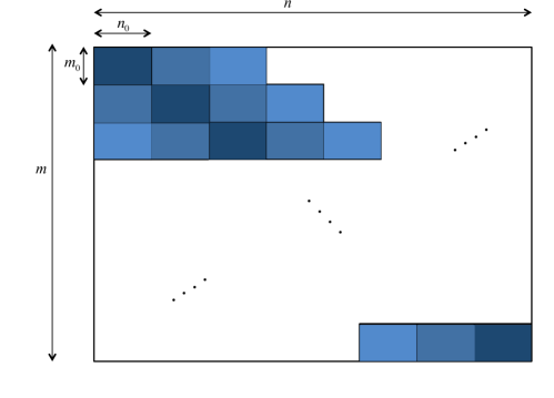
Figure 1: Construction of the spatially coupled measurement matrix $A$ for compressive sensing as described in Section 3.1. The matrix is divided into blocks with size $m_{0}$ by $n_{0}$. (Number of blocks in each row and each column are respectively ${L_{c}}$ and ${L_{r}}$, hence $m=m_{0}{L_{r}}$, $n=n_{0}{L_{c}}$). The matrix elements $A_{ij}$ are chosen as ${\sf N}(0,\frac{1}{m_{0}}W_{{\sf g}(i),{\sf g}(j)})$. In this figure, $W_{i,j}$ depends only on $|i-j|$ and thus blocks on each diagonal have the same variance.

3.2 AMP for compressed sensing reconstruction

AMP algorithms were applied in [DJM11b] to compressed sensing reconstruction with spatially coupled sensing matrices [KMS⁺12b]. Here we follow the scheme and notations of [DJM11b]. In particular, we assume that the unknown vector $x$ to be reconstructed has entries whose empirical distribution converges weakly to a probability measure $p_{X}$ over ${\mathbb{R}}$. The AMP algorithm takes the following form (initialized with $x_{i}^{1}={\mathbb{E}}_{p_{X}}(X)$ for all $i\in[n]$):

$$x^{t+1} = \eta_{t}(x^{t}+(Q^{t}\odot A)^{\sf T}r^{t})\,,$$ (14)

$$r^{t} = y-Ax^{t}+{\sf b}^{t}\odot r^{t-1}\,.$$ (15)

Here, for each $t$, $\eta_{t}:{\mathbb{R}}^{n}\to{\mathbb{R}}^{n}$ is a differentiable non-linear function that depends on the input distribution $p_{X}$. Further, for $v\in{\mathbb{R}}^{n}$, we have $\eta_{t}(v)=(\eta_{t,1}(v_{1}),\dotsc,\eta_{t,n}(v_{n}))$ for some functions $\eta_{i,t}:{\mathbb{R}}\to{\mathbb{R}}$. The symbol $\odot$ indicates Hadamard (entrywise) product. The specific choices for $\eta_{t},Q^{t},{\sf b}^{t}$ are given in Section 3.4 below.

3.3 State evolution

Given $W\in{\mathbb{R}}_{+}^{{\sf R}\times{\sf C}}$ roughly row-stochastic, and undersampling rate $\delta\in(0,1)$, the corresponding state evolution is defined as follows. Start with initial condition

$$\psi_{i}(0)=\infty\mbox{ for all }i\in{\sf C}\,.$$ (16)

For all $t\geq 0$, $a\in{\sf R}$, and $i\in{\sf C}$, let

$$\begin{split}\phi_{a}(t)&=&\sigma^{2}+\frac{1}{\delta}\sum_{i\in{\sf C}}W_{a,i}\,\psi_{i}(t)\,,\\ \psi_{i}(t+1)&=&{\sf mmse}\Big{(}\sum_{b\in{\sf R}}W_{b,i}\phi_{b}(t)^{-1}\Big{)}\,.\end{split}$$ (17)

Here and below, ${\sf mmse}(s)$ denotes the minimum mean square error in estimating $X\sim p_{X}$ from a noisy observation in Gaussian noise, at signal-to-noise ratio $s$. Formally,

$${\sf mmse}(s)={\mathbb{E}}\{[X-{\mathbb{E}}[X|Y]]^{2}\},\quad\quad Y=\sqrt{s}X+Z\,.$$

3.4 Construction of $\eta_{t},{\sf b}^{t},Q^{t}$

In the constructions for the matrix $Q^{t}$, the nonlinearities $\eta_{t}$, and the vector ${\sf b}^{t}$, we use the fact that the state evolution sequence can be precomputed.

Define $Q^{t}$ by

$$Q_{ij}^{t}\equiv\frac{\phi_{{\sf g}(i)}(t)^{-1}}{\sum_{k=1}^{{L_{r}}}W_{k,{\sf g}(j)}\phi_{k}(t)^{-1}}\,.$$ (18)

The nonlinearity $\eta_{t}$ is chosen as follows:

$$\eta_{t}(v)=\big{(}\eta_{t,1}(v_{1}),\eta_{t,2}(v_{2}),\;\dots\;,\eta_{t,N}(v_{N})\big{)}\,,$$ (19)

where $\eta_{t,i}$ is the conditional expectation estimator for $X\sim p_{X}$ in gaussian noise:

$$\eta_{t,i}(v_{i})={\mathbb{E}}\big{\{}X\,\big{|}\,X+\,s_{{\sf g}(i)}(t)^{-1/2}Z=v_{i}\,\big{\}}\,,\;\;\;\;s_{r}(t)\equiv\sum_{u\in{\sf R}}W_{u,r}\phi_{u}(t)^{-1}\,.$$ (20)

Notice that the function $\eta_{t,i}(\,\cdot\,)$ depends on $i$ only through the group index ${\sf g}(i)$, and in fact parametrically through $s_{{\sf g}(i)}(t)$. We define $\tilde{\eta}_{t,i}=\eta_{t,u}$ for $i\in C_{u}$.

Finally, in order to define the vector ${\sf b}^{t}_{i}$, let us introduce the quantity (with $\eta^{\prime}_{t,i}$ denoting the derivative of $v_{i}\mapsto\eta_{t,i}(v_{i})$)

$$\langle\eta^{\prime}_{t}\rangle_{u}=\frac{1}{n_{0}}\sum_{i\in C_{u}}\eta^{\prime}_{t,i}\big{(}x^{t}_{i}+((Q^{t}\odot A)^{\sf T}r^{t})_{i}\big{)}\,.$$ (21)

The vector ${\sf b}^{t}$ is then defined by

$${\sf b}^{t}_{i}\equiv\frac{1}{\delta}\sum_{u\in{\sf C}}W_{{\sf g}(i),u}\widetilde{Q}^{t-1}_{{\sf g}(i),u}\,\langle\eta^{\prime}_{t-1}\rangle_{u}\,,$$ (22)

where we defined $Q^{t}_{i,j}=\widetilde{Q}^{t}_{r,u}$ for $i\in R_{r}$, $j\in C_{u}$.

The following Lemma (Lemma $4.1$ in [DJM11b]) claims that the state evolution (17) allows an exact asymptotic analysis of AMP algorithm (14)- (15) in the limit of a large number of dimensions.

Lemma 1.

Let $W\in{\mathbb{R}}_{+}^{{\sf R}\times{\sf C}}$ be a roughly row-stochastic matrix and $\phi(t)$, $Q^{t}$, ${\sf b}^{t}$ be defined as in Section 3.4. Let $m_{0}=m_{0}(n_{0})$ be such that $m_{0}/n_{0}\to\delta$, as $n_{0}\to\infty$, and let $A(n)\sim{\cal M}(W,m_{0},n_{0})$. Further suppose that the empirical distribution of the entries of $x(n)$ converges weakly to a probability measure $p_{X}$ on ${\mathbb{R}}$ with bounded second moment and the empirical second moment of $x(n)$ also converges to ${\mathbb{E}}_{p_{X}}(X^{2})$. Similarly, suppose that the empirical distribution of the entries of $w(n)$ converges weakly to a probability measure $p_{W}$ on ${\mathbb{R}}$ with bounded second moment and the empirical second moment of $w(n)$ also converges to ${\mathbb{E}}_{p_{W}}(W^{2})\equiv\sigma^{2}$. Then, for all $t\geq 1$, almost surely we have

$$\underset{n_{0}\to\infty}{\rm{lim\,sup}}\frac{1}{n_{0}}\|x^{t}_{C_{a}}(A(n);y(n))-x_{C_{a}}\|_{2}^{2}={\sf mmse}\Big{(}\sum_{i\in{\sf R}}W_{i,a}\phi_{i}(t-1)^{-1}\Big{)}\,,$$ (23)

for all $a\in{\sf C}$, where $x^{t}_{C_{a}},x_{C_{a}}\in{\mathbb{R}}^{n_{0}}$ respectively denote the restrictions of $x^{t},x$ to indices in $C_{a}$.

3.5 Proof of Lemma 1

We show that Lemma 1 follows from Theorem 1. Consider the following change of variables:

$$\tilde{x}^{t+1} = x-(Q^{t}\odot A)^{\sf T}r^{t}-x^{t},$$ (24)

$$\tilde{r}^{t} = w-r^{t}.$$ (25)

Rewriting Eqs (14) and (15) in terms of $\tilde{x}$ and $\tilde{r}$, we obtain

$$\tilde{x}^{t+1} = (Q^{t}\odot A)^{\sf T}(\tilde{r}^{t}-w)-\{\eta_{t-1}(x-\tilde{x}^{t})-x\},$$ (26)

$$\tilde{r}^{t} = A\{\eta_{t-1}(x-\tilde{x}^{t})-x\}+{\sf b}^{t}\odot(\tilde{r}^{t-1}-w).$$ (27)

Let $q={L_{r}}+{L_{c}}$ and define functions $e(\cdot,\cdot,\cdot;t),h(\cdot,\cdot,\cdot;t):{\mathbb{R}}^{q}\times{\mathbb{R}}^{q}\times[q]\to{\mathbb{R}}^{q}$ as follows:

$$h(\mathbf{u},\mathbf{w},a;t) = \sqrt{{L_{r}}}\,(\mathbf{u}(a)-\mathbf{w}(a))\,[\sqrt{W_{a,1}}\widetilde{Q}^{t}_{a,1},\dotsc,\sqrt{W_{a,{L_{c}}}}\widetilde{Q}^{t}_{a,{L_{c}}},\ast,\dotsc,\ast]\quad\;\;\;\text{ for }a\in[{L_{r}}]\,,$$

$$e(\mathbf{v},\mathbf{y},a;t) = \sqrt{{L_{r}}}\,\{\tilde{\eta}_{t-1,a}(\mathbf{y}(a)-\mathbf{v}(a))-\mathbf{y}(a)\}\,[\sqrt{W_{1,a}},\dotsc,\sqrt{W_{{L_{r}},a}},\ast,\dotsc,\ast]\;\;\text{ for }a\in[{L_{c}}]\,.$$

In our definition, we do not care about the values of entries represented by $\ast$, since they are irrelevant for our purposes. Values of $h(\mathbf{u},\mathbf{w},a;t)$ for $a\in\{{L_{r}}+1,\dotsc,{L_{r}}+{L_{c}}\}$ and $e(\mathbf{v},\mathbf{y},a;t)$ for $a\in\{{L_{c}}+1,\dotsc,{L_{r}}+{L_{c}}\}$ are also irrelevant for our purposes and can be defined arbitrarily. Note that $h,e\in\mathrm{PL}(2)$. We also define function $\widehat{e}(\cdot,\cdot;t):{\cal V}_{q,n}\times{\cal V}_{q,n}\to{\cal V}_{q,n}$ by letting $v^{\prime}=\widehat{e}(v,y;t)$ be given by $\mathbf{v}^{\prime}_{j}=e(\mathbf{v}_{j},\mathbf{y}_{j},{\sf g}(j);t)$ for all $j\in[n]$. Similarly, $\widehat{h}(\cdot,\cdot;t):{\cal V}_{q,m}\times{\cal V}_{q,m}\to{\cal V}_{q,m}$ is defined by letting $u^{\prime}=\widehat{h}(u,w;t)$ be given by $\mathbf{u}^{\prime}_{i}=h(\mathbf{u}_{i},\mathbf{w}_{i},{\sf g}(i);t)$ for all $i\in[m]$.

Let $\tilde{A}\in{\mathbb{R}}^{m\times n}$ be a normalized version of $A$ obtained as in the following:

$$\tilde{A}_{ij}=\sqrt{\frac{1}{{L_{r}}\,W_{{\sf g}(i),{\sf g}(j)}}}\,A_{ij}.$$

Therefore, $\tilde{A}$ has i.i.d. entries ${\sf N}(0,1/m)$.

Proposition 5.

Consider the following approximate message passing orbit with vectors $\{v^{t},u^{t}\}_{t\geq 0}$, $v^{t}\in{\cal V}_{q,n}$, $u^{t}\in{\cal V}_{q,m}$:

$$u^{t} = \tilde{A}\,\widehat{e}(v^{t},y;t)-{\sf B}_{t}\,\widehat{h}(u^{t-1},w;t-1)\,,$$ (28)

$$v^{t+1} = \tilde{A}^{{\sf T}}\,\widehat{h}(u^{t},w;t)-{\sf D}_{t}\,\widehat{e}(v^{t},y;t)\,,$$ (29)

for given $y\in{\cal V}_{q,n}$ and $w\in{\cal V}_{q,m}$. Here ${\sf B}_{t}:{\cal V}_{q,m}\to{\cal V}_{q,m}$ is the linear operator defined by letting, for $z^{\prime}={\sf B}_{t}z$, and any $i\in[m]$,

$$\mathbf{z}^{\prime}_{i}=\frac{1}{m}\left(\sum_{k\in[n]}\frac{\partial e}{\partial\mathbf{v}}(\mathbf{v}^{t}_{k},\mathbf{y}_{k},{\sf g}(k);t)\right)\mathbf{z}_{i}\,.$$ (30)

Analogously ${\sf D}_{t}:{\cal V}_{q,n}\to{\cal V}_{q,n}$ is the linear operator defined by letting, for $z^{\prime}={\sf D}_{t}z$, and any $j\in[n]$,

$$\mathbf{z}^{\prime}_{j}=\frac{1}{m}\left(\sum_{l\in[m]}\frac{\partial h}{\partial\mathbf{u}}(\mathbf{u}^{t}_{l},\mathbf{w}_{l},{\sf g}(l);t)\right)\mathbf{z}_{j}\,.$$ (31)

Assume that $y=(\mathbf{y}_{1},\dotsc,\mathbf{y}_{n})$, $w=(\mathbf{w}_{1},\dotsc,\mathbf{w}_{m})$, and $v^{1}=(\mathbf{v}^{1}_{1},\dotsc,\mathbf{v}^{1}_{n})$ are given by

$$\mathbf{y}_{k} =(\ast,\cdots,\ast,\underbrace{x_{k}}_{\rm{position}\,\,{\sf g}(k)},\ast,\cdots,\ast)\in{\mathbb{R}}^{q},\quad\quad\forall k\in[n]$$

$$\mathbf{w}_{k} =(\ast,\cdots,\ast,\underbrace{w_{k}}_{\rm{position}\,\,{\sf g}(k)},\ast,\cdots,\ast)\in{\mathbb{R}}^{q},\quad\quad\forall k\in[m]$$

$$\mathbf{v}^{1}_{k} =(\ast,\cdots,\ast,\underbrace{\tilde{x}^{1}_{k}}_{\rm{position}\,\,{\sf g}(k)},\ast,\cdots,\ast)\in{\mathbb{R}}^{q},\quad\quad\forall k\in[n].$$

Then, we have $\mathbf{u}^{t}_{i}({\sf g}(i))=\tilde{r}^{t}_{i}$ and $\mathbf{v}^{t+1}_{j}({\sf g}(j))=\tilde{x}^{t+1}_{j}$, for all $i\in[m],j\in[n]$, and $t\geq 0$.

We refer to Section 3.5.1 for the proof of Proposition 5.

We proceed by constructing a suitable converging sequence of symmetric AMP instances, recognizing that a subset of the resulting orbit corresponds to the orbit $\{v^{t},u^{t}\}$ of interest. The converging symmetric AMP instances $(A_{s}(N),g,x_{s}^{0})$ are defined as:

• The instances has dimensions $N=m+n$ and $q={L_{r}}+{L_{c}}$.

• Let $B_{1}=C_{1}+C_{1}^{\sf T}$ and $B_{2}=C_{2}+C_{2}^{\sf T}$, where $C_{1}\in{\mathbb{R}}^{m\times m}$ and $C_{2}\in{\mathbb{R}}^{n\times n}$ have i.i.d. entries distributed as ${\sf N}(0,(2m)^{-1})$. The symmetric matrix $A_{s}$ is given by

  $$A_{s}=\sqrt{\frac{\delta}{\delta+1}}\begin{pmatrix}B_{1}&\tilde{A}\\ \tilde{A}^{\sf T}&B_{2}\end{pmatrix}.$$

• Let $\mathbf{y}_{s,i}=\mathbf{w}_{i}\in{\mathbb{R}}^{q}$ for $i\leq m$ and $\mathbf{y}_{s,i}=\mathbf{y}_{i-m}\in{\mathbb{R}}^{q}$ for $i>m$.

• The initial condition is given by $x_{s}^{0}=(\mathbf{x}^{0}_{s,1},\cdots,\mathbf{x}^{0}_{s,N})\in{\cal V}_{q,N}$, where $\mathbf{x}^{0}_{s,i}=0$ for $i\leq m$ and $\mathbf{x}^{0}_{s,i}=\mathbf{v}^{1}_{i-m}$ for $m<i\leq m+n$.

• Finally, for any $\mathbf{x},\mathbf{y}\in{\mathbb{R}}^{q}$, $t\geq 0$, we let

  $$g(\mathbf{x},\mathbf{y},a,2t) = 0\quad\quad\quad\quad\quad\quad\quad\quad\quad\quad\quad\text{for }a\in\{1,\cdots,{L_{r}}\},$$ (32)

  $$g(\mathbf{x},\mathbf{y},a,2t) = \sqrt{\tfrac{\delta+1}{\delta}}\,\,e(\mathbf{x},\mathbf{y},a-{L_{r}};t)\quad\;\text{ for }a\in\{{L_{r}}+1,\cdots,{L_{r}}+{L_{c}}\},$$ (33)

  $$g(\mathbf{x},\mathbf{y},a,2t+1) = \sqrt{\tfrac{\delta+1}{\delta}}\,\,h(\mathbf{x},\mathbf{y},a;t+1)\quad\;\;\;\text{ for }a\in\{1,\cdots,{L_{r}}\},$$ (34)

  $$g(\mathbf{x},\mathbf{y},a,2t+1) = 0\quad\quad\quad\quad\quad\quad\quad\quad\quad\,\quad\quad\text{for }a\in\{{L_{r}}+1,\cdots,{L_{r}}+{L_{c}}\}.$$ (35)

Now, it is easy to see that, for all $t\geq 0$,

$$\mathbf{x}^{2t+1}_{s,i} =\mathbf{u}^{t}_{i},\quad\quad\text{for }i\leq m,$$ (36)

$$\mathbf{x}^{2t}_{s,i} =\mathbf{v}^{t+1}_{i-m},\quad\quad\text{for }m+1\leq i\leq m+n.$$ (37)

Now we are ready to prove Lemma 1 by applying Theorem 1.

Fix $a^{\prime}\in\{{L_{r}}+1,\dotsc,{L_{r}}+{L_{c}}\}$ and $t\geq 1$. Let $a=a^{\prime}-{L_{r}}$ and choose function $\psi(\mathbf{x},\mathbf{y})=\{\tilde{\eta}_{t,a}(\mathbf{y}(a)-\mathbf{x}(a))-\mathbf{y}(a)\}^{2}$. Then,

$$\lim_{n_{0}\to\infty}\frac{1}{n_{0}}\sum_{j^{\prime}\in C_{a^{\prime}}}\psi(\mathbf{x}^{2t}_{s,j},\mathbf{y}_{s,j}) =\lim_{n_{0}\to\infty}\frac{1}{n_{0}}\sum_{j^{\prime}\in C_{a^{\prime}}}[\tilde{\eta}_{t,a}(\mathbf{y}_{s,j^{\prime}}(a)-\mathbf{x}^{2t}_{s,j^{\prime}}(a))-\mathbf{y}_{s,j^{\prime}}(a)]^{2}$$

$$\stackrel{{\scriptstyle(a)}}{{=}}\lim_{n_{0}\to\infty}\frac{1}{n_{0}}\sum_{j\in C_{a}}[\tilde{\eta}_{t,a}(\mathbf{y}_{j}(a)-\mathbf{v}^{t+1}_{j}(a))-\mathbf{y}_{j}(a)]^{2}$$

$$\stackrel{{\scriptstyle(b)}}{{=}}\lim_{n_{0}\to\infty}\frac{1}{n_{0}}\sum_{j\in C_{a}}[\eta_{t,j}(x_{j}-\tilde{x}^{t+1}_{j})-x_{j}]^{2}$$

$$=\lim_{n_{0}\to\infty}\frac{1}{n_{0}}\sum_{j\in C_{a}}(x^{t+1}_{j}-x_{j})^{2}=\lim_{n_{0}\to\infty}\frac{1}{n_{0}}\|x^{t+1}_{C_{a}}-x_{C_{a}}\|^{2}.$$ (38)

Here $(a)$ follows from Eq. (37) and the definition of $\mathbf{y}_{s,j}$ (note that $j^{\prime}=j-m$); $(b)$ follows from the fact $a={\sf g}(j)$ and Proposition 5.

Applying Theorem 1, we have almost surely

$$\lim_{n_{0}\to\infty}\frac{1}{n_{0}}\sum_{j^{\prime}\in C_{a^{\prime}}}\psi(\mathbf{x}^{2t}_{s,j},\mathbf{y}_{s,j})={\mathbb{E}}[\eta_{t,a}(X+Z)-X]^{2},$$ (39)

with $X\sim p_{X}$ and $Z\sim{\sf N}(0,\Sigma^{2t}_{aa})$. Therefore, to complete the proof we need to show that

$$(\Sigma^{2t}_{aa})^{-1}=\sum_{i\in{\sf R}}W_{i,a}\phi_{i}(t)^{-1}.$$ (40)

Note that Eq. (8) reduces to:

$$\Sigma^{t}=\frac{m_{0}}{m+n}\sum_{b^{\prime}=1}^{L_{r}}\widehat{\Sigma}_{b^{\prime}}^{t-1}+\frac{n_{0}}{m+n}\sum_{b^{\prime}={L_{r}}+1}^{{L_{r}}+{L_{c}}}\widehat{\Sigma}_{b^{\prime}}^{t-1}.$$ (41)

By definition of function $g$ (see Eq.s (32)- (35)), it is easy to see that Eq. (9) reduces to:

$$(\widehat{\Sigma}^{2t}_{a^{\prime}})_{ij}=\begin{cases}0,\quad\quad\quad\quad\quad\quad&\text{for }a^{\prime}\in[{L_{r}}],\\ \frac{\delta+1}{\delta}{L_{r}}\sqrt{W_{i,a}W_{j,a}}\,{\mathbb{E}}\{\eta_{t-1,a}(X-Z^{t}_{a})-X\}^{2},&\text{for }a^{\prime}\in\{{L_{r}}+1,\cdots,{L_{r}}+{L_{c}}\},i,j\in[{L_{r}}],\\ *,\quad\quad\quad\quad\quad\quad&\text{otherwise.}\end{cases}$$ (42)

Here $a=a^{\prime}-{L_{r}}$, $X\sim p_{X}$ and $Z_{a}^{t}\sim{\sf N}(0,\Sigma^{2t}_{aa})$. Also,

$$(\widehat{\Sigma}^{2t-1}_{a^{\prime}})_{ij}=\begin{cases}\frac{\delta+1}{\delta}{L_{r}}\sqrt{W_{a^{\prime},i}W_{a^{\prime},j}}\widetilde{Q}^{t}_{a^{\prime},i}\widetilde{Q}^{t}_{a^{\prime},j}\,\{\sigma^{2}+\Sigma^{2t-1}_{a^{\prime}a^{\prime}}\},&\text{for }a^{\prime}\in[{L_{r}}],i,j\in[{L_{c}}],\\ 0,\quad\quad\quad\quad\quad\quad&\text{for }a^{\prime}\in\{{L_{r}}+1,\cdots,{L_{r}}+{L_{c}}\},\\ *,\quad\quad\quad\quad\quad\quad&\text{otherwise.}\end{cases}$$ (43)

Consequently, we obtain

$$\Sigma^{2t}_{aa} =\frac{m_{0}}{m+n}\sum_{b=1}^{{L_{r}}}(\widehat{\Sigma}^{2t-1}_{b})_{aa}$$

$$=\frac{m_{0}{L_{r}}}{m+n}\cdot\frac{\delta+1}{\delta}\sum_{b=1}^{{L_{r}}}W_{b,a}(\widetilde{Q}^{t}_{b,a})^{2}\{\sigma^{2}+\Sigma^{2t-1}_{bb}\}$$

$$=\frac{m_{0}{L_{r}}}{m+n}\cdot\frac{\delta+1}{\delta}\sum_{b=1}^{{L_{r}}}W_{b,a}(\widetilde{Q}^{t}_{b,a})^{2}\{\sigma^{2}+\frac{n_{0}}{m+n}\sum_{c^{\prime}={L_{r}}+1}^{{L_{r}}+{L_{c}}}(\widehat{\Sigma}^{2t-2}_{c^{\prime}})_{bb}\}$$

$$=\frac{m_{0}{L_{r}}}{m+n}\cdot\frac{\delta+1}{\delta}\sum_{b=1}^{{L_{r}}}W_{b,a}(\widetilde{Q}^{t}_{b,a})^{2}\bigg{\{}\sigma^{2}+\frac{n_{0}{L_{r}}}{m+n}\cdot\frac{\delta+1}{\delta}\sum_{c=1}^{{L_{c}}}W_{b,c}{\sf mmse}((\Sigma^{2t-2}_{cc})^{-1})\bigg{\}}$$

$$=\sum_{b=1}^{{L_{r}}}W_{b,a}(\widetilde{Q}^{t}_{b,a})^{2}\bigg{\{}\sigma^{2}+\frac{1}{\delta}\sum_{c=1}^{{L_{c}}}W_{b,c}\,\,{\sf mmse}((\Sigma^{2t-2}_{cc})^{-1})\bigg{\}}.$$

We prove relation (40) using induction on $t$. The induction basis ($t=0$) is trivial. Suppose that the claim holds for $t-1$. Then,

$$\Sigma^{2t}_{aa} =\sum_{b=1}^{{L_{r}}}W_{b,a}(\widetilde{Q}^{t}_{b,a})^{2}\bigg{\{}\sigma^{2}+\frac{1}{\delta}\sum_{c=1}^{{L_{c}}}W_{b,c}\,\,{\sf mmse}(\sum_{i\in{\sf R}}W_{i,c}\phi_{i}(t-1)^{-1})\bigg{\}}$$

$$=\sum_{b=1}^{{L_{r}}}W_{b,a}(\widetilde{Q}^{t}_{b,a})^{2}\phi_{b}(t)$$

$$=\sum_{b=1}^{{L_{r}}}W_{b,a}\frac{\phi_{b}(t)^{-2}}{\left(\sum_{k=1}^{{L_{r}}}W_{k,a}\phi_{k}(t)^{-1}\right)^{2}}\phi_{b}(t)$$

$$=\left(\sum_{b=1}^{{L_{r}}}W_{b,a}\phi_{b}(t)^{-1}\right)^{-1}.$$

This proves the induction claim for $t$. Combining (38),(39) and (40), Lemma 1 follows.

3.5.1 Proof of Proposition 5

We prove the result by induction on $t$. For $t=0$, the claim follows from our definition. Suppose that the claim holds for $t-1$, we prove that for $t$.

Writing Eq. (28) for coordinate $i$, we have

$$\mathbf{u}_{i}^{t}=\sum_{k\in[n]}\tilde{A}_{ik}e(\mathbf{v}^{t}_{k},\mathbf{y}_{k},{\sf g}(k);t)-\frac{1}{m}\left(\sum_{k\in[n]}\frac{\partial e}{\partial\mathbf{v}}(\mathbf{v}_{k}^{t},\mathbf{y}_{k},{\sf g}(k);t)\right)h(\mathbf{u}^{t-1}_{i},\mathbf{w}_{i},{\sf g}(i);t-1)$$ (44)

Restricting to coordinate ${\sf g}(i)$, we get

$$\begin{split}\mathbf{u}_{i}^{t}({\sf g}(i))=&\sum_{k\in[n]}\tilde{A}_{ik}[e(\mathbf{v}^{t}_{k},\mathbf{y}_{k},{\sf g}(k);t)]_{{\sf g}(i)}\\ &-\frac{1}{m}\sum_{k\in[n]}[\frac{\partial e}{\partial v}(\mathbf{v}_{k}^{t}({\sf g}(k)),\mathbf{y}_{k}({\sf g}(k)),{\sf g}(k);t)]_{{\sf g}(i)}\,\,[h(\mathbf{u}^{t-1}_{i},\mathbf{w}_{i},{\sf g}(i);t-1)]_{{\sf g}(k)}.\\ \end{split}$$ (45)

Here, we have used the fact that $e(\mathbf{v}^{t}_{k},\mathbf{y}_{k},{\sf g}(k),t)$ does not depend on $\mathbf{v}^{t}_{k,l}$ for $l\neq{\sf g}(k)$.

Substituting for $e$ and $h$, we have

$$\sum_{k\in[n]}\tilde{A}_{ik}[e(\mathbf{v}^{t}_{k},\mathbf{y}_{k},{\sf g}(k);t)]_{{\sf g}(i)} =\sum_{k\in[n]}\tilde{A}_{ik}\sqrt{{L_{r}}\,W_{{\sf g}(i),{\sf g}(k)}}\{\tilde{\eta}_{t-1,{\sf g}(k)}(\mathbf{y}_{k}({\sf g}(k))-\mathbf{v}^{t}_{k}({\sf g}(k)))-\mathbf{y}_{k}({\sf g}(k))\}$$

$$=\sum_{k\in[n]}A_{ik}\{\eta_{t-1,k}(x_{k}-\tilde{x}^{t}_{k})-x_{k}\},$$ (46)

where we used the induction hypothesis in the last step. Furthermore,

$$\frac{1}{m}\sum_{k\in[n]}[\frac{\partial e}{\partial v}(\mathbf{v}_{k}^{t}({\sf g}(k)),\mathbf{y}_{k}({\sf g}(k)),{\sf g}(k);t)]_{{\sf g}(i)}\,\,[h(\mathbf{u}^{t-1}_{i},\mathbf{w}_{i},{\sf g}(i);t-1)]_{{\sf g}(k)}$$

$$=-\frac{1}{m}\sum_{k\in[n]}\,\tilde{\eta}^{\prime}_{t-1,{\sf g}(k)}\left(\mathbf{y}_{k}({\sf g}(k))-\mathbf{v}^{t}_{k}({\sf g}(k))\right)\sqrt{{L_{r}}\,W_{{\sf g}(i),{\sf g}(k)}}\left(\mathbf{u}^{t-1}_{i}({\sf g}(i))-\mathbf{w}_{i}({\sf g}(i))\right)\sqrt{{L_{r}}\,W_{{\sf g}(i),{\sf g}(k)}}\widetilde{Q}^{t-1}_{{\sf g}(i),{\sf g}(k)}$$

$$=-\frac{1}{m}\sum_{k\in[n]}\,{L_{r}}W_{{\sf g}(i),{\sf g}(k)}\widetilde{Q}^{t-1}_{{\sf g}(i),{\sf g}(k)}\,\eta^{\prime}_{t-1,k}(x_{k}-\tilde{x}^{t}_{k})\,(\tilde{r}^{t-1}_{i}-w_{i})$$

$$=-{\sf b}^{t}_{i}(\tilde{r}^{t-1}_{i}-w_{i}),$$ (47)

where we used the induction hypothesis in the second equality. The last equality follows from the definition of ${\sf b}^{t}_{i}$ (see Eq. (22));

Using (46) and (47) in (45), we obtain

$$\mathbf{u}_{i}^{t}({\sf g}(i))=\sum_{k\in[n]}A_{ik}\{\eta_{t-1,k}(x_{k}-\tilde{x}^{t}_{k})-x_{k}\}+{\sf b}^{t}_{i}(\tilde{r}^{t-1}_{i}-w_{i})=\tilde{r}^{t}_{i},$$ (48)

where the second equality follows from (27). This proves the induction claim for $\mathbf{u}_{i}^{t}({\sf g}(i))$.

Next we prove the claim for $\mathbf{v}^{t+1}_{j}({\sf g}(j))$. Writing Eq. (29) for coordinate $j$, we have

$$\mathbf{v}_{j}^{t+1}=\sum_{l\in[m]}\tilde{A}_{lj}h(\mathbf{u}^{t}_{l},\mathbf{w}_{l},{\sf g}(l);t)-\frac{1}{m}\left(\sum_{l\in[m]}\frac{\partial h}{\partial\mathbf{u}}(\mathbf{u}^{t}_{l},\mathbf{w}_{l},{\sf g}(l);t)\right)e(\mathbf{v}^{t}_{j},\mathbf{y}_{j},{\sf g}(j);t)$$ (49)

Restricting to coordinate ${\sf g}(j)$, we get

$$\begin{split}\mathbf{v}_{j}^{t+1}({\sf g}(j))=&\sum_{l\in[m]}\tilde{A}_{lj}[h(\mathbf{u}^{t}_{l},\mathbf{w}_{l},{\sf g}(l);t)]_{{\sf g}(j)}\\ &-\frac{1}{m}\sum_{l\in[m]}[\frac{\partial h}{\partial u}(\mathbf{u}^{t}_{l}({\sf g}(l)),\mathbf{w}_{l}({\sf g}(l)),{\sf g}(l);t)]_{{\sf g}(j)}[e(\mathbf{v}^{t}_{j},\mathbf{y}_{j},{\sf g}(j);t)]_{{\sf g}(l)}.\end{split}$$ (50)

Here, we have used the fact that $h(\mathbf{u}^{t}_{l},\mathbf{w}_{l},{\sf g}(l),t)$ does not depend on $\mathbf{u}^{t}_{l,k}$ for $k\neq{\sf g}(l)$.

Substituting for $e$ and $h$, we have

$$\sum_{l\in[m]}\tilde{A}_{lj}[h(\mathbf{u}^{t}_{l},\mathbf{w}_{l},{\sf g}(l);t)]_{{\sf g}(j)} =\sum_{l\in[m]}\tilde{A}_{lj}\sqrt{{L_{r}}\,W_{{\sf g}(l),{\sf g}(j)}}\,\widetilde{Q}^{t}_{{\sf g}(l),{\sf g}(j)}\,(\mathbf{u}^{t}_{l}({\sf g}(l))-\mathbf{w}_{l}({\sf g}(l)))$$

$$=\sum_{l\in[m]}A_{lj}Q^{t}_{l,j}\,(\tilde{r}^{t}_{l}-w_{l}),$$ (51)

where in the last step we used the result $\mathbf{u}^{t}_{l}({\sf g}(l))=\tilde{r}^{t}_{l}$, proved above. Moreover,

$$\frac{1}{m}\sum_{l\in[m]}[\frac{\partial h}{\partial u}(\mathbf{u}^{t}_{l}({\sf g}(l)),\mathbf{w}_{l}({\sf g}(l)),{\sf g}(l);t)]_{{\sf g}(j)}[e(\mathbf{v}^{t}_{j},\mathbf{y}_{j},{\sf g}(j);t)]_{{\sf g}(l)}$$

$$=\frac{1}{m}\sum_{l\in[m]}\sqrt{{L_{r}}W_{{\sf g}(l),{\sf g}(j)}}\,\widetilde{Q}^{t}_{{\sf g}(l),{\sf g}(j)}\{\tilde{\eta}_{t-1,{\sf g}(j)}(\mathbf{y}_{j}({\sf g}(j))-\mathbf{v}^{t}_{j}({\sf g}(j)))-\mathbf{y}_{j}({\sf g}(j))\}\,\sqrt{{L_{r}}W_{{\sf g}(l),{\sf g}(j)}}$$

$$=\frac{1}{m}\left(\sum_{l\in[m]}{L_{r}}W_{{\sf g}(l),{\sf g}(j)}Q^{t}_{l,j}\right)\{\eta_{t-1,j}(x_{j}-\tilde{x}^{t}_{j})-x_{j}\}$$

$$=\eta_{t-1,j}(x_{j}-\tilde{x}^{t}_{j})-x_{j}.$$ (52)

Using (51) and (52) in (50), we obtain

$$\mathbf{v}^{t+1}_{j}({\sf g}(j))=\sum_{l\in[m]}A_{lj}Q^{t}_{l,j}\,(\tilde{r}^{t}_{l}-w_{l})-\{\eta_{t-1,j}(x_{j}-\tilde{x}^{t}_{j})-x_{j}\}=\tilde{x}^{t+1}_{j},$$ (53)

where the second equality follows from (26). This proves the induction claim for $\mathbf{v}_{i}^{t+1}({\sf g}(i))$.

4 Proof of Theorem 1

4.1 Definitions and notations

Letting $m^{t}=f(x^{t};t)$ for $t\geq 0$, Eq. (5), becomes

$$x^{t+1}=A\,m^{t}-{\sf B}_{t}\,m^{t-1}\,.$$ (54)

This is initialized with $m^{-1}=0$ and $m^{0}=m^{0,N}\in{\cal V}_{q,N}$, a sequence of deterministic vectors in ${\cal V}_{q,N}$, with $\lim\sup_{N\to\infty}N^{-1}\sum_{i=1}^{N}\|\mathbf{m}^{0}_{i}\|^{2k-2}<\infty$. Also recall that the vectors $y=(\mathbf{y}_{1},\dotsc,\mathbf{y}_{N})\in{\cal V}_{q,N}$ are a fixed sequence indexed by $N$, with converging empirical distributions.

The idea of the proof is to study the stochastic process $\{x^{0},x^{1},\dots,x^{t},\dots\}$ taking values in ${\cal V}_{q,N}$ without conditioning on the matrix $A$. Instead, for each $t$, we will compute the conditional distribution of $x^{t+1}$ given $x^{0},\ldots,x^{t}$, and hence $m^{0},\ldots,m^{t}$. More precisely, let $\mathfrak{S}_{t}$ be the $\sigma$-algebra generated by these variables. We will compute the conditional distributions $x^{t+1}|_{\mathfrak{S}_{t}}$, by characterizing the conditional distribution of the matrix $A$ given this filtration.

Throughout the proof, we identify ${\cal V}_{q,N}$ with the set of matrices ${\mathbb{R}}^{N\times q}$. Adopting this convention, the linear operator ${\sf B}_{t}$ can be more conveniently identified with the $q\times q$ matrix

$${\bf B}_{t}=\frac{1}{N}\left(\sum_{j\in[N]}\frac{\partial f^{j}}{\partial\mathbf{x}}(\mathbf{x}^{t}_{j},t)\right)\,.$$ (55)

We therefore have ${\sf B}_{t}m_{t-1}=m_{t-1}{\bf B}_{t}^{{\sf T}}$ and the equations for $x^{1},\ldots,x^{t}$ can be written in matrix form as:

$$\underbrace{\left[x^{1}|x^{2}+m^{0}{\bf B}_{1}^{{\sf T}}|\ldots|x^{t}+m^{t-2}{\bf B}_{t-1}^{{\sf T}}\right]}_{Y_{t-1}} =A\underbrace{[m^{0}|\ldots|m^{t-1}]}_{M_{t-1}}.$$ (56)

In short $Y_{t-1}=AM_{t-1}$. Here and below we use $[Q|P]$ to denote the matrix obtained by concatenating $Q$ and $P$ horizontally.

We also introduce the notation $m_{\parallel}^{t}$ for the projection of $m^{t}$ onto the column space of $M_{t-1}$. More precisely, $m_{\parallel}^{t}\in{\mathbb{R}}^{N\times q}$ is the matrix whose columns are the projections of the columns of $m^{t}$. This can be written as

$$m_{\parallel}^{t}=\sum_{i=0}^{t-1}m^{i}\alpha_{i}\,,$$ (57)

where $\alpha_{i}\in{\mathbb{R}}^{q\times q}$, $0\leq i\leq t-1$ contain the coefficients of these projections. Defining by $m_{\perp}^{t}=m^{t}-m_{\parallel}^{t}$ the perpendicular component , we have $M_{t-1}^{{\sf T}}m_{\perp}^{t}=0$. We further denote by $\alpha\in{\mathbb{R}}^{tq\times q}$ the matrix obtained by concatenating $\alpha_{i}$’s vertically. Using this notation, we have

$$m_{\parallel}^{t}=M_{t-1}\alpha\,.$$ (58)

For an integer $\ell\geq 1$, let $(\ell)=\{(\ell-1)q+1,\dotsc,\ell q\}$. For a matrix $u$ and set of indices $I,J$, we let $u_{I,J}$ denote the submatrix formed by the rows in $I$ and columns in $J$. We further let $u_{I}$ denote the submatrix containing just the rows in $I$. For $v=(\mathbf{v}_{1},\dotsc,\mathbf{v}_{N})\in{\cal V}_{q,N}$ and a set of indices $I=\{i_{1},\dotsc,i_{r}\}$, let $v_{I}=(\mathbf{v}_{i_{1}},\dotsc,\mathbf{v}_{i_{r}})$.

Given $v\in{\cal V}_{q,m}$ and $\varphi:{\mathbb{R}}^{q}\to{\mathbb{R}}^{q}$, we write $\varphi(v)=(\varphi(\mathbf{v}_{1}),\dotsc,\varphi(\mathbf{v}_{m}))$. We also define $\nabla\varphi(v)=[\frac{\partial\varphi}{\partial\mathbf{v}}(\mathbf{v}_{1}),\dotsc,\frac{\partial\varphi}{\partial\mathbf{v}}(\mathbf{v}_{m})]^{\sf T}$ with $\frac{\partial\varphi}{\partial\mathbf{v}}\in{\mathbb{R}}^{q\times q}$ denoting the Jacobian matrix of $\varphi$. Note that $\nabla\varphi(v)\in{\mathbb{R}}^{mq\times q}$.

For $u\in{\mathbb{R}}^{mq\times q}$, let $\langle u\rangle=(1/m)\sum_{i=1}^{m}u_{(i)}\in{\mathbb{R}}^{q\times q}$. Also, for $u,v\in{\cal V}_{q,N}$ we define

$$\langle u,v\rangle=\frac{1}{N}\sum_{i=1}^{N}\mathbf{u}_{i}\mathbf{v}_{i}^{\sf T}\in{\mathbb{R}}^{q\times q}.$$

Note that $\langle u,v\rangle=(1/N)u^{\sf T}v$, as we regard ${\cal V}_{q,N}\equiv{\mathbb{R}}^{N\times q}$.

Given two random variables $X,Y$, and a $\sigma$-algebra $\mathfrak{S}$, the notation $X|_{\mathfrak{S}}\stackrel{{\scriptstyle\text{\rm d}}}{{=}}Y$ means that for any integrable function $\phi$ and for any random variable $Z$ measurable on $\mathfrak{S}$, ${\mathbb{E}}\{\phi(X)Z\}={\mathbb{E}}\{\phi(Y)Z\}$. In words we will say that $X$ is distributed as (or is equal in distribution to) $Y$ conditional on $\mathfrak{S}$. In case $\mathfrak{S}$ is the trivial $\sigma$-algebra we simply write $X\stackrel{{\scriptstyle\text{\rm d}}}{{=}}Y$ (i.e. $X$ and $Y$ are equal in distribution). For random variables $X,Y$ the notation $X\stackrel{{\scriptstyle{\rm a.s.}}}{{=}}Y$ means that $X$ and $Y$ are equal almost surely.

The large system limit will be denoted as $\lim_{N\to\infty}$. In the large system limit, we use the notation $\vec{o}_{t}(1)$ to represent a matrix in ${\mathbb{R}}^{tq\times q}$ (with $t$ fixed) such that all of its coordinates converge to 0 almost surely as $N\to\infty$.

The indicator function of property ${\cal A}$ is denoted by $\mathbb{I}({\cal A})$ or $\mathbb{I}_{{\cal A}}$. The normal distribution with mean $\mu$ and variance $v^{2}$ is represented as ${\sf N}(\mu,v^{2})$.

4.2 Main technical Lemma

We will say that a convergent sequence of mappings $({\cal F}_{N})_{N\in{\mathbb{N}}}$ is non-trivial if there exists ${\varepsilon}_{0}>0$ such that, for each $N$, $t\geq 0$, $a\in[q]$, $i\in[N]$, $\mathbf{\gamma}\in{\mathbb{R}}^{q}$ with $\|\mathbf{\gamma}\|_{2}=1$, $b\in{\mathbb{R}}$, we have

$$\int\big{(}\gamma^{\sf T}g(\mathbf{x},\mathbf{y}_{i},a,t)-b\big{)}^{2}{\rm d}\mathbf{x}\geq{\varepsilon}_{0}\,.$$

This condition is useful to rule out trivial degeneracies.

Lemma 2.

Let $\{(A(N),{\cal F}_{N},x^{0,N})\}_{N}$ be a converging sequence of AMP instances as in Theorem 1 with ${\cal F}_{N}$ non-trivial. Then the following hold for all $t\in{\mathbb{N}}$

• $$x^{t+1}|_{\mathfrak{S}_{t}} \stackrel{{\scriptstyle\text{\rm d}}}{{=}}\sum_{i=0}^{t-1}x^{i+1}{\alpha_{i}}+{\tilde{A}}m_{\perp}^{t}+\tilde{M}_{t-1}\vec{o}_{t-1}(1)\,,$$ (59)

  where ${\tilde{A}}$ is an independent copy of $A$. The matrix $\tilde{M}_{t}$ is such that its columns form an orthogonal basis for the column space of $M_{t}$ and $\tilde{M}_{t}^{\sf T}\tilde{M}_{t}=N\,{\rm I}_{tq\times tq}$. Recall that, $\vec{o}_{t-1}(1)\in{\mathbb{R}}^{(t-1)q\times q}$ is a random vector that converges to 0 almost surely as $N\to\infty$.

• For any pseudo-Lipschitz function $\phi:({\mathbb{R}}^{q})^{t+2}\to{\mathbb{R}}$ of order $k$,

  $$\lim_{N\to\infty}\frac{1}{|C_{a}^{N}|}\sum_{i\in C_{a}^{N}}\phi(\mathbf{x}_{i}^{1},\ldots,\mathbf{x}_{i}^{t+1},\mathbf{y}_{i}) \stackrel{{\scriptstyle{\rm a.s.}}}{{=}}{\mathbb{E}}\big{[}\phi(Z_{a}^{1},\ldots,Z_{a}^{t+1},Y_{a})\big{]}\,.$$ (60)

  where $(Z_{a}^{1},\dots,Z_{a}^{t+1})$ is a Gaussian vector independent of $Y_{a}\sim P_{a}$ and, for each $i$, $Z_{a}^{i}\sim{\sf N}(0,\Sigma^{i})$

• For all $1\leq r,s\leq t,a\in[q]$ the following equations hold and all limits exist, are bounded and have degenerate distribution (i.e. they are constant random variables):

  $$\lim_{N\to\infty}\langle x_{C^{N}_{a}}^{r+1},x_{C^{N}_{a}}^{s+1}\rangle \stackrel{{\scriptstyle{\rm a.s.}}}{{=}}\lim_{N\to\infty}\langle m^{r},m^{s}\rangle\,.$$ (61)

• Consider any set of $q$ Lipschitz continuous functions $\varphi^{a}:{\mathbb{R}}^{q}\times{\mathbb{R}}^{q}\to{\mathbb{R}}^{q}$. For all $1\leq r,s\leq t$, the following equations hold and all limits exist, are bounded and have degenerate distribution (i.e. they are constant random matrices):

  $$\lim_{N\to\infty}\langle x^{r+1}_{C^{N}_{a}},\varphi(x^{s+1}_{C^{N}_{a}},y_{C^{N}_{a}})\rangle \stackrel{{\scriptstyle{\rm a.s.}}}{{=}}\lim_{N\to\infty}\langle x^{r+1}_{C^{N}_{a}},x^{s+1}_{C^{N}_{a}}\rangle\langle\nabla\varphi^{a}(x^{s+1}_{C^{N}_{a}},y_{C^{N}_{a}})\rangle\,.$$ (62)

  The Jacobians here are computed according to the first component. Define $\varphi:{\cal V}_{q,N}\times{\cal V}_{q,N}\to{\cal V}_{q,N}$ by letting $v^{\prime}=\varphi(u,v)$ be given by $\mathbf{v}^{\prime}_{i}=\varphi^{a}(\mathbf{u}_{i},\mathbf{v}_{i})$ for $i\in C^{N}_{a}$. Let $\nabla\varphi\in{\mathbb{R}}^{Nq\times q}$ be the matrix obtained by concatenating the matrices $\nabla\varphi^{a}\in{\mathbb{R}}^{|C^{N}_{a}|q\times q}$, for $a\in[q]$. Then, Eq. (62) implies that for all $1\leq r,s\leq t$, the following equations hold:

  $$\lim_{N\to\infty}\langle x^{r+1},\varphi(x^{s+1},y)\rangle \stackrel{{\scriptstyle{\rm a.s.}}}{{=}}\lim_{N\to\infty}\langle x^{r+1},x^{s+1}\rangle\langle\nabla\varphi(x^{s+1},y)\rangle\,.$$ (63)

• For $\ell=k-1$ and $a\in[q]$, the following holds almost surely

  $$\lim_{N\to\infty}\frac{1}{|C^{N}_{a}|}\sum_{i\in C^{N}_{a}}\|\mathbf{x}_{i}^{t+1}\|^{2\ell}<\infty\,.$$ (64)

• For all $0\leq r\leq t$ the following limit exists and there are positive constants $\rho_{r}$ (independent of $N$) such that almost surely

  $$\lim_{N\to\infty}\langle m_{\perp}^{r},m_{\perp}^{r}\rangle-\rho_{r}\,{\rm I}_{q\times q}\succeq 0\,.$$ (65)

4.2.1 Proof of Theorem 1

First assume that the sequence of functions ${\cal F}_{N}$ is non-trivial. Theorem 1 follows readily from Lemma 2. More specifically, Theorem 1 is obtained by applying Lemma 2$(b)$ to functions $\phi(\mathbf{x}^{1}_{i},\dotsc,\mathbf{x}^{t}_{i})=\psi(\mathbf{x}^{t}_{i},\mathbf{y}_{i})$.

Consider then the case in which ${\cal F}_{N}$ is not non-trivial. In this case we perturb the functions $g(\mathbf{x},\mathbf{y},a,t)$ as follows. Let $\varphi(\mathbf{x}):{\mathbb{R}}^{q}\to{\mathbb{R}}^{q}$ be a bounded smooth function. Define

$$g^{\epsilon}(\mathbf{x},\mathbf{y},a,t)=g(\mathbf{x},\mathbf{y},a,t)+\epsilon\,\varphi(\mathbf{x}).$$

The resulting sequence of instances is then non-trivial and state evolution applies. Call $\Sigma^{t}({\varepsilon})$ the resulting state evolution sequence, and denote by $x^{t}(\epsilon)$ the corresponding orbit. Applying Theorem 1, we have

$$\lim_{N\to\infty}\frac{1}{N}\sum_{i=1}^{N}\psi(\mathbf{x}^{t}_{j}(\epsilon),\mathbf{y}_{i})={\mathbb{E}}\{\psi(Z^{t}_{a}(\epsilon),Y_{a})\},$$ (66)

with $Z^{t}_{a}(\epsilon)\sim{\sf N}(0,\Sigma^{t}(\epsilon))$. In order to prove the same theorem for the orbit $\{x^{t}\}_{t\geq 0}$, we need to show the following two facts:

• $\lim_{\epsilon\to 0}{\mathbb{E}}\{\psi(Z^{t}_{a}(\epsilon),Y_{a})\}={\mathbb{E}}\{\psi(Z^{t}_{a},Y_{a})\}$, with $Z^{t}_{a}\sim{\sf N}(0,\Sigma^{t})$.

• Let $a_{N}(\epsilon)=\frac{1}{N}\sum_{i=1}^{N}\psi(\mathbf{x}^{t}_{i}(\epsilon),\mathbf{y}_{i})$. Then $|a_{N}(\epsilon)-a_{N}(0)|\leq C\epsilon$, with constant $C$ being independent of $N$.

Given $(i)$-$(ii)$, we have

$$\lim_{N\to\infty}\big{|}a_{N}(0)-{\mathbb{E}}\{\psi(Z^{t}_{a},Y_{a})\}\big{|}\leq{\rm{lim\,sup}}_{N\to\infty}\Big{\{} \big{|}a_{N}(0)-a_{N}(\epsilon)\big{|}+\big{|}a_{N}(\epsilon)-{\mathbb{E}}\{\psi(Z^{t}_{a}(\epsilon),Y_{a})\}\big{|}\Big{\}}$$

$$+ \big{|}{\mathbb{E}}\{\psi(Z^{t}_{a}(\epsilon),Y_{a})\}-{\mathbb{E}}\{\psi(Z^{t}_{a},Y_{a})\}\big{|}$$

$$\leq C\varepsilon+0+\big{|}{\mathbb{E}}\{\psi(Z^{t}_{a}(\epsilon),Y_{a})\}-{\mathbb{E}}\{\psi(Z^{t}_{a},Y_{a})\}\big{|},$$

where the last step follows from $(ii)$ and Eq. (66). Therefore, taking the limit of both sides as $\epsilon\to 0$,

$$\lim_{N\to\infty}\big{|}a_{N}(0)-{\mathbb{E}}\{\psi(Z^{t}_{a},Y_{a})\}\big{|} \leq\lim_{\epsilon\to 0}C\varepsilon+\lim_{\epsilon\to 0}\big{|}{\mathbb{E}}\{\psi(Z^{t}_{a}(\epsilon),Y_{a})\}-{\mathbb{E}}\{\psi(Z^{t}_{a},Y_{a})\}\big{|}=0\,,$$

where the last step follows from $(i)$. This proves Theorem 1 for $\{x^{t}\}_{t\geq 0}$.

It remains to prove facts $(i)$-$(ii)$. The claim in $(i)$ follows readily by applying dominated convergence theorem and noting that $\psi(\cdot,\cdot)$ is Lipschitz continuous.

To prove $(ii)$, write

$$|a_{N}(\epsilon)-a_{N}(0)|$$

$$\leq\frac{1}{N}\sum_{i=1}^{N}\big{|}\psi(\mathbf{x}^{t}_{i}(\epsilon),\mathbf{y}_{i})-\psi(\mathbf{x}^{t}_{i},\mathbf{y}_{i})\big{|}$$

$$\leq\frac{L^{\prime}}{N}\,\sum_{i=1}^{N}(1+\|\mathbf{x}^{t}_{i}(\epsilon)\|^{k-1}+\|\mathbf{x}^{t}_{i}\|^{k-1}+\|\mathbf{y}_{i}\|^{k-1})\,\|\mathbf{x}^{t}_{i}(\epsilon)-\mathbf{x}^{t}_{i}\|$$

$$\leq\frac{L^{\prime}}{N}\,\Big{\{}\sum_{i=1}^{N}(1+\|\mathbf{x}^{t}_{i}(\epsilon)\|^{k-1}+\|\mathbf{x}^{t}_{i}\|^{k-1}+\|\mathbf{y}_{i}\|^{k-1})^{2}\Big{\}}^{\frac{1}{2}}\Big{\{}\sum_{i=1}^{N}\|\mathbf{x}^{t}_{i}(\epsilon)-\mathbf{x}^{t}_{i}\|^{2}\Big{\}}^{\frac{1}{2}}$$

$$\leq{3L^{\prime}}\,\Big{\{}1+\frac{1}{N}\sum_{i=1}^{N}\|\mathbf{x}^{t}_{i}(\epsilon)\|^{2k-2}+\frac{1}{N}\sum_{i=1}^{N}\|\mathbf{x}^{t}_{i}\|^{2k-2}+\frac{1}{N}\sum_{i=1}^{N}\|\mathbf{y}_{i}\|^{2k-2}\Big{\}}^{\frac{1}{2}}\Big{\{}\frac{1}{N}\sum_{i=1}^{N}\|\mathbf{x}^{t}_{i}(\epsilon)-\mathbf{x}^{t}_{i}\|^{2}\Big{\}}^{\frac{1}{2}}\,,$$

where second inequality holds since $\psi\in\mathrm{PL}(k)$ and third inequality follows by using Cauchy-Schwartz inequality. In the last expression, the term in the first braces is bounded using the assumption on the second moment of $y$ and using part $(e)$ of Lemma 2 for orbit $\{x^{t}(\epsilon)\}$. To bound the second braces, note that both $A$ and ${\sf B}_{t}$ in the AMP iteration (5) have bounded operator norm (the former with probability $1-e^{-\Theta(N)}$). Since $g(\,\cdot\,,t)$ is Lipschitz continuous and $\varphi(\mathbf{x})$ is bounded by assumption, we conclude that $\|x^{t}({\varepsilon})-x^{t}\|^{2}\leq c^{t}N{\varepsilon}^{2}$ for some absolute constant $c$. This completes the proof of fact $(ii)$.

4.3 Proof of Lemma 2

The proof is by induction on $t$. Let $\mathcal{B}_{t}$ be the property that (59), (60), (61), (63), (64), and (65) hold.

4.3.1 Induction basis: $\mathcal{B}_{0}$

Note that $x^{1}=Am^{0}$.

• $\mathfrak{S}_{0}$ is generated by $y$, $x^{0}$ and $m^{0}$. Also $m^{0}=m^{0}_{\perp}$ since $M_{-1}$ is an empty matrix. Hence

  $$x^{1}|_{\mathfrak{S}_{1}}=Am^{0}_{\perp}.$$

• Let $\phi:{\cal V}_{q,2}\to{\mathbb{R}}$ be a pseudo-Lipschitz function of order $k$. Hence, $|\phi(x)|\leq L(1+\|x\|^{k})$. Given $m^{0}$, $y$, the random variable $\sum_{i\in C^{N}_{a}}\phi([Am^{0}]_{i},\mathbf{y}_{i})/|C^{N}_{a}|$ is a sum of independent random variables. By Lemma 4(a) $[Am^{0}]_{i}\stackrel{{\scriptstyle\text{\rm d}}}{{=}}Z$ for $Z\sim{\sf N}(0,\langle m^{0},m^{0}\rangle)$. Using Eq. (7),

  $$\lim_{N\to\infty}\langle m^{0},m^{0}\rangle =\sum_{a\in[q]}c_{a}\left(\lim_{N\to\infty}\frac{1}{|C_{a}^{N}|}\sum_{i\in C^{N}_{a}}(\mathbf{m}^{0}_{i})^{\sf T}\mathbf{m}^{0}_{i}\right)$$

  $$=\sum_{a\in[q]}c_{a}\widehat{\Sigma}^{0}_{a}=\Sigma^{1}.$$

  Hence for all $p\geq 1$, there exists a constant $c_{p}$ such that ${\mathbb{E}}\{\|[Am^{0}]_{i}\|^{p}\}\leq\|\langle m^{0}_{\perp},m^{0}_{\perp}\rangle\|_{2}^{\frac{p}{2}}\;{\mathbb{E}}_{Z}\|Z\|^{p}<c_{p}$, with $Z\sim{\sf N}(0,{\rm I}_{q})$. Next, we check conditions of Theorem 2 for $X_{N,i}\equiv\phi(\mathbf{x}_{i}^{1},\mathbf{y}_{i})-{\mathbb{E}}_{A}\{\phi(\mathbf{x}_{i}^{1},\mathbf{y}_{i})\}$ for $\kappa>0$,

  $$\frac{1}{|C_{a}^{N}|}\sum_{i\in C^{N}_{a}}{\mathbb{E}}|X_{N,i}|^{2+\kappa}$$ (67)

  $$=\frac{1}{|C_{a}^{N}|}\sum_{i\in C^{N}_{a}}{\mathbb{E}}\big{|}\phi(\mathbf{x}_{i}^{1},\mathbf{y}_{i})-{\mathbb{E}}_{A}\{\phi(\mathbf{x}_{i}^{1},\mathbf{y}_{i})\}\big{|}^{2+\kappa}$$

  $$=\frac{1}{|C_{a}^{N}|}\sum_{i\in C^{N}_{a}}\left|{\mathbb{E}}_{A,\tilde{A}}\left\{\phi([\tilde{A}m^{0}]_{i},\mathbf{y}_{i})-\phi([Am^{0}]_{i},\mathbf{y}_{i})\right\}\right|^{2+\kappa}$$

  $$\leq\frac{1}{|C_{a}^{N}|}\sum_{i\in C^{N}_{a}}\left|{\mathbb{E}}_{A,\tilde{A}}\left\{\phi([\tilde{A}m^{0}]_{i},\mathbf{y}_{i})-\phi([Am^{0}]_{i},\mathbf{y}_{i})\right\}\right|^{2+\kappa}$$

  $$\leq\frac{1}{|C_{a}^{N}|}\sum_{i\in C^{N}_{a}}\left|{\mathbb{E}}_{A,\tilde{A}}\left\{\|[\tilde{A}m^{0}]_{i}-[Am^{0}]_{i}\|(1+\|\mathbf{y}_{i}\|^{k-1}+\|[\tilde{A}m^{0}]_{i}\|^{k-1}+\|[Am^{0}]_{i}\|^{k-1})\right\}\right|^{2+\kappa}$$

  $$\leq c+\frac{L^{\prime}c^{\prime}}{|C^{N}_{a}|}\sum_{i\in C^{N}_{a}}\|\mathbf{y}_{i}\|^{(k-1)(2+\kappa)}$$

  $$\leq c+L^{\prime}c^{\prime}|C^{N}_{a}|^{\kappa/2}\left(\frac{1}{|C_{a}^{N}|}\sum_{i\in C^{N}_{a}}\|\mathbf{y}_{i}\|^{2(k-1)}\right)^{1+\kappa/2}\leq c^{\prime\prime}|C_{a}^{N}|^{\kappa/2}.$$

  Here $\tilde{A}$ is an independent copy of $A$, and the last inequality uses assumption on empirical moments of $\{\mathbf{y}_{i}\}_{i\in C^{N}_{a}}$. By applying Theorem 2, we get

  $$\lim_{N\to\infty}\frac{1}{|C_{a}^{N}|}\sum_{i\in C^{N}_{a}}\left[\phi(\mathbf{x}_{i}^{1},\mathbf{y}_{i})-{\mathbb{E}}_{A}\{\phi(\mathbf{x}_{i}^{1},\mathbf{y}_{i})\}\right]\stackrel{{\scriptstyle{\rm a.s.}}}{{=}}0.$$

  Hence, using Lemma 6 for $v=w$ and $\psi(\mathbf{y}_{i})={\mathbb{E}}_{Z}\{\phi(Z,\mathbf{y}_{i})\}$ we get

  $$\lim_{N\to\infty}\frac{1}{C^{N}_{a}}\sum_{i\in C^{N}_{a}}{\mathbb{E}}_{Z}[\phi(\mathbf{x}^{1}_{i},\mathbf{y}_{i})]\stackrel{{\scriptstyle{\rm a.s.}}}{{=}}{\mathbb{E}}\big{\{}\phi(Z_{a},Y_{a})\big{\}},$$

  with $Z_{a}\sim{\sf N}(0,\Sigma^{1})$ independent of $Y_{a}\sim P_{a}$. Note that $\psi$ belongs to $\mathrm{PL}(k)$ since $\phi$ belongs to $\mathrm{PL}(k)$.

• Let $\hat{A}=A_{C^{N}_{a}}$ be the submatrix formed by the rows in $C^{N}_{A}$. Using Lemma 4(c), conditioned on $m^{0}$,

  $$\lim_{N\to\infty}\langle x_{C^{N}_{a}}^{1},x_{C^{N}_{a}}^{1}\rangle=\lim_{N\to\infty}\langle\hat{A}m^{0},\hat{A}m^{0}\rangle\stackrel{{\scriptstyle{\rm a.s.}}}{{=}}\lim_{N\to\infty}\langle m^{0},m^{0}\rangle=\Sigma^{1}\,.$$

• Write

  $$\lim_{N\to\infty}\langle x^{1}_{C^{N}_{a}},\varphi(x^{1}_{C^{N}_{a}},y_{C^{N}_{a}})\rangle=\lim_{N\to\infty}\frac{1}{|C^{N}_{a}|}\sum_{i\in C^{N}_{a}}\mathbf{x}^{1}_{i}[\varphi^{a}(\mathbf{x}^{1}_{i},\mathbf{y}_{i})]^{\sf T}\stackrel{{\scriptstyle{\rm a.s.}}}{{=}}{\mathbb{E}}(Z_{a}[\varphi^{a}(Z_{a},Y_{a})]^{\sf T}),$$

  where the last step follows by applying $\mathcal{B}_{0}(b)$ to the functions $\phi(\mathbf{x}^{1}_{i},\mathbf{y}_{i})=\mathbf{x}^{1}_{i}(l)[\varphi^{a}(\mathbf{x}_{i}^{1},\mathbf{y}_{i})]_{k}$, for all $l,k\in[q]$. Furthermore, using Lemma 5,

  $${\mathbb{E}}(Z_{a}[\varphi^{a}(Z_{a},Y_{a})]^{\sf T})=\Sigma^{1}\,{\mathbb{E}}([\frac{\partial\varphi^{a}}{\partial\mathbf{z}}(Z_{a},Y_{a})]^{\sf T})\,.$$

  As proved in part $(c)$, $\lim_{N\to\infty}\langle x^{1}_{C^{N}_{a}},x^{1}_{C^{N}_{a}}\rangle=\Sigma^{1}$. Also, by part $(b)$, the empirical distribution of $\{(\mathbf{x}_{i}^{1},\mathbf{y}_{i})\}_{i\in C^{N}_{a}}$ converges weakly to the distribution of $(Z_{a},Y_{a})$, and consequently we get

  $$\lim_{N\to\infty}\langle\nabla\varphi^{a}(x^{1}_{C^{N}_{a}},y_{C^{N}_{a}})\rangle=\lim_{N\to\infty}\frac{1}{|C^{N}_{a}|}\sum_{i\in C^{N}_{a}}[\frac{\partial\varphi^{a}}{\partial\mathbf{x}}(\mathbf{x}_{i}^{1},\mathbf{y}_{i})]^{\sf T}\stackrel{{\scriptstyle{\rm a.s.}}}{{=}}{\mathbb{E}}([\frac{\partial\varphi^{a}}{\partial\mathbf{z}}(Z_{a},Y_{a})]^{\sf T})\,.$$

  This proves Eq. (62). To prove Eq. (63), notice that

  $$\langle x^{1},\varphi(x^{1},y)\rangle=\sum_{a\in[q]}c_{a}\langle x^{1}_{C^{N}_{a}},\varphi(x^{1}_{C^{N}_{a}},y_{C^{N}_{a}})\rangle\,.$$ (68)

  Also,

  $$\lim_{N\to\infty}\langle x^{1},x^{1}\rangle=\sum_{a\in[q]}c_{a}\lim_{N\to\infty}\langle x^{1}_{C^{N}_{a}},x^{1}_{C^{N}_{a}}\rangle=\sum_{a\in[q]}c_{a}\Sigma^{1}=\Sigma^{1},$$ (69)

  where the last step holds since $\sum_{a\in[q]}c_{a}=1$. Further,

  $$\langle\nabla\varphi(x^{1},y)\rangle=\sum_{a\in[q]}c_{a}\langle\nabla\varphi^{a}(x^{1}_{C^{N}_{a}},y_{C^{N}_{a}})\rangle$$ (70)

  Combining Eqs. (68),  (69), (70) and Eq. (62), we get the desired result.

• Similar to $(b)$, conditioning on $m^{0}$, the term $\sum_{i\in C^{N}_{a}}\|[Am^{0}]_{i}\|^{2\ell}/|C^{N}_{a}|$ is sum of independent random variables and

  $${\mathbb{E}}\{\|[Am^{0}]_{i}\|^{p}\}\leq\|\langle m^{0}_{\perp},m^{0}_{\perp}\rangle^{\frac{1}{2}}\|_{2}^{p}\,{\mathbb{E}}\{\|Z\|^{p}\}<c_{p}\,,$$

  for a constant $c_{p}$. Therefore, by Theorem 2, we get

  $$\lim_{N\to\infty}\frac{1}{|C^{N}_{a}|}\sum_{i\in C^{N}_{a}}\left[\|[Am^{0}]_{i}\|^{2\ell}-{\mathbb{E}}_{A}\{\|[Am^{0}]_{i}\|^{2\ell}\}\right]\stackrel{{\scriptstyle{\rm a.s.}}}{{=}}0.$$

  But, $\frac{1}{|C^{N}_{a}|}\sum_{i\in C^{N}_{a}}{\mathbb{E}}_{A}\{\|[Am^{0}]_{i}\|^{2\ell}\}\leq\|\langle m^{0},m^{0}\rangle^{\frac{1}{2}}\|_{2}^{\ell}\,{\mathbb{E}}_{Z}\{\|Z\|^{2\ell}\}<\infty$.

• Since $t=0$ and $m^{0}=m^{0}_{\perp}$, the result follows from $\lim_{N\to\infty}\langle m^{0},m^{0}\rangle=\Sigma^{1}$ and that $\Sigma^{1}=\sum_{b\in[q]}c_{b}\widehat{\Sigma}^{0}_{b}\succ 0$.

4.3.2 Proof of $\mathcal{B}_{t}$:

Suppose that $\mathcal{B}_{t-1}$ holds. We prove $\mathcal{B}_{t}$.

• It is sufficient to consider $r=t$. Write $m^{t}_{\perp}=m^{t}-m^{t}_{\parallel}$ and recall that $m^{t}_{\parallel}=\sum_{s=0}^{t-1}m^{s}\alpha_{s}$. Hence, for any $\gamma_{0}\in{\mathbb{R}}^{q}$, with $\|\gamma_{0}\|=1$, we have

  $$\gamma_{0}^{\sf T}\langle m^{t}_{\perp},m^{t}_{\perp}\rangle\gamma_{0}=\frac{1}{N}\sum_{i=1}^{N}\left(\gamma_{0}^{\sf T}\mathbf{m}^{t}_{i}-\sum_{s=0}^{t-1}\gamma_{0}^{\sf T}\alpha_{s}^{\sf T}\mathbf{m}^{s}_{i}\right)\left(\gamma_{0}^{\sf T}\mathbf{m}^{t}_{i}-\sum_{s=0}^{t-1}\gamma_{0}^{\sf T}\alpha_{s}^{\sf T}\mathbf{m}^{s}_{i}\right)^{\sf T}\,.$$

  Note that the matrix

  $$\alpha=(\alpha_{0},\dotsc,\alpha_{t-1})=\Big{[}\frac{M_{t-1}^{\sf T}M_{t-1}}{N}\Big{]}^{-1}\frac{M_{t-1}^{\sf T}m^{t}}{N}\,,$$

  has a finite limit as $N\to\infty$ by the induction hypothesis $\mathcal{B}_{t-1}(b)$. Furthermore, $\mathbf{m}_{i}^{t}=g(\mathbf{x}^{t}_{i},\mathbf{y}_{i},a,t)$, for $i\in C^{N}_{a}$. By induction hypothesis $\mathcal{B}_{t-1}(a)$, it is sufficient to show that there exists $\rho>0$ depending on $t$ such that,

  $$\underset{N\to\infty}{\rm{lim\,inf}}\frac{1}{N}\sum_{i=1}^{N} \left(\gamma_{0}^{\sf T}g(\mathbf{Z}+\sum_{r=1}^{t-1}\alpha_{r-1}^{{\sf T}}\mathbf{x}^{r}_{i},\mathbf{y}_{i},a,t)-\sum_{s=0}^{t-1}\gamma_{0}^{\sf T}\alpha_{s}^{\sf T}\mathbf{m}^{s}_{i}\right)\cdot$$

  $$\left(\gamma_{0}^{\sf T}g(\mathbf{Z}+\sum_{r=1}^{t-1}\alpha_{r-1}^{{\sf T}}\mathbf{x}^{r}_{i},\mathbf{y}_{i},a,t)-\sum_{s=0}^{t-1}\gamma_{0}^{\sf T}\alpha_{s}^{\sf T}\mathbf{m}^{s}_{i}\right)^{\sf T}\geq 2\rho\,,$$ (71)

  where $\mathbf{Z}=(\tilde{A}m_{\perp}^{t-1})^{{\sf T}}e_{i}\in{\mathbb{R}}^{q}$ ($e_{i}$ being the $i$-the element of the canonical basis). By the strong law of large numbers for triangular arrays, the above is lower bounded by

  $$\underset{N\to\infty}{\rm{lim\,inf}\,}\frac{1}{N}\sum_{i=1}^{N}\, {\mathbb{E}}_{\tilde{A}}\Big{[}\gamma_{0}^{\sf T}g(\mathbf{Z}+\sum_{r=1}^{t-1}\alpha_{r-1}^{{\sf T}}\mathbf{x}^{r}_{i},\mathbf{y}_{i},a,t)-\sum_{s=0}^{t-1}\gamma_{0}^{\sf T}\alpha_{s}^{\sf T}\mathbf{m}^{s}_{i}\Big{]}\cdot$$

  $${\mathbb{E}}_{\tilde{A}}\Big{[}\gamma_{0}^{\sf T}g(\mathbf{Z}+\sum_{r=1}^{t-1}\alpha_{r-1}^{{\sf T}}\mathbf{x}^{r}_{i},\mathbf{y}_{i},a,t)-\sum_{s=0}^{t-1}\gamma_{0}^{\sf T}\alpha_{s}^{\sf T}\mathbf{m}^{s}_{i}\Big{]}^{\sf T}$$

  $$\geq\underset{N\to\infty}{\rm{lim\,inf}\,}\frac{1}{N}\sum_{i=1}^{N}{\rm Var}_{\mathbf{Z}}\Big{(}\mathbf{\gamma}_{0}^{{\sf T}}g(\mathbf{Z}+\sum_{r=1}^{t-1}\alpha_{r-1}^{{\sf T}}\mathbf{x}^{r}_{i},\mathbf{y}_{i},a,t)\Big{)}\,.$$

  The variance in the last expression is taken only with respect to $\tilde{A}$ or, equivalently, with respect to $\mathbf{Z}\sim{\sf N}(0,\langle m^{t-1}_{\perp},m_{\perp}^{t-1}\rangle)$. Notice that the covariance of $\mathbf{Z}$ is lower bounded by $\rho^{\prime}\,{\rm I}_{q\times q}$ for some $\rho^{\prime}>0$, by the induction hypothesis $\mathcal{B}_{t-1}(f)$. It is a straightforward probability exercise to show that, for any non-constant continuous function $G:{\mathbb{R}}^{q}\to{\mathbb{R}}$, and any $U>0$ there exists ${\varepsilon}>0$ such that

  $$\inf_{\|\vec{\alpha}\|_{2}\leq U}{\rm Var}_{\mathbf{Z}}\big{(}G(\vec{\alpha}+\mathbf{Z})\big{)}\geq{\varepsilon}\,.$$

  Using $\mathcal{B}_{t-1}(e)$, we can choose $U$ large enough to ensure that there exists at least $N/2$ values of the indices $i\in[N]$ such that $\|\sum_{r=0}^{t-1}\alpha_{r-1}^{{\sf T}}\mathbf{x}^{r}_{i}\|\leq U$. Note that $U$ and therefore ${\varepsilon}$ depend on $t$ but do not depend on $N$. The lower bound (71) follows then by taking $\rho={\varepsilon}/4$.

• Let ${\bf B}_{t}\in{\mathbb{R}}^{q\times q}$ be given by ${\bf B}_{t}=\frac{1}{N}\left(\sum_{j\in[N]}\frac{\partial f^{j}}{\partial\mathbf{x}}(\mathbf{x}^{t}_{j},t)\right)$. Further let $\mathscr{B}$ be a square block-diagonal matrix of size $tq$ with matrices ${\bf B}_{0}^{\sf T},\dotsc,{\bf B}_{t-1}^{\sf T}$ on its diagonal. Define $X_{t-1}=[x^{1}|x^{2}|\dotsc|x^{t}]$. Recalling the definition of $Y_{t-1}$ and $M_{t-1}$ from Section 4.1,

  $$Y_{t-1}=X_{t-1}+[0_{N\times q}|M_{t-2}]\mathscr{B}\,.$$

  Lemma 3.

  The following holds

  $$x^{t+1}|_{\mathfrak{S}_{t}}\stackrel{{\scriptstyle\text{\rm d}}}{{=}}X_{t-1}(M_{t-1}^{\sf T}M_{t-1})^{-1}M_{t-1}^{\sf T}m^{t}_{\parallel}+P_{M_{t-1}}^{\perp}{\tilde{A}}m_{\perp}^{t}+M_{t-1}\vec{o}_{t-1}(1)\,.$$

  Proof.

  Lemma $10$ in [BM11] implies that $A|_{\mathfrak{S}_{t}}\stackrel{{\scriptstyle\text{\rm d}}}{{=}}E(A|_{\mathfrak{S}_{t}})+\mathcal{P}_{t}(\tilde{A})$, where $\tilde{A}\stackrel{{\scriptstyle\text{\rm d}}}{{=}}A$ is a random matrix independent of $\mathfrak{S}_{t}$ and $\mathcal{P}_{t}$ is the orthogonal projector onto subspace $V_{t}=\{A|AM_{t-1}=0,A=A^{\sf T}\}$. Following the same argument as in [BM11], we have

  $$E(A|_{\mathfrak{S}_{t}}) = Y_{t-1}(M_{t-1}^{\sf T}M_{t-1})^{-1}M_{t-1}^{\sf T}+M_{t-1}(M_{t-1}^{\sf T}M_{t-1})^{-1}Y_{t-1}^{\sf T}$$

  $$-M_{t-1}(M_{t-1}^{\sf T}M_{t-1})^{-1}M_{t-1}^{\sf T}Y_{t-1}(M_{t-1}^{\sf T}M_{t-1})^{-1}M_{t-1}^{\sf T}\,.$$

  $$\mathcal{P}_{t}(\tilde{A}) = P_{M_{t-1}}^{\perp}\tilde{A}P_{M_{t-1}}^{\perp}\,.$$

  Using $M_{t-1}^{\sf T}m^{t}_{\perp}=0$ and $Y_{t-1}=AM_{t-1}$, it is immediate to see that

  $$A|_{\mathfrak{S}_{t}}m^{t}\stackrel{{\scriptstyle\text{\rm d}}}{{=}}Y_{t-1}(M_{t-1}^{\sf T}M_{t-1})^{-1}M_{t-1}^{\sf T}m^{t}_{\parallel}+M_{t-1}(M_{t-1}^{\sf T}M_{t-1})^{-1}Y_{t-1}^{\sf T}m^{t}_{\perp}+P_{M_{t-1}}^{\perp}\tilde{A}m^{t}_{\perp}\,.$$

  Moreover, $Y_{t-1}^{\sf T}m^{t}_{\perp}=X_{t-1}^{\sf T}m^{t}_{\perp}$ because $M_{t-2}^{\sf T}m^{t}_{\perp}=0$. Recalling $m^{t}_{\parallel}=M_{t-1}\alpha$ we need to show

  $$[0|M_{t-2}]\mathscr{B}\alpha+M_{t-1}(M_{t-1}^{\sf T}M_{t-1})^{-1}X_{t-1}^{\sf T}m^{t}_{\perp}-m^{t-1}{\bf B}_{t}^{\sf T}=M_{t-1}\vec{o}_{t-1}(1)\,.$$ (72)

  Note that we used the fact ${\sf B}_{t}m^{t-1}=m^{t-1}{\bf B}_{t}^{\sf T}$ which follows from our convention ${\cal V}_{q,N}\equiv{\mathbb{R}}^{N\times q}$.

  Here is our strategy to prove (72). The left hand side is a linear combination of $m^{0},\ldots,m^{t-1}$. For any $\ell=1,\ldots,t$ we will prove that the coefficient of $m^{\ell-1}$ converges to $0$. Note that the coefficients are matrices of size $q$. The coefficient of $m^{\ell-1}$ in the left hand side is equal to

  $$\left[(M_{t-1}^{\sf T}M_{t-1})^{-1}X_{t-1}^{\sf T}m_{\perp}^{t}\right]_{(\ell)}-{\bf B}_{\ell}^{\sf T}(-\alpha_{\ell})^{\mathbb{I}_{\ell\neq t}}=\sum_{r=1}^{t}\left[(\frac{M_{t-1}^{\sf T}M_{t-1}}{N})^{-1}\right]_{(\ell),(r)}\langle x^{r},m^{t}-\sum_{s=0}^{t-1}m^{s}\alpha_{s}\rangle-{\bf B}_{\ell}^{\sf T}(-\alpha_{\ell})^{\mathbb{I}_{\ell\neq t}}\,.$$

  To simplify the notation denote the matrix $M_{t-1}^{\sf T}M_{t-1}/N$ by $G$. Therefore,

  $$\lim_{N\to\infty}\textrm{Coefficient of }m^{\ell-1}=\lim_{N\to\infty}\left\{\sum_{r=1}^{t}(G^{-1})_{(\ell),(r)}\langle x^{r},m^{t}-\sum_{s=0}^{t-1}m^{s}\alpha_{s}\rangle-{\bf B}_{\ell}^{\sf T}(-\alpha_{\ell})^{\mathbb{I}_{\ell\neq t}}\right\}.$$

  But using the induction hypothesis $\mathcal{B}_{t-1}(d)$ for $\varphi=f(\cdot;1),\dotsc,f(\cdot;t)$, the term $\langle x^{r},m^{t}-\sum_{s=0}^{t-1}m^{s}\alpha_{s}\rangle$ is almost surely equal to the limit of $\langle x^{r},x^{t}\rangle{\bf B}_{t}^{\sf T}-\sum_{s=0}^{t-1}\langle x^{r},x^{s}\rangle{\bf B}_{s}^{\sf T}\alpha_{s}$. This can be modified, using the induction hypothesis $\mathcal{B}_{t-1}(c)$, to $\langle m^{r-1},m^{t-1}\rangle{\bf B}_{t}^{\sf T}-\sum_{s=0}^{t-1}\langle m^{r-1},m^{s-1}\rangle{\bf B}_{s}^{\sf T}\alpha_{s}$ almost surely, which can be written as $G_{(r),(t)}{\bf B}_{t}^{\sf T}-\sum_{s=0}^{t-1}G_{(r),(s)}{\bf B}_{s}^{\sf T}\alpha_{s}$. Hence,

  $$\lim_{N\to\infty}\textrm{Coefficient of }m^{\ell-1} \stackrel{{\scriptstyle{\rm a.s.}}}{{=}}\lim_{N\to\infty}\left\{\sum_{r=1}^{t}(G^{-1})_{(\ell),(r)}[G_{(r),(t)}{\bf B}_{t}^{\sf T}-\sum_{s=0}^{t-1}G_{(r),(s)}{\bf B}_{s}^{\sf T}\alpha_{s}]-{\bf B}_{\ell}^{\sf T}(-\alpha_{\ell})^{\mathbb{I}_{\ell\neq t}}\right\}$$

  $$\stackrel{{\scriptstyle{\rm a.s.}}}{{=}}\lim_{N\to\infty}\left\{{\bf B}_{t}^{\sf T}\mathbb{I}_{t=\ell}-\sum_{s=0}^{t-1}{\bf B}_{s}^{\sf T}\alpha_{s}\mathbb{I}_{\ell=s}-{\bf B}_{\ell}^{\sf T}(-\alpha_{\ell})^{\mathbb{I}_{\ell\neq t}}\right\}$$

  $$\stackrel{{\scriptstyle{\rm a.s.}}}{{=}}0\,.$$

  Notice that in the above equalities we used the fact that $G$ has, almost surely, a non-singular limit as $N\to\infty$ which was discussed in part $(f)$. ∎

  The proof of Eq. (59) follows immediately since the last lemma yields

  $$x^{t+1}|_{\mathfrak{S}_{t}}\stackrel{{\scriptstyle\text{\rm d}}}{{=}}\sum_{i=0}^{t-1}x^{i+1}\alpha_{i}+{\tilde{A}}m_{\perp}^{t}-M_{t-1}(M_{t-1}^{\sf T}M_{t-1})^{-1}M_{t-1}^{\sf T}\tilde{A}m_{\perp}^{t}+M_{t-1}\vec{o}_{t-1}(1)\,.$$

  Note that, using Lemma 4(d), as $N\to\infty$,

  $$M_{t-1}(M_{t-1}^{\sf T}M_{t-1})^{-1}M_{t-1}^{\sf T}\tilde{A}m_{\perp}^{t} \stackrel{{\scriptstyle\text{\rm d}}}{{=}}\tilde{M}_{t-1}\vec{o}_{t-1}(1)\,,$$

  which finishes the proof since $\tilde{M}_{t-1}\vec{o}_{t-1}(1)+M_{t-1}\vec{o}_{t-1}(1)=\tilde{M}_{t-1}\vec{o}_{t-1}(1)$.

• For $r,s<t$ we can use induction hypothesis. For $r=t,s<t$,

  $$\langle x_{C^{N}_{a}}^{t+1},x_{C^{N}_{a}}^{s+1}\rangle|_{\mathfrak{S}_{t}} \stackrel{{\scriptstyle\text{\rm d}}}{{=}}\sum_{i=0}^{t-1}\alpha_{i}^{\sf T}\langle x_{C^{N}_{a}}^{i+1},x_{C^{N}_{a}}^{s+1}\rangle+\langle[P_{M_{t-1}}^{\perp}\tilde{A}m_{\perp}^{t}]_{C^{N}_{a}},x_{C^{N}_{a}}^{s+1}\rangle+\sum_{i=0}^{t-1}\vec{o}_{1}(1)\langle m_{C^{N}_{a}}^{i},x_{C^{N}_{a}}^{s+1}\rangle.$$

  Now, by induction hypothesis $\mathcal{B}_{t-1}(d)$, for $\varphi(\mathbf{v},\mathbf{u})=g(\mathbf{v},\mathbf{u},a,i)$, each term $\langle m_{C^{N}_{a}}^{i},x_{C^{N}_{a}}^{s+1}\rangle$ has a finite limit. Thus,

  $$\lim_{N\to\infty}\sum_{i=0}^{t-1}\vec{o}_{1}(1)\langle m_{C^{N}_{a}}^{i},x_{C^{N}_{a}}^{s+1}\rangle\stackrel{{\scriptstyle{\rm a.s.}}}{{=}}0.$$

  We can use Lemma 4 (b)-(d) for $\langle[P_{M_{t-1}}^{\perp}\tilde{A}m_{\perp}^{t}]_{C^{N}_{a}},x_{C^{N}_{a}}^{s+1}\rangle$ to obtain $\langle[P_{M_{t-1}}^{\perp}\tilde{A}m_{\perp}^{t}]_{C^{N}_{a}},x_{C^{N}_{a}}^{s+1}\rangle\to 0$, almost surely. Finally, using induction hypothesis $\mathcal{B}_{s}(c)$ or $\mathcal{B}_{i}(c)$ for each term of the form $\langle x_{C^{N}_{a}}^{i},x_{C^{N}_{a}}^{s+1}\rangle$

  $$\lim_{N\to\infty}\langle x^{t+1}_{C^{N}_{a}},x^{s+1}_{C^{N}_{a}}\rangle \stackrel{{\scriptstyle{\rm a.s.}}}{{=}}\lim_{N\to\infty}\sum_{i=0}^{t-1}\alpha_{i}^{\sf T}\langle m^{i},m^{s}\rangle$$

  $$\stackrel{{\scriptstyle{\rm a.s.}}}{{=}}\lim_{N\to\infty}\langle m_{\parallel}^{t},m^{s}\rangle\stackrel{{\scriptstyle{\rm a.s.}}}{{=}}\lim_{N\to\infty}\langle m^{t},m^{s}\rangle\,,$$

  where the last line uses the definition of $\alpha_{i}$ and $m_{\perp}^{t}\perp m^{s}$.

  For the case of $r=s=t$, we have

  $$\langle x^{t+1}_{C^{N}_{a}},x^{t+1}_{C^{N}_{a}}\rangle|_{\mathfrak{S}_{t}} \stackrel{{\scriptstyle\text{\rm d}}}{{=}}\sum_{i,j=0}^{t-1}\alpha_{i}^{\sf T}\langle x_{C^{N}_{a}}^{i+1},x_{C^{N}_{a}}^{j+1}\rangle\alpha_{j}+\langle[P_{M_{t-1}}^{\perp}\tilde{A}m_{\perp}^{t}]_{C^{N}_{a}},[P_{M_{t-1}}^{\perp}\tilde{A}m_{\perp}^{t}]_{C^{N}_{a}}\rangle+\vec{o}_{1}(1).$$

  Note that the contribution of all products of the form$\langle[P_{M_{t-1}}^{\perp}\tilde{A}m_{\perp}^{t}]_{C^{N}_{a}},x^{i+1}_{C^{N}_{a}}\rangle$ almost surely tend to $0$. Now, using induction hypothesis $\mathcal{B}_{i}(c)$ and Lemma 4 (c), we obtain

  $$\lim_{N\to\infty}\langle x_{C^{N}_{a}}^{t+1},x_{C^{N}_{a}}^{t+1}\rangle|_{\mathfrak{S}_{t}} \stackrel{{\scriptstyle{\rm a.s.}}}{{=}}\lim_{N\to\infty}\sum_{i,j=0}^{t-1}\alpha_{i}^{\sf T}\langle m^{i},m^{j}\rangle\alpha_{j}+\lim_{N\to\infty}\langle m^{t}_{\perp},m^{t}_{\perp}\rangle$$

  $$\stackrel{{\scriptstyle{\rm a.s.}}}{{=}}\lim_{N\to\infty}\langle m_{\parallel}^{t},m_{\parallel}^{t}\rangle+\lim_{N\to\infty}\langle m_{\perp}^{t},m_{\perp}^{t}\rangle$$

  $$\stackrel{{\scriptstyle{\rm a.s.}}}{{=}}\lim_{N\to\infty}\langle m^{t},m^{t}\rangle.$$

• This part follows by a very similar argument to the one in the proof of Lemma $1$ (Step $\mathcal{B}_{t}(e)$) in [BM11].

• Using part $(a)$ we can write

  $$\phi(\mathbf{x}_{i}^{1},\ldots,\mathbf{x}_{i}^{t+1},\mathbf{y}_{i})|_{\mathfrak{S}_{t,t}}\stackrel{{\scriptstyle\text{\rm d}}}{{=}}\phi\left(\mathbf{x}_{i}^{1},\ldots,\mathbf{x}_{i}^{t},\left[\sum_{r=0}^{t-1}x^{r+1}\alpha_{r}+{\tilde{A}}m_{\perp}^{t}+\tilde{M}_{t-1}\vec{o}_{t-1}(1)\right]_{i},\mathbf{y}_{i}\right).$$

  We show that we can drop the error term $\tilde{M}_{t-1}\vec{o}_{t-1}(1)$. Indeed, defining

  $$a_{i} = \left(\mathbf{x}_{i}^{1},\ldots,\mathbf{x}_{i}^{t},\left[\sum_{r=0}^{t-1}x^{r+1}\alpha_{r}+{\tilde{A}}m_{\perp}^{t}+\tilde{M}_{t-1}\vec{o}_{t-1}(1)\right]_{i},\mathbf{y}_{i}\right)\,,$$

  $$b_{i} = \left(\mathbf{x}_{i}^{1},\ldots,\mathbf{x}_{i}^{t},\left[\sum_{r=0}^{t-1}x^{r+1}\alpha_{r}+{\tilde{A}}m_{\perp}^{t}\right]_{i},\mathbf{y}_{i}\right)\,,$$

  by the pseudo-Lipschitz assumption

  $$|\phi(a_{i})-\phi(b_{i})|\leq L\,(1+\|a_{i}\|^{k-1}+\|b_{i}\|^{k-1})\left(\sum_{r=0}^{t-1}\|\tilde{m}_{i}^{r}\|\right)\,o(1).$$

  Therefore, using Cauchy-Schwartz inequality twice, we have

  $$\frac{1}{|C^{N}_{a}|}\Big{|}\sum_{i\in C^{N}_{a}}\phi(a_{i})-\sum_{i\in C^{N}_{a}}\phi(b_{i})\Big{|}$$

  $$\leq L^{\prime}\bigg{\{}1+\frac{1}{|C^{N}_{a}|}\sum_{i\in C^{N}_{a}}{\|a_{i}\|^{2k-2}}+\frac{1}{|C^{N}_{a}|}\sum_{i\in C^{N}_{a}}{\|b_{i}\|^{2k-2}}\bigg{\}}^{\frac{1}{2}}\bigg{\{}\frac{1}{|C^{N}_{a}|}\sum_{r=0}^{t-1}\|\tilde{m}^{r}\|^{2}\bigg{\}}^{\frac{1}{2}}t^{\frac{1}{2}}o(1)\,.$$ (73)

  Also note that

  $$\frac{1}{|C^{N}_{a}|}\sum_{i\in C^{N}_{a}}\|a_{i}\|^{2\ell}\leq(t+1)^{\ell}\big{\{}\sum_{r=0}^{t}\frac{1}{|C^{N}_{a}|}\sum_{i\in C^{N}_{a}}\|\mathbf{x}_{i}^{r+1}\|^{2\ell}+\frac{1}{|C^{N}_{a}|}\sum_{i\in C^{N}_{a}}\|\mathbf{y}_{i}\|^{2\ell}\big{\}}\,,$$

  which is finite almost surely (for $\ell=k-1$) using $\mathcal{B}_{r}(e)$ for $r\in[t]$ and the assumption on (the moment of) $y$. The term $|C^{N}_{a}|^{-1}\sum_{i\in C^{N}_{a}}\|b_{i}\|^{2\ell}$ is bounded almost surely since

  $$\frac{1}{|C^{N}_{a}|}\sum_{i\in C^{N}_{a}}\|b_{i}\|^{2\ell} \leq\frac{C}{|C^{N}_{a}|}\sum_{i\in C^{N}_{a}}\|a_{i}\|^{2\ell}+C\sum_{r=0}^{t-1}\frac{1}{|C^{N}_{a}|}\sum_{i\in C^{N}_{a}}\|\tilde{\mathbf{m}}_{i}^{r}\|^{2\ell}o(1)$$

  $$\leq\frac{C}{|C^{N}_{a}|}\sum_{i\in C^{N}_{a}}\|a_{i}\|^{2\ell}+C^{\prime}\sum_{r=0}^{t-1}\frac{1}{|C^{N}_{a}|}\sum_{i\in C^{N}_{a}}\|{\mathbf{m}}_{i}^{r}\|^{2\ell}o(1)\,,$$

  where the last inequality follows from the fact that $[M_{t-1}^{\sf T}M_{t-1}/N]$ has almost surely a non-singular limit as $N\to\infty$, as discussed in point $(f)$ above. Finally, for $r\leq t-1$, each term $(1/|C^{N}_{a}|)\sum_{i\in C^{N}_{a}}\|{\mathbf{m}}_{i}^{r}\|^{2\ell}$ can be easily proved to be bounded using the induction hypothesis $\mathcal{B}_{t-1}(e)$.

  Hence for any fixed $t$, (73) vanishes almost surely when $N$ goes to $\infty$.

  Now given, $\mathbf{x}^{1},\ldots,\mathbf{x}^{t}$, consider the random variables

  $$\tilde{X}_{i}=\phi\left(\mathbf{x}_{i}^{1},\ldots,\mathbf{x}_{i}^{t},\sum_{r=0}^{t-1}\alpha_{r}^{\sf T}\mathbf{x}^{r+1}_{i}+({\tilde{A}}m_{\perp}^{t})_{i},\mathbf{y}_{i}\right)$$

  and $X_{i}\equiv\tilde{X}_{i}-{\mathbb{E}}_{{\tilde{A}}}\{\tilde{X}_{i}\}$. Proceeding as in $\mathcal{B}_{0}$, and using the pseudo-Lipschitz property of $\phi$, it is easy to check the conditions of Theorem 2. We therefore get

  $$\lim_{N\to\infty}\frac{1}{|C^{N}_{a}|}\sum_{i\in C^{N}_{a}}\bigg{[}\phi\Big{(}\mathbf{x}_{i}^{1},\ldots,\mathbf{x}_{i}^{t},\big{[}\sum_{r=0}^{t-1}x^{r+1}\alpha_{r}+{\tilde{A}}m_{\perp}^{t}\big{]}_{i},\mathbf{y}_{i}\Big{)}\\ -{\mathbb{E}}_{{\tilde{A}}}\Big{\{}\phi\Big{(}\mathbf{x}_{i}^{1},\ldots,\mathbf{x}_{i}^{t},\big{[}\sum_{r=0}^{t-1}x^{r+1}\alpha_{r}+{\tilde{A}}m_{\perp}^{t}\big{]}_{i},\mathbf{y}_{i}\Big{)}\Big{\}}\bigg{]}\stackrel{{\scriptstyle{\rm a.s.}}}{{=}}0.$$ (74)

  Note that $[{\tilde{A}}m_{\perp}^{t}]_{i}$ is a gaussian random vector with covariance $\langle m_{\perp}^{t},m_{\perp}^{t}\rangle$. Further $\langle m_{\perp}^{t},m_{\perp}^{t}\rangle$ converges to a finite limit $\Gamma_{t}^{2}$ almost surely as $N\to\infty$. Indeed $\langle m_{\perp}^{t},m_{\perp}^{t}\rangle=\langle m^{t},m^{t}\rangle-\langle m_{\parallel}^{t},m_{\parallel}^{t}\rangle$. By $\mathcal{B}_{t}(c)$, $\langle m^{t},m^{t}\rangle$ converges to a finite limit. Further, $\langle m^{t}_{\parallel},m^{t}_{\parallel}\rangle=\sum_{r,s=0}^{t-1}\alpha_{r}^{\sf T}\langle x^{r},x^{s}\rangle\alpha_{s}$ also converges since the products $\langle x^{r},x^{s}\rangle$ do and the coefficients $\alpha_{r}$, $r\leq t-1$ as discussed in $\mathcal{B}_{t}(f)$.

  Hence we can use induction hypothesis $\mathcal{B}_{t-1}(b)$ for

  $$\widehat{\phi}(\mathbf{x}_{i}^{1},\ldots,\mathbf{x}_{i}^{t},\mathbf{y}_{i})={\mathbb{E}}_{Z}\Big{\{}\phi\Big{(}\mathbf{x}_{i}^{1},\ldots,\mathbf{x}_{i}^{t},\sum_{r=0}^{t-1}\alpha_{r}^{\sf T}\mathbf{x}_{i}^{r+1}+\langle m^{t}_{\perp},m^{t}_{\perp}\rangle^{\frac{1}{2}}Z,\mathbf{y}_{i}\Big{)}\Big{\}}\,,$$

  with $Z\sim{\sf N}(0,{\rm I}_{q\times q})$ independent of $\mathbf{x}^{r+1}_{i}$, $r\leq t-1$, to show

  $$\lim_{N\to\infty}\frac{1}{|C^{N}_{a}|}\sum_{i\in C^{N}_{a}}{\mathbb{E}}_{{\tilde{A}}}\left\{\phi\left(\mathbf{x}_{i}^{1},\ldots,\mathbf{x}_{i}^{t},\left[\sum_{r=0}^{t-1}\alpha_{r}^{\sf T}\mathbf{x}_{i}^{r+1}+{\tilde{A}}m_{\perp}^{t}\right]_{i},\mathbf{y}_{i}\right)\right\}\\ \stackrel{{\scriptstyle{\rm a.s.}}}{{=}}{\mathbb{E}}\,{\mathbb{E}}_{Z}\Big{\{}\phi\Big{(}Z_{a}^{1},\ldots Z_{a}^{t},\sum_{r=0}^{t-1}{\alpha_{r}^{\sf T}}Z_{a}^{r+1}+\Gamma_{t}\,Z,Y_{a}\Big{)}\Big{\}}\,.$$ (75)

  Note that $\sum_{r=0}^{t-1}{\alpha_{r}^{\sf T}}Z_{a}^{r+1}+\Gamma_{t}\,Z$ is a gaussian vector. All that we need, is to show that the covariance matrix of this gaussian vector is $\Sigma^{t+1}$. But using a combination of (74) and (75) for the pseudo-Lipschitz functions $\phi(\mathbf{v}_{1},\ldots,\mathbf{v}_{t+1},\mathbf{y}_{i})=\mathbf{v}_{t+1}(\ell)\mathbf{v}_{t+1}(k)$, for all $\ell,k\in[q]$,

  $$\lim_{N\to\infty}\langle x^{t+1}_{C^{N}_{a}},x^{t+1}_{C^{N}_{a}}\rangle\stackrel{{\scriptstyle{\rm a.s.}}}{{=}}{\mathbb{E}}\Big{\{}\Big{(}\sum_{r=0}^{t-1}{\alpha_{r}^{\sf T}}Z_{a}^{r+1}+\Gamma_{t}\,Z\Big{)}\Big{(}\sum_{r=0}^{t-1}{\alpha_{r}^{\sf T}}Z_{a}^{r+1}+\Gamma_{t}\,Z\Big{)}^{\sf T}\Big{\}}.$$ (76)

  On the other hand as proved in part $(c)$,

  $$\lim_{N\to\infty}\langle x^{t+1}_{C^{N}_{a}},x^{t+1}_{C^{N}_{a}}\rangle\stackrel{{\scriptstyle{\rm a.s.}}}{{=}}\lim_{N\to\infty}\langle m^{t},m^{t}\rangle=\lim_{N\to\infty}\langle f(x^{t},t),f(x^{t},t)\rangle\,.$$

  Hence,

  $$\lim_{N\to\infty}\langle x^{t+1}_{C^{N}_{a}},x^{t+1}_{C^{N}_{a}}\rangle \stackrel{{\scriptstyle{\rm a.s.}}}{{=}}\lim_{N\to\infty}\frac{1}{N}\sum_{i=1}^{N}f^{i}(\mathbf{x}^{t}_{i},t)[f^{i}(\mathbf{x}^{t}_{i},t)]^{\sf T}$$

  $$=\sum_{a\in[q]}c_{a}\frac{1}{|C^{N}_{a}|}\sum_{i\in C^{N}_{a}}g(\mathbf{x}^{t}_{i},\mathbf{y}_{i},a,t)g(\mathbf{x}^{t}_{i},\mathbf{y}_{i},a,t)^{\sf T}\,.$$

  By induction hypothesis $\mathcal{B}_{t-1}(b)$ for the pseudo-Lipschitz functions

  $$\phi(\mathbf{v}_{1},\ldots,\mathbf{v}_{t},\mathbf{y}_{i})=[g(\mathbf{v}_{t},\mathbf{y}_{i},a,t)]_{\ell}[g(\mathbf{v}_{t},\mathbf{y}_{i},a,t)]_{k}\,,$$

  for all $\ell,k\in[q]$, we get

  $$\frac{1}{|C^{N}_{a}|}\sum_{i\in C^{N}_{a}}g(\mathbf{x}^{t}_{i},\mathbf{y}_{i},a,t)g(\mathbf{x}^{t}_{i},\mathbf{y}_{i},a,t)^{\sf T}\stackrel{{\scriptstyle{\rm a.s.}}}{{=}}{\mathbb{E}}\Big{\{}g(Z_{a}^{t},Y_{a},a,t)g(Z_{a}^{t},Y_{a},a,t)^{\sf T}\Big{\}}=\widehat{\Sigma}_{a}^{t}\,.$$

  Consequently,

  $$\lim_{N\to\infty}\langle x^{t+1}_{C^{N}_{a}},x^{t+1}_{C^{N}_{a}}\rangle\stackrel{{\scriptstyle{\rm a.s.}}}{{=}}\sum_{a\in[q]}c_{a}\widehat{\Sigma}_{a}^{t}=\Sigma^{t+1}\,.$$

  which proves the claim.

• In a very similar manner to the proof of $\mathcal{B}_{0}(d)$, using part $(b)$ for the pseudo-Lipschitz function $\phi:{\cal V}_{q,t+2}\to{\mathbb{R}}$ given by $\phi(\mathbf{x}_{i}^{1},\ldots,\mathbf{x}_{i}^{t+1},\mathbf{y}_{i})=\mathbf{x}_{i}^{r+1}(l)[\varphi(\mathbf{x}_{i}^{s+1},\mathbf{y}_{i})]_{k}$, for all $l,k\in[q]$, we can obtain

  $$\lim_{N\to\infty}\langle x^{r+1}_{C^{N}_{a}},\varphi(x^{s+1}_{C^{N}_{a}},y_{C^{N}_{a}})\rangle\stackrel{{\scriptstyle{\rm a.s.}}}{{=}}{\mathbb{E}}(Z_{a}^{r+1}[\varphi(Z_{a}^{s+1},Y_{a})]^{\sf T})\,,$$

  for gaussian vectors $Z_{a}^{r+1}~{}\sim{\sf N}(0,\Sigma^{r+1})$, $Z_{a}^{s+1}~{}\sim{\sf N}(0,\Sigma^{s+1})$. Using Lemma 5, we have almost surely,

  $${\mathbb{E}}(Z_{a}^{r+1}[\varphi(Z_{a}^{s+1},Y_{a})]^{\sf T})=\textrm{\rm Cov}(Z_{a}^{r+1},Z_{a}^{s+1})\,\,{\mathbb{E}}([\frac{\partial\varphi^{a}}{\partial\mathbf{z}}(Z_{a}^{s+1},Y_{a})]^{\sf T})\,.$$

  By another application of part $(b)$ for $\phi(\mathbf{x}_{i}^{1},\ldots,\mathbf{x}_{i}^{t+1},\mathbf{y}_{i})=\mathbf{x}_{i}^{r+1}(l)\mathbf{x}_{i}^{s+1}(k)$ for all $l,k\in[q]$,

  $$\lim_{N\to\infty}\langle x^{r+1}_{C^{N}_{a}},x^{s+1}_{C^{N}_{a}}\rangle=\textrm{\rm Cov}(Z_{a}^{r+1},Z_{a}^{s+1})\,.$$

  Similar to $\mathcal{B}_{0}(d)$ we also have $\lim_{N\to\infty}\langle\nabla\varphi^{a}(x^{s+1}_{C^{N}_{a}},y_{C^{N}_{a}})\rangle={\mathbb{E}}([\frac{\partial\varphi^{a}}{\partial\mathbf{z}}(Z_{a}^{s+1},Y_{a})]^{\sf T})$, almost surely, as the empirical distribution of $\{(\mathbf{x}^{s+1}_{i},\mathbf{y}_{i})\}_{i\in C^{N}_{a}}$ converges weakly to the distribution of $(Z_{a}^{s+1},Y_{a})$. This finishes the proof of Eq. (62).

  Eq. (63) follows from Eq. (62) exactly by the same argument as in $\mathcal{B}_{0}(d)$.

Appendix A Reference probability results

In this appendix, we summarize a few probability facts that are repeatedly used in the proof of Lemma 2. We start by the following strong law of large numbers (SLLN) for triangular arrays of independent but not identically distributed random variables. The form stated below follows immediately from [HT97, Theorem 2.1].

Theorem 2 (SLLN, [HT97]).

Let $\{X_{n,i}:1\leq i\leq n,n\geq 1\}$ be a triangular array of random variables with $(X_{n,1},\dots,X_{n,n})$ mutually independent with mean equal to zero for each $n$ and $n^{-1}\sum_{i=1}^{n}{\mathbb{E}}|X_{n,i}|^{2+\kappa}\leq cn^{\kappa/2}$ for some $0<\kappa<1$, $c<\infty$. Then $\frac{1}{n}\sum_{i=1}^{n}X_{i,n}\to 0$ almost surely for $n\to\infty$.

Next, we present a standard property of Gaussian matrices without proof. This is a generalization of [BM11, Lemma 2].

Lemma 4.

For any deterministic $u\in{\cal V}_{q,N}$, $v\in{\cal V}_{q,n}$ and a gaussian matrix ${\tilde{A}}\in{\mathbb{R}}^{n\times N}$ with i.i.d. entries ${\sf N}(0,1/N)$, we have

• $[\tilde{A}u]_{i}\stackrel{{\scriptstyle\text{\rm d}}}{{=}}\langle u,u\rangle^{\frac{1}{2}}\mathbf{z}$, where $\mathbf{z}\sim{\sf N}(0,{\rm I}_{q\times q})$.

• $\langle\tilde{A}u,v\rangle\stackrel{{\scriptstyle\text{\rm d}}}{{=}}\langle u,u\rangle^{\frac{1}{2}}\langle v,z\rangle$, where $z\in{\cal V}_{q,n}$, $\mathbf{z}_{i}\sim{\sf N}(0,{\rm I}_{q\times q})$.

• $\lim_{n\to\infty}\langle{\tilde{A}}u,{\tilde{A}}u\rangle=\langle u,u\rangle$ almost surely.

• Consider, for $d\leq n$, a $d$-dimensional subspace $W$ of ${\mathbb{R}}^{n}$, an orthogonal basis $w_{1},\ldots,w_{d}$ of $W$ with $\|w_{i}\|^{2}=n$ for $i=1,\ldots,d$, and the orthogonal projection $P_{W}$ onto $W$. Then for $D=[w_{1}|\dotsc|w_{d}]$, and $u\in{\cal V}_{q,N}$ with $\langle u,u\rangle={\rm I}_{q\times q}$, we have $P_{W}\tilde{A}u\stackrel{{\scriptstyle\text{\rm d}}}{{=}}Dx$ where $x\in{\cal V}_{q,d}$ satisfies: $\lim_{n\to\infty}\|x\|\stackrel{{\scriptstyle{\rm a.s.}}}{{=}}0$. (the limit being taken with $d$ fixed).

Lemma 5 (Stein’s Lemma [Ste72]).

For jointly gaussian random vectors $Z_{1},Z_{2}\in{\mathbb{R}}^{q}$ with zero mean, and any function $\varphi:{\mathbb{R}}^{q}\to{\mathbb{R}}^{\tilde{q}}$ where ${\mathbb{E}}\{\frac{\partial\varphi}{\partial\mathbf{z}}(Z_{1})\}$ and ${\mathbb{E}}\{Z_{1}[\varphi(Z_{2})]^{\sf T}\}$ exist, the following holds

$${\mathbb{E}}\{Z_{1}[\varphi(Z_{2})]^{\sf T}\}=\textrm{\rm Cov}(Z_{1},Z_{2})\,{\mathbb{E}}\{[\frac{\partial\varphi}{\partial\mathbf{z}}(Z_{2})]^{\sf T}\}\,.$$

The following law of large numbers is a generalization of  [BM11, Lemma 4] and can be proved in a very similar manner.

Lemma 6.

Let $k\geq 2$ and consider a sequence of vectors $\{v(N)\}_{N\geq 0}$ in ${\cal V}_{q,N}$, whose empirical distribution, denoted by $\hat{p}_{v(N)}$, converges weakly to a probability measure $p_{V}$ on ${\mathbb{R}}^{q}$, such that ${\mathbb{E}}_{p_{V}}(\|V\|^{k})<\infty$. Further assume ${\mathbb{E}}_{\hat{p}_{v(N)}}(\|V\|^{k})\to{\mathbb{E}}_{p_{V}}(\|V\|^{k})$ as $N\to\infty$. Then, for any pseudo-Lipschitz function $\psi:{\mathbb{R}}^{q}\to{\mathbb{R}}$ of order $k$:

$$\lim_{N\to\infty}\frac{1}{N}\sum_{i=1}^{N}\psi(\mathbf{v}_{i})\stackrel{{\scriptstyle{\rm a.s.}}}{{=}}{\mathbb{E}}\big{[}\psi(V)\big{]}\,.$$ (77)

References

• [BBEKY12] D. Bean, P. Bickel, N. El Karoui, and B. Yu, Optimal objective function in high-dimensional regression, Submitted to PNAS (2012).
• [BLM12] M. Bayati, M. Lelarge, and A. Montanari, Universality in Polytope Phase Transitions and Message Passing Algorithms, arXiv:1207.7321v1, 2012.
• [BM11] M. Bayati and A. Montanari, The dynamics of message passing on dense graphs, with applications to compressed sensing, IEEE Trans. on Inform. Theory 57 (2011), 764–785.
• [BM12]  , The LASSO risk for gaussian matrices, IEEE Trans. on Inform. Theory 58 (2012), 1997–2017.
• [Bol12] E. Bolthausen, An iterative construction of solutions of the tap equations for the sherrington-kirkpatrick model, arXiv:1201.2891, 2012.
• [DJM11a] D. Donoho, I. Johnstone, and A. Montanari, Accurate Prediction of Phase Transitions in Compressed Sensing via a Connection to Minimax Denoising, arXiv:1111.1041, 2011.
• [DJM11b] D. L. Donoho, A. Javanmard, and A. Montanari, Information-Theoretically Optimal Compressed Sensing via Spatial Coupling and Approximate Message Passing, arXiv:1112.0708v1, 2011.
• [DMM09] D. L. Donoho, A. Maleki, and A. Montanari, Message Passing Algorithms for Compressed Sensing, Proceedings of the National Academy of Sciences 106 (2009), 18914–18919.
• [DMM11] D.L. Donoho, A. Maleki, and A. Montanari, The Noise Sensitivity Phase Transition in Compressed Sensing, IEEE Trans. on Inform. Theory 57 (2011), 6920–6941.
• [FRVB11] A.K. Fletcher, S. Rangan, L.R. Varshney, and A. Bhargava, Neural reconstruction with approximate message passing (neuramp), Proc. 25th Ann. Conf. Neural Information Processing Systems, NIPS, 2011.
• [HT97] T. C. Hu and R. L. Taylor, Strong law for arrays and for the bootstrap mean and variance, Internat. J. Math. and Math. Sci. 20 (1997), 375–383.
• [JM12] A. Javanmard and A. Montanari, Subsampling at information theoretically optimal rates, IEEE Intl. Symp. on Inform. Theory (Cambridge), July 2012.
• [KBAU12] U.S. Kamilov, A. Bourquard, A. Amini, and M. Unser, One-bit measurements with adaptive thresholds, Signal Processing Letters, IEEE 19 (2012), no. 10, 607–610.
• [KGR11] U.S. Kamilov, V.K. Goyal, and S. Rangan, Message-Passing Estimation from Quantized Samples, arXiv:1105.6368, 2011.
• [KMS+12a] F. Krzakala, M. Mézard, F. Sausset, Y. Sun, and L. Zdeborová, Probabilistic reconstruction in compressed sensing: algorithms, phase diagrams, and threshold achieving matrices, Journal of Statistical Mechanics: Theory and Experiment 2012 (2012), no. 08, P08009.
• [KMS+12b] F. Krzakala, M. Mézard, F. Sausset, YF Sun, and L. Zdeborová, Statistical-physics-based reconstruction in compressed sensing, Physical Review X 2 (2012), no. 2, 021005.
• [KP10] S. Kudekar and H.D. Pfister, The effect of spatial coupling on compressive sensing, 48th Annual Allerton Conference, 2010, pp. 347 –353.
• [MM09] M. Mézard and A. Montanari, Information, Physics and Computation, Oxford University Press, Oxford, 2009.
• [MN89] P. McCullagh and J. A. Nelder, Generalized linear models (Second edition), London: Chapman & Hall, 1989.
• [MPV87] M. Mézard, G. Parisi, and M. A. Virasoro, Spin glass theory and beyond, World Scientific, Singapore, 1987.
• [NW72] J. A. Nelder and R. W. M. Wedderburn, Generalized linear models, Journal of the Royal Statistical Society, Series A, General 135 (1972), 370–384.
• [Pea88] J. Pearl, Probabilistic reasoning in intelligent systems: networks of plausible inference, Morgan Kaufmann, San Francisco, 1988.
• [Ran11] S. Rangan, Generalized Approximate Message Passing for Estimation with Random Linear Mixing, IEEE Intl. Symp. on Inform. Theory (St. Petersbourg), August 2011, pp. 2168 – 2172.
• [Rén59] A. Rényi, On the dimension and entropy of probability distributions, Acta Mathematica Hungarica 10 (1959), 193–215.
• [RU08] T.J. Richardson and R. Urbanke, Modern Coding Theory, Cambridge University Press, Cambridge, 2008.
• [Sch10] P. Schniter, Turbo Reconstruction of Structured Sparse Signals, Proceedings of the Conference on Information Sciences and Systems (Princeton), 2010.
• [SS12] S. Som and P. Schniter, Compressive imaging using approximate message passing and a markov-tree prior, Signal Processing, IEEE Transactions on 60 (2012), no. 7, 3439–3448.
• [Ste72] C. Stein, A bound for the error in the normal approximation to the distribution of a sum of dependent random variables, Proceedings of the Sixth Berkeley Symposium on Mathematical Statistics and Probability, 1972.
• [WV10] Y. Wu and S. Verdú, Rényi Information Dimension: Fundamental Limits of Almost Lossless Analog Compression, IEEE Trans. on Inform. Theory 56 (2010), 3721–3748.