Classical Representation of a Quantum System at Equilibrium: Theory

Abstract

A quantum system at equilibrium is represented by a corresponding classical system, chosen to reproduce thermodynamic and structural properties. The motivation is to allow application of classical strong coupling theories and molecular dynamics simulation to quantum systems at strong coupling. The correspondence is made at the level of the grand canonical ensembles for the two systems. An effective temperature, local chemical potential, and pair potential are introduced to define the corresponding classical system. These are determined formally by requiring the equivalence of the grand potentials and their functional derivatives. Practical inversions of these formal definitions are indicated via the integral equations for densities and pair correlation functions of classical liquid theory. Application to the ideal Fermi gas is demonstrated, and the weak coupling form for the pair potential is given. In a companion paper two applications are described: the thermodynamics and structure of uniform jellium over a range of temperatures and densities, and the shell structure of harmonically bound charges.

I Introduction and Motivation

The equilibrium properties (thermodynamics and structure) of classical systems for conditions of strong coupling (e.g., liquids) can be described by a number of practical and accurate approximations Hansen . Examples are those based on integral equations for the pair correlation function, such as the Percus-Yevick and hypernetted chain approximations (HNC). Thermodynamic properties are then determined from exact representations in terms of the pair correlation function. Extensions to inhomogeneous systems have been described in terms of the pair correlation function as well. More extensive formulations of the thermodynamics and structure for classical systems can be obtained within the framework of classical density functional theory Lutsko . Molecular dynamic simulation (MD) is perhaps the most accurate tool for the description of classical systems.

A corresponding practical description of strong coupling when quantum effects (diffraction and degeneracy) are important is less well-developed, except when a transformation to a corresponding weak coupling quasi-particle representation can be found (e.g., phonons, conventional Fermi liquid theory). Conditions of current interest for which such representations are not available include those of the growing class known as ”warm, dense matter”, i.e. complex ion-electron systems WDM . The ions are typically semi-classical but the electron conditions span the full range of classical plasmas to zero temperature solids. With such potential applications in mind, the objective here is to extend the classical approximation methods to include quantum effects. The idea is to introduce a representative classical statistical mechanics that embodies selected quantum effects via effective thermodynamic parameters and effective pair potentials in the classical Hamiltonian. These classical parameters and pair potential are defined formally in such a way as to ensure the equivalence of the classical and quantum thermodynamics and structure. In this way the established effective classical methods can be applied to describe quantum systems at strong coupling as well. The precise definition of the effective classical statistical mechanics is given in the next section. Of course, there is no possibility to map a quantum system entirely onto an equivalent classical system. Instead, the classical system is defined to yield only selective quantum properties, in this case the thermodynamics and pair structure. Other properties calculated from this effective statistical mechanics, such as higher order structure or transport properties, constitute uncontrolled approximations, and its utility in this more general context must be obtained from experience with applications.

The analysis here is a formalization of related partial attempts to incorporate quantum effects in classical calculations, most commonly through effective classical pair potentials. There is an extensive history for constructing such effective potentials Uhlenbeck , Morita , Kelbg , Lado , Dunn67 , Filinov , Dufty09 . Recent reviews with references can be found in reference Jones07 . Such potentials have been applied in a number of classical theories and simulations. In particular they provide a definition for the classical statistical mechanics of electron-ion systems which otherwise do not exist due to the Coulomb collapse without diffraction effects. Effective pair potentials defined from the two particle density matrix do not assure that the thermodynamics or structure will be given correctly by the corresponding classical statistical mechanics, and those approaches provide uncontrolled approximations in most applications. In contrast, the formal approach here has the advantage of predicting the correct thermodynamics and structure while retaining the simplicity of pair potentials for point particles without approximation. However, the additional complication implied by this is the need for effective classical thermodynamic parameters (e.g., temperature and chemical potential) that differ from those for the given quantum system.

The introduction of an effective temperature in this context appears to have been done first by Perrot and Dharma-wardana (PDW) in their classical map hypernetted chain model DWP00 . It provides a means to calculate a pair correlation function $g_{c}(r)$ from the classical HNC integral equation with two modifications: 1) the actual pair potential is replaced by the sum of a pair potential to give the correct ideal gas quantum pair correlation function, plus a phenomenological modification of the actual pair interaction to account for diffraction effects (Deutsch potential Deutsch ), and 2) an effective temperature $T_{c}=\left(T^{2}+T_{0}^{2}\right)^{1/2}$. The single new parameter $T_{0}$ is determined as a function of the density by requiring that the classical correlation energy at $T=0$ be the same as that for the quantum system. The latter is determined from diffusion Monte Carlo simulation data. The solution to the HNC integral equation with these embedded quantum effects combined with classical strong coupling provides an approximate $g_{c}(r)$ from which thermodynamic properties can be calculated from their classical expressions (e.g., pressure from the virial equation). During the past decade this remarkably simple and practical approach has been applied to a number of quantum systems with surprising success for a wide range of temperatures and densities. A recent review with references is given in DW11 . These successes provide motivation and support for the work presented here, which can be considered a formalization of these concepts into a precisely defined context.

Most practical forms of present quantum many-body theories and simulation methods have limited domains of validity, for example: Fermi liquid theory (low temperature), quantum plasma methods (high temperature), RPA with local field corrections (moderate coupling), quantum density functional theory (low temperature), path integral Monte Carlo (small particle number). As noted above these limitations have become clear recently with attempts to describe new experimental conditions of ”warm, dense matter”. The classical formulation provides new access to these extreme conditions by incorporating accurately described classical strong coupling effects and hence provides a complementary new tool. In addition, applications can often be numerically simpler (e.g., classical density functional theory, molecular dynamics, classical Monte Carlo simulation).

The definition of a representative classical system in terms of selected equilibrium properties of the underlying quantum system is given in the next section. The quantum system is represented in the grand canonical ensemble. For generality an external single particle potential $\phi_{ext}\left(\mathbf{r}\right)$ is included so the thermodynamics is that for an inhomogeneous system. Interactions among particles is given by a pair potential $\phi\left(\mathbf{r,r}^{\prime}\right)$. Only a single component system is considered here for simplicity. Thermodynamic properties are functions of the temperature $T$ and functionals of the local chemical potential $\mu\left(\mathbf{r}\right)=\mu-\phi_{ext}\left(\mathbf{r}\right)$. A corresponding classical system is specified in a classical grand canonical ensemble in terms of an effective classical temperature $T_{c}$, classical local chemical potential $\mu_{c}\left(\mathbf{r}\right)=\mu_{c}-\phi_{c,ext}\left(\mathbf{r}\right)$, and classical pair potential $\phi_{c}\left(\mathbf{r,r}^{\prime}\right)$. These three classical quantities are defined by three independent constraints equating chosen classical and quantum thermodynamics and structure: equality of the grand potentials and their functional derivatives with respect to the chemical potential and pair potential for the classical and quantum systems. Equivalently, this requires that the the pressures, the local densities, and the pair correlation functions are the same for the two systems.

Having defined the classical system in terms of equating classical and quantum properties, there is then the practical problem of inverting the defining equations for the classical temperature, local chemical potential, and pair potential. Formally this is done via classical density functional theory which relates the local density and pair correlation function to the classical potential. Inverting this and exploiting the equivalence of classical and quantum pair correlation functions and densities gives the desired expression for the classical pair potential as a functional of the quantum pair correlation function and density. Examples of practical implementations of this approach are given by Percus-Yevick (PY) and HNC approximate integral equations. With the classical pair potential determined (formally), the classical temperature is obtained from the classical virial equation for the pressure and the HNC equation for the chemical potential.

In this way the classical temperature, chemical potential, and pair potential are given as explicit functionals of the quantum properties. In practice, analysis of these functionals entails the full quantum many-body problem so it would seem that little progress has been made. The key assumption in this approach is that the strong coupling effects have a dominant classical component while dominant quantum effects are local (e.g. diffraction) or global but weakly dependent on interactions (e.g. exchange degeneracy). Then, simple weak coupling approximations to the defining functionals for the classical parameters are sufficient while strong coupling effects are obtained by a more complete implementation of the classical statistical mechanics. A  more ambitious approach would try to include limited strong coupling effects in the classical parameters (e.g. $T=0$ correlation energy as in the PDW model above). The formalism here provides a basis for approximations that can be tailored to the specific system or objective considered. A brief overview of this approach has been described elsewhere Dufty12 .

As a first application the uniform electron gas (jellium) is considered in the following companion paper Dutta12 . The effective pair potential used incorporates the exact ideal gas exchange and the random phase weak coupling limit. The pair correlation function is then obtained for this potential from the HNC integral equation describing strong classical correlations, known to be accurate for Coulomb interactions. The results are compared to earlier quantum methods Tanaka86 and the above PDW model over a range of temperatures and densities. Good agreement with diffusion MC simulations at $T=0$ and recent restricted path integral MC results at finite temperatures is obtained. A second application described briefly there is to charges in a harmonic trap where classical strong correlations produce shell structure. Qualitative effects of diffraction and exchange on the formation of shell structure are observed.

II Definition of the representative classical system

II.1 Thermodynamics from statistical mechanics

Consider a quantum many-body system with Hamiltonian $H$ in a volume $V$ at equilibrium described by the grand canonical ensemble, with inverse temperature $\beta$ and chemical potential $\mu$ . For simplicity a one component system is considered and dependence on internal degrees of freedom such as spin is suppressed. The Hamiltonian $H$ is of the form

$$H=K+\Phi+\Phi_{ext},$$ (1)

where $K$ denotes the total kinetic energy,

$$K=\sum_{i=1}^{N}\frac{p_{i}^{2}}{2m},$$ (2)

$\Phi$ is the pair-wise additive potential energy among particles, $\Phi_{ext}$ is an external potential coupling to each particle

$$\Phi=\frac{1}{2}\sum_{ij}^{N}\phi(\mathbf{q}_{i},\mathbf{q}_{j}),\hskip 14.45377pt\Phi_{ext}=\sum_{i=1}^{N}\phi_{ext}\left(\mathbf{q}_{i}\right),$$ (3)

and $N$ is the particle number. The forms for the pair potential and single particle external potential are left general for the present (beyond well-known conditions for the existence of the grand potential defined below). The statistical density operator for the grand ensemble depends on $H$ in the form $H-\mu N$. It is convenient to combine the contributions from the external potential with that from $N$

$$H-\mu N=K+\Phi-\int d\mathbf{r}\mu(\mathbf{r})\widehat{n}(\mathbf{r}),$$ (4)

where $\widehat{n}(\mathbf{r})$ is the number density operator

$$\widehat{n}(\mathbf{r})=\sum_{i=1}^{N}\delta\left(\mathbf{r}-\mathbf{q}_{i}\right),$$ (5)

and $\mu(\mathbf{r})$ is a local chemical potential

$$\mu(\mathbf{r})\equiv\mu-\phi_{ext}\left(\mathbf{r}\right).$$ (6)

A caret over $\widehat{n}$ is used to distinguish the operator from its average value $n$.

The thermodynamics of the system is determined from the grand potential $\Omega=-\beta^{-1}\ln\Xi$, where $\Xi$ is the grand partition function. The thermodynamic parameters for this function are the inverse temperature $\beta$, the local chemical potential $\mu(\mathbf{r})$, and the volume $V$. The grand potential is

$$\Omega(\beta\mid\mu,\phi)=-\beta^{-1}\ln\Xi(\beta\mid\mu,\phi)=-\beta^{-1}\ln\sum_{N}Tr_{N}e^{-\beta\left(K+\Phi-\int d\mathbf{r}\mu(\mathbf{r})\widehat{n}(\mathbf{r})\right)}.$$ (7)

The symbol $Tr_{N}$ denotes a trace over the $N$ particle Hilbert space with appropriate symmetry restrictions for Fermions or Bosons (equivalently, in a second quantized representation the sum over N and the $Tr_{N}$ represent a trace over Fock space). The vertical line in the arguments of $\Omega$ and $\Xi$ denotes a functional of the quantity following it, e.g. $\Xi(\beta\mid\mu,\phi)$ is a function of $\beta$ and a functional of $\mu(\mathbf{r})$ and $\phi(\mathbf{q}_{i},\mathbf{q}_{j})$. Its functional dependence on the pair potential $\phi(\mathbf{r},\mathbf{r}^{\prime})$ has also been made explicit in this notation, although it is not strictly a thermodynamic variable. The dependence on the volume $V$ is left implicit. The pressure $p(\beta\mid\mu)$ is proportional to the grand potential

$$p(\beta\mid\mu,\phi)V=-\Omega(\beta\mid\mu,\phi).$$ (8)

The first order derivatives of the grand potential give the internal energy $E(\beta\mid\mu,\phi)$ and average number density $n(\mathbf{r;}\beta\mid\mu,\phi)$

$$E(\beta\mid\mu,\phi)=\frac{\partial\beta\Omega(\beta\mid\mu,\phi)}{\partial\beta}\mid_{\beta\mu(\mathbf{r})},$$ (9)

$$n(\mathbf{r;}\beta\mid\mu,\phi)V=-\frac{\delta\Omega(\beta\mid\mu,\phi)}{\delta\mu(\mathbf{r})}\mid_{\beta}.$$ (10)

Higher order derivatives provide the fluctuations (susceptibilities) and structure. In particular, the second functional derivative with respect to $\mu(\mathbf{r})$ is related to the response function $\chi(\mathbf{r},\mathbf{r}^{\prime}\mathbf{;}\beta\mid\mu)$

$$\frac{1}{\beta}\frac{\delta^{2}\Omega(\beta\mid\mu,\phi)}{\delta\mu(\mathbf{r})\delta\mu(\mathbf{r}^{\prime})} \mid_{\beta}=-\chi(\mathbf{r},\mathbf{r}^{\prime}\mathbf{;}\beta\mid\mu,\phi)$$

$$=-\frac{1}{\beta}\int_{0}^{\beta}d\beta^{\prime}\left\langle e^{\beta^{\prime}H}\delta\widehat{n}(\mathbf{r})e^{-\beta^{\prime}H}\widehat{n}(\mathbf{r}^{\prime});\beta\mid\mu,\phi\right\rangle,$$ (11)

where $\delta\widehat{n}(\mathbf{r})=\widehat{n}(\mathbf{r})-n(\mathbf{r})$, and $\left\langle X;\beta\mid\mu,\phi\right\rangle$ denotes an equilibrium grand canonical average of the quantity $X$. A related quantity is the pair correlation function, $g(\mathbf{r},\mathbf{r}^{\prime}\mathbf{;}\beta\mid\mu,\phi)$, obtained by functional differentiation with respect to the pair potential

$$\frac{\delta\Omega(\beta\mid\mu,\phi)}{\delta\phi(\mathbf{r},\mathbf{r}^{\prime})}\mid_{\beta,\mu} \equiv n(\mathbf{r;}\beta\mid\mu,\phi)n(\mathbf{r}^{\prime}\mathbf{;}\beta\mid\mu,\phi)g(\mathbf{r},\mathbf{r}^{\prime}\mathbf{;}\beta\mid\mu,\phi)$$

$$=\left\langle\widehat{n}(\mathbf{r})\widehat{n}(\mathbf{r}^{\prime});\beta\mid\mu,\phi\right\rangle-n(\mathbf{r;}\beta\mid\mu,\phi)\delta\left(\mathbf{r}-\mathbf{r}^{\prime}\right)$$ (12)

For the quantum system there is no simple relationship between the two measures of structure, $\chi(\mathbf{r},\mathbf{r}^{\prime}\mathbf{;}\beta\mid\mu,\phi)$ and $g(\mathbf{r},\mathbf{r}^{\prime}\mathbf{;}\beta\mid\mu,\phi)$. Instead, only their time dependent extensions are related via a fluctuation - dissipation relation.

A corresponding classical system is considered with Hamiltonian $H_{c}$ in the same volume $V$ at equilibrium described by the classical grand canonical ensemble, with inverse temperature $\beta_{c}$ and local chemical potential $\mu_{c}(\mathbf{r})$ . The Hamiltonian has the same form as (1) except that the potential energy functions (3) are different, and denoted by

$$\Phi_{c}=\frac{1}{2}\sum_{i\neq j}^{N}\phi_{c}(\mathbf{q}_{i},\mathbf{q}_{j}),\hskip 14.45377pt\Phi_{c,ext}=\sum_{i=1}^{N}\phi_{c,ext}\left(\mathbf{q}_{i}\right).$$ (13)

The local chemical potential is $\mu_{c}(\mathbf{r})$

$$\mu_{c}(\mathbf{r})\equiv\mu_{c}-\phi_{c,ext}\left(\mathbf{r}\right).$$ (14)

The classical grand potential is defined in terms of these quantities by

$$\beta\Omega_{c}(\beta_{c}\mid\mu_{c},\phi_{c})=-\ln\Xi_{c}(\beta_{c}\mid\mu_{c},\phi_{c})=-\ln\sum_{N}\frac{1}{\lambda_{c}^{3N}N!}\int d\mathbf{q}_{1}..d\mathbf{q}_{N}e^{-\beta_{c}\left(\Phi_{c}-\int dr\mu_{c}(r)\widehat{n}(r)\right)}.$$ (15)

Here, $\lambda_{c}=\left(2\pi\beta_{c}\hbar^{2}/m\right)^{1/2}$ is the thermal de Broglie wavelength associated with the classical temperature. The integration for the partition function is taken over the $N$ particle configuration space.

The classical thermodynamics is determined in the same way as in (8) - (10)

$$p_{c}(\beta_{c}\mid\mu_{c},\phi_{c})V=-\Omega_{c}(\beta_{c}\mid\mu_{c},\phi_{c}).$$ (16)

$$E_{c}(\beta_{c}\mid\mu_{c},\phi_{c})=\frac{\partial\beta_{c}\Omega_{c}(\beta_{c}\mid\mu_{c},\phi_{c})}{\partial\beta_{c}}\mid_{\beta_{c}\mu_{c},\phi_{c}},$$ (17)

$$n_{c}(\mathbf{r;}\beta_{c}\mid\mu_{c},\phi_{c})=-\frac{\delta\Omega(\beta_{c}\mid\mu_{c},\phi_{c})}{\delta\mu_{c}(\mathbf{r})}\mid_{\beta_{c},\phi_{c}}.$$ (18)

$$\frac{1}{\beta_{c}}\frac{\delta^{2}\Omega(\beta_{c}\mid\mu_{c},\phi_{c})}{\delta\mu_{c}(\mathbf{r})\delta\mu_{c}(\mathbf{r}^{\prime})}\mid_{\beta_{c},\phi_{c}} \equiv-\chi_{c}(\mathbf{r},\mathbf{r}^{\prime}\mathbf{;}\beta_{c}\mid\mu_{c},\phi_{c})$$

$$=-\left\langle\delta\widehat{n}(\mathbf{r})\widehat{n}(\mathbf{r}^{\prime});\beta_{c}\mid\mu_{c},\phi_{c}\right\rangle_{c}$$ (19)

$$\frac{\delta\Omega(\beta_{c}\mid\mu_{c},\phi_{c})}{\delta\phi_{c}(\mathbf{r},\mathbf{r}^{\prime})}\mid_{\beta_{c},\mu_{c}} \equiv n_{c}(\mathbf{r;}\beta_{c}\mid\mu_{c},\phi_{c})n_{c}(\mathbf{r}^{\prime}\mathbf{;}\beta_{c}\mid\mu_{c},\phi_{c})g_{c}(\mathbf{r},\mathbf{r}^{\prime}\mathbf{;}\beta_{c}\mid\mu_{c},\phi_{c})$$

$$=\left\langle\delta\widehat{n}(\mathbf{r})\widehat{n}(\mathbf{r}^{\prime});\beta_{c}\mid\mu_{c},\phi_{c}\right\rangle_{c}-n_{c}(\mathbf{r;}\beta_{c}\mid\mu_{c},\phi_{c})\delta\left(\mathbf{r}-\mathbf{r}^{\prime}\right).$$ (20)

Here $\left\langle X;\beta_{c}\mid\mu_{c},\phi_{c}\right\rangle_{c}$ denotes the corresponding classical equilibrium grand canonical average of the quantity $X$. Note the additional constraint that the derivatives are taken at constant pair potential $\phi_{c}$. This is necessary because the determination of $\beta_{c}$, $\mu_{c}(\mathbf{r})$, and $\phi_{c}$ for the quantum correspondence in the next subsection implies $\phi_{c}(\mathbf{r},\mathbf{r}^{\prime})$ is a function of $\beta_{c}$ and a functional of $\mu_{c}(\mathbf{r})$. This dependence is left implicit to simplify the notation. See Section below for further elaboration.

II.2 Classical - quantum correspondence conditions

The classical system has undefined ingredients: the effective inverse temperature, $\beta_{c}$, the local chemical potential, $\mu_{c}(\mathbf{r})$, and the pair potential for interaction among the particles, $\phi_{c}(\mathbf{r},\mathbf{r}^{\prime})$. A correspondence between the classical and quantum systems is defined by expressing these quantities as functions or functionals of $\beta$, $\mu(\mathbf{r})$, and $\phi(\mathbf{r},\mathbf{r}^{\prime})$. This is accomplished by requiring the numerical equivalence of two independent thermodynamic properties and one structural property for the classical and quantum systems. The first two are chosen to be the equivalence of the grand potential and its first functional derivative with respect to the local chemical potential.

$$\Omega_{c}(\beta_{c}\mid\mu_{c},\phi_{c})\equiv\Omega(\beta\mid\mu,\phi),\hskip 18.06749pt\frac{\delta\Omega_{c}(\beta_{c}\mid\mu_{c},\phi_{c})}{\delta\mu_{c}(\mathbf{r})}\mid_{\beta_{c},\phi_{c}}\equiv\frac{\delta\Omega(\beta\mid\mu,\phi)}{\delta\mu(\mathbf{r})}\mid_{\beta}.$$ (21)

An equivalent form for these conditions can be given in terms of the pressure and density

$$p_{c}(\beta_{c}\mid\mu_{c},\phi_{c})\equiv p(\beta\mid\mu,\phi),\hskip 18.06749ptn_{c}(\mathbf{r;}\beta_{c}\mid\mu_{c},\phi_{c})\equiv n(\mathbf{r;}\beta\mid\mu,\phi).$$ (22)

These two relations provide two independent relations between of $\beta_{c}$, $\mu_{c}(\mathbf{r})$ and the physical variables $\beta$ and $\mu(\mathbf{r})$.

It remains to have a structural equivalence to relate the pair potential $\phi_{c}(\mathbf{r},\mathbf{r}^{\prime})$ to $\phi(\mathbf{r},\mathbf{r}^{\prime})$, which are two particle functions. This is accomplished by equating the functional derivatives of the grand potentials with respect to these pair functions

$$\frac{\delta\Omega_{c}(\beta_{c}\mid\mu_{c},\phi_{c})}{\delta\phi_{c}(\mathbf{r},\mathbf{r}^{\prime})}\mid_{\beta_{c},\mu_{c}}=\frac{\delta\Omega(\beta\mid\mu,\phi)}{\delta\phi(\mathbf{r},\mathbf{r}^{\prime})}\mid_{\beta,\mu}.$$ (23)

More physically, this implies the equivalence of density fluctuations

$$\left\langle\delta\widehat{n}(\mathbf{r})\widehat{n}(\mathbf{r}^{\prime});\beta_{c}\mid\mu_{c},\phi_{c}\right\rangle_{c}\equiv\left\langle\delta\widehat{n}(\mathbf{r})\widehat{n}(\mathbf{r}^{\prime});\beta\mid\mu,\phi\right\rangle.$$ (24)

Finally, from the equivalence of densities and the definitions of pair correlation functions in (12) and (20) this third condition becomes

$$g_{c}(\mathbf{r},\mathbf{r}^{\prime};\beta_{c}\mid\mu_{c},\phi_{c})\equiv g(\mathbf{r},\mathbf{r}^{\prime};\beta\mid\mu,\phi).$$ (25)

In summary, the classical - quantum correspondence conditions are the equivalence of the pressures, densities, and pair correlation functions.

It might seem that a natural alternative choice to (25) would be to equate the second functional derivatives of the grand potential with respect to the local chemical potential, or equivalently $\chi_{c}(\mathbf{r},\mathbf{r}^{\prime}\mathbf{;}\beta_{c}\mid\mu_{c},\phi_{c})\equiv\chi(\mathbf{r},\mathbf{r}^{\prime}\mathbf{;}\beta\mid\mu,\phi)$. However, the classical response function has a singular contribution proportional to $\delta\left(\mathbf{r}-\mathbf{r}^{\prime}\right)$ that is not present in the quantum response function. Hence their equivalence does not provide a simple mapping of the parameters. In contrast, the classical and quantum forms for the pair correlation functions are similar and do not have this problem.

In this way the three equations of (22) and (25) determine, formally, the classical parameters $\beta_{c},$ $\mu_{c},$ and $\phi_{c}\left(q\right)$ as functions of $\beta,$ and functionals of $\mu(\mathbf{r})$, and $\phi\left(\mathbf{r,r}^{\prime}\right)$

$$\beta_{c}=\beta_{c}(\beta\mid\mu,\phi),\hskip 18.06749pt\mu_{c}=\mu_{c}(\mathbf{r;}\beta\mid\mu,\phi),\hskip 18.06749pt\phi_{c}=\phi_{c}\left(\mathbf{r,r}^{\prime};\beta\mid\mu,\phi\right).$$ (26)

This completes the definition of the classical system representative of the given quantum system.

II.3 Inversion of the correspondence conditions

To determine the classical parameters, (26), inversion of the functional forms (22) and (25) is required. This is done on the basis of three exact results of classical statistical mechanics, for the pressure, density, and pair correlation function respectively. The first is the virial form for the classical pressure (obtained by differentiating $\Omega_{c}(\beta_{c}\mid\mu_{c},\phi_{c})$ with respect to the volume)

$$\beta_{c}p_{c}(\beta_{c}\mid\mu_{c},\phi_{c})=\frac{1}{V}\int d\mathbf{r}n_{c}(\mathbf{r})\left[1+\frac{1}{3}\mathbf{r}\cdot\nabla\beta_{c}\mu_{c}\left(\mathbf{r}\right)-\frac{1}{6}\int d\mathbf{r}^{\prime}n_{c}(\mathbf{r}^{\prime})g_{c}(\mathbf{r,r}^{\prime})\mathbf{r}^{\prime}\cdot\nabla^{\prime}\beta_{c}\phi_{c}(\mathbf{r,r}^{\prime})\right]$$ (27)

(Note that this is the average pressure over the entire system. A local pressure could be identified with the integrand of (27)). The second is an equation for the classical densities,

$$\ln\left(n_{c}\left(\mathbf{r}\right)\lambda_{c}^{3}\right)=\beta_{c}\mu_{c}(\mathbf{r})+\int_{0}^{1}d\alpha\int d\mathbf{r}^{\prime\prime}c_{c}^{(2)}(\mathbf{r,r}^{\prime\prime}\mid\alpha n_{c})n_{c}\left(\mathbf{r}^{\prime\prime}\right).$$ (28)

and the third is an equation for the pair correlation functions

$$\ln g_{c}(\mathbf{r,r}^{\prime}) =-\beta_{c}\phi_{c}(\mathbf{r},\mathbf{r}^{\prime})+\int_{0}^{1}d\alpha\int d\mathbf{r}^{\prime\prime}c_{c}^{(2)}(\mathbf{r,r}^{\prime\prime}\mid n_{c}+\alpha n_{c}\left(g_{c}-1\right))$$

$$\times n_{c}\left(\mathbf{r}^{\prime\prime}\right)\left(g_{c}(\mathbf{r}^{\prime\prime}\mathbf{,r}^{\prime})-1\right)$$ (29)

The direct correlation function $c_{c}^{(2)}$ appearing in these equations is determined from $g_{c}$ via the Ornstein-Zernicke equations

$$\left(g_{c}\left(\mathbf{r,r}^{\prime}\right)-1\right) =c_{c}\left(\mathbf{r,r}^{\prime}\mid n_{c}\right)$$

$$+\int d\mathbf{r}^{\prime\prime}c_{c}\left(\mathbf{r,r}^{\prime\prime}\mid n_{c}\right)n_{c}\left(\mathbf{r}^{\prime\prime}\right)\left(g_{c}\left(\mathbf{r}^{\prime\prime}\mathbf{,r}^{\prime}\right)-1\right).$$ (30)

The constant $\lambda_{c}$ in (28) is the thermal de Broglie wavelength evaluated at the classical temperature, $\lambda_{c}=\left(2\pi{\hbar}^{2}\beta_{c}/m\right)^{1/2}$. See Appendix A for further elaboration.

These equations provide the inversion in the following way. First, (28) and (29) are solved for $\beta_{c}\mu_{c}\left(\mathbf{r}\right)$ and $\beta_{c}\phi_{c}(\mathbf{r},\mathbf{r}^{\prime})$ as functionals of $n_{c}(\mathbf{r})$ and $g_{c}(\mathbf{r},\mathbf{r}^{\prime})$. Then $n_{c}(\mathbf{r})$ and $g_{c}(\mathbf{r},\mathbf{r}^{\prime})$ are replaced by their quantum counterparts, $n(\mathbf{r})$ and $g(\mathbf{r},\mathbf{r}^{\prime})$, according to the definitions (22) and (25), giving the desired exact expressions

$$\beta_{c}\mu_{c}(\mathbf{r})=\frac{3}{2}\ln\left(\frac{\beta_{c}}{\beta}\right)+\ln\left(n\left(\mathbf{r}\right)\lambda^{3}\right)-\int_{0}^{1}d\alpha\int d\mathbf{r}^{\prime\prime}c^{(2)}(\mathbf{r,r}^{\prime\prime}\mid\alpha n)n\left(\mathbf{r}^{\prime\prime}\right).$$ (31)

$$\beta_{c}\phi_{c}(\mathbf{r},\mathbf{r}^{\prime}) =-\ln g(\mathbf{r,r}^{\prime})+\int_{0}^{1}d\alpha\int d\mathbf{r}^{\prime\prime}c^{(2)}(\mathbf{r,r}^{\prime\prime}\mid n+\alpha n\left(g-1\right))$$

$$\times n\left(\mathbf{r}^{\prime\prime}\right)\left(g(\mathbf{r}^{\prime\prime}\mathbf{,r}^{\prime})-1\right).$$ (32)

Here, $c^{(2)}(\mathbf{r,r}^{\prime\prime}\mid n)$ is defined by the Ornstein-Zernicke equation (30) with $n_{c}\left(\mathbf{r}\right),g_{c}(\mathbf{r,r}^{\prime})$ replaced by $n\left(\mathbf{r}\right),g(\mathbf{r,r}^{\prime})$

$$c^{(2)}\left(\mathbf{r,r}^{\prime}\mid n\right)=\left(g\left(\mathbf{r,r}^{\prime}\right)-1\right)-\int d\mathbf{r}^{\prime\prime}c^{(2)}\left(\mathbf{r,r}^{\prime\prime}\mid n\right)n\left(\mathbf{r}^{\prime\prime}\right)\left(g\left(\mathbf{r}^{\prime\prime}\mathbf{,r}^{\prime}\right)-1\right).$$ (33)

Finally, an equation for $\beta_{c}/\beta$ is obtained by using the equivalence of the classical and quantum pressures $p_{c}=p$, (22), to write

$$\frac{\beta_{c}}{\beta}=\frac{\beta_{c}p_{c}}{\beta p}.$$ (34)

or with (27)

$$\frac{\beta_{c}}{\beta}=\frac{1}{\beta pV}\int d\mathbf{r}n(\mathbf{r})\left[1+\frac{1}{3}\mathbf{r}\cdot\nabla\beta_{c}\mu_{c}\left(\mathbf{r}\right)-\frac{1}{6}\int d\mathbf{r}^{\prime}n(\mathbf{r}^{\prime})g(\mathbf{r,r}^{\prime})\mathbf{r}^{\prime}\cdot\nabla^{\prime}\beta_{c}\phi_{c}(\left|\mathbf{r-r}^{\prime}\right|)\right].$$ (35)

Equations (31), (32), (33), and (35) then determine the classical parameters as $\beta_{c}/\beta$, $\beta_{c}\mu_{c}(\mathbf{r})$, and $\beta_{c}\phi_{c}(\mathbf{r},\mathbf{r}^{\prime})$ from the properties of the given quantum system

$$\beta_{c}=\beta_{c}\left(\beta\mid n,g\right),\hskip 18.06749pt\mu_{c}(\mathbf{r})=\mu_{c}(\mathbf{r},\beta\mid n,g),\hskip 18.06749pt\phi_{c}(\mathbf{r,r}^{\prime})=\phi_{c}(\mathbf{r,r}^{\prime},\beta\mid n,g)$$ (36)

which is equivalent to (26) (corresponding to a change of variables from $\mu,\phi$ to $n,g$ for the quantum system).

These expressions for the classical parameters are exact, but deceptively simple, equations. Their complexity arises from the fact that different arguments for the functional $c^{(2)}(\mathbf{r,r}^{\prime\prime}\mid\cdot)$ occur. The relationship of two functionals at different arguments depends on higher order correlations that are not determined by these equations. The many-body problem has not been solved, only hidden, and approximations are required for practical applications

The application of these results proceeds in three steps. First an approximation to the classical equations (28) and (29) is chosen such that classical correlations are well described. These are then inverted to obtain the corresponding approximations to (31) and (32). Next, selected information about the quantum system is chosen in the form of approximations to $p,n,$ and $g$, for the calculation of the classical parameters of (36). Finally, with all classical parameters known properties of interest are determined from classical statistical mechanics (e.g., liquid state integral equations, classical density functional theory, molecular dynamics).

II.4 Hypernetted Chain Approximation

To illustrate the first step, selection of a classical approximation for (28) and (29), the HNC is noted. This results from making them local in the function space of densities

$$c_{c}^{(2)}(\mathbf{r,r}^{\prime\prime}\mid\alpha n_{c})\rightarrow c_{c}^{(2)}(\mathbf{r,r}^{\prime\prime}\mid n_{c}),\hskip 14.45377ptc_{c}^{(2)}(\mathbf{r,r}^{\prime\prime}\mid n_{c}+\alpha n_{c}\left(g_{c}-1\right))\rightarrow c_{c}^{(2)}(\mathbf{r,r}^{\prime\prime}\mid n_{c}).$$ (37)

Then equations (28) and (29) become

$$\ln\left(n_{c}\left(\mathbf{r}\right)\lambda_{c}^{3}\right)=\beta_{c}\mu_{c}(\mathbf{r})+\int d\mathbf{r}^{\prime}c_{c}^{(2)}(\mathbf{r,r}^{\prime}\mid n_{c})n_{c}\left(\mathbf{r}^{\prime\prime}\right).$$ (38)

$$\ln g_{c}(\mathbf{r,r}^{\prime}\mid n_{c})=-\beta_{c}\phi_{c}(\mathbf{r},\mathbf{r}^{\prime})+\int d\mathbf{r}^{\prime\prime}c_{c}^{(2)}(\mathbf{r,r}^{\prime\prime}\mid n_{c})n_{c}\left(\mathbf{r}^{\prime\prime}\right)\left(g_{c}(\mathbf{r}^{\prime\prime}\mathbf{,r}^{\prime}\mid n_{c})-1\right).$$ (39)

Together with the Ornstein-Zernicke equation (30) they are a closed set of equations to determine the density and pair correlation function for given potentials. This is the HNC of liquid state theory, generalized to spatially inhomogeneous systems Attard89 . It is known to give very good results for uniform Coulomb systems Hansen and for inhomogenous, confined Coulomb systems even at strong coupling conditions Wrighton09 , Wrighton12 .

The corresponding inverse HNC forms for (31) and (32)

$$\beta_{c}\mu_{c}(\mathbf{r})=\ln\left(n\left(\mathbf{r}\right)\lambda_{c}^{3}\right)-\int d\mathbf{r}^{\prime\prime}c^{(2)}(\mathbf{r,r}^{\prime\prime}\mid n)n\left(\mathbf{r}^{\prime\prime}\right),$$ (40)

$$\beta_{c}\phi_{c}(\mathbf{r},\mathbf{r}^{\prime})=-\ln(1+h(\mathbf{r,r}^{\prime}\mid n))+h(\mathbf{r,r}^{\prime}\mid n)-c(\mathbf{r,r}^{\prime}\mid n_{c}),$$ (41)

and the Ornstein-Zernicke equation (32a) is unchanged

$$c^{(2)}\left(\mathbf{r,r}^{\prime}\mid n\right)=h\left(\mathbf{r},\mathbf{r}^{\prime}\mid n\right)-\int d\mathbf{r}^{\prime\prime}c^{(2)}\left(\mathbf{r,r}^{\prime\prime}\mid n\right)n\left(\mathbf{r}^{\prime\prime}\right)h\left(\mathbf{r}^{\prime\prime}\mathbf{,r}^{\prime}\mid n\right).$$ (42)

The ”hole function”, $h\left(\mathbf{r},\mathbf{r}^{\prime}\mid n\right)$ has been introduced for notational simplicity

$$h\left(\mathbf{r},\mathbf{r}^{\prime}\mid n\right)=g\left(\mathbf{r},\mathbf{r}^{\prime}\mid n\right)-1.$$ (43)

These equations, together with (35) for $\beta_{c}/\beta$, provide practical forms to determine $\beta_{c}/\beta$, $\beta_{c}\mu_{c}(\mathbf{r})$, and $\beta_{c}\phi_{c}(\mathbf{r},\mathbf{r}^{\prime})$ for the classical system, given appropriate quantum input.

In the uniform limit (no external potential) the second term of (40) is simply related to the static structure factor $S(k)$

$$\int d\mathbf{r}^{\prime\prime}c^{(2)}(\mathbf{r,r}^{\prime\prime}\mid n)n\left(\mathbf{r}^{\prime\prime}\right)\rightarrow n\int d\mathbf{r}^{\prime\prime}c^{(2)}(\mathbf{r-r}^{\prime\prime},n)=1-\frac{1}{S(k=0)}.$$ (44)

For Coulomb systems, such as jellium considered in the following companion paper Dutta12 and ideal Fermi fluids at zero temperature, $S(k)$ vanishes as $k\rightarrow 0$ and this contribution to $\beta_{c}\mu_{c}$ diverges. Therefore, instead of (40) an alternative form obtained from a coupling constant integration and the HNC Baus is used,

$$\beta_{c}\mu_{c}=\ln\left(n_{c}\lambda_{c}^{3}\right)-n\int d\mathbf{r}\left(c(r,n)+\beta_{c}\phi_{c}(r)-\frac{1}{2}h(r,n)\left(h(r,n)-c(r,n)\right)\right),$$ (45)

III Thermodynamics - further considerations

The definition of the equivalent classical system assures that the pressure and density in the grand ensemble give the correct quantum results (in principle), e.g.

$$p_{c}(\beta_{c}\mid\mu_{c},\phi_{c})V=-\Omega_{c}(\beta_{c}\mid\mu_{c},\phi_{c})=p(\beta\mid\mu,\phi)V=-\Omega(\beta\mid\mu,\phi)$$ (46)

However, some care is required in the definition of other thermodynamic properties. For the quantum system the thermodynamic variables are $\beta,\mu(\mathbf{r})$ for constant $\phi(\mathbf{r,r}^{\prime})$. However, their variation leads to a change in all three classical variables $\beta_{c},\mu_{c}(\mathbf{r}),\phi_{c}(\mathbf{r,r}^{\prime})$, since all are functions of $\beta$ and functionals of $\mu(\mathbf{r})$. Therefore, the variation of the pressure leads to (in the following the volume $V$ is always held constant)

$$\delta\left(p_{c}V\right) =\left[\frac{\partial p_{c}V}{\partial\beta_{c}}\mid_{\mu_{c},\phi_{c}}+\int d\mathbf{r}d\mathbf{r}^{\prime}\frac{\delta p_{c}V}{\delta\phi_{c}(\mathbf{r,r}^{\prime})}\mid_{\beta_{c},\mu_{c}}\frac{\partial\phi_{c}(\mathbf{r,r}^{\prime})}{\partial\beta_{c}}\mid_{\mu_{c}}\right]\delta\beta_{c}$$

$$+\int d\mathbf{r}\left[\frac{\delta p_{c}V}{\delta\mu_{c}(\mathbf{r})}\mid_{\beta_{c},\phi_{c}}+\int d\mathbf{r}^{\prime}d\mathbf{r}^{\prime\prime}\frac{\delta p_{c}V}{\delta\phi_{c}(\mathbf{r}^{\prime}\mathbf{,r}^{\prime\prime})}\mid_{\beta_{c},\mu_{c}}\frac{\delta\phi_{c}(\mathbf{r}^{\prime}\mathbf{,r}^{\prime\prime})}{\delta\mu_{c}(\mathbf{r})}\mid_{\beta_{c}}\right]\delta\mu_{c}(\mathbf{r})$$

$$\equiv\widetilde{S}_{c}dT_{c}+\int d\mathbf{r}\widetilde{n}_{c}(\mathbf{r})\delta\mu_{c}(\mathbf{r})$$ (47)

The second equality defines the classical thermodynamic entropy and thermodynamic density in terms of the grand potential

$$T_{c}\widetilde{S}_{c} =-\beta_{c}\left[\frac{\partial p_{c}V}{\partial\beta_{c}}\mid_{\mu_{c},\phi_{c}}+\int d\mathbf{r}d\mathbf{r}^{\prime}\frac{\delta p_{c}V}{\delta\phi_{c}(\mathbf{r,r}^{\prime})}\mid_{\beta_{c},\mu_{c}}\frac{\partial\phi_{c}(\mathbf{r,r}^{\prime})}{\partial\beta_{c}}\mid_{\mu_{c}}\right]$$

$$=\beta_{c}\frac{\partial\Omega_{c}}{\partial\beta_{c}}\mid_{\mu_{c}},$$ (48)

$$\hskip 18.06749pt\widetilde{n}_{c}(\mathbf{r}) =\left[\frac{\delta p_{c}V}{\delta\mu_{c}(\mathbf{r})}\mid_{\beta_{c},\phi_{c}}+\int d\mathbf{r}^{\prime}d\mathbf{r}^{\prime\prime}\frac{\delta p_{c}V}{\delta\phi_{c}(\mathbf{r}^{\prime}\mathbf{,r}^{\prime\prime})}\mid_{\beta_{c},\mu_{c}}\frac{\delta\phi_{c}(\mathbf{r}^{\prime}\mathbf{,r}^{\prime\prime})}{\delta\mu_{c}(\mathbf{r})}\mid_{\beta_{c}}\right]$$

$$=-\frac{\delta\Omega_{c}}{\delta\mu_{c}(\mathbf{r})}\mid_{\beta_{c}},$$ (49)

Similarly, the classical internal energy is defined by

$$\widetilde{E}_{c} \equiv T_{c}\widetilde{S}_{c}+\int d\mathbf{r}\widetilde{n}_{c}(\mathbf{r})\mu_{c}(\mathbf{r})-p_{c}V$$

$$=\frac{\partial\beta_{c}\Omega}{\partial\beta_{c}}\mid_{\mu_{c}}-\int d\mathbf{r}\beta_{c}\mu_{c}(\mathbf{r})\frac{\delta\Omega_{c}}{\delta\beta_{c}\mu_{c}(\mathbf{r})}\mid_{\beta_{c}}$$

$$=\frac{\partial\beta_{c}\Omega_{c}}{\partial\beta_{c}}\mid_{\beta_{c}\mu_{c}}$$ (50)

Note that derivatives in the last equalities of (48) - (50) do not have the restriction of constant $\phi_{c}$.

These same relationships hold for the quantum properties as well, since they are the general definitions of thermodynamics for the chosen variables, $\mu,\beta$. In the quantum case $\phi$ is independent of the thermodynamic variables and hence is constant in the variations. This leads to the equivalent expressions in terms of equilibrium averages

$$n(\mathbf{r})=-\frac{\delta\Omega}{\delta\mu(\mathbf{r})}\mid_{\beta}=\left\langle\widehat{n}(\mathbf{r})\right\rangle,\hskip 18.06749ptE=\frac{\partial\beta\Omega}{\partial\beta}\mid_{\beta\mu}=\left\langle\widehat{H}\right\rangle.$$ (51)

However, in the classical case the above leads to

$$\widetilde{n}_{c}(\mathbf{r})=\left\langle\widehat{n}(\mathbf{r})\right\rangle_{c}-\int d\mathbf{r}^{\prime}d\mathbf{r}^{\prime\prime}\frac{\delta\Omega_{c}}{\delta\phi_{c}(\mathbf{r}^{\prime}\mathbf{,r}^{\prime\prime})}\mid_{\beta_{c},\mu_{c}}\frac{\delta\phi_{c}(\mathbf{r}^{\prime}\mathbf{,r}^{\prime\prime})}{\delta\mu_{c}(\mathbf{r})}\mid_{\beta_{c}}$$ (52)

$$\widetilde{E}=\left\langle H\right\rangle_{c}+\int d\mathbf{r}^{\prime}d\mathbf{r}^{\prime\prime}\frac{\delta\beta_{c}\Omega_{c}}{\delta\phi_{c}(\mathbf{r}^{\prime}\mathbf{,r}^{\prime\prime})}\mid_{\beta_{c}\mu_{c}}\frac{\delta\phi_{c}(\mathbf{r}^{\prime}\mathbf{,r}^{\prime\prime})}{\delta\beta_{c}\mu_{c}(\mathbf{r})}\mid_{\beta_{c}}.$$ (53)

For example, the thermodynamic density, $\widetilde{n}_{c}(\mathbf{r}),$ differs from the average density of the text above, $n_{c}(\mathbf{r})$, because the latter is defined as a derivative of the grand potential at constant $\phi_{c}$.

IV Example - Inhomogeneous Ideal Fermi Gas

To illustrate this definition of an equivalent classical statistical mechanics, consider the case of non-interacting Fermions in an external potential

$$H-\mu N\rightarrow K-\int d\mathbf{r}\mu(\mathbf{r})\widehat{n}(\mathbf{r}).$$ (54)

Since $H-\mu N$ is now the sum of single particle operators, the pressure, density, and pair correlation function can be expressed in the form of single particle calculations

$$p(\beta\mid\mu)V\equiv p(\beta\mid\mu,\phi=0)V=\beta^{-1}(2s+1)\int d\mathbf{r}\left\langle\mathbf{r}\right|\ln\left(1+e^{-\beta\left(\frac{\widehat{p}^{2}}{2m}-\mu(\widehat{\mathbf{r}})\right)}\right)\left|\mathbf{r}\right\rangle,$$ (55)

$$n(\mathbf{r,}\beta\mid\mu)\equiv n(\mathbf{r,}\beta\mid\mu,\phi=0)=(2s+1)\left\langle\mathbf{r}\right|\left(e^{\beta\left(\frac{\widehat{p}^{2}}{2m}-\mu(\widehat{\mathbf{r}})\right)}+1\right)^{-1}\left|\mathbf{r}\right\rangle$$ (56)

$$g(\mathbf{r},\mathbf{r}^{\prime}\mathbf{;}\beta \mid\mu)\equiv g(\mathbf{r},\mathbf{r}^{\prime}\mathbf{;}\beta\mid\mu,\phi=0)$$

$$=1-\frac{1}{2s+1}\frac{n(\mathbf{r,r}^{\prime})n(\mathbf{r}^{\prime}\mathbf{,r})}{n(\mathbf{r,r})n(\mathbf{r}^{\prime},\mathbf{r}^{\prime})},\hskip 14.45377ptn(\mathbf{r,r}^{\prime})=\left\langle\mathbf{r}\right|\left(e^{\beta\left(\frac{\widehat{p}^{2}}{2m}-\mu(\widehat{\mathbf{r}})\right)}+1\right)^{-1}\left|\mathbf{r}^{\prime}\right\rangle$$ (57)

where $\left\langle\mathbf{r}\right|X\left|\mathbf{r}^{\prime}\right\rangle$ denotes a matrix element in coordinate representation, and $s$ is the spin.

Further reduction of these results to expose the dependence on $\beta$ and $\mu\left(\mathbf{r}\right)$ is difficult without solving the eigenvalue problem for the single particle Hamiltonian $(\widehat{p}^{2}/2m)-\mu(\widehat{\mathbf{r}})$. A useful practical approximation that captures most of the important exchange effects (but not any bound states if supported by the external potential) is obtained by replacing the operator $\mu(\widehat{\mathbf{r}})$ by its eigenvalue $\mu(\mathbf{r})$, a ”local density approximation”. The expectation values above then can be calculated as simple integrals

$$p(\beta\mid\mu)\rightarrow\frac{1}{V}\int d\mathbf{r}\left(2s+1\right)\frac{1}{h^{3}}\int d\mathbf{p}\frac{\mathbf{p}^{2}}{2m}\left(e^{\beta(\frac{p^{2}}{2m}-\mu(\mathbf{r}))}+1\right)^{-1},$$ (58)

$$n(\mathbf{r,}\beta\mid\mu)\rightarrow\left(2s+1\right)h^{-3}\int d\mathbf{p}\left(e^{\beta(\frac{p^{2}}{2m}-\mu(\mathbf{r}))}+1\right)^{-1},$$ (59)

$$n(\mathbf{r,r}^{\prime})=\frac{1}{h^{3}}\int d\mathbf{p}e^{\frac{i}{\hbar}\mathbf{p\cdot}\left(\mathbf{r-r}^{\prime}\right)}\left(e^{\beta(\frac{p^{2}}{2m}-\mu(\mathbf{R}))}+1\right)^{-1},\hskip 18.06749pt\mathbf{R}=\frac{\mathbf{r+r}^{\prime}}{2}.$$ (60)

The results (58) are the familiar finite temperature Thomas-Fermi approximations for the thermodynamics, while (60) is its extension to structure DT11 . The expressions for $n(\mathbf{r,}\beta\mid\mu)$ and $n(\mathbf{r,r}^{\prime})$ are no longer functionals of $\mu(\mathbf{r})$, but rather local functions of $\mu(\mathbf{r})$ and $\mu(\mathbf{R})$, respectively. The change of variables from $\beta,\mu$ to $\beta,n$ is accomplished by inverting (59) to obtain $\mu(\mathbf{r})=\mu(\mathbf{r,}\beta\mid n)$. Practical fits for $n(\mathbf{r,}\beta\mid\mu)$ and this inversion are recalled in Appendix B, along with simplification of $n(\mathbf{r,r}^{\prime})$.

The corresponding classical results are non-trivial because $\phi_{c}(\mathbf{q}_{i},\mathbf{q}_{j})\neq 0$ when $\phi(\mathbf{q}_{i},\mathbf{q}_{j})=0$, because classical pair interactions are required to reproduce quantum exchange effects. Thus the thermodynamics and structure of a simple ideal quantum gas requires a corresponding classical system with the full complexity of an interacting many-body system. This classical many-body problem is addressed here and below in the HNC approximation described above by (40) and (41) together with the Ornstein - Zernicke equation (42) and (35) for $\beta_{c}/\beta$. The solution for the classical parameters is a straight forward numerical task, but the results are different for each given external potential. To simplify the illustration here the following is further restricted to a uniform ideal Fermi gas ($\mu(\mathbf{r})=\mu$) in the thermodynamic limit. See section 5 below for the non-uniform case of charges in a harmonic trap. For the uniform gas the equations for the classical system parameters simplify to

$$\frac{\beta_{c}}{\beta}=\frac{n}{\beta p}\left[1-\frac{1}{6}n\int d\mathbf{r}g(r)\mathbf{r}\cdot\nabla\beta_{c}\phi_{c}(r)\right].$$ (61)

$$\beta_{c}\mu_{c}=\ln\left(n_{c}\lambda_{c}^{3}\right)-n\int d\mathbf{r}\left(c(r)+\beta_{c}\phi_{c}(r)-\frac{1}{2}h(r)\left(h(r)-c(r)\right)\right),$$ (62)

$$\beta_{c}\phi_{c}(r)=-\ln\left(1+h(r)\right)+h(r)-c(r),$$ (63)

$$c\left(r\right)=h\left(r\right)-n\int d\mathbf{r}^{\prime}c\left(\left|\mathbf{r-r}^{\prime}\right|\right)h\left(r^{\prime}\right).$$ (64)

The superscript $(2)$ on $c^{(2)}(r)$ and the dependence of $c\left(r\right),h\left(r\right)$ on thermodynamic variables has been suppressed for simplicity. These last two equations can be solved for $\beta_{c}\phi_{c}(r)$ using $h(r)$ from (57) and (60) in the uniform limit. With that result, $\beta_{c}/\beta$ can be calculated from (61), and then $\beta_{c}\mu_{c}$ determined from (45). Further elaboration is given in Appendix B.

The dimensionless potential $\beta_{c}\phi_{c}$ will be referred to as the Pauli potential. It is shown in Figure 1 as a function of the dimensionless coordinate $r^{\ast}=r/r_{0}$ where $r_{0}$ is the mean distance between particles defined by $4\pi r_{0}^{3}/3=1/n$. The state conditions are represented by $r_{s}=r_{0}/a_{B}$ characterizing the density (where $a_{B}$ is the Bohr radius), and $t=\beta_{F}/\beta$ for the temperature relative to the Fermi temperature ($\beta_{F}^{-1}=\epsilon_{F}=\hbar^{2}\left(3\pi^{2}n\right)^{2/3}/2m$). For example, in these units $n\lambda^{3}=8/\left(3\pi^{1/2}t^{3/2}\right)$ and the classical limit occurs for $t>>1$ where the distance between particles is large compared to the thermal de Broglie wavelength. It is noted that ideal gas properties expressed in terms of $r_{s}$ and $t$ become independent of $r_{s}$ Figure 1 shows the Pauli potential at for $t=0$, $10^{-1}$, $1$, and $10$.

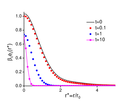
Figure 1: (color online) Ideal gas Pauli pair potential as a function of $r^{*}=r/r_{0}$ for $t=0,0.1,1,10$.

Generally, the potential is positive, finite at $r=0$ (Pauli exclusion), and monotonically decreasing. The behavior is exponential at small $r$, but an $r^{-2\text{ }}$algebraic tail develops for small $t$. This arises from the direct correlation function $c^{(2)}(r)$ in (63). Classical statistical mechanics does not exist for such a long range potential and it would appear that the equivalent classical system proposed here fails even for this simplest case of an ideal Fermi gas. However, this problem is ”cured” for the corresponding case of classical Coulomb interactions with the same long range problem by adding a uniform neutralizing background (the one component plasma). The same procedure can be used here, i.e., a classical system is considered where the pair potential is supplemented in the Hamiltonian by a corresponding uniform compensating background. The pressure equation (27) is modified due to this background by the replacement of $g_{c}(\mathbf{r,r}^{\prime})$ by $g_{c}(\mathbf{r,r}^{\prime})-1$, and (61) becomes

$$\frac{\beta_{c}}{\beta}=\frac{n}{\beta p}\left[1-\frac{1}{6}n\int d\mathbf{r}h(r)\mathbf{r}\cdot\nabla\beta_{c}\phi_{c}(r)\right].$$ (65)

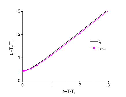
Figure 2: (color online) Ideal gas reduced classical temperature $t_{c}=T_{c}/T_{F}$ as a function of $t=T/T_{F}$ . Also shown is the result of PDW.

Figure 2 shows the classical temperature relative to the Fermi temperature, $\beta_{F}/\beta_{c}\equiv t_{c}$, as a function of $t$ obtained from (65). It is seen that the classical temperature $T_{c}$ remains finite at $T=0$ in all cases, and crosses over to $T_{c}=T$ at high temperatures. The PDW model postulates the form $T_{c}=\left(T^{2}+T_{0}^{2}\right)^{1/2}$. The model originally uses the average energy per particle at $T=0$ to evaluate $T_{0}=2T_{F}/5$. The result from (65) is quite close $T_{c}\left(t=0\right)\sim 0.43T_{F}.$ To compare the dependence at finite $t$, the PDW form is also shown in Figure 2 with $T_{0}=T_{c}\left(t=0\right)$. It is seen that the results are quite similar although the PDW form has a somewhat faster cross over to the classical limit.

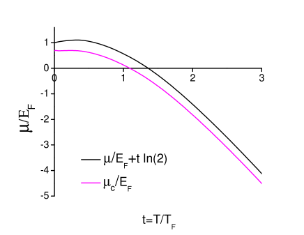
Figure 3: (color online) Ideal gas dimensionless chemical potential $\mu_{c}/E_{F}$ as a function of $t$. Also shown is the corresponding quantum chemical potential $\mu/E_{F}+t\ln 2$.

Figure 3 shows similar results for $\mu_{c}/E_{F}$ as a function of $t$ obtained from (62). Also shown is the result for the quantum $\mu/E_{F}$. Both forms depend only on $t$ (independent of $r_{s}$). At high temperatures the chemical potential of the representative system goes over to $\ln(n\lambda^{3})$ as in equation (62) while the quantum chemical potential goes over to $\ln(n\lambda^{3}/2)$. They differ by a factor of $\ln(2)$ at high temperatures due to the internal spin degrees of freedom in the quantum calculation. This is accommodated in the comparison shown in Figure 3.

With the parameters of the equivalent classical system determined, it is now possible to calculate any desired property of the ideal quantum gas by classical methods. Since the pressure is given exactly by the definition of the classical - quantum correspondence equations, it is useful to consider the internal energy. First, note that all the dimensionless thermodynamic quantities of both the quantum and classical ideal gas depend on only one thermodynamic parameter $z=e^{\beta\mu}$. In particular

$$\beta_{c}p_{c}\lambda_{c}^{3}=G(z).$$ (66)

The specific form for $G(z)$ is not required for the present discussion. The corresponding quantum result is $\beta p\lambda^{3}=f_{3/2}(z)$, where $f_{3/2}(z)$ is the Fermi integral of Appendix B, (105). Although $G(z)$ and $f_{3/2}(z)$ are quite different, the fact that they both depend only on $z$ implies that the relationship among different thermodynamic properties is the same in both classical and quantum cases. For example, the energy per particle is determined from the pressure via the thermodynamic definition (50) with (62)

$$\widetilde{E}_{c}=-VG(z)\frac{\partial\lambda_{c}^{-3}}{\partial\beta_{c}}\mid_{z_{c}}=\frac{2}{3}p_{c}V$$ (67)

The contribution from $\partial G(z)/\partial\beta_{c}\mid_{z_{c},V}$ vanishes since $z=z(z_{c})$. This follows on dimensional grounds since $z$ is dimensionless, and there is no additional energy scale to make $\beta_{c}$ dimensionless. Hence the classical calculation gives the known exact quantum result. This non-trivial result for a classical interacting system is a strong confirmation of the effective classical map defined here. As noted in the last section, it can be verified that the classical average of the classical Hamiltonian does not give the correct relationship to the pressure. Instead it is necessary to define the internal energy thermodynamically, as is done in (67). In a similar way it is verified that the relationship of the classical entropy to the pressure and density is the same as in the quantum case

$$T_{c}S_{c}=\frac{5}{2}p_{c}V-\mu_{c}\overline{N}_{c}.$$ (68)

This is a form of the Sackur-Tetrode equation valid for the quantum case. It is emphasized that these simple ideal quantum gas results are being retained for the more complex effective classical system with pair interactions via the Pauli potential.

V Weak Coupling Pair Potential

For systems with real interactions $\phi(\mathbf{q}_{1},\mathbf{q}_{2})$ between  the particles, the classical pair potential will have the form

$$\beta_{c}\phi_{c}(\mathbf{q}_{1},\mathbf{q}_{2})=\left(\phi_{c}(\mathbf{q}_{1},\mathbf{q}_{2})\right)^{(0)}+\Delta(\mathbf{q}_{1},\mathbf{q}_{2}),$$ (69)

where $\left(\phi_{c}(\mathbf{q}_{1},\mathbf{q}_{2})\right)^{(0)}$ is the ideal gas Pauli potential and $\Delta(\mathbf{q}_{1},\mathbf{q}_{2})$ denotes the contribution to the effective potential from the real pair potential. Obviously, in the classical limit $\Delta(\mathbf{q}_{1},\mathbf{q}_{2})\rightarrow\beta\phi(\mathbf{q}_{1},\mathbf{q}_{2})$. Another exact limit is the weak coupling limit for which the direct correlation function becomes proportional to the potential Hansen , or stated inversely,

$$\beta_{c}\phi_{c}(r)\rightarrow-c(r),\hskip 14.45377pt\left(\beta_{c}\phi_{c}(r)\right)^{(0)}\rightarrow-c^{(0)}(r).$$ (70)

Thus a possible approximation incorporating this limit is

$$\beta_{c}\phi_{c}(r)\rightarrow\left(\beta_{c}\phi_{c}(r)\right)^{(0)}-\left(c(r)-c^{(0)}(r)\right)^{(w)},$$ (71)

where $\left(c(r)-c^{(0)}(r)\right)^{(w)}$ denotes a weak coupling calculation of the direct correlation functions from the Ornstein - Zernicke equation (30)

$$-\left(\beta_{c}\phi_{c}(r)\right)^{(w)}=h^{(w)}\left(r\right)+n\int d\mathbf{r}^{\prime}\left(\beta_{c}\phi_{c}(\left|\mathbf{r-r}^{\prime}\right|)\right)^{(w)}h^{(w)}(r^{\prime}),$$ (72)

with $h^{w}\left(r\right)$ being the quantum hole function in its weak coupling form. In the following companion paper this approximation is applied to the electron gas (jellium) for which the weak coupling form is given by the random phase approximation.

To further interpret approximation (71) consider a uniform system and rewrite $\Delta(\mathbf{q}_{1},\mathbf{q}_{2})=\Delta(\left|\mathbf{q}_{1}-\mathbf{q}_{2}\right|)$ in terms of the static structure factor

$$S\left(k\right)=1+n\int d\mathbf{r}e^{i\mathbf{k\cdot r}}h(r),$$ (73)

$$\Delta(\left|\mathbf{q}_{1}-\mathbf{q}_{2}\right|) =\frac{1}{n}\int\frac{d\mathbf{k}}{\left(2\pi\right)^{3}}e^{-i\mathbf{k\cdot}\left(\mathbf{q}_{1}-\mathbf{q}_{2}\right)}\left(\frac{1}{S(k)}-\frac{1}{S^{(0)}(k)}\right)^{(w)}$$

$$=\beta\phi(\left|\mathbf{q}_{1}-\mathbf{q}_{2}\right|)-\int d\mathbf{q}G(\mathbf{q})\beta\phi(\left|\mathbf{q}_{1}-\mathbf{q}_{2}-\mathbf{q}\right|)$$ (74)

Here $G(\mathbf{q})$ is known as the local field corrections in linear response for the classical system. It is seen that the quantum corrections to $\beta\phi(\left|\mathbf{q}_{1}-\mathbf{q}_{2}\right|)$ can be interpreted as local field corrections STLS , Tanaka86 , although due to quantum effects rather than classical correlations. In the case of jellium, the qualitative features of (74) are a regularization of the Coulomb singularity at $\mathbf{q}_{1}=\mathbf{q}_{2}$, and cross-over to an asymptotic Coulomb decay for large $\left|\mathbf{q}_{1}-\mathbf{q}_{2}\right|$ with effective coupling constant given by the exact perfect screening sum rule.

VI Discussion

The objective here has been to define an effective classical equilibrium statistical mechanics that corresponds to a chosen quantum system of interest. The motivation is to allow application of existing strong coupling classical methods (e.g. liquid state theory, MD simulation) to calculate properties of the quantum system under conditions for which current theoretical approaches are not adequate. The correspondence has been defined by equivalence of the pressures, densities, and pair correlation functions for the classical and quantum systems. In this way, the relevant parameters for the classical grand ensemble are fixed - the temperature, local chemical potential, and pair potential. These classical parameters were given a more explicit representation in terms of the quantum parameters by inverting the classical many-body problem using the HNC integral equations. Formal questions such as the existence of this inversion have not been addressed, and only presumed to hold. A counter example is given by the classical representation of jellium, where the equivalence of pressures is not possible under conditions of negative pressures.

The three correspondence conditions of section II are not unique, and other choices may be preferred in specific applications. Furthermore, applications require the introduction of appropriate approximate forms for these correspondence conditions that should be tailored to the particular system at hand. The special case of a uniform ideal Fermi gas was illustrated using the HNC integral equation to determine the parameters of the effective classical system. A peculiarity is the long range nature of the effective pair potential at very low temperatures, requiring the introduction of a compensating uniform background. The resulting classical thermodynamics was shown to reproduce the exact relationships of various thermodynamic functionals (e.g., pressure, internal energy, entropy).

The non-uniform ideal Fermi gas is more interesting and its representation as a functional of the local density is a fundamental problem within density functional theory DFT . Approximations such as the Thomas-Fermi representation have limited applicability. An effective classical representation along the lines described here would provide access to better approximations, since the functional dependence on density for the classical system is simple.

A weak coupling approximation for the effective pair potential in systems with real forces was described in the last section. With that pair potential known, the effective chemical potential and effective temperature can be calculated. This is illustrated in the following companion paper for the uniform electron gas Dutta12 . The pair correlation function is calculated for a wide range of densities and temperatures, and good agreement is obtained with diffusion Monte Carlo results at zero temperature and recently reported Restricted Path Integral Monte Carlo results at finite temperatures.

A second application in that paper is to shell structure for charges confined in a harmonic trap. Classically, shell structure arises only from Coulomb correlations Wrighton09 . A preliminary investigation there shows new origins of shell structure due to diffraction and exchange, even in the absence of Coulomb correlations (mean field approximation).

VII Acknowledgements

This research has been supported by NSF/DOE Partnership in Basic Plasma Science and Engineering award DE-FG02-07ER54946 and by US DOE Grant DE-SC0002139.

Appendix A Exact Coupled Equations for $n_{c}(\mathbf{r})$ and $g_{c}\left(\mathbf{r,r}^{\prime}\right)$.

The objective of this appendix is to outline the origin of the exact equations (28) - (30) for the classical density and pair correlation function. First, make a change of thermodynamic variables from temperature and chemical potential $\beta_{c},\mu_{c}(\mathbf{r})$ to temperature and density $\beta_{c},n_{c}(\mathbf{r})$ by the Legendre transformation

$$F_{c}(\beta_{c}\mid n_{c})=\Omega_{c}\left(\beta_{c}\mid\mu_{c}\right)+\int d\mathbf{r}\mu_{c}\left(\mathbf{r}\right)n_{c}\left(\mathbf{r}\right),$$ (75)

where now the free energy is a functional of the classical density rather than $\mu_{c}\left(\mathbf{r}\right)$. Their relationship is given by the first derivative

$$\frac{\delta F_{c}}{\delta n_{c}(\mathbf{r})}=\mu_{c}(\mathbf{r}).$$ (76)

Here, and throughout this Appendix derivatives are taken at constant $\phi_{c}$, so the densities involved are those defined as in (18). The free energy is now divided into its ideal gas contribution $F_{c}^{(0)}=-\beta_{c}^{-1}\int d\mathbf{r}\left[1-\ln\left(n_{c}\left(\mathbf{r}\right)\lambda_{c}^{3}\right)\right]n_{c}\left(\mathbf{r}\right)$, where $\lambda_{c}=\left(2\pi\hbar^{2}\beta_{c}/m\right)^{1/2}$, and the remainder $F_{c,ex}$ (excess free energy), so that (76) becomes an equation for the density

$$\ln\left(n_{c}\left(\mathbf{r};\beta_{c}\right)\lambda_{c}^{3}\right)=\beta_{c}\mu_{c}(\mathbf{r})+c_{c}^{(1)}\left(\mathbf{r};\beta_{c}\mid n_{c}\right).$$ (77)

Here $c_{c}^{(1)}\left(\mathbf{r}\mid n_{c}\right)$ is the first of a family of functions (direct correlation functions) defined by derivatives of the free energy

$$c_{c}^{(m)}\left(\mathbf{r}_{1},..,\mathbf{r}_{m};\beta_{c}\mid n_{c}\right)\equiv-\beta\frac{\delta^{m}F_{c,ex}}{\delta n_{c}(\mathbf{r}_{1})..\delta n_{c}(\mathbf{r}_{m})}$$ (78)

Equation (77) relates the density $n_{c}(\mathbf{r})$ to a given external potential (recall $\mu_{c}(\mathbf{r})=\mu_{c}-\phi_{c,ext,}(\mathbf{r})$). Consider now a different external potential given by $\phi_{c,ext,}(\mathbf{r})+\phi_{c}(\mathbf{r,r}^{\prime})$ and associated density $n_{c}(\mathbf{r,r}^{\prime})$. This external potential corresponds to the original one $\phi_{c,ext,}(\mathbf{r})$ plus a new source of potential of the same form as would occur if another particle were added at the point $\mathbf{r}^{\prime}$. It follows that this new density is proportional to the pair correlation function for the original system Hansen

$$n_{c}\left(\mathbf{r,r}^{\prime}\right)=n_{c}\left(\mathbf{r}\right)g_{c}\left(\mathbf{r,r}^{\prime}\right).$$ (79)

The equation corresponding to (77) for this new external potential is

$$\ln\left(n_{c}\left(\mathbf{r}\right)g_{c}\left(\mathbf{r,r}^{\prime}\right)\lambda_{c}^{3}\right)=\beta_{c}\mu_{c}(\mathbf{r})-\beta_{c}\phi_{c}(\mathbf{r,r}^{\prime})+c_{c}^{(1)}\left(\mathbf{r};\beta_{c}\mid n_{c}g_{c}\right).$$ (80)

Finally, subtracting (77) from (80) gives the desired equation for $g_{c}\left(\mathbf{r,r}^{\prime}\right)$

$$\ln\left(g_{c}\left(\mathbf{r,r}^{\prime}\right)\lambda_{c}^{3}\right)=-\beta_{c}\phi_{c}(\mathbf{r,r}^{\prime})+c_{c}^{(1)}\left(\mathbf{r};\beta_{c}\mid n_{c}g_{c}\right)-c_{c}^{(1)}\left(\mathbf{r};\beta_{c}\mid n_{c}\right).$$ (81)

The notation used implies that the functional $c_{c}^{(1)}\left(\mathbf{r};\beta_{c}\mid\cdot\right)$ in both (77) and (80) are the same. This follows from density functional theory where it is demonstrated that the free energy is a universal functional of the density, the same for all external potentials. Equations (28) and (29) now follow directly from (77) and (81) and the identity

$$c_{c}^{(1)}\left(\mathbf{r};\beta_{c}\mid X\right) =c_{c}^{(1)}\left(\mathbf{r};\beta_{c}\mid Y\right)+\int_{0}^{1}d\alpha\partial_{\alpha}c_{c}^{(1)}\left(\mathbf{r};\beta_{c}\mid\alpha X+\left(1-\alpha\right)Y\right)$$

$$=c_{c}^{(1)}\left(\mathbf{r};\beta_{c}\mid Y\right)+\int_{0}^{1}d\alpha\int d\mathbf{r}^{\prime}\frac{\delta c_{c}^{(1)}\left(\mathbf{r};\beta_{c}\mid\alpha X+\left(1-\alpha\right)Y\right)}{\delta n_{c}\left(\mathbf{r}^{\prime}\right)}\left(X\left(\mathbf{r}^{\prime}\right)-Y\left(\mathbf{r}^{\prime}\right)\right)$$

$$=c_{c}^{(1)}\left(\mathbf{r};\beta_{c}\mid Y\right)+\int_{0}^{1}d\alpha\int d\mathbf{r}^{\prime}c_{c}^{(2)}\left(\mathbf{r,r}^{\prime};\beta_{c}\mid\alpha X+\left(1-\alpha\right)Y\right)\left(X\left(\mathbf{r}^{\prime}\right)-Y\left(\mathbf{r}^{\prime}\right)\right)$$ (82)

with appropriate choices for $X$ and $Y$.

The Ornstein - Zernicke equation (30) is an identity obtained as follows. The second functional derivative of the grand potential is related to the pair correlation function by

$$\frac{\delta^{2}\left(-\beta_{c}\Omega_{c}\right)}{\delta\mu_{c}\left(\mathbf{r}\right)\mu_{c}\left(\mathbf{r}^{\prime}\right)}=\frac{\delta n_{c}\left(\mathbf{r}^{\prime}\right)}{\delta\mu_{c}\left(\mathbf{r}\right)}=\beta_{c}n_{c}\left(\mathbf{r}^{\prime}\right)\left[\delta\left(\mathbf{r-r}^{\prime}\right)+n_{c}\left(\mathbf{r}\right)\left(g_{c}\left(\mathbf{r,r}^{\prime}\right)-1\right)\right],$$ (83)

Similarly, the second derivative of the free energy is

$$\frac{\delta^{2}F_{c}}{\delta n_{c}\left(\mathbf{r}^{\prime}\right)\delta n_{c}\left(\mathbf{r}\right)}=\frac{\delta\mu_{c}(\mathbf{r})}{\delta n_{c}\left(\mathbf{r}^{\prime}\right)}=\beta_{c}^{-1}n_{c}\left(\mathbf{r}\right)^{-1}\left[\delta\left(\mathbf{r-r}^{\prime}\right)-n_{c}\left(\mathbf{r}\right)c_{c}^{(2)}\left(\mathbf{r,r}^{\prime}\mid n_{c}\right)\right].$$ (84)

Then the chain rule

$$\int d\mathbf{r}^{\prime\prime}\frac{\delta n_{c}\left(\mathbf{r}\right)}{\delta\mu_{c}\left(\mathbf{r}^{\prime\prime}\right)}\frac{\delta\mu_{c}(\mathbf{r}^{\prime\prime})}{\delta n_{c}\left(\mathbf{r}^{\prime}\right)}=\delta\left(\mathbf{r-r}^{\prime}\right)$$ (85)

can be written

$$\int d\mathbf{r}^{\prime\prime}\left[\delta\left(\mathbf{r-r}^{\prime\prime}\right)+n_{c}\left(\mathbf{r}\right)\left(g_{c}\left(\mathbf{r,r}^{\prime\prime}\right)-1\right)\right]\left[\delta\left(\mathbf{r}^{\prime\prime}\mathbf{-r}^{\prime}\right)-n_{c}\left(\mathbf{r}^{\prime\prime}\right)c_{c}^{(2)}\left(\mathbf{r}^{\prime\prime}\mathbf{,r}^{\prime}\mid n_{c}\right)\right]=\delta\left(\mathbf{r-r}^{\prime}\right).$$ (86)

This gives the Ornstein-Zernicke equation (30).

Appendix B Inhomogeneous Ideal Fermi Gas

The thermodynamic and structural properties of an inhomogeneous ideal Fermi gas are straightforward to calculate in a representation that diagonalizes the effective single particle Hamiltonian

$$\left(\frac{\widehat{p}^{2}}{2m}-\mu(\widehat{\mathbf{r}})\right)\psi_{\mathbf{k}}\left(\mathbf{r}\right)=\epsilon_{\mathbf{k}}\psi_{\mathbf{k}}\left(\mathbf{r}\right),$$ (87)

where $\mathbf{k}$ labels the corresponding quantum numbers. For Fermions with spin $s$, the quantum numbers are labeled by $\kappa=\left(s,\mathbf{k}\right)$. The Hamiltonian in second quantized form is then simply

$$H=\sum_{\kappa}\epsilon_{\mathbf{k}}a_{\kappa}^{\dagger}a_{\kappa},$$ (88)

where $a_{\kappa}^{\dagger},a_{\kappa}$ are the creation and annihilation operators for occupation of the states $\left\{\psi_{\mathbf{k}}\right\}$. Then the pressure is found directly from evaluation of the grand potential $\Omega_{c}$

$$p(\beta \mid\mu)V=\beta^{-1}\sum_{\kappa}\ln\left(1+e^{-\beta\epsilon_{\mathbf{k}}}\right)=\beta^{-1}Tr^{(1)}\ln\left(1+e^{-\beta\left(\frac{\widehat{p}^{2}}{2m}-\mu(\widehat{\mathbf{r}})\right)}\right)$$

$$=\left(2s+1\right)\beta^{-1}\int d\mathbf{r}\left\langle\mathbf{r}\right|\ln\left(1+e^{-\beta\left(\frac{\widehat{p}^{2}}{2m}-\mu(\widehat{\mathbf{r}})\right)}\right)\left|\mathbf{r}\right\rangle,$$ (89)

where a coordinate representation has been used in the last expression.

The local density and pair correlation function are obtained from the one an two particle density matricies. In the diagonal representation these are

$$\rho^{(1)}\left(\kappa_{1};\kappa_{2}\right)=\left\langle a_{\kappa_{1}}^{\dagger}a_{\kappa_{2}}\right\rangle=\left\langle a_{\kappa_{1}}^{\dagger}a_{\kappa_{1}}\right\rangle\delta_{\kappa_{1},\kappa_{2}}$$ (90)

$$\rho^{(2)}\left(\kappa_{1},\kappa_{2};\kappa_{3},\kappa_{4}\right)=\left\langle a_{\kappa_{1}}^{\dagger}a_{\kappa_{2}}^{\dagger}a_{\kappa_{4}}a_{\kappa_{3}}\right\rangle=\left(\delta_{\kappa_{1},\kappa_{3}}\delta_{\kappa_{2},\kappa_{4}}-\delta_{\kappa_{1},\kappa_{4}}\delta_{\kappa_{2},\kappa_{3}}\right)\left\langle a_{\kappa_{1}}^{\dagger}a_{\kappa_{1}}\right\rangle\left\langle a_{\kappa_{2}}^{\dagger}a_{\kappa_{2}}\right\rangle$$ (91)

Where the mean occupation number is

$$\left\langle a_{\kappa}^{\dagger}a_{\kappa^{\prime}}\right\rangle=\delta_{\kappa,\kappa^{\prime}}\left(e^{\beta\epsilon_{\mathbf{k}}}+1\right)^{-1}.$$ (92)

The coordinate representations are

$$\rho^{(1)}\left(\mathbf{r,}\sigma_{1};\mathbf{r}^{\prime},\sigma_{2}\right) =\sum_{\mathbf{k}_{1},\mathbf{k}_{2}}\psi_{\kappa_{1}}^{\ast}\left(\mathbf{r}\right)\psi_{\kappa_{2}}\left(\mathbf{r}^{\prime}\right)\left\langle a_{\kappa_{1}}^{\dagger}a_{\kappa_{2}}\right\rangle=\delta_{\sigma_{1},\sigma_{2}}\left\langle\mathbf{r}\right|\ln\left(e^{\beta\left(\frac{\widehat{p}^{2}}{2m}-\mu(\widehat{\mathbf{r}})\right)}+1\right)^{-1}\left|\mathbf{r}^{\prime}\right\rangle$$

$$\equiv\delta_{\sigma_{1},\sigma_{2}}n\left(\mathbf{r},\mathbf{r}^{\prime}\right)$$ (93)

$$\rho^{(2)}\left(\mathbf{r}_{1},\sigma_{1},\mathbf{r}_{2},\sigma_{2};\mathbf{r}_{1}^{\prime},\sigma_{3},\mathbf{r}_{2}^{\prime},\sigma_{4}\right) =\sum_{\mathbf{k}_{1}..\mathbf{k}_{6}}\psi_{\kappa_{1}}^{\ast}\left(\mathbf{r}_{1}\right)\psi_{\kappa_{2}}^{\ast}\left(\mathbf{r}_{2}\right)\psi_{\kappa_{3}}\left(\mathbf{r}_{1}^{\prime}\right)\psi_{\kappa_{4}}\left(\mathbf{r}_{2}^{\prime}\right)\left\langle a_{\kappa_{1}}^{\dagger}a_{\kappa_{2}}^{\dagger}a_{\kappa_{4}}a_{\kappa_{3}}\right\rangle$$

$$=\delta_{\sigma_{1},\sigma_{3}}\delta_{\sigma_{2},\sigma_{4}}\sum_{\mathbf{k}_{1}}\psi_{\kappa_{1}}^{\ast}\left(\mathbf{r}_{1}\right)\psi_{\kappa_{1}}\left(\mathbf{r}_{1}^{\prime}\right)\left\langle a_{\kappa_{1}}^{\dagger}a_{\kappa_{1}}\right\rangle\sum_{\mathbf{k}_{2}}\psi_{\kappa_{2}}^{\ast}\left(\mathbf{r}_{2}\right)\psi_{\kappa_{2}}\left(\mathbf{r}_{2}^{\prime}\right)\left\langle a_{\kappa_{2}}^{\dagger}a_{\kappa_{2}}\right\rangle$$

$$-\delta_{\sigma_{1},\sigma_{4}}\delta_{\sigma_{2},\sigma_{3}}\sum_{\mathbf{k}_{1}}\psi_{\kappa_{1}}^{\ast}\left(\mathbf{r}_{1}\right)\psi_{\kappa_{1}}\left(\mathbf{r}_{2}^{\prime}\right)\left\langle a_{\kappa_{1}}^{\dagger}a_{\kappa_{1}}\right\rangle\sum_{\mathbf{k}2}\psi_{\kappa_{2}}^{\ast}\left(\mathbf{r}_{2}\right)\psi_{\kappa_{2}}\left(\mathbf{r}_{1}^{\prime}\right)\left\langle a_{\kappa_{2}}^{\dagger}a_{\kappa_{2}}\right\rangle$$ (94)

The diagonal elements are

$$\rho^{(1)}\left(\mathbf{r,}\sigma_{1};\mathbf{r},\sigma_{1}\right)=n\left(\mathbf{r},\mathbf{r}\right)$$ (95)

$$\rho^{(2)}\left(\mathbf{r}_{1},\sigma_{1},\mathbf{r}_{2},\sigma_{2};\mathbf{r}_{1},\sigma_{1},\mathbf{r}_{2},\sigma_{2}\right) =\rho^{(1)}\left(\mathbf{r}_{1}\mathbf{,}\sigma_{1};\mathbf{r}_{1},\sigma_{1}\right)\rho^{(1)}\left(\mathbf{r}_{2}\mathbf{,}\sigma_{2};\mathbf{r}_{2},\sigma_{2}\right)$$

$$-\delta_{\sigma_{1},\sigma_{2}}\rho^{(1)}\left(\mathbf{r}_{1}\mathbf{,}\sigma_{1};\mathbf{r}_{2},\sigma_{1}\right)\rho^{(1)}\left(\mathbf{r}_{2}\mathbf{,}\sigma_{2};\mathbf{r}_{1},\sigma_{2}\right)$$ (96)

Finally, the density and pair correlation function are identified from the summation over spin states

$$n(\mathbf{r})=\sum_{\sigma_{1}}\rho^{(1)}\left(\mathbf{r,}\sigma_{1};\mathbf{r},\sigma_{1}\right)=\left(2s+1\right)n\left(\mathbf{r},\mathbf{r}\right)$$ (97)

$$n(\mathbf{r}_{1})n(\mathbf{r}_{2})g\left(\mathbf{r}_{1},\mathbf{r}_{2}\right)=\sum_{\sigma_{1},\sigma_{2}}\rho^{(2)}\left(\mathbf{r}_{1},\sigma_{1},\mathbf{r}_{2},\sigma_{2};\mathbf{r}_{1},\sigma_{1},\mathbf{r}_{2},\sigma_{2}\right)=n(\mathbf{r}_{1})n(\mathbf{r}_{2})-\left(2s+1\right)n\left(\mathbf{r}_{1},\mathbf{r}_{2}\right)n\left(\mathbf{r}_{2},\mathbf{r}_{1}\right)$$ (98)

This gives the results (56) and (57).

The local density and pair correlation function are determined from the function $n\left(\mathbf{r},\mathbf{r}^{\prime}\right)$ obtained from the single particle density matrix (93),

$$n(\mathbf{r,r}^{\prime})=\left\langle\mathbf{r}\right|\left(e^{\beta\left(\frac{\widehat{p}^{2}}{2m}-\mu(\widehat{\mathbf{r}})\right)}+1\right)^{-1}\left|\mathbf{r}^{\prime}\right\rangle.$$ (99)

In the local density approximation of the text, $\mu(\widehat{\mathbf{r}})\rightarrow\mu(\mathbf{R})$, where $\mathbf{R=}\left(\mathbf{r+r}^{\prime}\right)/2$, this becomes (60)

$$n(\mathbf{r,r}^{\prime})=\frac{1}{h^{3}}\int d\mathbf{p}e^{\frac{i}{\hbar}\mathbf{p\cdot}\left(\mathbf{r-r}^{\prime}\right)}\left(e^{\beta(\frac{p^{2}}{2m}-\mu(\mathbf{R}))}+1\right)^{-1}.$$ (100)

Further simplification is possible to get

$$n(\mathbf{r,r}^{\prime})\lambda^{3}=\frac{2\lambda}{\pi\left|\mathbf{r-r}^{\prime}\right|}\int_{0}^{\infty}dxx\left(z^{-1}(\mathbf{R})e^{x^{2}}+1\right)^{-1}\sin\left(2\sqrt{\pi}x\left|\mathbf{r-r}^{\prime}\right|\mathbf{/}\lambda\right),$$ (101)

with

$$z(\mathbf{R})=e^{\beta\mu(\mathbf{R})}$$ (102)

Accordingly the density and pressure simplify to

$$n(\mathbf{r})\lambda^{3}=\left(2s+1\right)n(\mathbf{r,r})\lambda^{3}=\left(2s+1\right)f_{3/2}(z(\mathbf{r})),$$ (103)

$$\beta p\lambda^{3}=\frac{1}{V}\int d\mathbf{r}\left(2s+1\right)f_{5/2}(z(\mathbf{r})),$$ (104)

with  the definitions

$$f_{3/2}(z)=\frac{4}{\sqrt{\pi}}\int_{0}^{\infty}dxx^{2}\left(z^{-1}e^{x^{2}}+1\right)^{-1},\hskip 14.45377ptf_{5/2}(z)=\frac{8}{3\sqrt{\pi}}\int_{0}^{\infty}dxx^{4}\left(z^{-1}e^{x^{2}}+1\right)^{-1}.$$ (105)

References

• [1] J-P Hansen and I. MacDonald, Theory of Simple Liquids, (Academic Press, San Diego, CA, 1990).
• [2] J. Lutsko, Recent Developments in Classical Density Functional Theory, Adv. Chem. Phys. 144, S. Rice, ed. (J. Wiley, Hoboken, NJ, 2010).
• [3] R. Rozner, D. Hammer, and T. Rothman Basic Research Needs in High Energy Density Laboratory Physics, (U.S. Dept. of Energy, 2010), Chapter 6 and references therein; R.P. Drake,”High Energy Density Physics”, Phys. Today 63, 28-33 (2010) and refs. therein.
• [4] G.E. Uhlenbeck, L. Gropper, Phys. Rev. 41 (1932) 79.
• [5] T. Morita, Prog. Theor. Phys. 20, 920 (1958); 23, 829 (1960).
• [6] G. Kelbg, Ann. Phys. 12, 219 (1963).
• [7] F. Lado, J. Chem. Phys. 47, 5369 (1967).
• [8] T. Dunn and A. Broyles, Phys. Rev. 157, 1 (1967).
• [9] For additional early references see W. Ebeling, A. Filinov, M. Bonitz, V. Filinov, and T. Pohl, J. Phys. A 39, 4309 (2006); A. Filinov, V. Golubnychiy, M. Bonitz, W. Ebeling, and J. Dufty, Phys. Rev. E 70, 046411 (2004).
• [10] J. Dufty, S. Dutta, M. Bonitz, and A. Filinov, Int. J. Quant. Chem. 109, 3082 (2009)
• [11] C. Jones and M. Murillo, High Energy Density Physics 3, 379 (2007); F. Graziani et al, High Energy Density Physics 8,105 (2012).
• [12] M. W. C. Dharma-wardana and F. Perrot, Phys. Rev. Lett. 84, 959 (2000); F. Perrot and M. W. C. Dharma-wardana, Phys. Rev. B 62, 16536 (2000).
• [13] C. Deutsch, Phys. Lett. A 60, 317 (1977); H. Minoo, M. Gombert, and C. Deutsch, Phys. Rev. A 23, 924 (1981).
• [14] M. W. C. Dharma-wardana, Int. J. Quant. Chem. 112, 53 (2012).
• [15] J. W. Dufty and S. Dutta, Contrib. Plasma Phys. 52, 100 (2012).
• [16] S. Dutta and J. Dufty, Classical Representation of a Quantum System at Equilibrium: Applicatations, following paper in this journal.
• [17] S. Tanaka and S. Ichimaru, J. Phys. Soc. Japan 55, 2278 (1986); K. S. Singwi, M. P. Tosi, R. H. Land, and A. Sj lander, Phys. Rev. 176, 589 (1968); P. Vashista and K. S. Singwi, Phys. Rev. B 6, 875 (1972).
• [18] P. Attard, J. Chem. Phys. 91, 3072 (1989), equation (18).
• [19] J. Wrighton, J. W. Dufty, H. Kählert, and M. Bonitz, Phys. Rev. E 80, 066405 (2009).
• [20] J. Wrighton, H. Kählert, T. Ott, P. Ludwig, H. Thomsen, J. Dufty, and M. Bonitz, Contrib. Plasma Phys. 52, 45 (2012).
• [21] Density Functional Theory: An Advanced Course, E. Engel and R.M. Dreizler (Springer, Heidelberg, 2011).
• [22] M. Baus and J.P. Hansen, Phys. Rep. 59 (1980) 1.
• [23] Singwi K. S., Tosi M. P., Land R. H. and Sjölander A., Phys. Rev., 179 (1968)
• [24] J. W. Dufty and S. Trickey, Phys. Rev. B 84, 125118 (2011).