IPMU 12-0209

Neutron Electric Dipole Moment
Induced by the Strangeness Revisited

Kaori Fuyuto^a, Junji Hisano^a,b, Natsumi Nagata^a,c

^aDepartment of Physics, Nagoya University, Nagoya 464-8602, Japan
^bKavli IPMU, University of Tokyo, Kashiwa 277-8584, Japan
^cDepartment of Physics, University of Tokyo, Tokyo 113-0033, Japan

We have revisited the calculation of the neutron electric dipole moment in the presence of the CP-violating operators up to dimension five based on the chiral perturbation theory. Especially, we focus on the contribution of strangeness content. In the calculation, we extract the nucleon matrix elements of scalar-type quark operators from the results of the lattice QCD simulations, while those of the dipole-type quark-gluon operators are evaluated by using the method of the QCD sum rules. As a result, it is found that although the strangeness quantity in nucleon is small, the contribution of the chromoelectric dipole moment of strange quark may be still sizable, and thus may offer a sensitive probe for the CP-violating interactions in physics beyond the Standard Model.

1 Introduction

The neutron electric dipole moment (EDM) is one of the physical quantities that are extremely sensitive to the CP violation in the high-energy theories beyond the Standard Model (SM). The contribution of the SM electroweak interactions to the neutron EDM, $d_{n}$, has been evaluated as $d_{n}\sim 10^{-(31-32)}~{}e\cdot{\rm cm}$ [1, 2], which is still below the experimental limit $|d_{n}|<2.9\times 10^{-26}~{}e\cdot{\rm cm}$ [3] by several orders of magnitude. Therefore, the neutron EDM provides a clean, background-free probe of the CP-violating interactions in physics beyond the SM, as well as the so-called $\theta$ term in the QCD Lagrangian. In order to look for the neutron EDM, various experiments have been proposed and put into practice. Their sensitivities are expected to be much improved mainly due to the use of ultra cold neutrons. For instance, the nEDM collaboration at the Paul-Scherrer Institute (PSI) [4] aims at giving a sensitivity of $\sim 5\times 10^{-27}~{}e~{}{\rm cm}$, and finally getting into the regime of $10^{-28}~{}e~{}{\rm cm}$.

From a theoretical point of view, on the other hand, one needs to interpret the value of or the limits on the neutron EDM provided by experiments in terms of the CP violation at parton level. To that end, there have been a lot of previous efforts to derive precise relations between the CP-violating interactions and the neutron EDM. At the moment, only an approach exploiting the QCD sum rules [5, 6] provides a systematic treatment for the derivation, which has been conducted in various literature [7, 8, 9, 10, 11, 12, 13, 14]. In this approach, it is possible to include the contribution of the QCD $\theta$ term, the quark EDMs, and the quark chromoelectric dipole moments (CEDMs) on an equal footing. The QCD lattice simulations also offer a promising way of evaluating the neutron EDM induced by such CP-violating interactions. Although their results are not precise enough at present [15, 16, 17, 18, 19], we expect that the lattice simulations eventually will be able to determine it with high accuracy.

An alternative, in fact a traditional, approach to the calculation of the neutron EDM is based on the chiral perturbation theory. This method has the advantage of being able to include sea quark effects indirectly, while in the QCD sum rule method such effects appear only at the higher orders. The contribution of the QCD $\theta$ term to the neutron EDM has been evaluated in Refs. [20, 21, 22, 23, 24]. In Ref. [25, 26, 27], the quark CEDM contributions are also discussed. While the Peccei-Quinn (PQ) symmetry [28] is often considered in order to suppress the $\theta$ term and solve the strong CP problem, it is important to evaluate the neutron EDM induced by the higher dimensional operators, such as the quark CEDMs, which are sensitive to TeV-scale physics. In the calculation, the effects of the CP-violating operators are incorporated into the CP-odd meson-baryon couplings, which are obtained by evaluating the nucleon matrix elements of the CP-even quark scalar operators. The authors in Ref. [25] extracted the matrix elements from the baryon mass splittings and the nucleon sigma terms also evaluated in terms of the chiral perturbation theory, which suggested the sea-quark contribution, especially that of strange quark, might be considerably large. The recent lattice simulations, on the other hand, show that the nucleon matrix element of the strange quark scalar operator is actually quite small contrary to one’s expectation. Since several independent groups have calculated the values with high accuracy and obtained similar results by using the different methods, the results have become reliable compared with the previous estimates. Moreover, a latest calculation based on the covariant baryon chiral perturbation theory in Ref. [29] actually gives a smaller value for the strangeness content of nucleon than those in the previous studies. Indeed, it is consistent with the lattice results, while its error is much larger than those with the lattice simulations.

This situation stimulates the reevaluation of the neutron EDM based on the chiral perturbation theory with the use of up-to-date results for the nucleon matrix elements. After the calculation, we will find that although the strangeness quantity in nucleon is small, the contribution of the CEDM of strange quark may be sizable, or, even be dominant. While the chiral loop computation, especially in the case of the kaon loop diagrams, might yield large uncertainty, it is found that similar consequences are achieved, with the cut-off scale of the loop integral varied within a moderate region. This result indicates that the strange quark CEDM still may play an important role in probing the CP-violating interactions in physics beyond the SM.

This paper is organized as follows: we first discuss the CP-odd meson-nucleon couplings in the presence of the effective CP-violating interactions in Sec. 2. Then, in the subsequent section, we derive a formulae for the neutron EDM expressed in terms of the CP-odd couplings. In Sec. 4, the nucleon matrix elements which we use in calculating the CP-odd meson-nucleon couplings are discussed. Scalar contents of quarks in nucleon are extracted from the lattice results, while the dipole-type quark-gluon condensates in nucleon are evaluated by using the method of the QCD sum rules. The resultant relation between the neutron EDM and the CP-violating parameters is presented in Sec. 5. Section 6 is devoted to conclusion.

2 CP-odd meson-nucleon couplings

We first write down the effective CP-violating interactions at the scale of 1 GeV which consist of the flavor-diagonal operators of light quarks and gluon up to dimension five in QCD and induce the CP-odd meson-nucleon couplings:

$${\cal L}_{\tiny{\ooalign{\hfil/\hfil\crcr$\rm{CP}$}}}=-\sum_{q=u,d,s}m_{q}\bar{q}i\theta_{q}\gamma_{5}q+\theta_{G}\frac{\alpha_{s}}{8\pi}G^{A}_{\mu\nu}\tilde{G}^{A\mu\nu}-\frac{i}{2}\sum_{q=u,d,s}\tilde{d}_{q}\bar{q}g_{s}(G\cdot\sigma)\gamma_{5}q.$$ (3)

Here, $m_{q}$ are the quark masses, $G^{A}_{\mu\nu}$ is gluon field strength tensor, $G\cdot\sigma\equiv G^{A}_{\mu\nu}\sigma^{\mu\nu}T^{A}$, and $\tilde{G}^{A}_{\mu\nu}\equiv\frac{1}{2}\epsilon_{\mu\nu\rho\sigma}G^{A\rho\sigma}$ with $\epsilon^{0123}=+1$. $T^{A}$ and $g_{s}$ are the generators and the coupling constant ($\alpha_{s}=g_{s}^{2}/4\pi)$ of the SU(3)_C, respectively. The second term of the above expression is what is called the effective QCD $\theta$ term, while the third term represents the chromoelectric dipole moments (CEDMs) for light quarks. They are dimension-five operators, and thus quite sensitive to the TeV-scale physics beyond the SM. The CEDMs of light quarks are not only directly generated by the CP-violating interactions in the high-energy physics, but also induced radiatively through the integration of the CP-violating four-quark operators which include heavy quarks [30]. The coefficients of the CP-violating operators, $\theta_{q}$, $\theta_{G}$, and $\tilde{d}_{q}$, are all assumed to be quite small, and we keep only the terms up to the first order of these parameters.

By using the chiral U(1)_A transformation, it is always possible to rotate out the QCD $\theta$ term into the first term in Eq. (3). In this work, we exploit this basis, where the effective Lagrangian is given as

$${\cal L}_{\tiny{\ooalign{\hfil/\hfil\crcr${\rm CP}$}}}=-\sum_{q=u,d,s}m_{q}\bar{q}i\theta_{q}^{\prime}\gamma_{5}q-\frac{i}{2}\sum_{q=u,d,s}\tilde{d}_{q}\bar{q}g_{s}(G\cdot\sigma)\gamma_{5}q.$$ (6)

with $\sum_{q}\theta_{q}^{\prime}=\bar{\theta}\equiv\theta_{G}+\sum_{q}\theta_{q}$. From now on, we only use this basis and omit the prime, i.e., $\sum_{q}\theta_{q}=\bar{\theta}$.

We still have some degrees of freedom in the choice of $\theta_{q}$ since the SU(3)_A chiral rotation transforms a set of $\theta_{q}$ into another set. By using the degree of freedom, we take a basis such that the tad-pole diagrams of the pseudo-scalar mesons should vanish [20]:

$$\langle\Omega_{\tiny{\ooalign{\hfil/\hfil\crcr$\rm CP$}}}|{\cal L}_{\tiny{\ooalign{\hfil/\hfil\crcr$\rm CP$}}}|\Phi^{A}\rangle=0~{},~{}~{}~{}~{}(\Phi^{A}=\pi,~{}K,~{}\eta),$$ (7)

where $|\Omega_{\tiny{\ooalign{\hfil/\hfil\crcr$\rm CP$}}}\rangle$ is the vacuum state in the presence of the CP-violating background sources. By using the partially conserved axial-vector current (PCAC) relations, Eq. (7) leads to the following conditions:

$$\theta_{u} =\frac{m_{*}}{m_{u}}\biggl{[}\bar{\theta}+\frac{m_{0}^{2}}{2}\biggl{\{}\frac{\tilde{d}_{u}-\tilde{d}_{d}}{m_{d}}+\frac{\tilde{d}_{u}-\tilde{d}_{s}}{m_{s}}\biggr{\}}\biggr{]}~{},$$

$$\theta_{d} =\frac{m_{*}}{m_{d}}\biggl{[}\bar{\theta}+\frac{m_{0}^{2}}{2}\biggl{\{}\frac{\tilde{d}_{d}-\tilde{d}_{u}}{m_{u}}+\frac{\tilde{d}_{d}-\tilde{d}_{s}}{m_{s}}\biggr{\}}\biggr{]}~{},$$

$$\theta_{s} =\frac{m_{*}}{m_{s}}\biggl{[}\bar{\theta}+\frac{m_{0}^{2}}{2}\biggl{\{}\frac{\tilde{d}_{s}-\tilde{d}_{u}}{m_{u}}+\frac{\tilde{d}_{s}-\tilde{d}_{d}}{m_{d}}\biggr{\}}\biggr{]}~{},$$ (8)

where

$$m_{*}\equiv\frac{m_{u}m_{d}m_{s}}{m_{u}m_{d}+m_{d}m_{s}+m_{u}m_{s}}.$$ (9)

Also, we parametrize the condensate $\langle\bar{q}g_{s}(G\sigma)q\rangle$ as [31]

$$\langle\bar{q}g_{s}(G\sigma)q\rangle=-m_{0}^{2}\langle\bar{q}q\rangle~{}.$$ (10)

Next, we examine the effects of the CP-violating interactions on the couplings of baryons with the pseudo-scalar mesons. The couplings are read off from the pion-baryon scattering amplitude caused by the CP-violating operators in the low-momentum limit. In Ref. [32], the scattering process accompanied by the creation of an extra pion through the CP-violating interaction is also considered. The scattering amplitude of the process, however, vanishes in our calculation thanks to the vacuum alignment condition in Eq. (7). Then, the amplitude is again evaluated by using the PCAC relations as follows:

$$\langle\Phi^{A}B^{B}|{\cal L}_{\tiny{\ooalign{\hfil/\hfil\crcr$\rm CP$}}}|B^{C}\rangle =\frac{i}{f_{\pi}}\int d^{3}x\langle B^{B}|[J^{A0}_{5}(0,\bm{x}),{\cal L}_{\tiny{\ooalign{\hfil/\hfil\crcr$\rm CP$}}}(0)]|B^{C}\rangle~{},$$ (15)

where $f_{\pi}\simeq 92.2$ MeV [33] is the pion decay constant and $J^{A\mu}_{5}(x^{0},\bm{x})=\bar{Q}\gamma^{\mu}\gamma_{5}T^{A}Q$ is the SU(3)_A quark axial vector current with $Q=(u,d,s)^{T}$ the quark triplet. The states denoted by $\Phi^{A}$ and $B^{A}$ represent the meson and baryon octets, respectively. We also define the $4\times 4$ matrices ${\cal A}_{q}$ in the spinor basis as

$${\cal A}_{q}\equiv-m_{q}\theta_{q}\mbox{1}\mbox{l}-\frac{1}{2}\tilde{d}_{q}g_{s}(G\cdot\sigma)~{},$$ (16)

and write ${\cal L}_{\tiny{\ooalign{\hfil/\hfil\crcr$\rm CP$}}}$ in the following form:

$${\cal L}_{\tiny{\ooalign{\hfil/\hfil\crcr$\rm CP$}}}=\bar{Q}{\cal A}i\gamma_{5}Q~{},$$ (17)

with

$${\cal A}={\rm diag}({\cal A}_{u},{\cal A}_{d},{\cal A}_{s}),$$ (18)

being a $3\times 3$ matrix in the flavor basis. Then, by substituting it into Eq. (15), we obtain the scattering amplitude as

$$\langle\Phi^{A}B^{B}|{\cal L}_{\tiny{\ooalign{\hfil/\hfil\crcr$\rm CP$}}}|B^{C}\rangle=\frac{1}{f_{\pi}}\langle B^{B}|\bar{Q}\{T^{A},{\cal A}\}Q|B^{C}\rangle~{}.$$ (19)

Now all we have to do is to evaluate the baryon matrix elements in the right-hand side of Eq. (19) . Note that the matrix elements consist of the CP-even operators, though the interaction we are interested in here is induced by the CP-violating effects.

The baryon matrix elements in Eq. (19) are expressed in terms of nucleon matrix elements by using the group-theoretical arguments. A detail discussion is given in Appendix A. For convenience, we define the following proton matrix elements:

$$S_{q}\equiv\langle p|\overline{q}{q}|p\rangle~{},~{}~{}~{}~{}~{}~{}~{}~{}D_{q}\equiv\langle p|\overline{q}g_{s}G\cdot\sigma{q}|p\rangle~{}.$$ (20)

Through this paper, the proton state $|p(\bm{k})\rangle$ is normalized as

$$\langle p(\bm{k}^{\prime})|p(\bm{k})\rangle=(2\pi)^{3}\delta^{3}(\bm{k}^{\prime}-\bm{k}).$$ (21)

Then, using the equations presented in Appendix A, we readily obtain the relations between the CP-odd baryon-meson couplings and the CP-violating parameters. Among them, we just extract the couplings which include the neutron field $n$ and charged mesons, since only such kind of interactions contribute to the neutron EDM. They are given as

$${\cal L}^{(n)}_{\tiny{\ooalign{\hfil/\hfil\crcr${\rm CP}$}}}=\overline{g}_{pn\pi}\overline{p}n\pi^{+}+\overline{g}_{\Sigma nK}\overline{\Sigma^{-}}nK^{-}+{\rm h.c.}~{},$$ (22)

with

$$\overline{g}_{pn\pi} =\frac{1}{3\sqrt{2}f_{\pi}}\bigl{(}2X_{1}+X_{8}\bigr{)}$$

$$=-\frac{1}{\sqrt{2}f_{\pi}}\bigl{[}(m_{u}\theta_{u}+m_{d}\theta_{d})(S_{u}-S_{d})+\frac{1}{2}(\tilde{d}_{u}+\tilde{d}_{d})(D_{u}-D_{d})\bigr{]},$$

$$\overline{g}_{\Sigma nK} =\frac{1}{6\sqrt{2}f_{\pi}}\bigl{(}4Y_{1}+3Y_{3}-Y_{8}\bigr{)}$$

$$=-\frac{1}{\sqrt{2}f_{\pi}}\bigl{[}(m_{u}\theta_{u}+m_{s}\theta_{s})(S_{s}-S_{d})+\frac{1}{2}(\tilde{d}_{u}+\tilde{d}_{s})(D_{s}-D_{d})\bigr{]},$$ (23)

where $X_{i}$ and $Y_{i}$ are defined in Appendix. A. Thus, evaluation of the CP-odd baryon-meson couplings reduces to that of the proton matrix elements, i.e., $S_{q}$ and $D_{q}$.

Of particular interest is the case where the PQ symmetry [28] is imposed. In such a case, the expressions presented above are modified. Since there exist other CP-violating sources than the QCD $\theta$ term, $\bar{\theta}$ is not completely erased by the PQ mechanism but effectively induced as [34, 35]

$$\bar{\theta}_{\rm PQ}=\frac{m_{0}^{2}}{2}\sum_{q=u,d,s}\frac{\tilde{d}_{q}}{m_{q}}~{}.$$ (24)

Then, the CP-odd baryon-meson couplings lead to

$$\overline{g}_{pn\pi}|_{\rm PQ} =-\frac{1}{\sqrt{2}f_{\pi}}[\frac{m_{0}^{2}}{2}(S_{u}-S_{d})+\frac{1}{2}(D_{u}-D_{d})](\tilde{d}_{u}+\tilde{d}_{d}),$$

$$\overline{g}_{\Sigma nK}|_{\rm PQ} =-\frac{1}{\sqrt{2}f_{\pi}}[\frac{m_{0}^{2}}{2}(S_{s}-S_{d})+\frac{1}{2}(D_{s}-D_{d})](\tilde{d}_{u}+\tilde{d}_{s}).$$ (25)

Note that in both Eqs. (23) and (25), the contribution of the strange quark CEDM, $\tilde{d}_{s}$, does not necessarily vanish even if the strange quark content in nucleon is quite small, i.e., $S_{s},~{}D_{s}\to 0$. This observation allows us to expect that the contribution of strangeness to the neutron EDM is sizable even in such a case, and it will be actually shown in the following discussion.

3 Neutron Electric Dipole Moment

Before evaluating the proton matrix elements, we deduce a formula for the neutron EDM induced by the CP-odd baryon-meson couplings given in the previous section. To that end, we first obtain the CP-even vertices which we will exploit to calculate the neutron EDM. Such interactions are included in the following effective Lagrangian:

$${\cal L}^{0} =\frac{f_{\pi}^{2}}{4}{\rm Tr}[D_{\mu}U(D^{\mu}U)^{\dagger}]+{\rm Tr}[\overline{B}(i{\ooalign{\hfil/\hfil\crcr$D$}}-M_{\rm B})B]$$ (28)

$$-\frac{D}{2}{\rm Tr}\bigl{(}\overline{B}\gamma^{\mu}\gamma_{5}\{\xi_{\mu},B\}\bigr{)}-\frac{F}{2}{\rm Tr}\bigl{(}\overline{B}\gamma^{\mu}\gamma_{5}[\xi_{\mu},B]\bigr{)},$$ (29)

with appropriate mass terms for the meson/baryon mass spectrum. Here, $U$ is defined as $U\equiv\xi^{2}$ with

$$\xi=\exp\biggl{(}\frac{i\Phi}{\sqrt{2}f_{\pi}}\biggr{)},$$ (30)

and

$$\Phi=\sqrt{2}\Phi^{A}T^{A}=\begin{pmatrix}\frac{\pi^{0}}{\sqrt{2}}+\frac{\eta^{0}}{\sqrt{6}}&\pi^{+}&K^{+}\\ \pi^{-}&-\frac{\pi^{0}}{\sqrt{2}}+\frac{\eta^{0}}{\sqrt{6}}&K^{0}\\ K^{-}&\overline{K^{0}}&-2\frac{\eta^{0}}{\sqrt{6}}\end{pmatrix}.$$ (31)

The baryon matrix field $B$ is defined by

$$B=\frac{1}{\sqrt{2}}B_{a}\lambda_{a}=\begin{pmatrix}\frac{\Sigma^{0}}{\sqrt{2}}+\frac{\Lambda^{0}}{\sqrt{6}}&\Sigma^{+}&p\\ \Sigma^{-}&-\frac{\Sigma^{0}}{\sqrt{2}}+\frac{\Lambda^{0}}{\sqrt{6}}&n\\ \Xi^{-}&{\Xi^{0}}&-2\frac{\Lambda^{0}}{\sqrt{6}}\end{pmatrix}~{},$$ (32)

with $\lambda_{a}$ the Gell-Mann matrices. The covariant derivatives in Eq.(29) are given as

$$D_{\mu}U \equiv\partial_{\mu}U-ir_{\mu}U+iUl_{\mu}~{},$$

$$D_{\mu}B \equiv\partial_{\mu}B+[\Gamma_{\mu},B],$$ (33)

where

$$\Gamma_{\mu}\equiv\frac{1}{2}[\xi^{\dagger}(\partial_{\mu}-ir_{\mu})\xi+\xi(\partial_{\mu}-il_{\mu})\xi^{\dagger}],$$ (34)

is called the chiral connection, and $r_{\mu}$ and $l_{\mu}$ denote the external sources for the right- and left-handed currents, respectively. Further, the definition of $\xi_{\mu}$ is

$$\xi_{\mu}\equiv i[\xi^{\dagger}(\partial_{\mu}-ir_{\mu})\xi-\xi(\partial_{\mu}-il_{\mu})\xi^{\dagger}],$$ (35)

which is referred to as the chiral vielbein. The low-energy constants $D$ and $F$ are determined by fitting the semi-leptonic decays $B\to B^{\prime}+e^{-}+\bar{\nu}_{e}$ at tree level [36]: $D=0.80(1),~{}F=0.47(1)$. From Eq. (29), we extract the CP-even meson-baryon interactions. They are expressed as

$${\cal L}_{\pi BB}=\frac{1}{f_{\pi}}(d_{ABC}D-if_{ABC}F)\partial_{\mu}\pi^{A}\overline{B}^{B}\gamma^{\mu}\gamma_{5}B^{C},$$ (36)

with $f_{ABC}$ the structure constant of $SU(3)$ and $d_{ABC}$ defined by $d_{ABC}\equiv 2{\rm Tr}[\{T^{A},T^{B}\}T^{C}]$. Among the terms,

$${\cal L}_{\rm CP~{}even}^{(n)}=\frac{1}{\sqrt{2}f_{\pi}}(D+F)\overline{n}\gamma^{\mu}\gamma_{5}p\partial_{\mu}\pi^{-}+\frac{1}{\sqrt{2}f_{\pi}}(D-F)\overline{\Sigma^{-}}\gamma^{\mu}\gamma_{5}n\partial_{\mu}K^{-}+{\rm h.c.}$$ (37)

contributes to the neutron EDM. Further, by setting $r_{\mu}=l_{\mu}=-eQA_{\mu}$ with $e$ the electric charge of positron, i.e., $e>0$, and $Q={\rm diag}(2/3,-1/3,-1/3)$, we obtain the interactions of photon with mesons and baryons. The relevant terms are as follows:

$${\cal L}_{\gamma}= -ieA_{\mu}(\partial^{\mu}\pi^{+}\pi^{-}-\pi^{+}\partial^{\mu}\pi^{-}+\partial^{\mu}K^{+}K^{-}-K^{+}\partial^{\mu}K^{-})$$

$$-e(\overline{p}{\ooalign{\hfil/\hfil\crcr$A$}}p+\overline{\Sigma^{+}}{\ooalign{\hfil/\hfil\crcr$A$}}\Sigma^{+}-\overline{\Sigma^{-}}{\ooalign{\hfil/\hfil\crcr$A$}}\Sigma^{-})$$ (44)

$$+\frac{ie}{\sqrt{2}f_{\pi}}(D+F)\overline{p}{\ooalign{\hfil/\hfil\crcr$A$}}\gamma_{5}n\pi^{+}-\frac{ie}{\sqrt{2}f_{\pi}}(D-F)\overline{\Sigma^{-}}{\ooalign{\hfil/\hfil\crcr$A$}}\gamma_{5}nK^{-}+{\rm h.c.}.$$ (49)

Here, $A_{\mu}$ denotes the electromagnetic field.

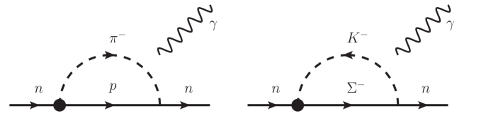
Figure 1: Diagrams which give rise to the neutron EDM. Solid, dashed, and wavy lines represent baryons, mesons, and photon, respectively. Further, dots indicate the CP-odd interactions given in Eqs. (22) and (23).

By using the interactions obtained above, we now evaluate the neutron EDM. It is induced by the diagrams displayed in Fig. 1. Here, solid, dashed, and wavy lines represent baryons, mesons, and photon, respectively. Further, dots indicate the CP-odd interactions given in Eqs. (22) and (23). The resultant formula for the neutron EDM is as follows:

$$d_{n}=-\frac{e}{4\sqrt{2}\pi^{2}f_{\pi}}\biggl{[}(D+F)\overline{g}_{pn\pi}\log\biggl{(}\frac{\Lambda}{m_{\pi}}\biggr{)}-(D-F)\overline{g}_{\Sigma nK}\log\biggl{(}\frac{\Lambda}{m_{K}}\biggr{)}\biggr{]}~{},$$ (50)

with $m_{\pi}$ and $m_{K}$ the masses of pion and kaon, respectively. Here, we extract the terms which contain logarithmic singularities in the chiral limit. $\Lambda\simeq M_{\rm B}$ is a UV cutoff. Furthermore, there exists tree-level, higher order contribution which acts as counterterms [21]. With the contribution added to the above equation, we obtain scale-independent formula for the neutron EDM. However, the low-energy constants for the operators which give rise to the tree-level contribution are not determined through the symmetry arguments. Thus, these unknown factors as well as the lack of other non-singular terms in Eq. (50) result in theoretical uncertainty. In the following calculation, we just directly use the expression (50) with $\Lambda$ taken to be the proton mass as an approximation. Note that the size of $\log(\Lambda/m_{K})$ is not large enough and thus might be considerably suffered from the uncertainty coming from the counterterms. The error originating from the approximation is to be estimated by varying the cutoff scale, similar to Ref. [21].

4 Evaluation of $S_{q}$ and $D_{q}$

Now all we have to do is to evaluate the proton matrix elements, $S_{q}$ and $D_{q}$.

4.1 $S_{q}$

As we mentioned in the Introduction, $S_{q}$ is directly extracted from the lattice QCD simulations. To evaluate them, we first introduce the following parameters:

$$\sigma_{\pi N} = \frac{m_{u}+m_{d}}{2}\langle p|\bar{u}u+\bar{d}d|p\rangle\ ,$$

$$\sigma_{s} = {m_{s}}\langle p|\bar{s}s|p\rangle\ ,$$

$$\xi = \frac{\langle p|\bar{u}u-\bar{d}d|p\rangle}{\langle p|\bar{u}u+\bar{d}d|p\rangle}\ .$$ (51)

Exploiting these parameters, we express $S_{q}$ as

$$S_{u} =\frac{1}{2}\frac{2}{(m_{u}+m_{d})}(1+\xi)\sigma_{\pi N},~{}$$

$$S_{d} =\frac{1}{2}\frac{2}{(m_{u}+m_{d})}(1-\xi)\sigma_{\pi N},~{}$$

$$S_{s} =\frac{\sigma_{s}}{m_{s}}.$$ (52)

Recent lattice simulations predict [37, 38]

$$\sigma_{\pi N} =45\pm 6~{}{\rm MeV},$$

$$\sigma_{s} =21\pm 6~{}{\rm MeV}.$$ (53)

The symmetry breaking parameter $\xi$ is obtained from the baryon mass splittings as [39]

$$\xi =\frac{m_{\Xi^{0}}+m_{\Xi^{-}}-m_{\Sigma^{+}}-m_{\Sigma^{-}}}{m_{\Xi^{0}}+m_{\Xi^{-}}+m_{\Sigma^{+}}+m_{\Sigma^{-}}-2m_{p}-2m_{n}}\biggl{(}1-\frac{m_{u}+m_{d}}{2m_{s}}\frac{2\sigma_{s}}{\sigma_{\pi N}}\biggr{)}$$

$$=0.197\biggl{(}1-\frac{m_{u}+m_{d}}{2m_{s}}\frac{2\sigma_{s}}{\sigma_{\pi N}}\biggr{)}~{}.$$ (54)

Then, with the quark-mass parameters [33]

$$\frac{m_{u}+m_{d}}{2}=4.6\pm 0.7~{}{\rm MeV},~{}~{}~{}~{}~{}~{}m_{s}=115\pm 6~{}{\rm MeV},$$ (55)

we obtain the values of $S_{q}$ as

$$S_{u} =5.8,~{}~{}~{}~{}~{}~{}S_{d}=4.0,~{}~{}~{}~{}~{}~{}S_{s}=0.18.$$ (56)

Here, we evolve the masses of light quarks from the scale $\mu=2~{}{\rm GeV}$ to $\mu=1~{}{\rm GeV}$ by using the renormalization group equations. Note that the values of $S_{u}$ and $S_{d}$ are almost as twice as those in Ref. [25]. This is mainly due to the quark-mass parameters. Moreover, $S_{s}$ is much smaller than that in Ref. [25], since recent lattice simulations predict relatively small values for $\sigma_{s}$. This fact drives us to reevaluate the strange quark contribution to the neutron EDM, as we mentioned to in the Introduction.

4.2 $D_{q}$

For the values of $D_{q}$, on the other hand, we are not able to use the lattice simulations at the present time. Although it is desirable that the lattice simulations eventually determine $D_{q}$, for the time being, we evaluate them by using the method of QCD sum rules [5, 6]. A similar approach is studied in Ref. [32].

For this purpose, we first add to the ordinary QCD Lagrangian the following terms which couple to the external $c$-number fields $J_{q}$:

$${\cal L}_{\rm ext}=J_{q}\bar{q}g_{s}G\cdot\sigma q~{}.$$ (57)

The method of QCD sum rules requires that we evaluate the correlation function of the proton interpolating fields in terms of two different ways; one is to describe it from the phenomenological point of view, and the other is to calculate it in terms of the operator product expansion (OPE). The correlation function we are to evaluate is defined as follows:

$$\Pi(k)|_{J}\equiv i\int d^{4}xe^{ik\cdot x}\langle\Omega|T\{\eta_{p}(x),\overline{\eta}_{p}(0)\}|\Omega\rangle_{J}~{},$$ (58)

with $\eta_{p}(x)$ the interpolating field for proton. The subscript of the correlator, $J$, indicates that the function in Eq. (58) is evaluated in the presence of external fields. We expand the correlation function in terms of $J_{q}$ as

$$\Pi(k)|_{J}=\Pi^{0}(k)+J_{q}\Pi_{q}(k)+{\cal O}(J^{2}),$$ (59)

and focus on the correlator $\Pi_{q}$ since it includes information on $D_{q}$.

The matrix element of the proton interpolating field between the vacuum and the one-particle proton state is given as

$$\langle\Omega|\eta_{p}(x)|p(\bm{k},s)\rangle=\frac{\lambda_{p}}{\sqrt{2m_{p}}}u_{p}(\bm{k},s)e^{-ik\cdot x}~{}.$$ (60)

Here, $u_{p}(\bm{k},s)$ is a spinor wave function, which is normalized as usual, i.e., $\bar{u}(\bm{k},s^{\prime})u(\bm{k},s)=2m_{p}\delta_{ss^{\prime}}$. We parametrize the field renormalization constant as $\lambda_{p}$, whose value is to be determined later.

A phenomenological description of the correlator is readily given as

$$\Pi_{q}(k)=\lambda_{p}^{2}D_{q}\frac{1}{{\ooalign{\hfil/\hfil\crcr$k$}}-m_{p}}\frac{1}{{\ooalign{\hfil/\hfil\crcr$k$}}-m_{p}}+\dots~{},$$ (65)

where the dots indicate the contribution of the excited states. Among the terms in the above expression, we hereafter focus on the terms that contain only one gamma matrix, that is, the terms proportional to / $k$ . Then, it follows that

$$\Pi_{q}(k)={\ooalign{\hfil/\hfil\crcr$k$}}f_{q}(k^{2})+\dots~{},$$ (68)

with

$$f_{q}(k^{2})\equiv\frac{2m_{p}\lambda_{p}^{2}D_{q}}{(k^{2}-m_{p}^{2})^{2}}+\frac{A_{q}(k^{2})}{k^{2}-m_{p}^{2}}+B_{q}(k^{2})~{}.$$ (69)

Here, $A_{q}(k^{2})$ and $B_{q}(k^{2})$ are the functions that have no pole at $k^{2}=m_{p}^{2}$. Dots in Eq. (68) correspond to terms with no gamma matrices.

In order to evaluate the correlation function by using the OPE, on the other hand, one needs to express the proton interpolating field in terms of a composite operator of quarks which has the same quantum numbers as those of a proton. The general form of the proton interpolating field is given as

$$\eta_{p}(x)=j_{p1}(x)+\beta j_{p2}(x)~{},$$ (70)

where

$$j_{p1}(x) \equiv 2\epsilon^{abc}[u^{T}_{a}(x)C\gamma_{5}d_{b}(x)]u_{c}(x),$$

$$j_{p2}(x) \equiv 2\epsilon^{abc}[u^{T}_{a}(x)Cd_{b}(x)]\gamma_{5}u_{c}(x).$$ (71)

Here the subscripts, $a,b,c$, are the color indices and $C$ denotes the charge conjugation matrix. Although the interpolator $j_{p2}(x)$ vanishes in the non-relativistic limit, there is no reason for the interpolator to be excluded since light quarks in a proton are actually relativistic. The unphysical parameter $\beta$ is to be fixed later. The OPE calculation is conducted with the quark propagators and condensates in the presence of the external fields. They are derived in Appendix B. By using them, we evaluate the correlation function and extract the terms proportional to the external fields. First, we decompose the correlation function as

$$\Pi(x)|_{J} =\langle\Omega|T\{\eta_{p}(x)\bar{\eta}_{p}(0)\}|\Omega\rangle_{J}$$

$$=\langle\Omega|T\{j_{p1}(x)\bar{j}_{p1}(0)\}|\Omega\rangle_{J}+\beta\{\langle\Omega|T\{j_{p2}(x)\bar{j}_{p1}(0)\}|\Omega\rangle_{J}$$

$$~{}~{}~{}~{}~{}~{}~{}~{}~{}~{}~{}~{}~{}+\langle\Omega|T\{j_{p1}(x)\bar{j}_{p2}(0)\}|\Omega\rangle_{J}\}+\beta^{2}\langle\Omega|T\{j_{p2}(x)\bar{j}_{p2}(0)\}|\Omega\rangle_{J}~{}.$$ (72)

For convenience, we use the following abbreviation:

$$\Pi_{kl}(x)=\langle\Omega|T\{j_{pk}(x)\bar{j}_{pl}(0)\}|\Omega\rangle~{},~{}~{}~{}~{}~{}~{}(k,l=1,2)~{}.$$ (73)

They are expressed in terms of the propagators $S^{q}_{ab}(x)$ given in Eq. (109) in Appendix. B as follows:

$$\Pi_{11}(x) =4\epsilon_{abc}\epsilon_{a^{\prime}b^{\prime}c^{\prime}}\bigl{[}{\rm Tr}\{\overline{S}^{u}_{aa^{\prime}}(x)\gamma_{5}S^{d}_{bb^{\prime}}(x)\gamma_{5}\}S^{u}_{cc^{\prime}}(x)+S^{u}_{aa^{\prime}}(x)\gamma_{5}\overline{S}^{d}_{bb^{\prime}}(x)\gamma_{5}S^{u}_{cc^{\prime}}(x)\bigr{]},$$

$$\Pi_{12}(x) =4\epsilon_{abc}\epsilon_{a^{\prime}b^{\prime}c^{\prime}}\bigl{[}{\rm Tr}\{\overline{S}^{u}_{aa^{\prime}}(x)\gamma_{5}S^{d}_{bb^{\prime}}(x)\}S^{u}_{cc^{\prime}}(x)\gamma_{5}+S^{u}_{aa^{\prime}}(x)\overline{S}^{d}_{bb^{\prime}}(x)\gamma_{5}S^{u}_{cc^{\prime}}(x)\gamma_{5}\bigr{]},$$

$$\Pi_{21}(x) =4\epsilon_{abc}\epsilon_{a^{\prime}b^{\prime}c^{\prime}}\bigl{[}{\rm Tr}\{\gamma_{5}\overline{S}^{u}_{aa^{\prime}}(x)S^{d}_{bb^{\prime}}(x)\}\gamma_{5}S^{u}_{cc^{\prime}}(x)+\gamma_{5}S^{u}_{aa^{\prime}}(x)\gamma_{5}\overline{S}^{d}_{bb^{\prime}}(x)S^{u}_{cc^{\prime}}(x)\bigr{]},$$

$$\Pi_{22}(x) =4\epsilon_{abc}\epsilon_{a^{\prime}b^{\prime}c^{\prime}}\bigl{[}{\rm Tr}\{\overline{S}^{u}_{aa^{\prime}}(x)S^{d}_{bb^{\prime}}(x)\}\gamma_{5}S^{u}_{cc^{\prime}}(x)\gamma_{5}+\gamma_{5}S^{u}_{aa^{\prime}}(x)\overline{S}^{d}_{bb^{\prime}}(x)S^{u}_{cc^{\prime}}(x)\gamma_{5}\bigr{]},$$ (74)

where

$$\overline{S}^{q}_{ab}(x)\equiv CS^{qT}_{ab}(x)C^{\dagger}.$$ (75)

Then, a series of Wick contraction leads to

$$\Pi_{11}(x)|_{J} =-\frac{i}{8\pi^{4}}\langle\bar{q}q\rangle\frac{{\ooalign{\hfil/\hfil\crcr$x$}}}{(x^{2})^{3}}(9J_{u}+5J_{d})m_{0}^{2},$$ (78)

$$\Pi_{12}(x)|_{J} =-\frac{i}{8\pi^{4}}\langle\bar{q}q\rangle\frac{{\ooalign{\hfil/\hfil\crcr$x$}}}{(x^{2})^{3}}(3J_{u}+J_{d})m_{0}^{2},$$ (81)

$$\Pi_{21}(x)|_{J} =-\frac{i}{8\pi^{4}}\langle\bar{q}q\rangle\frac{{\ooalign{\hfil/\hfil\crcr$x$}}}{(x^{2})^{3}}(3J_{u}+J_{d})m_{0}^{2},$$ (84)

$$\Pi_{22}(x)|_{J} =-\frac{i}{8\pi^{4}}\langle\bar{q}q\rangle\frac{{\ooalign{\hfil/\hfil\crcr$x$}}}{(x^{2})^{3}}(9J_{u}+5J_{d})m_{0}^{2},$$ (87)

up to the leading order. Here, we keep only the terms including an external field. It is followed that

$$\Pi(x)|_{J}=-\frac{i}{8\pi^{4}}\langle\bar{q}q\rangle\frac{{\ooalign{\hfil/\hfil\crcr$x$}}}{(x^{2})^{3}}m_{0}^{2}\bigl{[}(9\beta^{2}+6\beta+9)J_{u}+(5\beta^{2}+2\beta+5)J_{d}\bigr{]},$$ (90)

and its Fourier transformation results in

$$\Pi(k)|_{J}=-\frac{1}{32\pi^{2}}\langle\bar{q}q\rangle{\ooalign{\hfil/\hfil\crcr$k$}}\log\biggl{(}\frac{-k^{2}}{\Lambda^{2}}\biggr{)}m^{2}_{0}\bigl{[}(9\beta^{2}+6\beta+9)J_{u}+(5\beta^{2}+2\beta+5)J_{d}\bigr{]},$$ (93)

with $\Lambda$ a certain ultraviolet mass scale.

Then, by applying the Borel transformation to Eqs. (68) and (93), we now obtain the sum rules for $D_{q}$ as

$$D_{u}-\frac{A_{u}}{2m_{p}\lambda_{p}^{2}}M^{2} =+\frac{M^{4}}{32\pi^{2}}\frac{\langle\bar{q}q\rangle}{2m_{p}\lambda_{p}^{2}}\exp\biggl{\{}\frac{m_{p}^{2}}{M^{2}}\biggr{\}}(9\beta^{2}+6\beta+9)m^{2}_{0},$$

$$D_{d}-\frac{A_{d}}{2m_{p}\lambda_{p}^{2}}M^{2} =+\frac{M^{4}}{32\pi^{2}}\frac{\langle\bar{q}q\rangle}{2m_{p}\lambda_{p}^{2}}\exp\biggl{\{}\frac{m_{p}^{2}}{M^{2}}\biggr{\}}(5\beta^{2}+2\beta+5)m_{0}^{2},$$ (94)

and $D_{s}=0$ up to the leading order calculation. When we drive the sum rules, we assume that the single-pole contributions $A_{q}$ scarcely depend on $k^{2}$ around $k^{2}=m_{p}^{2}$, and regard them as constants. Further, we just neglect $B_{q}$ with expecting that their contributions are sufficiently reduced by the Borel transformation. Note that the sum rules in Eq. (94) contain the identical function of $M^{2}$, $M^{4}\exp(m_{p}^{2}/M^{2})$, in their right-hand side. Moreover, the tangent line to the function at a given Borel mass squared $M^{2}$ gives us both the first and second terms in the left-hand side of the sum rules [14]. Especially, if one sets the Borel mass at the minimal of the function, i.e., $M^{2}=m_{p}^{2}/2$, the single-pole contributions vanish. Since this choice also makes the sum rules stable under the slight variation of the Borel mass, we adopt it in the following discussion.

Now all we have to do reduces to the determination of the constant $\lambda_{p}$. One way to evaluate it is again using the method of QCD sum rules. In Ref. [40], two sum rules which allow us to extract $\lambda_{p}$ are presented; one contains the Lorentz structure / $p$ and the other is proportional to unity. On the other hand, it is possible to extract the value from the lattice result. By using the parameters obtained in Ref. [41], we obtain

$$\lambda_{p}=2\times 0.91\cdot\bigl{[}(\alpha_{1}-\alpha_{2})-\beta(\alpha_{1}+\alpha_{2})\bigr{]}~{},$$ (95)

with the parameters $\alpha_{1}$ and $\alpha_{2}$ given as

$$\alpha_{1}=-0.0112\pm 0.0012_{(\rm stat)}\pm 0.0022_{(\rm syst)}~{}{\rm GeV}^{3}~{},$$

$$\alpha_{2}=0.0120\pm 0.0013_{(\rm stat)}\pm 0.0023_{(\rm syst)}~{}{\rm GeV}^{3}~{}.$$ (96)

Here we take the renormalization effect into account [14]. These values are consistent with those obtained by another group [42] within the errors of their simulations. In the following calculation, we use the values for $\lambda_{p}$ evaluated in both approaches, and present two results corresponding to these two values.

The estimation of $D_{q}$ presented here is, however, to be considered as just for reference. At the moment we only present center values for those quantity. In order to estimate the theoretical error for the calculation and to improve the accuracy of the result, we need the investigation of the excited/continuum state contribution as well as the execution of the higher order calculation for the OPE. In the higher order calculation, there exist several unknown condensates such as the susceptibilities of $\langle\bar{q}q\rangle$ with respect to the external sources, and thus they make it difficult to give a precise prediction. Therefore, much detail analysis with the determination of these unknown condensates is required for a robust calculation of $D_{q}$. We hope our study presented in this paper stimulates a lot of efforts to evaluate the quantity with various methods, especially with the lattice QCD simulations.

5 Results

Now we derive a relation between the neutron EDM with the CP-violating parameters by using the nucleon matrix elements obtained above. We use the values in Eq. (56) for $S_{q}$, while $D_{q}$ ($q=u,d$) are evaluated from the sum rules in Eq. (94) with $D_{s}$ presumed to be zero.

We are interested in the significance of the strange CEDM contribution to the neutron EDM. In order to examine it, we consider each contribution of CEDM in the presence of PQ symmetry. In this case, the resultant relation between the CEDMs and the neutron EDM is expressed as

$$d_{n}|_{\rm PQ}=\sum_{q}eC_{q}\frac{\tilde{d}_{q}}{m_{q}}.$$ (97)

Here, we normalize the CEDMs by the quark masses, since in most cases the quark CEDMs are proportional to the quark masses, $\tilde{d}_{q}\propto m_{q}$. Then, we look into the ratio of the coefficient $C_{s}$ against those of up and down quarks. It allows us to evade an overall factor of uncertainty coming from the logarithmic factor in Eq. (50), though the relative values of $C_{q}$ still might be affected.

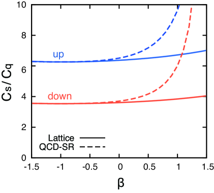
Figure 2: Ratios $C_{s}/C_{q}$ ($q=u,d$) as functions of the parameter $\beta$ in the sum rules. Upper blue (lower orange) lines show $C_{s}/C_{u}$ ($C_{s}/C_{d}$). Solid lines correspond to the results where we use $\lambda_{p}$ in Eq. (95), while dashed lines represent those obtained with $\lambda_{p}$ evaluated in Ref. [40].

In Fig. 2, we plot the ratios $C_{s}/C_{q}$ as functions of the parameter $\beta$ in the sum rules. The upper blue and the lower orange lines show $C_{s}/C_{u}$ and $C_{s}/C_{d}$, respectively. The solid lines correspond to the results in which we use $\lambda_{p}$ in Eq. (95), while the dashed lines represent those obtained with $\lambda_{p}$ evaluated in Ref. [40]. In the calculation, we take $m_{0}^{2}=0.8~{}{\rm GeV}^{2}$ [31] and $\langle\bar{q}q\rangle$ is evaluated using the relation $\langle\bar{q}q\rangle=-m_{\pi}^{2}f_{\pi}^{2}/(m_{u}+m_{d})$ as $\langle\bar{q}q\rangle\simeq-(262~{}{\rm MeV})^{3}$ at the scale of $\mu=1~{}{\rm GeV}$. In addition, when we compute $\lambda_{p}$ from the results in Ref. [40], we use the sum rule for / $p$ and set the threshold $w$ and the gluon condensate $b\equiv(2\pi)^{2}(\frac{\alpha_{s}}{\pi}GG)$ as $w=2~{}{\rm GeV}$ and $b=470~{}{\rm MeV}^{4}$, respectively. With the parameters we obtain $|\lambda_{p}|\simeq 0.04~{}{\rm GeV}^{3}$ for $\beta=-1$ and $|\lambda_{p}|\simeq 0.02~{}{\rm GeV}^{3}$ for $\beta=+1$. It is found that both calculations for $\lambda_{p}$ give rise to similar results in the case of $\beta\lesssim 0$, while one deviates form the other for positive $\beta$. In any case, the strange CEDM contribution is sizable, in fact dominates the other contributions, though the strangeness content of nucleon is quite small. The contribution comes from the $K$-meson loop and does not vanish in the limit of small $S_{s}$ and $D_{s}$, as it is understood from Eq. (25).

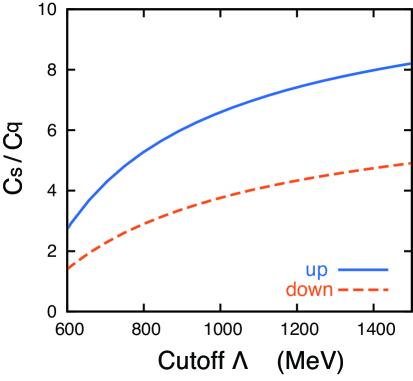
Figure 3: Dependence of $C_{s}/C_{q}$ on cutoff scale $\Lambda$. Blue solid and orange dashed lines show the results for up and down quarks, respectively. We use $\lambda_{p}$ with $\beta=-1$ in Eq. (95) in the calculation.

As we have mentioned to above, the computation suffers from the uncertainty due to the tree-level contribution of the unknown counterterms as well as the lack of other non-singular terms in Eq. (50). To estimate its significance, we vary the cutoff scale $\Lambda$ in Eq. (50), following the analysis in Ref. [12]. In Fig. 3, we plot the dependence of the ratios $C_{s}/C_{q}$ on $\Lambda$. The blue solid (orange dashed) line shows the result for $C_{s}/C_{u}$ ($C_{s}/C_{d}$). We use the lattice result in Eq. (95) for the value of $\lambda_{p}$ with $\beta$ set to be $-1$. This figure tells us that although the variation of the cutoff scale may change the ratio by an ${\cal O}(1)$ factor, the contribution of strange CEDM tends to remain important. Taking the results obtained above into consideration, we conclude that although the recent lattice results indicate that the amount of strange quark in nucleon is small, the CEDM of strange quark may play an important role in probing the CP-violating interactions in physics beyond the SM with the neutron EDM.

Finally, as a reference value, we present the numerical results for the relation between the CEDMs and the neutron EDM:

$$d_{n}=e(5.8\times 10^{-16}\bar{\theta}~{}[{\rm cm}]-1.4\tilde{d}_{u}+0.7\tilde{d}_{d}+0.4\tilde{d}_{s}),$$ (98)

where we take $\beta=-1$ and use $\lambda_{p}$ in Eq. (95). Note that unlike the CEDM contribution, the calculation of the $\bar{\theta}$ contribution is not affected by the uncertainty in the values of $D_{q}$, since the contribution only depends on $S_{q}$. In this sense, the result for the $\bar{\theta}$ contribution to the neutron EDM is robust up to the uncertainty coming from the chiral loop calculation. In the presence of the PQ symmetry, on the other hand, the relation is modified to

$$d_{n}|_{\rm PQ}=e(3.0\tilde{d}_{u}+2.5\tilde{d}_{d}+0.5\tilde{d}_{s}).$$ (99)

Here, we would like to remark that there may be large error in estimating the size of the strange CEDM contribution, which results from the uncertainty of the kaon-loop contribution discussed in Sec. 3. For instance, if we take $\Lambda$ to be the $\rho$-meson mass, the strangeness contribution is found to be suppressed by 30 %, while with $\Lambda=m_{\Sigma}$, it is enhanced by about 40 %. Hence, much detailed analyses of the chiral-loop contributions as well as the estimate of the tree-level counterterms are required in order to reduce the uncertainty.

Compared to the results obtained with the QCD sum rules [12, 14], our results here predict relatively large neutron EDM. Indeed, a latest calculation conducted in Ref. [14] gives

$$d_{n}=e(8.2\times 10^{-17}\bar{\theta}~{}[{\rm cm}]-0.30\tilde{d}_{u}+0.30\tilde{d}_{d}-0.01\tilde{d}_{s}),$$ (100)

and in the presence of the PQ symmetry, it reduces to

$$d_{n}|_{\rm PQ}=e(0.30\tilde{d}_{u}+0.59\tilde{d}_{d}).$$ (101)

These values are found to be smaller than ours by ${\cal O}(1)$ factors. The expression tells us that the strangeness contribution vanishes when you exploit the method of QCD sum rules, where the sea quark effects show up only at the higher orders. The same consequence is obtained if you use the results in Ref. [12]. With the present knowledge, we are not able to conclude which method is appropriate for the calculation of the neutron EDM, since both of them may have substantial uncertainty.

6 Conclusion

We have calculated the neutron electric dipole moment in the presence of the CP-violating operators up to dimension five based on the chiral perturbation theory. In the calculation, we extract the nucleon matrix elements of scalar-type quark operators, $S_{q}$, from the recent lattice results, while those of the dipole-type quark-gluon operators, $D_{q}$, are evaluated by using the method of the QCD sum rules. Especially, we focus on the strange CEDM contribution to the neutron EDM. Although the lattice QCD simulations tell us that the strangeness content in nucleon is small, it is found the contribution may not be suppressed.

There are two origins of the theoretical error in our calculation; one is unknown counterterms in the effective Lagrangian which contribute to the neutron EDM at tree level, and the other is the evaluation of $D_{q}$ by using the method of QCD sum rules. The former is somewhat inevitable until one fixes all of the low-energy constants for the counterterms. The latter is, on the other hand, expected to be improved if the higher order calculation is conducted with unknown condensates determined from other studies. Further, the lattice QCD simulations might compute $D_{q}$ directly. It allows us to make a prediction of neutron EDM much precisely with error estimated more systematically.

At present, we conclude that the contribution of strange quark CEDM may be still significant, and therefore it might offer a sensitive probe for the CP-violating interactions in physics beyond the Standard Model.

Appendix

Appendix A Baryon matrix elements

In this section, we derive formulae for the baryon matrix elements given in Eq. (19). To that end, we first rewrite ${\cal A}$ in terms of the SU(3) generators:

$${\cal A}=\frac{1}{3}({\cal A}_{u}+{\cal A}_{d}+{\cal A}_{s})\mbox{1}\mbox{l}+({\cal A}_{u}-{\cal A}_{d})T^{3}+\frac{1}{\sqrt{3}}({\cal A}_{u}+{\cal A}_{d}-2{\cal A}_{s})T^{8}~{}.$$ (102)

Then, by using the anticommuting relations

$$\{T^{A},T^{B}\}=\frac{1}{3}\delta_{AB}+d_{ABC}T^{C}~{},$$ (103)

we obtain

$$\langle B^{B} |\overline{Q}\{T^{A},{\cal A}\}Q|B^{C}\rangle$$

$$=\frac{2}{3}\langle B^{B}|\overline{Q}({\cal A}_{u}+{\cal A}_{d}+{\cal A}_{s})T^{A}Q|B^{C}\rangle+\frac{1}{3}\delta_{A3}\langle B^{B}|\overline{Q}({\cal A}_{u}-{\cal A}_{d})Q|B^{C}\rangle$$

$$+d_{A3D}\langle B^{B}|\overline{Q}({\cal A}_{u}-{\cal A}_{d})T^{D}Q|B^{C}\rangle+\frac{1}{3\sqrt{3}}\delta_{A8}\langle B^{B}|\overline{Q}({\cal A}_{u}+{\cal A}_{d}-2{\cal A}_{s})Q|B^{C}\rangle$$

$$+\frac{1}{\sqrt{3}}d_{A8D}\langle B^{B}|\overline{Q}({\cal A}_{u}+{\cal A}_{d}-2{\cal A}_{s})T^{D}Q|B^{C}\rangle~{}.$$ (104)

Here, we define $d_{ABC}$ as $d_{ABC}\equiv 2{\rm Tr}[\{T^{A},T^{B}\}T^{C}]$.

Next, we express the baryon matrix elements in the above equation in terms of the baryon matrix field $B$ defined in Eq. (32). Since there are two different ways of combining three matrices to form an SU(3) covariant form, we parametrize the baryon matrix elements as

$$\langle B^{B}|\overline{Q}({\cal A}_{u}+{\cal A}_{d}+{\cal A}_{s})T^{A}Q|B^{C}\rangle\overline{B^{B}}B^{C} \equiv X_{1}{\rm Tr}(\overline{B}T^{A}B)+Y_{1}{\rm Tr}(\overline{B}BT^{A})~{},$$

$$\langle B^{B}|\overline{Q}({\cal A}_{u}-{\cal A}_{d})T^{A}Q|B^{C}\rangle\overline{B^{B}}B^{C} \equiv X_{3}{\rm Tr}(\overline{B}T^{A}B)+Y_{3}{\rm Tr}(\overline{B}BT^{A})~{},$$

$$\langle B^{B}|\overline{Q}({\cal A}_{u}+{\cal A}_{d}-2{\cal A}_{s})T^{A}Q|B^{C}\rangle\overline{B^{B}}B^{C} \equiv X_{8}{\rm Tr}(\overline{B}T^{A}B)+Y_{8}{\rm Tr}(\overline{B}BT^{A})~{}.$$ (105)

Further, considering the combination of two matrices to form an $SU(3)$ singlet, we obtain

$$\langle B^{B}|\overline{Q}({\cal A}_{u}-{\cal A}_{d})Q|B^{C}\rangle\overline{B^{B}}B^{C} \equiv Z_{3}{\rm Tr}(\overline{B}B)~{},$$

$$\langle B^{B}|\overline{Q}({\cal A}_{u}+{\cal A}_{d}-2{\cal A}_{s})Q|B^{C}\rangle\overline{B^{B}}B^{C} \equiv Z_{8}{\rm Tr}(\overline{B}B)~{}.$$ (106)

These parameters can be written in terms of proton matrix elements. Then, using $S_{q}$ and $D_{q}$ defined in Eq.(20), we express the parameters in Eqs. (105) and (106) as

$$X_{1} =-(m_{u}\theta_{u}+m_{d}\theta_{d}+m_{s}\theta_{s})(S_{u}-S_{d})-\frac{1}{2}(\tilde{d}_{u}+\tilde{d}_{d}+\tilde{d}_{s})(D_{u}-D_{d})~{},$$

$$X_{3} =-(m_{u}\theta_{u}-m_{d}\theta_{d})(S_{u}-S_{d})-\frac{1}{2}(\tilde{d}_{u}-\tilde{d}_{d})(D_{u}-D_{d})~{},$$

$$X_{8} =-(m_{u}\theta_{u}+m_{d}\theta_{d}-2m_{s}\theta_{s})(S_{u}-S_{d})-\frac{1}{2}(\tilde{d}_{u}+\tilde{d}_{d}-2\tilde{d}_{s})(D_{u}-D_{d})~{},$$

$$Y_{1} =-(m_{u}\theta_{u}+m_{d}\theta_{d}+m_{s}\theta_{s})(S_{s}-S_{d})-\frac{1}{2}(\tilde{d}_{u}+\tilde{d}_{d}+\tilde{d}_{s})(D_{s}-D_{d})~{},$$

$$Y_{3} =-(m_{u}\theta_{u}-m_{d}\theta_{d})(S_{s}-S_{d})-\frac{1}{2}(\tilde{d}_{u}-\tilde{d}_{d})(D_{s}-D_{d})~{},$$

$$Y_{8} =-(m_{u}\theta_{u}+m_{d}\theta_{d}-2m_{s}\theta_{s})(S_{s}-S_{d})-\frac{1}{2}(\tilde{d}_{u}+\tilde{d}_{d}-2\tilde{d}_{s})(D_{s}-D_{d})~{},$$

$$Z_{3} =-(m_{u}\theta_{u}-m_{d}\theta_{d})(S_{u}+S_{d}+S_{s})-\frac{1}{2}(\tilde{d}_{u}-\tilde{d}_{d})(D_{u}+D_{d}+D_{s})~{},$$

$$Z_{8} =-(m_{u}\theta_{u}+m_{d}\theta_{d}-2m_{s}\theta_{s})(S_{u}+S_{d}+S_{s})-\frac{1}{2}(\tilde{d}_{u}+\tilde{d}_{d}-2\tilde{d}_{s})(D_{u}+D_{d}+D_{s})~{}.$$ (107)

Appendix B Quark propagators and correlators of the background fields

In the OPE calculation carried out in Sec. 4.2, we need to obtain the quark propagators as well as the correlators of the quark/gluon background fields in the presence of the interaction in Eq. (57). The quark propagators are defined as follows:

$$[S^{q}_{ab}(x)]_{\alpha\beta}\equiv\langle\Omega|T\left[q_{a\alpha}(x)\bar{q}_{b\beta}(0)\right]|\Omega\rangle_{J}~{},$$ (108)

where $\alpha$ and $\beta$ denote spinor indices. Furthermore, we perturbatively expand the propagators as

$$\left[S^{q}_{ab}(x)\right]_{\alpha\beta}=\left[S^{q(0)}_{ab}(x)\right]_{\alpha\beta}+\chi^{q}_{a\alpha}(x)\bar{\chi}^{q}_{b\beta}(0)+\left[S^{q}_{ab}(x)\right]_{\alpha\beta}|_{g}+\dots~{}.$$ (109)

The first term is the free propagator, and the second term describes the correlator of the quark background fields, with $\chi^{q}_{a\alpha}(x)$ a classical Grassmann field which indicates the quark background field. The third term represents the propagator which includes one gluon. Let us evaluate these terms in $x$-space. The first term, $[S^{q(0)}_{ab}(x)]_{\alpha\beta}$, is readily evaluated as

$$S^{q(0)}_{ab}(x) =\frac{i\delta_{ab}}{2\pi^{2}}\frac{{\ooalign{\hfil/\hfil\crcr$x$}}}{(x^{2})^{2}},$$ (112)

where we neglect the quark masses since their contribution only appears in the higher order operators.

Next, we evaluate the third term in Eq. (109). In this calculation, it is convenient to exploit the Fock-Schwinger gauge [44] for the gluon field. In this gauge, the gluon field is subjected to the following gauge fixing condition:

$$x^{\mu}G_{\mu}(x)=0~{},$$ (113)

where $G_{\mu}(x)\equiv G^{A}_{\mu}(x)T^{A}$ is the gluon field. Then, it is expanded by its field strength tensor such that

$$G_{\mu}(x)=\frac{1}{2\cdot 0!}x^{\nu}G_{\nu\mu}(0)+\frac{1}{3\cdot 1!}x^{\alpha}x^{\nu}(D_{\alpha}G_{\nu\mu}(0))+\frac{1}{4\cdot 2!}x^{\alpha}x^{\beta}x^{\nu}(D_{\alpha}D_{\beta}G_{\nu\mu}(0))+\cdots.$$ (114)

By using the expression, the gauge covariant form of the propagators is obtained as follows:

$$S^{q}_{ab}(x)|_{g}= -\frac{g_{s}}{32\pi^{2}}\biggl{[}\frac{i}{x^{2}}\{{\ooalign{\hfil/\hfil\crcr$x$}},G_{ab}\cdot\sigma\}+4J_{q}\frac{{\ooalign{\hfil/\hfil\crcr$x$}}G_{ab}\cdot\sigma{\ooalign{\hfil/\hfil\crcr$x$}}}{(x^{2})^{2}}~{}\biggr{]},$$ (121)

with $G_{ab}^{\mu\nu}=G^{A\mu\nu}T^{A}_{ab}$. Here we keep only the first order terms with respect to the external fields, $J_{q}$.

Also, we translate the quark and gluon background fields into their condensates. The correlation function of quark background fields, $\chi^{q}_{a\alpha}(x)\bar{\chi}^{q}_{b\beta}(0)$, is related with the quark condensate as

$$\chi^{q}_{a\alpha}(x)\bar{\chi}^{q}_{b\beta}(0)=\langle\Omega|T[q_{a\alpha}(x)\bar{q}_{b\beta}(0)]|\Omega\rangle.$$ (122)

By using the Fierz identities and carrying out the short-distance expansion of the quark field,

$$q(x)=q(0)+x^{\mu}D_{\mu}q(0)+\dots~{},$$ (123)

we obtain

$$\chi^{q}_{a\alpha}(x)\bar{\chi}^{q}_{b\beta}(0)= -\frac{\delta_{ab}}{12}\langle\bar{q}q\rangle[\mbox{1}\mbox{l}-\frac{i}{4}{\ooalign{\hfil/\hfil\crcr$x$}}J_{q}m^{2}_{0}]_{\alpha\beta}~{}.$$ (126)

In general, the vacuum condensate in the presence of external fields, $\langle\bar{q}q\rangle|_{J}$, is different from ordinary one, $\langle\bar{q}q\rangle$[45]. However, the susceptibilities of the condensates to the external fields only appear in the higher order of the OPE, therefore, we neglect them since in our calculation we just deal with the leading order contributions.

In addition, we need the interaction part of the quark and gluon background fields,

$$g_{s}\chi^{q}_{a\alpha}(x)\bar{\chi}^{q}_{b\beta}(0)G_{\mu\nu}^{A}=\langle\Omega|T[g_{s}q_{a\alpha}(x)G_{\mu\nu}^{A}\bar{q}_{b\beta}(0)]|\Omega\rangle,$$ (127)

and it leads to the following equation:

$$g_{s}\chi^{q}_{a\alpha}(x)\bar{\chi}^{q}_{b\beta}(0)G_{\mu\nu}^{A}=\frac{1}{192}T^{A}_{ab}m_{0}^{2}\langle\bar{q}q\rangle(\sigma_{\mu\nu})_{\alpha\beta}.$$ (128)

References

- [1] T. Mannel and N. Uraltsev, Phys. Rev. D 85, 096002 (2012).
- [2] I. B. Khriplovich and A. R. Zhitnitsky, Phys. Lett. B 109, 490 (1982).
- [3] C. A. Baker, D. D. Doyle, P. Geltenbort, K. Green, M. G. D. van der Grinten, P. G. Harris, P. Iaydjiev and S. N. Ivanov et al., Phys. Rev. Lett. 97, 131801 (2006).
- [4] K. Bodek, S. .Kistryn, M. Kuzniak, J. Zejma, M. Burghoff, S. Knappe-Gruneberg, T. Sander-Thoemmes and A. Schnabel et al., arXiv:0806.4837 [nucl-ex].
- [5] M. A. Shifman, A. I. Vainshtein and V. I. Zakharov, Nucl. Phys. B 147, 385 (1979).
- [6] M. A. Shifman, A. I. Vainshtein and V. I. Zakharov, Nucl. Phys. B 147, 448 (1979).
- [7] I. I. Kogan and D. Wyler, Phys. Lett. B 274, 100 (1992).
- [8] X. -m. Jin and J. Tang, Phys. Rev. D 56, 5618 (1997).
- [9] M. Pospelov and A. Ritz, Phys. Rev. Lett. 83, 2526 (1999).
- [10] C. -T. Chan, E. M. Henley and T. Meissner, hep-ph/9905317.
- [11] M. Pospelov and A. Ritz, Nucl. Phys. B 573, 177 (2000).
- [12] M. Pospelov and A. Ritz, Phys. Rev. D 63, 073015 (2001).
- [13] S. Narison, Phys. Lett. B 666, 455 (2008).
- [14] J. Hisano, J. Y. Lee, N. Nagata and Y. Shimizu, Phys. Rev. D 85, 114044 (2012).
- [15] E. Shintani, S. Aoki, N. Ishizuka, K. Kanaya, Y. Kikukawa, Y. Kuramashi, M. Okawa and Y. Tanigchi et al., Phys. Rev. D 72, 014504 (2005).
- [16] F. Berruto, T. Blum, K. Orginos and A. Soni, Phys. Rev. D 73, 054509 (2006).
- [17] E. Shintani, S. Aoki, N. Ishizuka, K. Kanaya, Y. Kikukawa, Y. Kuramashi, M. Okawa and A. Ukawa et al., Phys. Rev. D 75, 034507 (2007).
- [18] E. Shintani, S. Aoki and Y. Kuramashi, Phys. Rev. D 78, 014503 (2008).
- [19] S. Aoki, R. Horsley, T. Izubuchi, Y. Nakamura, D. Pleiter, P. E. L. Rakow, G. Schierholz and J. Zanotti, arXiv:0808.1428 [hep-lat].
- [20] R. J. Crewther, P. Di Vecchia, G. Veneziano and E. Witten, Phys. Lett. B 88, 123 (1979) [Erratum-ibid. B 91, 487 (1980)].
- [21] A. Pich and E. de Rafael, Nucl. Phys. B 367, 313 (1991).
- [22] B. Borasoy, Phys. Rev. D 61, 114017 (2000).
- [23] K. Ottnad, B. Kubis, U. G. Meissner and F. K. Guo, Phys. Lett. B 687, 42 (2010).
- [24] F. -K. Guo and U. -G. Meißner, arXiv:1210.5887 [hep-ph].
- [25] J. Hisano and Y. Shimizu, Phys. Rev. D 70, 093001 (2004).
- [26] J. de Vries, R. G. E. Timmermans, E. Mereghetti and U. van Kolck, Phys. Lett. B 695, 268 (2011).
- [27] E. Mereghetti, J. de Vries, W. H. Hockings, C. M. Maekawa and U. van Kolck, Phys. Lett. B 696, 97 (2011).
- [28] R. D. Peccei and H. R. Quinn, Phys. Rev. Lett. 38, 1440 (1977).
- [29] J. M. Alarcon, L. S. Geng, J. M. Camalich and J. A. Oller, arXiv:1209.2870 [hep-ph].
- [30] J. Hisano, K. Tsumura and M. J. S. Yang, Phys. Lett. B 713 (2012) 473.
- [31] V. M. Belyaev and B. L. Ioffe, Sov. Phys. JETP 56, 493 (1982) [Zh. Eksp. Teor. Fiz. 83, 876 (1982)].
- [32] M. Pospelov, Phys. Lett. B 530, 123 (2002).
- [33] J. Beringer et al. (Particle Data Group), Phys. Rev. D86, 010001 (2012).
- [34] I. I. Y. Bigi and N. G. Uraltsev, Sov. Phys. JETP 73, 198 (1991).
- [35] M. Pospelov, Phys. Rev. D 58, 097703 (1998).
- [36] S. Y. Hsueh, D. Muller, J. Tang, R. Winston, G. Zapalac, E. C. Swallow, J. P. Berge and A. E. Brenner et al., Phys. Rev. D 38, 2056 (1988).
- [37] S. Aoki et al. [PACS-CS Collaboration], Phys. Rev. D 79, 034503 (2009).
- [38] P. E. Shanahan, A. W. Thomas and R. D. Young, arXiv:1205.5365 [nucl-th].
- [39] H. Y. Cheng, Phys. Lett. B 219, 347 (1989).
- [40] D. B. Leinweber, Annals Phys. 254, 328 (1997).
- [41] Y. Aoki et al. [RBC-UKQCD Collaboration], Phys. Rev. D 78, 054505 (2008).
- [42] V. M. Braun et al. [QCDSF Collaboration], Phys. Rev. D 79, 034504 (2009).
- [43] V. M. Khatsimovsky, I. B. Khriplovich and A. S. Yelkhovsky, Annals Phys. 186, 1 (1988).
- [44] V. A. Novikov, M. A. Shifman, A. I. Vainshtein and V. I. Zakharov, Fortsch. Phys. 32, 585 (1984).
- [45] X. -m. Jin, M. Nielsen and J. Pasupathy, Phys. Lett. B 314, 163 (1993).