Jet Power and Black Hole Spin: Testing an Empirical Relationship and Using it to Predict the Spins of Six Black Holes

Abstract

Using 5 GHz radio luminosity at light-curve maximum as a proxy for jet power and black-hole spin measurements obtained via the continuum-fitting method, Narayan & McClintock (2012) presented the first direct evidence for a relationship between jet power and black hole spin for four transient black-hole binaries. We test and confirm their empirical relationship using a fifth source, H1743–322, whose spin was recently measured. We show that this relationship is consistent with Fe-line spin measurements provided that the black hole spin axis is assumed to be aligned with the binary angular momentum axis. We also show that, during a major outburst of a black hole transient, the system reasonably approximates an X-ray standard candle. We further show, using the standard synchrotron bubble model, that the radio luminosity at light-curve maximum is a good proxy for jet kinetic energy. Thus, the observed tight correlation between radio power and black hole spin indicates a strong underlying link between mechanical jet power and black hole spin. Using the fitted correlation between radio power and spin for the above five calibration sources, we predict the spins of six other black holes in X-ray/radio transient systems with low-mass companions. Remarkably, these predicted spins are all relatively low, especially when compared to the high measured spins of black holes in persistent, wind-fed systems with massive companions.

1. Introduction

Jets are observed in diverse astrophysical systems and by objects spanning a wide range of mass: protoplanetary disks around newly birthed stars, through white dwarfs, neutron stars, stellar-mass black holes, and up to the supermassive black holes which power active galactic nuclei (Livio, 1999). However, despite a wealth of observational data, the mechanisms responsible for launching and powering these jets remain uncertain. In this work, we sharply focus on one particular class of jets, namely, impulsive ballistic jets produced during the brightest phase of outbursting black hole transients. This is an advantageous approach to the study of jets because black holes are the simplest astrophysical objects, and also because, as we will show, the jets we consider are produced at very nearly the same (Eddington-scaled) mass accretion rates.

In total, there are a few dozen transient X-ray binary systems that are known to contain black hole primaries (Remillard & McClintock, 2006; Özel et al., 2010). A representative black hole transient is active for about a year and then quiescent for years or decades before again becoming active. At peak flux, a typical system approaches its Eddington limit, and it therefore approximates a standard candle, as we show in Appendix A.

Based on radio monitoring data collected for several of these X-ray transients, it is clear that these systems are also radio transients. Their radio light curves, although of shorter duration, mimic the X-ray behavior in that they rise rapidly and decay relatively slowly (e.g., Shrader et al. 1994; Brocksopp et al. 2002, 2007). However, the peak radio luminosities (unlike the peak X-ray luminosities) vary widely. Narayan & McClintock 2012 (hereafter NM12) showed for a sample of four black hole transients that their peak 5 GHz radio luminosities ranged over a factor of $\approx 250$ while their X-ray luminosities were all quite similar. As we show in Section 3, if one corrects for relativistic beaming, then this range of luminosities is significantly increased to $\approx 700$ for $\Gamma=2$ and $\approx 1000$ for $\Gamma=5$.

Assuming that the peak radio luminosities of these four transient sources track the kinetic power of their transient ballistic jets – an assumption that we show to be reasonable in Appendix B – and using the values of their spins determined via the continuum-fitting method, NM12 reached their central conclusion: Jet power increases dramatically with increasing black hole spin $a_{*}$. This is the first evidence that jets are powered by black hole spin, an effect originally predicted by Blandford & Znajek (1977). NM12 found that jet power scales approximately as $a_{*}^{2}$ or $\Omega_{H}^{2}M^{2}$, where $\Omega_{H}$ is the angular velocity of the horizon. Such a scaling is expected theoretically (Blandford & Znajek, 1977; Tchekhovskoy et al., 2010).

Our result contrasts with an earlier study by Fender et al. (2010) in which no correlation was found between jet power and spin. The primary difference between the Fender et al. and NM12 studies is the different proxies used for jet power. Briefly, Fender et al. computed jet power using a model based on the radio luminosity, X-ray flux and the rise time of a radio flare event, whereas NM12 simply used the peak radio luminosity directly as a proxy for jet power. For a fuller discussion of the differences between the two studies, we refer the reader to Section 4 in NM12.

In this paper, we increase from four to five the sample of microquasars with spins measured via the continuum-fitting method and with good radio coverage during outburst. Specifically, we add to our sample H1743–322 whose primary is a slowly spinning black hole, $a_{*}=0.2\pm 0.3$ (Steiner et al., 2012). H1743–322 (hereafter H1743) is very similar to the microquasar XTE J1550–564 in its X-ray properties (McClintock et al., 2009) and in its display of pc-scale X-ray and radio jets (Corbel et al., 2005). Despite the complete absence of optical dynamical data – even the orbital period of H1743 is unknown – a kinematic model of the jets allowed a precise determination of the source distance $D=8.5\pm 0.8$ kpc and jet inclination angle $i=75\pm 3\arcdeg$, which in turn allowed the spin of this black hole to be measured via the continuum-fitting method (Steiner et al., 2012).

In Section 2, we present our jet model, and in Section 3, we use the spin and radio monitoring data for H1743 to test the NM12 correlation between jet power and spin. In Section 4, we first update this correlation by refitting the data for all five systems, i.e., the four NM12 sources plus H1743. Then, as our central objective, we use this correlation to predict the values of spin for the six black hole primaries in the following transient systems: GRS 1124-683 (Nova Mus 1991), GX 339–4, XTE J1720–318, XTE J1748-288, XTE J1859+226 and GS 2000+25. In Section 5, we compare the correlation based on continuum-fitting spin data to the available Fe-line spin measurements for four black hole transients. Finally, we discuss our results in Section 6 and offer our conclusions in Section 7.

In Appendix A, we validate our “standard candle” assumption (NM12) by showing that during major outbursts the systems we consider reach a substantial fraction of their Eddington limit, and in Appendix B we describe a simple synchrotron bubble model and demonstrate that the radio synchrotron flux density at light-curve maximum is a reasonable proxy for jet kinetic power.

2. The Jet Power Model

We model the bipolar radio jet as a symmetric pair of isotropically-emitting and optically-thin plasmoids expanding outward from the core source at a relativistic bulk velocity $\beta$. The ratio of observed to emitted flux density for each jet is

$$S_{\nu}/S_{\nu,0}=\delta^{3-\alpha},$$ (1)

where $\delta$ is the Doppler factor and $\alpha$ is the radio spectral index (Mirabel & Rodríguez, 1999). The Doppler factor of the brighter (approaching) jet is simply expressed in terms of $\beta$, the Lorentz factor $\Gamma$, and the jet inclination angle $i$:

$$\delta\equiv\left(\Gamma[1-\beta~{}{\rm cos}~{}i]\right)^{-1}.$$ (2)

For the dominant source of emission, i.e. the approaching jet, the observed intensity is greater than the emitted intensity for low inclinations, and conversely for high inclinations. For the mildly relativistic jets of microquasars, $2\lesssim\Gamma\lesssim 5$ (Fender et al., 2004; Fender, 2006), the Doppler boost becomes less than unity at intermediate values of inclination in the range $\approx 35-55\arcdeg$.

The NM12 model assumes that the full power of a black hole’s ballistic jet (hereafter, its “jet power”) is proportional to the peak 5 GHz radio flux density expressed as a luminosity and scaled by the mass of the black hole. The NM12 proxy for jet power is simply

$$P_{\rm jet}=\nu S_{\nu,0}^{\rm tot}D^{2}/M,$$ (3)

where $\nu S_{\nu,0}^{\rm tot}$ is the (beaming-corrected) maximum flux, summed for approaching and receding jets, and $D$ and $M$ are respectively the distance and mass of the black hole. In this work, jet power throughout has been computed using natural units for these systems,

$$P_{\rm jet}=\left(\frac{\nu}{5~{}{\rm GHz}}\right)\left(\frac{S_{\nu,0}^{\rm tot}}{{\rm Jy}}\right)\left(\frac{D}{{\rm kpc}}\right)^{2}\left(\frac{M}{\rm M_{\sun}}\right)^{-1}.$$ (4)

In Appendix B, we show that the approximately linear relationship between 5 GHz synchrotron emission and bulk kinetic energy assumed in the empirical NM12 model naturally arises from the classical synchrotron bubble model for jet ejections. Any predictions arising from the use of alternative models or definitions of jet power are outside the scope of this work.

In the following sections, we compare results obtained using the empirical NM12 proxy for jet power to the theoretically predicted scaling between jet power and black hole spin. The classic work by Blandford & Znajek (1977) describes how spinning black holes interacting with magnetized accreting gas can act as an engine, tapping into the vast reservoir of spin energy of the black hole with an efficiency that depends on magnetic field strength, which in the low spin limit scales as $P_{\rm jet}\propto a_{*}^{2}$. A better approximation, valid over the full observed range of spins, is

$$P_{\rm jet}\propto(M\Omega_{\rm H})^{2},$$ (5)

where $\Omega_{H}\equiv a_{*}/(2M(1+\sqrt{1-a_{*}^{2}}))$ is the angular frequency of the event horizon (for $G=c=1$); it is this relation that we use throughout. In recent GRMHD simulations, the Blandford-Znajek process has been directly demonstrated to have the capability to efficiently extract black hole spin energy by powering jets (Tchekhovskoy et al., 2011). We caution that the efficiency of this process very likely depends on the topology of the magnetic field in the vicinity of the black hole (e.g., Beckwith et al. 2008; McKinney & Blandford 2009). Hence the proportionality coefficient in Equation (5) is expected to vary with field topology.

3. Testing the NM12 Correlation

3.1. H1743–322

During major outbursts, the peak radio emission of transient black hole binaries is associated with powerful X-ray flares. Such events are thought to be signatures of jet production and are accompanied by transitions between hard and soft X-ray states (e.g., Fender et al. 2004). In NM12, our proxy for the jet power of a source during outburst was computed by simply using the peak radio flux, which for the four transients considered, as well as many other transients (e.g., those listed in Table 4), corresponds to the period of maximum X-ray intensity, with the radio peak usually lagging shortly behind the X-ray maximum by one or several days.

In the case of H1743, which for months was monitored almost daily in the X-ray and radio bands (McClintock et al., 2009), we have additional information, namely, an accurate estimate of the time of jet ejection, which occurred on $T_{0}=$ MJD 52767.6 $\pm 1.1$ days (Steiner et al., 2012). Anomalously, the maximum radio flux from H1743 (96.1 mJy at 4.9 GHz) occurred 30 days prior to the production of the jets during the early and undistinguished rising phase of the X-ray source, when its 2–20 keV flux was only 30% of its maximum value. Meanwhile, as we show in Steiner et al. (2012), it was not until a month later – at time $T_{0}$ – that the jets were produced by a powerful and impulsive X-ray flare during which the 2–20 keV flux reached an absolute maximum and the 20–200 keV flux tripled in intensity on a one-day timescale (McClintock et al., 2009). Therefore, in computing H1743’s jet power, we disregard the maximum radio flux and instead use the peak radio intensity associated with the jet launch: $S_{\nu}^{\rm tot}=34.6$ mJy (4.9 GHz). We note that the difference between these two peak flux values is less than a factor of three; considering the error in spin, both values fall within $\approx 1\sigma$ of the model. Given also that the peak radio flux in every other known instance has appeared shortly after the X-ray peak, we adopt the 34.6 mJy value for H1743.

In Figure 1, the best fit to the NM12 sample of four black holes is shown, along with the data for H1743 and the four black holes used to achieve the fit. The data are plotted versus the measurement quantity $R_{\rm ISCO}/M$ (top axis), while the corresponding values of spin are marked below. We make the simplifying assumption that $\Gamma$ is the same for all sources, and we present results using the fiducial values $\Gamma=2$ and $\Gamma=5$. As is evident in the figure, the data for H1743 are in close agreement with the model of NM12. We therefore incorporate H1743 as a fifth calibration source and fit all five sources to define the relationship between jet power and $\Omega_{\rm H}$, which we hereafter refer to as the “NM12 model.”

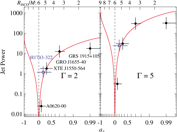
Figure 1.— The relationship between radio jet power, and the observable $R_{\rm ISCO}/M$ (top axis) and black hole spin (bottom axis). The value $a_{*}=0$ is marked by a vertical dashed line. The NM12 data are plotted as filled circles and the data for H1743 as an open square. The uncertainty in jet power is uniformly assumed to be a factor of two.

3.2. Significance of the Result

To evaluate the significance of our fitting results (now including H1743), we have performed a test in which we scrambled the list of observed fluxes – with duplicates allowed – and analyzed these simulated data sets in the same way that we analyzed the actual data. We repeated this randomization process 2500 times for each of our two fiducial values of the Lorentz factor, and in each case a best fit was obtained.

In less than 1% of these trials (6/2500 for $\Gamma=2$, 24/2500 for $\Gamma=5$) is the fit to the randomized data set as good as the fit to the actual data. We conclude that although our sample consists of only five calibration sources, our empirical correlation is nevertheless statistically robust.

4. Predicting the Spins of Black Holes Using the NM12 Model

We now consider six black holes whose spins have not yet been measured via the continuum-fitting method. These systems all displayed a major X-ray outburst during which the source transitioned through the thermal dominant (high-soft) state and produced associated radio flares, which signal the production of jets. Using data in the literature, we estimate the jet power of these black holes and thereby infer their spins by applying the NM12 model. The names of their host transient systems, along with estimates of their peak radio fluxes and distances, are listed in the first three columns of Table 4. Lower limits on the peak X-ray luminosities achieved by these systems are given in Table A.2.

In order to estimate jet power, we require estimates of $M$ and the jet inclination angle $i$, which is problematic for all six systems listed in Table 4. XTE J1720-318 and XTE J1748-288 even lack optical counterparts, while the secondary in GX 339–4 has only been detected via fluoresced emission lines (Hynes et al., 2003). There do exist literature estimates of $M$ and the orbital inclination angle (a proxy for $i$) for the remaining four systems. However, we choose not to use these estimates of $M$ and $i$ because, in our judgment, the light-curve and spectroscopic data that are currently available for these four systems are inadequate to reliably correct the ellipsoidal light curves for the effects of the strong, variable and poorly-determined component of disk light (e.g., see Hynes 2005). We note that this problem has been largely overcome for two similar systems, A0620–00 (Cantrell et al., 2010) and XTE J1550–564 (Orosz et al., 2011), by amassing and analyzing sufficient data, while it is not a significant problem for other systems such as GRO J1655–40 (Greene et al., 2001) and 4U 1543–47 (Orosz et al., 1998) because their much more luminous secondaries strongly outshine their disks. However, for most black hole transients, the systematic uncertainties in $M$ and $i$ still remain sizable (Hynes et al., 2005; Kreidberg et al., 2012).

For all six systems listed in Table 4, we adopt the following approach in assembling the estimates of $M$ and $i$, which we require in order to estimate jet power. First, because no firm mass estimates are available, we use a parametric model for the mass distribution of black holes in transient systems (Equations A1 & A2 in Özel et al. 2012).

Secondly, we make central use of an eminently reliable observable, the mass function,

$$f(M)=\frac{M{\rm sin}^{3}~{}i}{(1+M_{2}/M)^{2}},$$ (6)

where $M_{2}$ is the mass of the companion star. Our results are quite insensitive to the value of $M_{2}$ because $M_{2}/M\ll 1$. In outline, for the four out of six systems in Table 4 with measured values of the mass function, we use $f(M)$ and the black hole mass distribution to compute paired values of $M$ and $i$. We make the standard assumption that the black hole’s spin axis is aligned perpendicular to the binary orbital plane (see Section 5). Then, for given values of $\Gamma$ and $D$ we compute $P_{\rm jet}$. Finally, we use the NM12 model to infer the spins of the black holes.

The spin prediction is computed for each black hole using a Monte Carlo approach as follows. For 1000 iterations, we consider, with uniform weighting, a range of jet speeds from $\Gamma=2$ to $\Gamma=5$, and we randomly vary $f(M)$, $D$, and $S_{\nu}$ according to their measurement errors. A random value of $M$ is drawn from the Özel et al. (2012) distribution, while $M_{2}$ is assigned a random value in the range 0.1–1 $\rm M_{\sun}$. These six parameters are used to calculate $i$ and $P_{\rm jet}$. The data for the five sources of the NM12 model are then refitted using the selected value of $\Gamma$, and finally the value of $a_{*}$ corresponding to $P_{\rm jet}$ is read off the fitted correlation. Table 4 reports the 1$\sigma$ spin ranges for each source, which are based on the assembled Monte-Carlo results.

Table 1Monte-Carlo Spin Predictions

Object	$S_{\nu}^{\rm tot}$(5 GHz) [Jy]	$D$ (kpc)	$f(M)$ ($\rm M_{\sun}$)	Inclination($\arcdeg$)	$a_{*}$	References
GRS 1124–683	0.2–1	$5.9\pm 1.0$	$3.17\pm 0.15$	44–57	0.1–0.4	1, 2–7, but see 8
GX 339–4	0.055	$8\pm 2$	$5.8\pm 0.5$	54–77	0.1–0.4	9–11
		15	$5.8\pm 0.5$	54–77	0.2–0.6	11, 12
XTE J1720–318	0.0047	$6.5\pm 3.5$	$\cdots$	$\cdots$	$<0.1$	13, 14
XTE J1748–288	0.5	$8$	$\cdots$	$\cdots$	0–0.7	15–17
XTE J1859+226	0.10	$8\pm 3$	$4.5\pm 0.6$	50–70	0.1–0.4	4, 18, 19
		14	$4.5\pm 0.6$	50–70	0.2–0.6	19
GS 2000+251	0.005–0.03	$2.7\pm 0.7$	$4.97\pm 0.10$	52–74	$<0.1$	1, 6, 20, 21, 22

References. — (1) Jonker & Nelemans 2004; (2) Ball et al. 1995; (3) Gelino 2001; (4) Hynes 2005; (5) Esin et al. 1997; (6) Barret et al. 1996; (7) Orosz et al. 1996; (8) Shahbaz et al. 1997; (9) Gallo et al. 2004; (10) Zdziarski et al. 2004; (11) Hynes et al. 2003; (12) Hynes et al. 2004; (13) Brocksopp et al. 2005; (14) Chaty & Bessolaz 2006; (15) Brocksopp et al. 2007; (16) Mirabel & Rodríguez 1999; (17) Hjellming et al. 1998; (18) Brocksopp et al. 2002; (19) Corral-Santana et al. 2011; (20) Hjellming et al. 1988; (21) Filippenko et al. 1995; (22) Callanan et al. 1996.

Our results are illustrated in Figure 2. Spin estimates for each black hole are shown in the individual panels, which correspond to our two bracketing values of $\Gamma$ (top and bottom rows) and to three values of $M$ (increasing from left to right), namely the median and 1$\sigma$ limits of the Özel et al. 2012 distribution. Every panel shows a pair of spin values for each of the black holes that have two distance estimates (Table 4).

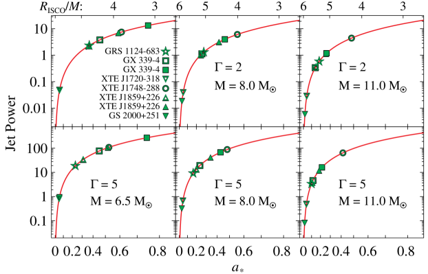
Figure 2.— In successive panels, we plot the spin for each black hole listed in Table 4 that results from adopting a value of $M$ (6.5 $\rm M_{\sun}$, 8$\rm M_{\sun}$, and 11$\rm M_{\sun}$, from left to right) and a value of $\Gamma$ (2 in the upper row and 5 in the lower). The red line in each panel is a fit to the NM12 model using the data for all five calibration sources (Section 3). In producing this figure, we fixed $M_{2}=0.3~{}\rm M_{\sun}$ for the four systems with measured values of the mass function, and arbitrarily show results using $i=60\arcdeg$ for the two without.

5. Comparison with Fe-line Measurements

The relationship between black hole spin and radio jet power (both here and in NM12) has to this point been explored using spin data obtained exclusively by applying the continuum-fitting method. We now investigate pertinent black hole spin data obtained using the Fe-line method. Here, black hole spin is inferred from the breadth and shape of spectral fluorescence features, which are produced in the strong-gravity environment of the inner accretion disk (e.g., Fabian et al. 1989).

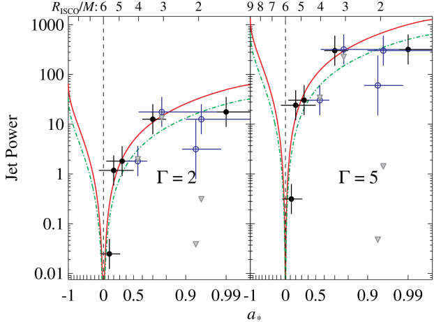
Figure 3.— Fe-line spin measurements (open symbols) are compared against the best-fitting NM12 model – the solid curve – which is based on continuum-fitting spin measurements and a fit to the five calibrations sources (filled circles) shown both here and in Figure 1. A dot-dashed curve shows the best fit achieved to the Fe-line and continuum-fitting measurements together. Both sets of fits have been computed by assuming that all jets are produced with either $\Gamma=2$ (left panel) or $\Gamma=5$ (right panel). The jet powers obtained using the fitted inclinations returned by the Fe-line fits are plotted as filled gray triangles.

Among the black holes that we have so far considered, four have Fe-line spin estimates: GRS 1915+105 ($a_{*}=0.6-1$; Blum et al. 2009), GRO J1655–40 ($a_{*}>0.9$; Reis et al. 2009), GX 339–4 ($a_{*}\approx 0.93$; Miller et al. 2008; Reis et al. 2008), and XTE J1550–564 ($a_{*}\approx 0.55^{+0.10}_{-0.15}$; Steiner et al. 2011). The reported errors for GX 339–4 and GRS  1915+105 are statistical and small (0.01–0.02); in these cases, we adopt $\Delta a_{*}=0.05$ as a rough estimate of the systematic uncertainty.

In considering the Fe-line spin data for these four sources, there are two natural choices for the inclination of the black hole spin vector: the axis perpendicular to the binary orbital plane, or the disk inclination returned from the Fe-line spectral fits. Throughout this paper, we have adhered to the former by assuming that the black hole’s spin is aligned with the orbital angular momentum vector. This assumption is motivated and reasonable because the timescale for alignment (e.g., Martin et al. 2008) is an order of magnitude smaller than the binary lifetime, so that nearly all of the several dozen black holes in known transient systems should presently be well aligned (e.g., see Steiner & McClintock 2012, and references therein).

For the four sources in question, the Fe-line spectral fits return the following estimates of disk inclination (which are determined largely by the blue wing of the fluorescent line features): GRS 1915+105 ($i=55\arcdeg-70\arcdeg$), GRO J1655–40 ($i=30\arcdeg^{+5}_{-10}$), GX 339–4 ($i=20\arcdeg\pm 1\arcdeg$), XTE J1550–564 ($i=71\arcdeg-82\arcdeg$). We caution that these inclination estimates are subject to a systematic uncertainty of order $\sim 10\arcdeg$ for three reasons: The spectral models employed in these fits (1) have not yet accounted for radial variation of ionization across the face of the disk, which can modify the structure of the blue wing of the line profile; (2) omit treatment of Fe $K\beta$ and other (high-order) line transitions that are most important at low or moderate ionization and which can contribute flux just blueward of the dominant Fe $K\alpha$ feature (more recent Fe-line models have now incorporated many additional lines, e.g., García & Kallman 2010); and (3) provide only a cursory treatment of the “warm absorber” features introduced by ionized disk winds. Warm absorbers, in the notable case of GRO J1655–40, have been found to vary with state and to contribute dozens of spectral lines at high significance (Miller et al., 2006; Neilsen & Homan, 2012).

Although these three effects degrade estimates of inclination, which depend on the extent of the blue wing of the line, they have a minor affect on the spin parameter because it is determined principally by the red wing of the line, which is an order of magnitude broader than the energy shift induced in the blue wing by varying inclination (see e.g., Reis et al. 2009, 2012; Fabian et al. 2012). Therefore, with a reasonable degree of confidence, we make use of the fitted spins while at the same time adopting the assumption of alignment, and so we choose the orbital inclination angle over the inclination angle returned by the Fe-line fits.

In Figure 3, the Fe-line results are shown alongside the data for our five calibration sources from Figure 1. Because none of the Fe-line sources has a low spin, the Fe-line data alone only weakly test the NM12 model. At the same time, the Fe-line and continuum-fitting results are reasonably consistent. The dash-dotted curve shows a best fit based on both the continuum-fitting and Fe-line spin data. The normalization for this fit is roughly a factor of two lower than results from continuum-fitting alone (primarily because of the relatively high Fe-line spin and low radio flux from GX 339–4). This shift is very small compared to the three orders of magnitude spanned in jet power.

We note that our conclusion that the Fe-line spin measurements are consistent with the NM12 model is contingent upon the use of orbital inclinations. That is, results obtained using the inclinations returned by the Fe-line fits (shown by the solid triangle symbols in Figure 3) are inconsistent with the NM12 model. This is due to the large difference in the beaming correction implied by the Fe-line inclinations for GX 339–4 and GRO J1655–40.

6. Discussion

An inspection of Figure 2 reveals that the inferred jet power increases with $\Gamma$ because the inclination angles are generally high ($i\gtrsim 35\arcdeg$; see Section 2 and Table 4) for the sample of six black holes in Table 4. We now consider the effect of increasing the mass (for a fixed value of the mass function): This decreases $i$ and increases the Doppler factor, thereby decreasing the inferred jet power and the spin. Thus, with the radio flux fixed at its observed value, a high value of $M$ implies low spin. In particular, for $M\gtrsim 8\rm M_{\sun}$, none of the black holes of Table 4 is expected to have a spin above $a_{*}\approx 0.5$.

Therefore, based on the NM12 model, the sample of six black holes in Table 4 is expected to have low masses, low spins, or both. An additional outcome of the model is that, as an ensemble, the transient black holes contrast starkly with the three wind-fed, X-ray-persistent black holes, which have masses in the range $M=11-16~{}\rm M_{\sun}$ and spins ranging from $a_{*}=0.85$ to $a_{*}>0.95$ (Gou et al. 2011, and references therein). This suggests a dichotomy between the black holes that form in these two distinct classes of binary systems.

Table 4 shows that each of the predicted black hole spin values is expected to be below $a_{*}=0.7$. Furthermore, two sources, XTE J1720–318 and GS 2000+25, may have record low values of spin. Measuring their spins directly will provide a strong test of the NM12 model. We note that our result for GX 339–4, $a_{*}<0.6$, is consistent with the upper limit from continuum-fitting by Kolehmainen & Done (2010).

In addition to predicting the spins of six black holes, we have also provided estimates of the orbital inclination angles of their host binaries by using the semiempirical mass distribution of Özel et al. (2012). Future ground-based and X-ray studies will sharpen up the estimates of $M$, $i$ and $D$ that we have used here and can lead to direct measurements of spin, thereby testing the predictions laid out in Table 4.

7. Conclusions

Under the assumption that the 5 GHz peak radio flux density from transient black holes can be used as a proxy for their jet power, the work of Narayan & McClintock (2012) demonstrates a clear and empirical link between jet power and black hole spin, as predicted by Blandford & Znajek (1977). The addition of a fifth calibration source, H1743–322, whose spin and jet power are entirely consistent with the NM12 model, strengthens that link. For a moderate and appropriate range of jet speeds ($\Gamma=2-5$), we have used the jet-power vs. spin correlation for all five calibration sources to predict the spins of six black hole primaries located in transient systems, which contain low-mass secondaries. Surprisingly, all of these predicted spins are relatively low, $a_{*}<0.7$, especially when compared to the spins of the black hole primaries in the persistent and wind-fed systems ($a_{*}>0.85$), which have massive companions. Future measurements of spin can be used to test these predictions and the NM12 model.

Appendix A A Basis for the Standard Candle Assumption

In Section 1, we assert that at X-ray maximum a black hole transient approaches its Eddington limit and that it therefore reasonably approximates a standard candle. This is a crucial assumption because it implies that the accretion power ($\dot{M}/M$) is roughly the same in different objects when they exhibit ballistic jets. This allows us to meaningfully compare the jet powers (i.e., the peak mass-scaled radio luminosities) of the various sources in our sample, which vary by a factor of 700 for a uniform assumed value of $\Gamma=2$ and by a factor of 1000 for $\Gamma=5$ (Fig. 1).

It is problematic to test this standard candle assumption for several reasons. The most important of these is that in nearly all observations of black hole transients much of the X-ray flux falls outside the passband of the detector, and, at the same time, there is no standard model one can use to make a bolometric correction. With this in mind, we compute firm lower limits to the peak luminosities of these sources using model fluxes reported in the literature that fall within the passband of the detector in question. This straightforward and empirical approach necessarily yields underestimates of peak luminosity because it ignores flux at the high- and low-energy ends of the spectrum.

In our discussion, we consider only black hole transients that have made a hard-to-soft transition. In particular, we disregard the several systems discussed by Brocksopp et al. (2004) that have never made this transition, and we also disregard “failed” outbursts of other systems that stalled in the low/hard state (e.g., the 2001 and 2002 outbursts of XTE J1550–564; see Fig. 6$a$ in Remillard & McClintock 2006). In Section A.1 below, we consider only the largest outburst that has been observed for each of the sources in our sample. We show that each of our five calibration sources, which have relatively high quality distance estimates, reaches about half or more of its Eddington limit during a major outburst. In Section A.2, we further show that even if the distance is poorly known one can conclude that the peak luminosity of a black hole transient is at least $\approx 10$% of Eddington if the source has made a hard-to-soft transition.

A.1. Peak Luminosities during Major Outbursts

Our determinations of the peak observed component of the Eddington-scaled luminosities of ten sources are given in the two rightmost data columns in Table A.2: $L_{\rm Peak}/L_{\rm Edd}$ is the isotropic (Eddington-scaled) luminosity and $L_{\rm Disk,Peak}/L_{\rm Edd}$ is the luminosity assuming that the emitter is a thin disk (see Table footnote $b$ in Table A.2). In the former case, the mean observed component of luminosity for the the five calibration sources in the top half of the table is $0.57\pm 0.25$ (std. dev.), and in the latter case it is $0.76\pm 0.30$ (where we have assumed that GRS 1915+105 is at its Eddington limit). Thus, we conclude that our calibration sources typically reach half or more of their Eddington limit during a major outburst.

We note that our conclusion is corroborated by an independent analysis for a sample of black hole transients considered by Dunn et al. (2010). Their results for the peak luminosities of these sources, all of which have undergone a hard-to-soft transition, are summarized in their Figure 11. For the four recurrent sources (XTE J1550–564, 4U 1630–47, GX 339–4 and H1743–322), we restrict our attention to the brightest outburst for each source. For H1743 only, we correct the luminosity given by Dunn et al. using $D=8.5$ kpc (Steiner et al., 2012) in place of their guess of 5 kpc. We disregard SLX 1746-331 whose distance is essentially unconstrained within the Galaxy. The mean isotropic luminosity of the remaining sample of eight sources is $L_{\rm Peak}/L_{\rm Edd}=0.43\pm 0.23$ (std. dev.), which is quite comparable to our result quoted above. Dunn et al. obtain a somewhat lower value than we do because they consider only the 2–10 keV component of luminosity while we generally consider wider bandpasses (see below).

We now present the details of our analysis that support the italicized conclusion stated above. The sources listed in the top half of Table A.2 are our calibration sources (Fig. 1), and those in the lower half are the sources listed in Table 4. (We disregard XTE J1720–318 because there are no suitable X-ray data near maximum). The distance and mass estimates are taken from Table 1 in NM12 and Table 4 herein, except for the six black holes that lack mass measurements; for these we adopt the nominal value $M=8~{}M_{\odot}$ (Özel et al., 2010; Farr et al., 2011). As discussed below, for all but two sources, GRO J1655–40 and GRS 1915+105, the tabulated value of $L_{\rm Peak}/L_{Edd}$ at X-ray maximum was computed for the corresponding radio outburst used in estimating the jet power. In all cases, our peak luminosities are based on the peak unabsorbed fluxes that have been reported in the literature for the missions and bandpasses listed in Table A.2.

The firm lower limits on peak luminosities given in Table A.2 are strictly empirical; i.e., they are computed directly from the observed maximum fluxes $F_{\rm max}$ assuming either an isotropic source, $L_{\rm Peak}/L_{Edd}={{4\pi}{D^{2}}{F_{\rm max}}}/({{1.3}{\times}{10^{38}}{M/M_{\odot}}}$), or alternatively a thin disk (see footnote $b$ in Table A.2).

A0620–00: Doxsey et al. (1976) report a 1–10 keV flux at the maximum of the 1975 outburst of $F_{\rm max}(1-10~{}$keV$)=1.7\times 10^{-6}$ for a thermal bremsstrahlung spectrum with $kT=1.7$ keV. Sixteen days later, they made a second observation, this time additionally employing the SAS–3 low-energy system (0.15–0.9 keV). The spectral parameters and flux derived for this latter observation allow one to conclude that the 0.3–1 keV flux was 2.04 times the 1–10 keV flux. Taking this result as a guide and using the spectrum determined by Doxsey et al. at maximum, we find that the 0.3–1 keV flux at that time was 1.77 times the 1–10 keV flux. We therefore conclude: $F_{\rm max}(0.3-10~{}$keV$)=3.0\times 10^{-6}$ ergs cm^-2 s^-1..

XTE J1550–564: Here we use the X-ray flux reported at the peak of the extraordinary 7-Crab flare, which was observed on 1998 September 19, and which preceded the detection of the radio ejection by four days (Hannikainen et al., 2009). We adopt the 2–20 keV and 20–100 keV fluxes reported by Sobczak et al. (2000) respectively in their Tables 3 & 4: $F_{\rm max}(2-100~{}$keV$)=2.72\times 10^{-7}$ ergs cm^-2 s^-1.

GRO J1655–40: Major X-ray outbursts of this source were observed in 1994, 1996 and 2005. Unfortunately, radio data at X-ray maximum were obtained only for the 1994 outburst (see Table 1 in NM12), and the available X-ray data at maximum for this outburst (BATSE at $E>20$ keV) do not provide a useful lower limit on $L_{\rm Peak}/L_{Edd}$. Therefore, in estimating $L_{\rm Peak}/L_{Edd}$ for this source, we consider the well-observed 1996 and 2005 outbursts, which had very comparable peak intensities of $\approx 300~{}{\it RXTE}$ ASM counts s^-1, 2–12 keV (Sobczak et al., 1999; Brocksopp et al., 2006). As our proxy for the 1994 X-ray peak flux, we adopt the peak flux observed for the 2005 outburst on May 16 by Brocksopp et al. because the Swift XRT and BAT detectors provide broadband coverage with superior low-energy coverage; we find: $F_{\rm max}(0.7-150~{}$keV$)=2.26\times 10^{-7}$ ergs cm^-2 s^-1.

H1743–322: As in the case of XTE J1550–564, and as discussed in Section 3, the jet was launched by an impulsive power-law flare, which was observed on 2003 May 6 (MJD 52765.9); the radio flux reached a maximum $\approx 2.6$ days later (McClintock et al., 2009). The peak X-ray flux reported in Table A2 of McClintock et al. is $F_{\rm max}(2-100~{}$keV$)=5.84\times 10^{-8}$ ergs cm^-2 s^-1.

GS 1915+105: As in the case of GRO 1655–40, poor X-ray coverage does not allow us to set a useful lower limit on $L_{\rm Peak}/L_{Edd}$ for either of the well-studied radio outbursts considered in NM12 (Rodriguez et al., 1995; Fender et al., 1999). Furthermore, the distance to this source is quite uncertain, ranging from about 7 kpc to above 12 kpc (see Fig. 18 in McClintock et al. 2006). We therefore fall back on the widely accepted conclusion that this source is generally exceptionally luminous. For example, Done et al. (2004) infer luminosities as high as $\approx 1.7$ Eddington for $D=12.5$ kpc (or 1.0 Eddington for 9.5 kpc). We therefore assume, as indicated in Table A.2, that the source was near its Eddington limit at the time of peak radio emission on 1994 March 24 (Rodriguez et al., 1995).

GRS 1124–683 (Nova Mus 1991): In their Table 2, Ebisawa et al. (1994) summarize the spectral parameters and fluxes for frequent observations of this source during its 1991 outburst. For the peak-flux observation of 1991 January 16 at 19 hours UT, we adopt their tabulated value of the hard flux in the 2–20 keV band and, using the spectral parameters given for the thermal component, compute the corresponding soft flux in this same band and conclude: $F_{\rm max}(2-20~{}$keV$)=1.53\times 10^{-7}$ ergs cm^-2 s^-1.

GX 339–4: The times of the peak radio flux (Gallo et al., 2004) and the peak RXTE ASM count rate coincided within roughly one day. We adopt the peak X-ray flux plotted in Figure 9 (panel b) in Remillard & McClintock (2006): $F_{\rm max}(2-20~{}$keV$)=2.20\times 10^{-8}$ ergs cm^-2 s^-1.

XTE J1748–288: Both the X-ray and radio coverage are relatively spotty for this source (Brocksopp et al., 2007). In estimating the peak X-ray flux, we use the results of the analysis of an RXTE PCA spectrum that was obtained at the time of peak intensity as recorded by the RXTE ASM. This spectrum is plotted in Figure 4.14 and the spectral parameters are tabulated in Table 4.4 in McClintock & Remillard (2006). Using these data, we find: $F_{\rm max}(2-20~{}$keV$)=3.06\times 10^{-8}$ ergs cm^-2 s^-1.

XTE J1859+226: As in the case of GX 339–4, the radio flux and the RXTE ASM count rate peaked within about a day of each other. We adopt the peak X-ray flux plotted in Figure 8 (panel b) in Remillard & McClintock (2006): $F_{\rm max}(2-20~{}$keV$)=3.55\times 10^{-8}$ ergs cm^-2 s^-1.

GS 2000+25: The peak of the outburst occurred on 1988 April 28 (Tsunemi et al., 1989). As a lower bound, we adopt the flux for an observation made two days after the peak, on April 30, which is reported by Terada et al. (2002) in their Tables 2–5: $F_{\rm max}(1.7-37~{}$keV$)=2.6\times 10^{-7}$ ergs cm^-2 s^-1.

XTE J1720–318: While we give a spin estimate for this source (Table 4), we exclude it in Table A.2 because (apart from the RXTE ASM) there is no information on its spectrum at maximum. If we make the arbitrary assumption that its spectrum and flux is the same as that of XTE J1748–288 (see above), then adopting $M=8~{}M_{\odot}$ and the very uncertain distance estimate of $D=6.5$ kpc, we find $L_{\rm Peak}/L_{\rm Edd}=0.15$. (We note that for this source, even at twice the nominal distance, the spin prediction remains very low, $a_{*}\lesssim 0.14$.)

A.2. A Floor on the Peak Luminosity

Finally, we present evidence for a floor on the peak luminosity of systems that undergo a hard to soft transition through the thermal state. As mentioned at the outset of Section 4, such a state transition is one of our selection criteria. Setting a minimum peak luminosity is important for sources whose distances are relatively uncertain, such as most of the sources listed in Table 1. We again use the luminosity data summarized by Dunn et al. (2010) in their Figure 11 (and we again exclude SLX 1746–331 and adopt $D=8.5$ kpc for H1743–32).

For each of the four recurrent sources, Dunn et al. plot the peak luminosities for between two and four separate outburst cycles. Considering now the faintest outburst for each of the four recurrent sources, we conclude that the peak luminosity of all eight sources in the Dunn et al. sample exceeds 8% of Eddington, which is to be compared to the factor of $\sim 1000$ range in the peak radio luminosities of our five calibration sources. Again, this floor of 8% of Eddington is a very conservative lower limit because Dunn et al. consider only the 2–10 keV component of luminosity.

Table A1Observed Component of Luminosity at Outburst Maximum

Object	$D$(kpc)	$M(M_{\odot}$)	Mission	Band (keV)	$L_{\rm Peak}/L_{\rm Edd}$	$L_{\rm Disk,Peak}/L_{\rm Edd}$	References
A0620-00	1.06	6.6	SAS-3	0.3–10	0.47	0.37	1
XTE J1550–564	4.38	9.1	RXTE	2–100	0.53	1.00	2
GRO J1655–40	3.2	6.3	Swift	0.7-150	0.34	0.50	3
H1743–322	8.5	8	RXTE	2–100	0.49	0.94	4
GRS 1915+105	11	14	RXTE	2–20	$\sim 1$	$\sim 1$	5,6
GRS 1124–683	5.9	8	Ginga	2–20	0.61	0.48	7
GX 339–4	8	8	RXTE	2–20	0.16	0.20	8
	15				0.57	0.69
XTE J1748–288	8	8	RXTE	2–20	0.23	0.16	6
XTE J1859+226	8	8	RXTE	2–20	0.26	0.26	8
	14				0.80	0.80
GS2000+25	2.7	8	Ginga	1.7–37	0.22	0.24	9

.

References. — (1) Doxsey et al. 1976; (2) Sobczak et al. 2000; (3) Brocksopp et al. 2006; (4) McClintock et al. 2009; (5) Done et al. 2004; (6) McClintock & Remillard 2006; (7) Ebisawa et al. 1994; (8) Remillard & McClintock 2006; (9) Terada et al. 2002.

Appendix B Estimating the Energy of Ballistic Synchrotron Bubbles

In the toy analysis that follows, we derive a relationship between synchrotron emission from a plasmoid and its bulk kinetic energy. This derivation is not intended to be rigorous. Rather, our aim is to demonstrate that a roughly linear relationship between synchrotron flux density at light-curve maximum and blob kinetic energy – as assumed by the empirical NM12 model – is a natural outcome of classical jet theory. We stress that this derivation is applicable to impulsive, ballistic jets (e.g., Mirabel & Rodríguez 1994; Hjellming & Rupen 1995) as opposed to steady-state jets, which are described by a different class of models (e.g., Heinz & Sunyaev 2003; Fender 2001; Falcke & Biermann 1996). For additional background on the synchrotron-bubble model discussed here, we refer the interested reader to van der Laan (1966); Kellermann & Owen (1988); Hjellming et al. (1988); Hjellming & Johnston (1988).

We assume that all beaming-related effects ($\Gamma$ dependence) have been removed. That is, we work in the frame of a single radiating blob. We are interested in the relation between the radio luminosity of the blob at 5 GHz and the energy of the blob. Using a fairly standard set of assumptions for synchrotron-emitting blobs (e.g., Hjellming & Johnston 1988), we derive such a relationship. The following calculation is approximate and ignores certain factors of order unity, but it is dimensionally correct.

Let $B$ be the magnetic field strength, and let $\gamma$ be the typical Lorentz factor of the electrons that produce synchrotron radiation at 5 GHz. From standard synchrotron theory,

$$\nu_{\rm synch}=\frac{3}{4\pi}\,\gamma^{2}\,\frac{eB}{m_{e}c}=5\,{\rm GHz},$$ (B1)

which gives

$$B=1200\,\gamma^{-2}~{}{\rm G}.$$ (B2)

Let us assume that the electrons in the blob have an energy distribution of the form

$$N(\gamma)\,d\gamma=N_{0}\,\gamma^{-p}\,d\gamma,\quad\gamma\geq 1,$$ (B3)

where for simplicity we assume that the minimum energy of the electrons is $\gamma_{\rm min}\approx 1$. The effective number of electrons radiating at 5 GHz is then

$$N_{\gamma}\approx\gamma\,N(\gamma)=N_{0}\,\gamma^{-(p-1)}.$$ (B4)

The synchrotron luminosity of these electrons is

$$\nu L_{\nu}\approx N_{\gamma}\,\frac{2e^{4}}{3m_{e}^{2}c^{3}}\,\gamma^{2}B^{2}\,\frac{1}{2}=1.1\times 10^{-9}\,N_{\gamma}\gamma^{-2}~{}{\rm erg\,s^{-1}},$$ (B5)

where the factor of $1/2$ in the middle expression is to allow for the fact that $d\ln\nu=2\,d\ln\gamma$ (eq. B1).

Let us assume that there is rough equipartition between the energy in the magnetic field and that in the relativistic electrons. Assuming that the radius of the blob is $R$, we write the equipartition condition as

$$\frac{B^{2}}{8\pi}\,\frac{4\pi}{3}R^{3}=\xi\,N_{0}\,m_{e}c^{2},$$ (B6)

where the dimensionless number $\xi$ measures the deviation from strict equipartition.

We now make use of the fact that, at the peak of the radio light-curve, the synchrotron radiation makes a transition from self-absorbed radiation to optically thin emission. Writing the effective temperature $T_{\gamma}$ of the relevant electrons as

$$kT_{\gamma}=\gamma m_{e}c^{2},$$ (B7)

the condition of marginal self-absorption requires the radio luminosity at the light-curve maximum to satisfy

$$\left(\nu L_{\nu}\right)_{\rm max}=1.1\times 10^{-9}\,N_{\gamma}\gamma^{-2}~{}{\rm erg\,s^{-1}}=4\pi R^{2}\,\pi\nu\,2\,\frac{\nu^{2}}{c^{2}}\,kT_{\gamma}.$$ (B8)

We have used the Rayleigh-Jeans approximation for the expression on the right.

For ease of comparison with our previous work and with the discussion in the main text, we express the luminosity $(\nu L_{\nu})_{\rm max}$ in terms of the quantity $P_{\rm jet}$ (see eq. 3):

$$P_{\rm jet}\equiv\frac{(\nu S_{\nu})_{\rm max}D^{2}}{M}~{}{\rm kpc^{2}\,GHz\,Jy\,M_{\odot}^{-1}},$$ (B9)

which is defined in practical units. In what follows, we assume for simplicity that $M=10M_{\odot}$. Hence

$$\left(\nu L_{\nu}\right)_{\rm max}=4\pi\,\left(\nu S_{\nu}\right)_{\rm max}\,D^{2}=1.2\times 10^{31}P_{\rm jet}~{}{\rm erg\,s^{-1}}.$$ (B10)

We have collected enough relations to solve for all quantities in terms of the single observable quantity $P_{\rm jet}$. Let us assume that $p=5/2$, which corresponds to an optically thin synchrotron spectrum $S_{\nu}\propto\nu^{-0.75}$. For this reasonable value of $p$, we obtain

$$B \approx 2.4\,\xi^{2/9}P_{\rm jet}^{-1/9}~{}{\rm G},$$ (B11)

$$\gamma \approx 22\,\xi^{-1/9}P_{\rm jet}^{1/18},$$ (B12)

$$N_{0} \approx 5.5\times 10^{44}\,\xi^{-7/18}P_{\rm jet}^{43/36},$$ (B13)

$$R \approx 7.7\times 10^{12}\,\xi^{1/18}P_{\rm jet}^{17/36}~{}{\rm cm}.$$ (B14)

In obtaining these results, we have assumed that $P_{\rm jet}$ is measured from the peak radio luminosity at 5 GHz (in fact, all our relations assume $\nu=5$ GHz). Interestingly, the equipartition factor $\xi$ turns out to be relatively unimportant.

The above results allow us to estimate various quantities in the frame of the blob. To calculate the relativistic bulk kinetic energy of the blob in the “lab” frame, we assume that there is one proton for each electron, i.e., a total of $\approx N_{0}$ protons in the blob. Since the thermal energy in the electrons is small compared to the rest mass energy of the protons, we expect the protons to be effectively cold. Let the blob move with bulk Lorentz factor $\Gamma$ in the lab frame. In this frame, the blob energy is dominated by the proton kinetic energy. Hence, we estimate the energy in the blob to be

$$E_{\rm blob}\approx N_{0}\,\Gamma m_{p}c^{2}\approx 8.3\times 10^{41}\,\Gamma\,\xi^{-7/18}P_{\rm jet}^{43/36}~{}{\rm erg}.$$ (B15)

The numerical values we have obtained above should not be taken too seriously considering the approximations we have made. However, they are reasonable. For instance, for the microquasar GRS 1915+105, if we take $P_{\rm jet}\sim 100$, we estimate the rest mass of the blob to be $N_{0}m_{p}\approx 2\times 10^{23}\,{\rm g}$, and for $\Gamma\sim 5$ we find the bulk kinetic energy to be $\sim 10^{45}\,{\rm erg}$. These estimates are fairly close to those obtained by Rodríguez & Mirabel (1999) even though they followed a different approach, using the angular size of the blob instead of the light-curve maximum.

For our present purposes, the key result from the above analysis is the scaling in equation (B15), which shows that the bulk kinetic energy of the blob is expected to vary approximately as the 1.2 power of the 5 GHz radio power ($P_{\rm jet}$) at light-curve maximum, i.e., there is a more or less linear relation between the two quantities. This provides strong support for our reliance upon $P_{\rm jet}$ as a measure of the jet kinetic power.

References

- Ball et al. (1995) Ball, L., Kesteven, M. J., Campbell-Wilson, D., Turtle, A. J., & Hjellming, R. M. 1995, MNRAS, 273, 722
- Bardeen et al. (1972) Bardeen, J. M., Press, W. H., & Teukolsky, S. A. 1972, ApJ, 178, 347
- Barret et al. (1996) Barret, D., McClintock, J. E., & Grindlay, J. E. 1996, ApJ, 473, 963
- Beckwith et al. (2008) Beckwith, K., Hawley, J. F., & Krolik, J. H. 2008, ApJ, 678, 1180
- Blandford & Znajek (1977) Blandford, R. D., & Znajek, R. L. 1977, MNRAS, 179, 433
- Blum et al. (2009) Blum, J. L., Miller, J. M., Fabian, A. C., Miller, M. C., Homan, J., van der Klis, M., Cackett, E. M., & Reis, R. C. 2009, ApJ, 706, 60
- Brocksopp et al. (2004) Brocksopp, C., Bandyopadhyay, R. M., & Fender, R. P. 2004, NewA, 9, 249
- Brocksopp et al. (2005) Brocksopp, C., Corbel, S., Fender, R. P., Rupen, M., Sault, R., Tingay, S. J., Hannikainen, D., & O’Brien, K. 2005, MNRAS, 356, 125
- Brocksopp et al. (2002) Brocksopp, C., et al. 2002, MNRAS, 331, 765
- Brocksopp et al. (2006) —. 2006, MNRAS, 365, 1203
- Brocksopp et al. (2007) Brocksopp, C., Miller-Jones, J. C. A., Fender, R. P., & Stappers, B. W. 2007, MNRAS, 378, 1111
- Callanan et al. (1996) Callanan, P. J., Garcia, M. R., Filippenko, A. V., McLean, I., & Teplitz, H. 1996, ApJ, 470, L57
- Cantrell et al. (2010) Cantrell, A. G., et al. 2010, ApJ, 710, 1127
- Chaty & Bessolaz (2006) Chaty, S., & Bessolaz, N. 2006, A&A, 455, 639
- Corbel et al. (2005) Corbel, S., Kaaret, P., Fender, R. P., Tzioumis, A. K., Tomsick, J. A., & Orosz, J. A. 2005, ApJ, 632, 504
- Corbel et al. (2007) Corbel, S., Tzioumis, T., Brocksopp, C., & Fender, R. 2007, The Astronomer’s Telegram, 1007, 1
- Corral-Santana et al. (2011) Corral-Santana, J. M., Casares, J., Shahbaz, T., Zurita, C., Martínez-Pais, I. G., & Rodríguez-Gil, P. 2011, MNRAS, 413, L15
- Done et al. (2004) Done, C., Wardziński, G., & Gierliński, M. 2004, MNRAS, 349, 393
- Doxsey et al. (1976) Doxsey, R., et al. 1976, ApJ, 203, L9
- Dunn et al. (2010) Dunn, R. J. H., Fender, R. P., Körding, E. G., Belloni, T., & Cabanac, C. 2010, MNRAS, 403, 61
- Ebisawa et al. (1993) Ebisawa, K., Makino, F., Mitsuda, K., Belloni, T., Cowley, A. P., Schmidtke, P. C., & Treves, A. 1993, ApJ, 403, 684
- Ebisawa et al. (1991) Ebisawa, K., Mitsuda, K., & Hanawa, T. 1991, ApJ, 367, 213
- Ebisawa et al. (1994) Ebisawa, K., et al. 1994, PASJ, 46, 375
- Esin et al. (1997) Esin, A. A., McClintock, J. E., & Narayan, R. 1997, ApJ, 489, 865
- Fabian et al. (1989) Fabian, A. C., Rees, M. J., Stella, L., & White, N. E. 1989, MNRAS, 238, 729
- Fabian et al. (2012) Fabian, A. C., et al. 2012, MNRAS, 424, 217
- Falcke & Biermann (1996) Falcke, H., & Biermann, P. L. 1996, A&A, 308, 321
- Farr et al. (2011) Farr, W. M., Sravan, N., Cantrell, A., Kreidberg, L., Bailyn, C. D., Mandel, I., & Kalogera, V. 2011, ApJ, 741, 103
- Fender (2006) Fender, R. 2006, Jets from X-ray binaries (Cambridge, UK, Cambridge University Press), 381–419
- Fender (2001) Fender, R. P. 2001, MNRAS, 322, 31
- Fender et al. (2004) Fender, R. P., Belloni, T. M., & Gallo, E. 2004, MNRAS, 355, 1105
- Fender et al. (2010) Fender, R. P., Gallo, E., & Russell, D. 2010, MNRAS, 1009
- Fender et al. (1999) Fender, R. P., Garrington, S. T., McKay, D. J., Muxlow, T. W. B., Pooley, G. G., Spencer, R. E., Stirling, A. M., & Waltman, E. B. 1999, MNRAS, 304, 865
- Filippenko et al. (1995) Filippenko, A. V., Matheson, T., & Barth, A. J. 1995, ApJ, 455, L139
- Gallo et al. (2004) Gallo, E., Corbel, S., Fender, R. P., Maccarone, T. J., & Tzioumis, A. K. 2004, MNRAS, 347, L52
- García & Kallman (2010) García, J., & Kallman, T. R. 2010, ApJ, 718, 695
- Gelino (2001) Gelino, D. M. 2001, PhD thesis, Center for Astrophysics and Space Sciences, University of California, San Diego
- Gou et al. (2011) Gou, L., et al. 2011, ApJ, 742, 85
- Greene et al. (2001) Greene, J., Bailyn, C. D., & Orosz, J. A. 2001, ApJ, 554, 1290
- Hannikainen et al. (2009) Hannikainen, D. C., et al. 2009, MNRAS, 397, 569
- Heinz & Sunyaev (2003) Heinz, S., & Sunyaev, R. A. 2003, MNRAS, 343, L59
- Hjellming et al. (1988) Hjellming, R. M., Calovini, T. A., Han, X. H., & Cordova, F. A. 1988, ApJ, 335, L75
- Hjellming & Johnston (1988) Hjellming, R. M., & Johnston, K. J. 1988, ApJ, 328, 600
- Hjellming & Rupen (1995) Hjellming, R. M., & Rupen, M. P. 1995, Nature, 375, 464
- Hjellming et al. (1998) Hjellming, R. M., Rupen, M. P., Mioduszewski, A. J., Smith, D. A., Harmon, B. A., Waltman, E. B., Ghigo, F. D., & Pooley, G. G. 1998, in Bulletin of the American Astronomical Society, Vol. 30, American Astronomical Society Meeting Abstracts, 103.08
- Hynes (2005) Hynes, R. I. 2005, ApJ, 623, 1026
- Hynes et al. (2005) Hynes, R. I., Robinson, E. L., & Bitner, M. 2005, ApJ, 630, 405
- Hynes et al. (2003) Hynes, R. I., Steeghs, D., Casares, J., Charles, P. A., & O’Brien, K. 2003, ApJ, 583, L95
- Hynes et al. (2004) —. 2004, ApJ, 609, 317
- Jonker & Nelemans (2004) Jonker, P. G., & Nelemans, G. 2004, MNRAS, 354, 355
- Kellermann & Owen (1988) Kellermann, K. I., & Owen, F. N. 1988, Radio galaxies and quasars (Springer-Verlag, Berlin and New York), 563–602
- Kolehmainen & Done (2010) Kolehmainen, M., & Done, C. 2010, MNRAS, 406, 2206
- Kreidberg et al. (2012) Kreidberg, L., Bailyn, C. D., Farr, W. M., & Kalogera, V. 2012, ApJ, 757, 36
- Livio (1999) Livio, M. 1999, Phys. Rep., 311, 225
- Martin et al. (2008) Martin, R. G., Tout, C. A., & Pringle, J. E. 2008, MNRAS, 387, 188
- McClintock et al. (2011) McClintock, J. E., et al. 2011, Classical and Quantum Gravity, 28, 114009
- McClintock & Remillard (2006) McClintock, J. E., & Remillard, R. A. 2006, Black hole binaries (Cambridge, UK, Cambridge University Press), 157–213
- McClintock et al. (2009) McClintock, J. E., Remillard, R. A., Rupen, M. P., Torres, M. A. P., Steeghs, D., Levine, A. M., & Orosz, J. A. 2009, ApJ, 698, 1398
- McClintock et al. (2006) McClintock, J. E., Shafee, R., Narayan, R., Remillard, R. A., Davis, S. W., & Li, L.-X. 2006, ApJ, 652, 518
- McKinney & Blandford (2009) McKinney, J. C., & Blandford, R. D. 2009, MNRAS, 394, L126
- Miller et al. (2006) Miller, J. M., Raymond, J., Fabian, A., Steeghs, D., Homan, J., Reynolds, C., van der Klis, M., & Wijnands, R. 2006, Nature, 441, 953
- Miller et al. (2008) Miller, J. M., et al. 2008, ApJ, 679, L113
- Miller-Jones et al. (2012) Miller-Jones, J. C. A., et al. 2012, MNRAS, 421, 468
- Mirabel & Rodríguez (1994) Mirabel, I. F., & Rodríguez, L. F. 1994, Nature, 371, 46
- Mirabel & Rodríguez (1999) —. 1999, ARA&A, 37, 409
- Narayan & McClintock (2012) Narayan, R., & McClintock, J. E. 2012, MNRAS, 419, L69
- Neilsen & Homan (2012) Neilsen, J., & Homan, J. 2012, ApJ, 750, 27
- Orosz et al. (1996) Orosz, J. A., Bailyn, C. D., McClintock, J. E., & Remillard, R. A. 1996, ApJ, 468, 380
- Orosz et al. (1998) Orosz, J. A., Jain, R. K., Bailyn, C. D., McClintock, J. E., & Remillard, R. A. 1998, ApJ, 499, 375
- Orosz et al. (2011) Orosz, J. A., Steiner, J. F., McClintock, J. E., Torres, M. A. P., Remillard, R. A., Bailyn, C. D., & Miller, J. M. 2011, ApJ, 730, 75
- Özel et al. (2010) Özel, F., Psaltis, D., Narayan, R., & McClintock, J. E. 2010, ApJ, 725, 1918
- Özel et al. (2012) Özel, F., Psaltis, D., Narayan, R., & Santos Villarreal, A. 2012, ApJ, 757, 55
- Reis et al. (2009) Reis, R. C., Fabian, A. C., Ross, R. R., & Miller, J. M. 2009, MNRAS, 395, 1257
- Reis et al. (2008) Reis, R. C., Fabian, A. C., Ross, R. R., Miniutti, G., Miller, J. M., & Reynolds, C. 2008, MNRAS, 387, 1489
- Reis et al. (2012) Reis, R. C., Miller, J. M., Reynolds, M. T., Fabian, A. C., & Walton, D. J. 2012, ApJ, 751, 34
- Remillard & McClintock (2006) Remillard, R. A., & McClintock, J. E. 2006, ARA&A, 44, 49
- Rodriguez et al. (1995) Rodriguez, L. F., Gerard, E., Mirabel, I. F., Gomez, Y., & Velazquez, A. 1995, ApJS, 101, 173
- Rodríguez & Mirabel (1999) Rodríguez, L. F., & Mirabel, I. F. 1999, ApJ, 511, 398
- Shahbaz et al. (1997) Shahbaz, T., Naylor, T., & Charles, P. A. 1997, MNRAS, 285, 607
- Shrader et al. (1994) Shrader, C. R., Wagner, R. M., Hjellming, R. M., Han, X. H., & Starrfield, S. G. 1994, ApJ, 434, 698
- Sobczak et al. (1999) Sobczak, G. J., McClintock, J. E., Remillard, R. A., Bailyn, C. D., & Orosz, J. A. 1999, ApJ, 520, 776
- Sobczak et al. (2000) Sobczak, G. J., McClintock, J. E., Remillard, R. A., Cui, W., Levine, A. M., Morgan, E. H., Orosz, J. A., & Bailyn, C. D. 2000, ApJ, 544, 993
- Steiner & McClintock (2012) Steiner, J. F., & McClintock, J. E. 2012, ApJ, 745, 136
- Steiner et al. (2012) Steiner, J. F., McClintock, J. E., & Reid, M. J. 2012, ApJ, 745, L7
- Steiner et al. (2011) Steiner, J. F., et al. 2011, MNRAS, 416, 941
- Tchekhovskoy et al. (2010) Tchekhovskoy, A., Narayan, R., & McKinney, J. C. 2010, ApJ, 711, 50
- Tchekhovskoy et al. (2011) —. 2011, MNRAS, 418, L79
- Terada et al. (2002) Terada, K., Kitamoto, S., Negoro, H., & Iga, S. 2002, PASJ, 54, 609
- Tsunemi et al. (1989) Tsunemi, H., Kitamoto, S., Okamura, S., & Roussel-Dupre, D. 1989, ApJ, 337, L81
- van der Laan (1966) van der Laan, H. 1966, Nature, 211, 1131
- Zdziarski et al. (2004) Zdziarski, A. A., Gierliński, M., Mikołajewska, J., Wardziński, G., Smith, D. M., Harmon, B. A., & Kitamoto, S. 2004, MNRAS, 351, 791
- Zhang et al. (1997) Zhang, S. N., Cui, W., & Chen, W. 1997, ApJ, 482, L155