Topological Rényi Entropy after a Quantum Quench

Abstract

We present an analytical study on the resilience of topological order after a quantum quench. The system is initially prepared in the ground state of the toric-code model, and then quenched by switching on an external magnetic field. During the subsequent time evolution, the variation in topological order is detected via the topological Rényi entropy of order $2$. We consider two different quenches: the first one has an exact solution, while the second one requires perturbation theory. In both cases, we find that the long-term time average of the topological Rényi entropy in the thermodynamic limit is the same as its initial value. Based on our results, we argue that topological order is resilient against a wide range of quenches.

Introduction.—Topologically ordered phases in quantum many-body systems are of extreme importance in condensed matter physics Wen-1 and in quantum information Kitaev ; QC . They are novel phases of matter that defy the Landau paradigm of spontaneous symmetry breaking and possess a robust ground-state degeneracy that makes them good candidates for quantum memories. Furthermore, they feature anyonic excitations whose interactions are of a topological nature and that are therefore less subject to decoherence Kitaev ; QC .

Formally, a gapped phase is topologically ordered if and only if it has a topology-dependent ground-state degeneracy such that $\langle\Phi|\hat{O}|\Phi^{\prime}\rangle$ is exponentially small in the system size for any local operator $\hat{O}$ and any two orthogonal ground states $|\Phi\rangle$ and $|\Phi^{\prime}\rangle$. On the other hand, it has been shown that topological order can be detected in the global properties of each ground-state wavefunction, without reference to any other states or the Hamiltonian Hamma-1 ; TE ; Flammia ; Kim . More precisely, topological order is revealed by an entanglement pattern called topological entropy: a universal correction to the boundary law for the entanglement entropy. Since this correction is robust against perturbations, it serves as an effective non-local order parameter for topologically ordered phases Hamma-2 ; Isakov .

Unfortunately, the entanglement entropy is extremely hard to compute and its measurement requires complete state tomography Amico . On the other hand, it has been argued that the Rényi entropy of order $2$ also contains substantial information about the universal properties of a quantum many-body system Zanardi . In particular, the topological pattern of entanglement appears in the Rényi entropy as well Flammia ; Halasz . Moreover, this quantity is significantly easier to compute and can in principle be measured directly Measurement .

It is crucial to understand how topological order behaves away from equilibrium. Since topological order is a property of the wavefunction only, its presence or absence is well defined for an arbitrary quantum state, and it can be present in a non-equilibrium state even if it is absent from the ground state of the system Hamiltonian. The non-equilibrium properties of quantum many-body systems are in general extremely fruitful topics in both theoretical Polkovnikov and experimental Greiner condensed matter physics, and they can be studied conveniently in the setting of the quantum quench: a sudden change in the system Hamiltonian Quench . The quantum quench of a topologically ordered system was numerically studied in Ref. Tsomokos , where they found that topological order is resilient against certain types of quenches. The main disadvantage of their method is that it is only applicable to small system sizes.

In this Letter, we analytically study the behavior of a topologically ordered system after a quantum quench via the time evolution of the topological Rényi entropy of order $2$. In particular, we prepare the system in the ground state of the toric-code model (TCM) Kitaev and quench it by switching on an external magnetic field. By establishing an exact treatment and a perturbation theory for two different versions of the quench, we ensure that our results are not confined to the small system sizes accessible by exact diagonalization Hamma-2 ; Tsomokos .

General formalism.—We consider the TCM with an external magnetic field in the $+z$ direction. In this model, there are $2N^{2}$ spins on the edges of an $N\times N$ square lattice with periodic boundary conditions Kitaev . The spins on the horizontal ($h$) and the vertical ($v$) edges experience different magnetic fields $\lambda$ and $\kappa\lambda$, therefore the Hamiltonian takes the form Halasz

$$\hat{H}(\lambda)=-\sum_{s}\hat{A}_{s}-\sum_{p}\hat{B}_{p}-\lambda\sum_{i\in h}\hat{\sigma}_{i}^{z}-\kappa\lambda\sum_{i\in v}\hat{\sigma}_{i}^{z},$$ (1)

where the star operators $\hat{A}_{s}\equiv\prod_{i\in s}\hat{\sigma}_{i}^{x}$ and the plaquette operators $\hat{B}_{p}\equiv\prod_{i\in p}\hat{\sigma}_{i}^{z}$ belong to stars ($s$) and plaquettes ($p$) on the lattice containing four spins each (see Fig. 1).

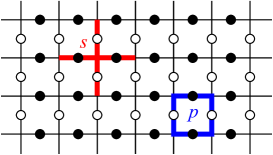
Figure 1: (Color online) Illustration of the square lattice with physical spins on the horizontal (black circles) and the vertical (white circles) edges. Examples of a star ($s$) and a plaquette ($p$) are included.

In the case of $\lambda=0$, the system is exactly solvable because $[\hat{A}_{s},\hat{B}_{p}]=[\hat{A}_{s},\hat{H}(0)]=[\hat{B}_{p},\hat{H}(0)]=0$. The sectors with different sets of expectation values $\{A_{s}\equiv\langle\hat{A}_{s}\rangle=\pm 1\}$ and $\{B_{p}\equiv\langle\hat{B}_{p}\rangle=\pm 1\}$ can be treated independently. In the ground-state sector with $A_{s}=+1$ ($\forall s$) and $B_{p}=+1$ ($\forall p$), there are four linearly independent degenerate ground states that are distinguished by the topological quantum numbers $Z_{1,2}=\pm 1$. These quantum numbers are expectation values for products of $\hat{\sigma}_{i}^{z}$ operators along horizontal and vertical strings going around the lattice. The ground state with $Z_{1}=Z_{2}=+1$ becomes $|0\rangle=\mathcal{N}\prod_{s}(1+\hat{A}_{s})|\Uparrow\,\rangle$, where $\mathcal{N}$ is a normalization constant and $|\Uparrow\,\rangle$ is the completely polarized state with $\sigma_{i}^{z}\equiv\langle\hat{\sigma}_{i}^{z}\rangle=+1$ ($\forall i$).

In the case of $\lambda>0$, the system is not exactly solvable in general because $[\hat{A}_{s},\hat{\sigma}_{i}^{z}]\neq 0$. On the other hand, it is true that $[\hat{B}_{p},\hat{Z}_{1,2}]=[\hat{B}_{p},\hat{H}(\lambda)]=[\hat{Z}_{1,2},\hat{H}(\lambda)]=0$, therefore the sectors with different values of $B_{p}$ and $Z_{1,2}$ can be treated independently. In the following, we only consider the lowest-energy sector with $B_{p}=+1$ ($\forall p$) and $Z_{1}=Z_{2}=+1$. The states within this sector are distinguished by the expectation values $\{A_{s}=\pm 1\}$, and we introduce a corresponding representation with quasi-spins $A_{s}$ located at the stars Dusuel . In this quasi-spin representation, the quasi-spin $A_{s}$ is measured by the operator $\hat{A}_{s}^{z}\equiv\hat{A}_{s}$ and switched by the operator $\hat{A}_{s}^{x}$, therefore the quasi-spin operators $\hat{A}_{s}^{z}$ and $\hat{A}_{s}^{x}$ satisfy the standard spin commutation relations. Note that $\hat{\sigma}_{i}^{z}=\hat{A}_{s}^{x}\hat{A}_{s^{\prime}}^{x}$ for an edge $i$ between two neighboring stars $s$ and $s^{\prime}$. Up to an additive constant, the Hamiltonian in Eq. (1) becomes

$$\hat{H}(\lambda)=-\sum_{s}\hat{A}_{s}^{z}-\lambda\sum_{\langle s,s^{\prime}\rangle\in h}\hat{A}_{s}^{x}\hat{A}_{s^{\prime}}^{x}-\kappa\lambda\sum_{\langle s,s^{\prime}\rangle\in v}\hat{A}_{s}^{x}\hat{A}_{s^{\prime}}^{x},$$ (2)

where $\langle s,s^{\prime}\rangle$ means that the summation is over edges between neighboring stars $s$ and $s^{\prime}$. The TCM with external magnetic field is therefore equivalent to a 2D transverse field Ising model (TFIM) in which the coupling strengths on the horizontal and the vertical edges are not equal in general.

When studying the quantum quench, we are interested in the time evolution of the quantum state $|\Psi(t)\rangle$ after a sudden change in the Hamiltonian. At time $t=0$, the system is set up in the ground state of the initial Hamiltonian $\hat{H}(0)$ such that $|\Psi(0)\rangle=|0\rangle$. At time $t>0$, the system is evolved with the quench Hamiltonian $\hat{H}(\lambda)$ and the state takes the general form $|\Psi(t)\rangle=\exp[-it\hat{H}(\lambda)]|0\rangle$. To extract any valuable information from this expression, we need to obtain a full solution of the Hamiltonian $\hat{H}(\lambda)$. In the following, we consider two important limits. When $\kappa=1$, the horizontal and the vertical coupling strengths are equal, and the equivalent TFIM is the standard 2D TFIM. When $\kappa\rightarrow 0+$, the vertical coupling strength vanishes, and the equivalent TFIM factorizes into $N$ independent 1D TFIM copies along the horizontal chains of the lattice Yu . The $\kappa=0$ case has an exact solution available for all values of $\lambda$, while the $\kappa=1$ case requires perturbation theory around the exactly solvable point at $\lambda=0$.

Topological Rényi entropy.—The Rényi entropy of order $\alpha$ is a generalization of the usual (von Neumann) entanglement entropy that characterizes the quantum entanglement between two complementary subsystems $A$ and $B\equiv\overline{A}$. It is defined by $S_{\alpha}^{AB}\equiv\log_{2}\mathrm{Tr}[\hat{\rho}_{A}^{\alpha}]/(1-\alpha)$, where $\hat{\rho}_{A}$ is the reduced density operator for $A$. Note that the usual entanglement entropy is recovered in the special case of $\alpha=1$.

The topological Rényi entropy is extracted from independent Rényi entropies $S_{\alpha}^{(m)}$ calculated in the four cases $(m)$ of Fig. 2 as $S_{\alpha}^{T}\equiv-S_{\alpha}^{(1)}+S_{\alpha}^{(2)}+S_{\alpha}^{(3)}-S_{\alpha}^{(4)}$. When defining $S_{\alpha}^{T}$ in the standard way TE , we take $S_{\alpha}^{(m)}=S_{\alpha}^{AB}$ between the two thick subsystems $A$ and $B$. However, it was argued in Ref. Halasz that the presence of the $\mathbb{Z}_{2}$ lattice gauge structure due to the constraint $B_{p}=+1$ ($\forall p$) makes it possible to substitute the subsystem $A$ with its boundary $\partial A$. In the following, we use the corresponding modified definition for $S_{\alpha}^{T}$ in which we take $S_{\alpha}^{(m)}=S_{\alpha}^{\partial A,\overline{\partial A}}\equiv S_{\alpha}^{\partial A}$ between the thin boundary subsystem $\partial A$ and the rest of the system. The topological Rényi entropy is non-zero if and only if the given state has topological order. For example, its value is $S_{\alpha}^{T}=2$ for the TCM ground state $|0\rangle$ and $S_{\alpha}^{T}=0$ for the completely polarized state $|\Uparrow\,\rangle$. Note that the dimensions $D$ and $d$ of the subsystems need to be macroscopic such that $D>d\gg 1$.

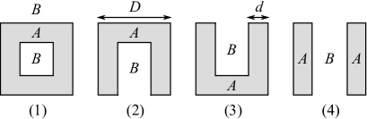
Figure 2: Illustration of the subsystems $A$ and $B$ in the four cases $(m)$ that are used to calculate the topological Rényi entropy.

The modified definition for the topological Rényi entropy is an immense simplification to our calculations because the reduced density matrix $\rho_{\partial A}$ is diagonal in the basis of the physical spins $\sigma_{i}^{z}$. It was shown in Ref. Halasz that if the boundary subsystem $\partial A$ consists of $n$ closed loops with a combined length $L$, the Rényi entropy of order $2$ for a generic state $|\Psi\rangle$ satisfying the gauge constraint $B_{p}=+1$ ($\forall p$) is

$$S_{2}^{\partial A} = (L-n)-\log_{2}\bigg{[}1+\sum_{s_{1},s_{2}}\langle\Psi|\hat{A}_{s_{1}}^{x}\hat{A}_{s_{2}}^{x}|\Psi\rangle^{2}$$ (3)

$$+ \sum_{s_{1},s_{2},s_{3},s_{4}}\langle\Psi|\hat{A}_{s_{1}}^{x}\hat{A}_{s_{2}}^{x}\hat{A}_{s_{3}}^{x}\hat{A}_{s_{4}}^{x}|\Psi\rangle^{2}\ +\ldots\bigg{]},$$

where the sum inside the logarithm contains all $2^{L-n}$ possible products with an even number of quasi-spin operators $\hat{A}_{s}^{x}$ chosen from each closed loop of the subsystem $\partial A$.

Exact treatment.—In the case of $\kappa=0$, there are no interactions between the horizontal chains of the lattice, and the 2D system factorizes into $N$ independent 1D systems in terms of the quasi-spins $A_{s}$. Indeed, the 2D Hamiltonian in Eq. (2) becomes the direct sum of $N$ identical 1D Hamiltonians. If we consider any horizontal chain and label its $N$ stars with $1\leq l\leq N$, the corresponding 1D Hamiltonian is

$$\hat{h}(\lambda)=-\sum_{l=1}^{N}\left(\hat{A}_{l}^{z}+\lambda\hat{A}_{l}^{x}\hat{A}_{l-1}^{x}\right),$$ (4)

where the periodic boundary conditions are taken into account by $A_{0}\equiv A_{N}$. Since the 1D TFIM Hamiltonian in Eq. (4) is exactly solvable by means of a standard procedure Barouch , we can determine the exact time evolution of the Rényi entropy after the quantum quench Supplement . Note that despite the factorization into independent 1D chains in terms of the quasi-spins, this calculation gives the Rényi entropy of a strongly entangled 2D state in terms of the physical spins.

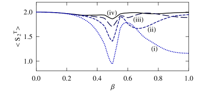
Figure 3: (Color online) Exact long-term time average of $S_{2}^{T}$ as a function of $\beta=\lambda/(1+\lambda)$ for various system sizes: $N=40$ and $D=3d=6$ (i); $N=60$ and $D=3d=9$ (ii); $N=80$ and $D=3d=12$ (iii); $N=100$ and $D=3d=15$ (iv).

The long-term time average of the topological Rényi entropy against the magnetic field $\lambda$ of the quench Hamiltonian $\hat{H}(\lambda)$ is plotted in Fig. 3. The time averages are calculated from $1000$ independent time instants, which are taken from a sufficiently long interval at sufficiently large times such that $t\gg\max\{1,\lambda^{-1}\}$ for all time instants $t$. We first notice that $\langle S_{2}^{T}\rangle$ is distinct from the value of $S_{2}^{T}=0$ that would correspond to the lack of topological order. Instead, it is found for all magnetic fields $\lambda$ that $\langle S_{2}^{T}\rangle$ is close to the initial value of $S_{2}^{T}=2$ and gets closer to it if we increase the system size $N$ as well as the subsystem dimensions $D$ and $d$. We therefore argue that $S_{2}^{T}=2$ in the thermodynamic limit for all times $t$ after a quench with an arbitrary magnetic field $\lambda$.

Perturbation theory.—In the case of $\kappa=1$, the Hamiltonian in Eq. (2) requires perturbation theory around the exactly solvable point at $\lambda=0$. Our aim is to determine the time evolution of the first-order correction to $S_{2}^{T}$. In general, the most straightforward approach is the method of perturbative continuous unitary transformations Halasz ; Dusuel ; PCUT . However, a naive first-order perturbation theory is sufficient in our case, and we derive our results using this simpler approach.

The unperturbed ground state of the initial Hamiltonian $\hat{H}(0)$ is $|0\rangle$ and the perturbed ground state of the quench Hamiltonian $\hat{H}(\lambda)$ is $|\Omega\rangle$. In the first order of perturbation theory, the perturbed ground state takes the expansion form $|\Omega\rangle=|0\rangle+(\lambda/4)\sum_{\langle\mathbf{r_{1}},\mathbf{r_{2}}\rangle}|\{\mathbf{r_{1}},\mathbf{r_{2}}\}\rangle$, where $|\{\mathbf{r_{1}},\mathbf{r_{2}}\}\rangle$ is the state with two star excitations at the positions $\mathbf{r_{1}}$ and $\mathbf{r_{2}}$ such that $A_{\mathbf{r_{1}}}^{z}=A_{\mathbf{r_{2}}}^{z}=-1$. The position of each star is labeled by the 2D vector $\mathbf{r}=(x,y)$ with $0\leq x,y<N$. In terms of the ground state $|\Omega\rangle$, the initial state $|\Psi(0)\rangle$ becomes $|\Psi(0)\rangle=|0\rangle=|\Omega\rangle-(\lambda/4)\sum_{\langle\mathbf{r_{1}},\mathbf{r_{2}}\rangle}|\{\mathbf{r_{1}},\mathbf{r_{2}}\}\rangle$. Although the non-degenerate corrections to the excited states $|\{\mathbf{r_{1}},\mathbf{r_{2}}\}\rangle$ vanish in the first-order calculation, the perturbation introduces a hopping between these degenerate states. The two star excitations can hop between neighboring stars with an amplitude $-\lambda$, and their only interaction is a hard-core repulsion: they are not allowed to be at the same star. However, this interaction is negligible in the thermodynamic limit because the two excitations are far away from each other. The exact eigenstates of the quench Hamiltonian with two star excitations are then $|\mathbf{k_{1}},\mathbf{k_{2}}\rangle=N^{-2}\sum_{\mathbf{r_{1}},\mathbf{r_{2}}}e^{i(\mathbf{K_{1}}\cdot\mathbf{r_{1}}+\mathbf{K_{2}}\cdot\mathbf{r_{2}})}|\{\mathbf{r_{1}},\mathbf{r_{2}}\}\rangle$, where $\mathbf{k}=(k_{x},k_{y})$ with $0\leq k_{x},k_{y}<N$, and each excitation has a 2D momentum $\mathbf{K}=2\pi\mathbf{k}/N$. Note that the state $|\{\mathbf{r_{1}},\mathbf{r_{2}}\}\rangle=|\{\mathbf{r_{2}},\mathbf{r_{1}}\}\rangle$ appears twice in the sum. Since the system and the initial state are both invariant under translations, we only need to consider the eigenstates with zero total momentum $\mathbf{k_{1}}+\mathbf{k_{2}}$. These states labeled by $|\mathbf{k}\rangle\equiv|\mathbf{k},-\mathbf{k}\rangle$ have relative energies $E(\mathbf{k})=4-4\lambda\epsilon(\mathbf{k})$ with respect to the ground state $|\Omega\rangle$, where $\epsilon(\mathbf{k})\equiv\cos(K_{x})+\cos(K_{y})$. In terms of the eigenstates, the initial state $|\Psi(0)\rangle$ takes the form $|\Psi(0)\rangle=|0\rangle=|\Omega\rangle-(\lambda/2)\sum_{\mathbf{k}}^{\prime}\epsilon(\mathbf{k})|\mathbf{k}\rangle$, where the prime means that the summation is only over half of the $N^{2}$ possible $\mathbf{k}$ values. The state $|\Psi(t)\rangle$ after the time evolution with $\hat{H}(\lambda)$ is then obtained by the substitution $\epsilon(\mathbf{k})\rightarrow\epsilon(\mathbf{k})e^{-itE(\mathbf{k})}$, and in terms of the states $|\{\mathbf{r_{1}},\mathbf{r_{2}}\}\rangle$ it reads

$$|\Psi(t)\rangle=|\Omega\rangle+\sum_{(\mathbf{r_{1}},\mathbf{r_{2}})}Q(\mathbf{r_{1}},\mathbf{r_{2}},t)|\{\mathbf{r_{1}},\mathbf{r_{2}}\}\rangle,$$ (5)

where $(\mathbf{r_{1}},\mathbf{r_{2}})$ means that the summation is over pairs of stars without double counting. The coefficient of each state is $Q(\mathbf{r_{1}},\mathbf{r_{2}},t)=-(\lambda/N^{2})\sum_{\mathbf{k}}^{\prime}\epsilon(\mathbf{k})\cos[\mathbf{K}\cdot(\mathbf{r_{1}}-\mathbf{r_{2}})]e^{-itE(\mathbf{k})}$. Since the functions $Q(\mathbf{r_{1}},\mathbf{r_{2}},t)$ consist of many incoherent oscillations with different frequencies $E(\mathbf{k})$, the average modulus square of any such function is given by

$$\big{\langle}|Q(\mathbf{r_{1}},\mathbf{r_{2}},t)|^{2}\big{\rangle}=\frac{\lambda^{2}}{N^{4}}\sum_{\mathbf{k}}^{\prime}\epsilon(\mathbf{k})^{2}\cos^{2}\big{[}\mathbf{K}\cdot(\mathbf{r_{1}}-\mathbf{r_{2}})\big{]}=\frac{\lambda^{2}}{4N^{2}}\,.$$ (6)

This result has a simple physical interpretation. The two excitations are always at neighboring stars before the time evolution, and the sum of the norm squares in the states with two excitations is $2N^{2}\lambda^{2}/16=N^{2}\lambda^{2}/8$ because there are $2N^{2}$ ways of choosing two neighboring stars. During the time evolution, the excitations hop between stars, and the norm square is distributed uniformly between all possible states with two star excitations. Since there are $N^{2}(N^{2}-1)/2\approx N^{4}/2$ ways of choosing any two stars, the uniform norm square corresponds to the result $\lambda^{2}/4N^{2}$ in Eq. (6).

When calculating the Rényi entropy for the state $|\Psi(t)\rangle$ in Eq. (5), there are two corrections to the value $S_{2}^{\partial A}=L-n$ for the unperturbed ground state $|0\rangle$: a static correction from the perturbed ground state $|\Omega\rangle$ and a dynamic correction from the oscillating terms $\propto Q(\mathbf{r_{1}},\mathbf{r_{2}},t)$. The static correction is linearly proportional to the combined length $L$ of the boundary in each case $(m)$, therefore its topological contribution vanishes Halasz . On the other hand, the terms $\propto Q(\mathbf{r_{1}},\mathbf{r_{2}},t)$ give an expectation value $\langle\Psi(t)|\hat{A}_{\mathbf{r_{1}}}^{x}\hat{A}_{\mathbf{r_{2}}}^{x}|\Psi(t)\rangle=2\,\mathrm{Re}[Q(\mathbf{r_{1}},\mathbf{r_{2}},t)]$ for each pair of stars $\mathbf{r_{1}}$ and $\mathbf{r_{2}}$ on the same closed loop of the boundary. Since $\langle\textrm{Re}[Q(\mathbf{r_{1}},\mathbf{r_{2}},t)]^{2}\rangle=\langle|Q(\mathbf{r_{1}},\mathbf{r_{2}},t)|^{2}\rangle/2$ and there are $\ell(\ell-1)/2$ ways of choosing two stars from a closed loop of length $\ell$, the time average of the dynamic correction is $\langle\Delta S_{2}^{\partial A}\rangle=-\lambda^{2}\ell(\ell-1)/(4N^{2}\ln 2)$ for each closed loop of the boundary in each case $(m)$. Since there is a term $\propto\ell^{2}$, the topological contribution does not vanish, and the resulting time average of the topological Rényi entropy is

$$\langle S_{2}^{T}\rangle=2-\frac{\lambda^{2}\left(8D^{2}-16d^{2}\right)}{N^{2}\ln 2}\,.$$ (7)

If we take both the system size and the subsystem dimensions to infinity such that $D\sim d\sim N^{1/4}$, the perturbative correction vanishes as $N^{-3/2}$. We can thus choose macroscopic subsystems in the thermodynamic limit such that the topological Rényi entropy is $S_{2}^{T}=2$ for all times $t$.

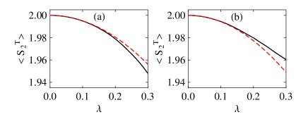
Figure 4: (Color online) Long-term time average of $S_{2}^{T}$ from the exact treatment (solid black line) and the first-order perturbation theory (dashed red line) for two system sizes: $N=40$ and $D=3d=6$ (a); $N=80$ and $D=3d=12$ (b).

To verify that the first-order perturbation theory is indeed a good approximation at $\lambda\ll 1$ and is not invalidated by higher-order corrections, we also establish an analogous perturbation theory in the exactly solvable $\kappa=0$ case. The first-order time average of the topological Rényi entropy takes the form

$$\langle S_{2}^{T}\rangle=2-\frac{\lambda^{2}\left(d^{2}+6D-6d-1\right)}{2N\ln 2}\,.$$ (8)

Note that the correction in this case vanishes as $N^{-1/2}$ when $D\sim d\sim N^{1/4}$. The exact results and those obtained from the perturbation theory are plotted together in Fig. 4. We notice that the respective curves are in good agreement when $\lambda\ll 1$, and therefore we argue that the first-order perturbation theory is a good approximation in the $\kappa=1$ case as well.

Conclusions.—In this Letter, we studied the resilience of topological order in the TCM ground state after a quantum quench with an external magnetic field. The time evolution of topological order was detected via the topological Rényi entropy of order $2$. We considered two different quenches: the integrable one was solved exactly, while the non-integrable one was treated with perturbation theory. In both cases, we found that topological order is resilient in the thermodynamic limit. Our results are in agreement with those in Ref. Tsomokos , but they apply to significantly larger system sizes.

It is interesting to discuss the generic conditions under which topological order is resilient. First of all, the results for the non-integrable quench show that integrability does not play a role. On the other hand, both quenches preserve the $\mathbb{Z}_{2}$ gauge structure of the TCM ground state. This gauge structure allows us to use the modified definition for $S_{2}^{T}$, which in turn makes the subsequent calculations possible. We therefore believe that topological order characterized by $S_{2}^{T}$ is a robust non-equilibrium property of the system whenever gauge invariance is preserved. In perspective, it would be important to study the behavior of topological order after a more generic non-gauge-preserving quench. This further step could help us better understand the universal non-equilibrium and thermal properties of topologically ordered systems.

We thank X.-G. Wen for illuminating discussions. This work was supported in part by the National Basic Research Program of China Grants No. 2011CBA00300 and No. 2011CBA00301 and the National Natural Science Foundation of China Grants No. 61073174, No. 61033001, and No. 61061130540. Research at the Perimeter Institute for Theoretical Physics is supported in part by the Government of Canada through NSERC and by the Province of Ontario through MRI.

References

- (1) X.-G. Wen, Quantum Field Theory of Many-Body Systems (Oxford University Press, Oxford, 2004).
- (2) A. Y. Kitaev, Ann. Phys. (Amsterdam) 303, 2 (2003).
- (3) M. H. Freedman, A. Kitaev, and Z. Wang, Commun. Math. Phys. 227, 587 (2002); C. Nayak, S. H. Simon, A. Stern, M. Freedman, and S. Das Sarma, Rev. Mod. Phys. 80, 1083 (2008).
- (4) A. Hamma, R. Ionicioiu, and P. Zanardi, Phys. Lett. A 337, 22 (2005); A. Hamma, R. Ionicioiu, and P. Zanardi, Phys. Rev. A 71, 022315 (2005).
- (5) A. Kitaev and J. Preskill, Phys. Rev. Lett. 96, 110404 (2006); M. Levin and X.-G. Wen, ibid. 96, 110405 (2006).
- (6) S. T. Flammia, A. Hamma, T. L. Hughes, and X.-G. Wen, Phys. Rev. Lett. 103, 261601 (2009).
- (7) I. H. Kim, Phys. Rev. B 86, 245116 (2012).
- (8) A. Hamma, W. Zhang, S. Haas, and D. A. Lidar, Phys. Rev. B 77, 155111 (2008).
- (9) S. V. Isakov, M. B. Hastings, and R. G. Melko, Nat. Phys. 7, 772 (2011).
- (10) L. Amico, R. Fazio, A. Osterloh, and V. Vedral, Rev. Mod. Phys. 80, 517 (2008).
- (11) P. Zanardi and L. C. Venuti, arXiv:1205.2507.
- (12) G. B. Halász and A. Hamma, Phys. Rev. A 86, 062330 (2012).
- (13) P. Horodecki and A. Ekert, Phys. Rev. Lett. 89, 127902 (2002); M. B. Hastings, I. González, A. B. Kallin, and R. G. Melko, ibid. 104, 157201 (2010); S. J. van Enk and C. W. J. Beenakker, ibid. 108, 110503 (2012); D. A. Abanin and E. Demler, ibid. 109, 020504 (2012).
- (14) A. Polkovnikov, K. Sengupta, A. Silva, and M. Vengalattore, Rev. Mod. Phys. 83, 863 (2011).
- (15) M. Greiner, O. Mandel, T. Esslinger, T. W. Hänsch, and I. Bloch, Nature (London) 415, 39 (2002); M. Greiner, O. Mandel, T. W. Hänsch, and I. Bloch, Nature (London) 419, 51 (2002).
- (16) P. Calabrese and J. Cardy, Phys. Rev. Lett. 96, 136801 (2006); M. A. Cazalilla, ibid. 97, 156403 (2006); M. Rigol, V. Dunjko, V. Yurovsky, and M. Olshanii, ibid. 98, 050405 (2007); A. Rahmani and C. Chamon, Phys. Rev. B 82, 134303 (2010).
- (17) D. I. Tsomokos, A. Hamma, W. Zhang, S. Haas, and R. Fazio, Phys. Rev. A 80, 060302(R) (2009).
- (18) S. Dusuel, M. Kamfor, K. P. Schmidt, R. Thomale, and J. Vidal, Phys. Rev. B 81, 064412 (2010).
- (19) J. Yu, S.-P. Kou, and X.-G. Wen, Europhys. Lett. 84, 17004 (2008).
-
(20)
E. Barouch, B. M. McCoy, and M. Dresden, Phys.
Rev. A 2, 1075 (1970); E. Barouch and B. M. McCoy,
ibid. 3, 786 (1971).
- (21) See Supplemental Material at http://link.aps.org/supplemental/ 10.1103/PhysRevLett.110.170605 for details.
- (22) F. Wegner, Ann. Phys. (Berlin) 506, 77 (1994); S. D. Głazek and K. G. Wilson, Phys. Rev. D 48, 5863 (1993); S. D. Głazek and K. G. Wilson, ibid. 49, 4214 (1994); S. Dusuel and J. Vidal, Phys. Rev. B 71, 224420 (2005); S. Dusuel, M. Kamfor, R. Orús, K. P. Schmidt, and J. Vidal, Phys. Rev. Lett. 106, 107203 (2011).