Abstract

A new definition of Lie invariance for nonlinear multi-dimensional boundary value problems (BVPs) is proposed by the generalization of known definitions to much wider classes of BVPs. The class of (1+3)-dimensional nonlinear BVPs of the Stefan type, modeling the process of melting and evaporation of metals, is studied in detail. Using the definition proposed, the group classification problem for this class of BVPs is solved and some reductions (with physical meaning) to BVPs of lower dimensionality are made. Examples of how to construct exact solutions of the (1+3)-dimensional nonlinear BVP with the correctly-specified coefficients are presented.

1 Introduction

Currently, Lie symmetries are widely applied to study partial differential equations (PDEs) (including multi-component systems of multi-dimensional PDEs), notably, for their reductions to ordinary differential equations (ODEs) and constructing exact solutions. There are a vast number of papers and many excellent books (see, e.g., [1, 2, 3, 4, 5] and references cited therein) devoted to such applications. However, one may note that the authors usually do not pay any attention to the application of Lie symmetries for solving boundary value problems (BVPs). To the best of our knowledge, the first papers that did so were published at the beginning of 1970s (see [6] and [7] and their extended versions presented in books [8] and [2], respectively). The books, which highlight essential role of Lie symmetries in solving BVPs and present several examples, were published much later [2, 9, 10].

The main object of this paper is a class of (1+3)-dimensional nonlinear BVPs of the Stefan type. These problems are widely used in mathematical modeling of a wide range of processes, which arise in physics, biology, chemistry and industry [11, 12, 13, 15, 16, 14]. Nevertheless, these processes can be very different from the formal point of view, they have the common peculiarity, unknown moving boundaries (free boundaries). Movement of unknown boundaries is described by the famous Stefan boundary conditions [17, 16, 18]. It is well known that exact solutions of BVPs of the Stefan type can be derived only in exceptional cases and the relevant list is not very long at the present time (see [11, 23, 22, 19, 20, 21, 25, 26, 24] and references cited therein). Notably, those exact solutions were constructed under additional conditions on their form and/or the coefficients arising in the relevant BVP. It should also be stressed that all analytical results derived in those papers are concerned with two-dimensional BVPs. To the best of our knowledge, there are no invariant solutions (with physical meaning) of multidimensional BVPs with free boundaries excepting particular problems with radial symmetry, for which analytical solutions are found (see, e.g., [11, 27] and references cited therein). Perhaps [28] (see also references by the same author cited therein) is unique because it contains such exact solutions for (1+3)-dimensional hydrodynamical problems with free boundaries. Of course, there are many interesting papers, devoted to the rigorous asymptotic analysis of such BVPs, leading to the relevant analytical results (see,e.g., [29, 30, 31] and references cited therein).

From the mathematical point of view, BVPs with free boundaries are more complicated objects than the standard BVPs with fixed boundaries. In a particular case, each BVP with Stefan boundary conditions is nonlinear; nevertheless, the basic equations may be linear [16, 32]. Thus, the classical methods of solving linear BVPs (the Fourier method, the Laplace transformation and so forth) cannot be directly applied for solving any BVP with free boundaries. On the other hand, it can be noted that the Lie symmetry method can be more applicable just for solving problems with moving boundaries than for other BVPs. In fact, the structure of unknown boundaries may depend on invariant variable(s) and this provides the possibility to reduce the BVP in question to that of lover dimensionality. This is the reason why some authors have applied the Lie symmetry method to BVPs with free boundaries [7, 6, 33, 28, 34, 24, 35].

The paper is organized as follows. In section 2, we propose a new definition of Lie invariance for any BVPs with basic evolution equations, which generalize the known definitions, and formulate the algorithm for solving the group classification problem. In section 3, we apply the definition and the algorithm to the class of (1+3)-dimensional BVPs of the Stefan type, used to describe melting and evaporation of materials in the case when their surface is exposed to a powerful flux of energy. The main result is presented in Theorem 2, which is a highly non-trivial generalization of that, derived for two-dimensional BVPs in [24] . In section 4, all possible systems of subalgebras (optimal systems of subalgebras) for a subclass of (1+3)-dimensional BVPs admitting a five-dimensional Lie algebra of invariance are constructed. We reduce such problems to the two-dimensional BVPs via the non-conjugate two-dimensional subalgebra. Moreover, we show that this reduction admits a clear physical interpretation. Examples of how to construct exact solutions of the (1+3)-dimensional nonlinear BVP with the specified coefficients of diffusion are presented too. Finally, we present conclusions in section 5.

2 Definition of Lie invariance for a BVP with free boundaries

Consider a BVP for a system of $n$ evolution equations ($n\geq 2$) with $m+1$ independent $(t,x)$ (hereafter $x=(x_{1},x_{2},\ldots,x_{m})$) and $n$ dependent $u=(u_{1},u_{2},\ldots,u_{n})$ variables. Let us assume that the basic equations possess the form

$$u_{t}^{i}=F^{i}\left(x,u,u_{x},\ldots,u_{x}^{(k_{i})}\right),\ i=1,\ldots,n$$ (1)

and are defined on a domain $(0,+\infty)\times{\Omega}\subset\mathbb{R}^{m+1}$, where ${\Omega}$ is an open domain with smooth boundaries. Hereafter, the lower subscripts $t$ and $x$ denote differentiation with respect to these variables and $u_{x}^{(k_{i})}$ denotes a totality of partial derivatives with respect to $x$ of order $k_{i}$ (for example, $u_{x}^{(1)}=u_{x_{1}},\ldots,u_{x_{m}}$).

Consider three types of boundary and initial conditions, which widely arise in applications:

$$s_{a}(t,x)=0:\ B^{j}_{a}\left(t,x,u,u_{x},\ldots,u_{x}^{(k_{a}^{j})}\right)=0,\ a=1,\ldots,p,\,j=1,\ldots,n_{a},$$ (2)

$$S_{b}(t,x)=0:\ B^{l}_{b}\left(t,x,u,\ldots,u_{x}^{(k_{b}^{l})},S_{b}^{(1)},\ldots,S^{(K^{l}_{b})}_{b}\right)=0,\ b=1,\ldots,q,\,l=1,\ldots,n_{b},$$ (3)

and

$$\gamma_{c}(t,x)=\infty:\ \Gamma^{m}_{c}\left(t,x,u,u_{x},\ldots,u_{x}^{(k_{c}^{m})}\right)=0,\ c=1,\ldots,r,\,m=1,\ldots,n_{c}.$$ (4)

Here $k_{a}^{j}<k=\max\{k_{1},\ldots,k_{n}\},\ k_{b}^{l}<k,\ k_{c}^{m}<k$ and $K^{l}_{b}$ are the given numbers, $s_{a}(t,x)$ and $\gamma_{c}(t,x)$ are the known functions, while the functions $S_{b}(t,x)$ defining free boundary surfaces must be found. In (3), the function $S^{(K^{l}_{b})}_{b}$ denotes a totality of derivatives with respect to $t$ and $x$ of order $K^{l}_{b}$ (for instance, $S_{b}^{(1)}=\frac{\partial S_{b}}{\partial t},\frac{\partial S_{b}}{\partial x_{1}},\ldots,\frac{\partial S_{b}}{\partial x_{m}}$). We also assume that all functions arising in (1)–(4) are sufficiently smooth so that a classical solution exists for this BVP.

We note that boundary conditions (4) essentially differ from those (2) because they are defined on the non-regular manifolds ${\cal{M}}_{c}=\{\gamma_{c}(t,x)=\infty\}$. Such conditions appears if one considers BVPs in the unbounded domains and often leads to difficulties. For example, one may check that the definition of BVP invariance presented in [2, 1] is not valid for such conditions.

Consider an $N$–parameter (local) Lie group $G_{N}$ of point transformations of variables $(t,x,u)$ in the Euclidean space $\mathbb{R}^{n+m+1}$ (open subset of $\mathbb{R}^{n+m+1}$) defined by the equations

$$t^{\ast}=T(t,x,\varepsilon),\ \ x^{\ast}_{i}=X_{i}(t,x,\varepsilon),\ \ u^{\ast}_{j}=U_{j}(t,x,u,\varepsilon),\ i=1,\ldots,m,\ j=1,\ldots,n,$$ (5)

where $\varepsilon=(\varepsilon_{1},\varepsilon_{2},\ldots,\varepsilon_{N})$ are the group parameters. According to the general Lie group theory, one may construct the corresponding $N$-dimensional Lie algebra $L_{N}$ with the basic generators

$$X_{\alpha}=\xi^{0}_{\alpha}\frac{\partial}{\partial t}+\xi^{1}_{\alpha}\frac{\partial}{\partial x_{1}}+\ldots+\xi^{m}_{\alpha}\frac{\partial}{\partial x_{m}}+\eta^{1}_{\alpha}\frac{\partial}{\partial u_{1}}+\ldots+\eta^{n}_{\alpha}\frac{\partial}{\partial u_{n}},\ \alpha=1,2,\ldots,N,$$ (6)

where $\xi^{0}_{\alpha}=\left.\frac{\partial T(t,x,\varepsilon)}{\partial\varepsilon_{\alpha}}\right|_{\varepsilon=0},\ \xi^{i}_{\alpha}=\left.\frac{\partial X_{i}(t,x,\varepsilon)}{\partial\varepsilon_{\alpha}}\right|_{\varepsilon=0},\ \eta^{j}_{\alpha}=\left.\frac{\partial U_{j}(t,x,u,\varepsilon)}{\partial\varepsilon_{\alpha}}\right|_{\varepsilon=0}$.

In the extended space $\mathbb{R}^{n+m+q+1}$ of the variables $(t,x,u,S)$ (hereafter $S=(S_{1},...,S_{q})$ ), the Lie algebra $L_{N}$ defines the Lie group $\widetilde{G}_{N}$:

$$t^{\ast}=T(t,x,\varepsilon),\ x_{i}^{\ast}=X_{i}(t,x,\varepsilon),\ u^{\ast}_{j}=U_{j}(t,x,u,\varepsilon),\ S^{\ast}_{b}=S_{b},$$ (7)

where $i=1,\ldots,m,\ j=1,\ldots,n,\ b=1,\ldots,q$.

Now we propose a new definition, which is based on the standard definition of differential equation invariance as an invariant manifold ${\cal{M}}$ [4] and generalizes the previous definitions of BVP invariance (see, e.g., [33, 2, 1, 36]).

Definition 1

The BVP of the form (1)–(4) is called invariant with respect to the Lie group $\widetilde{G}_{N}$ (7) if

• the manifold determined by equation (1) in the space of variables $\left(t,x,u,\ldots,u_{x}^{(k)}\right)$ is invariant with respect to the $k$th-order prolongation of the group $G_{N}$;

• each manifold determined by conditions (2) with any fixed number $a$ is invariant with respect to the $k_{a}$th-order prolongation of the group $G_{N}$ in the space of variables $\left(t,x,u,\ldots,u_{x}^{(k_{a})}\right)$ , where $k_{a}=\max\{k_{a}^{j},\ j=1,\ldots,n_{a}\}$;

• each manifold determined by conditions (3) with any fixed number $b$ is invariant with respect to the $k_{b}$th-order prolongation of the group $\widetilde{G}_{N}$ in the space of variables $\left(t,x,u,\ldots,u_{x}^{(k_{b})},S_{b},\ldots,S^{(k_{b})}_{b}\right)$ , where $k_{b}=\max\{k_{b}^{l},\ K_{b}^{l},\ l=1,\ldots,n_{b}\}$;

• each manifold determined by conditions (4) with any fixed number $c$ is invariant with respect to the $k_{c}$th-order prolongation of the group $G_{N}$ in the space of variables $\left(t,x,u,\ldots,u_{x}^{(k_{c})}\right)$ , where $k_{c}=\max\{k_{c}^{m},\ m=1,\ldots,n_{c}\}$.

Definition 2

The functions $u_{j}=\Phi_{j}(t,x),\,j=1,\ldots,n$ and $S_{b}=\Psi_{b}(t,x),\,b=1,\ldots,q$ form an invariant solution $(u,S)$ of the BVP of the form (1)–(4) corresponding to the Lie group (7) if

• $(u,S)$ satisfies equations (1) and conditions (1)–(4);

• the manifold ${\cal{M}}=\{u_{j}=\Phi_{j}(t,x),\ j=1,\ldots,n;\,S_{b}=\Psi_{b}(t,x),\ b=1,\ldots,q\}$ is an invariant manifold of the Lie group (7).

Remark 1

Definition 1 can be straightforwardly generalized on BVPs with governing systems of equations of hyperbolic, elliptic and mixed types. However, one should additionally assume that $n$-component governing system of PDEs is presented in a ’canonical’ form (some authors uses the natation ’involution form’ in this context), i.e. one possesses the simplest form and there are no non-trivial differential consequences.

If the system of differential equations contain arbitrary functions as coefficients (formally speaking, they can be constants), the group classification problem arises. Such problems was formulated and solved for a class of non-linear heat equations (NHEs) in a pioneering work [37] (see also [5]). At the present time, there are algorithms for rigorous solving group classification problems (see, e.g., [38] and references cited therein), which were successfully applied to different classes of PDEs. Thus, if system (1) and/or the boundary conditions (2)–(4) contain arbitrary functions as coefficients, then we should formulate and solve the group classification problem for the BVP of the form (1)–(4).

We propose the following algorithm of the group classification for the class of BVPs (1)–(4):

• to construct the equivalence group $E_{\mathrm{eq}}$ of local transformations, which transform the governing system of equations into itself;

• to extend the space of $E_{\mathrm{eq}}$ action on the variables $S=(S_{1},...,S_{q})$ by adding the identity transformations for them (see the last formula in (7)) and to denote the group obtained as $\widetilde{E}_{\mathrm{eq}}$;

• to find the equivalence group $\widetilde{E}_{\mathrm{eq}}^{\mathrm{BVP}}$ of local transformations, which transform the class of BVPs (1)–(4) into itself, one extends the space of the $\widetilde{E}_{\mathrm{eq}}$ action on the prolonged space, where all arbitrary elements arising in boundary conditions (2)–(4) are treated as new variables.

• to perform the group classification of the governing system (1) up to local transformations generated by the group $\widetilde{E}_{\mathrm{eq}}^{\mathrm{BVP}}$;

• using Definition 1, to find the principal group of invariance $\widetilde{G}^{0}$, which is admitted by each BVP belonging to the class in question;

• using Definition 1 and the results obtained at step (IV), to describe all possible $\widetilde{E}_{\mathrm{eq}}^{\mathrm{BVP}}$-inequivalent BVPs of the form (1)–(4) admitting maximal invariance groups of higher dimensionality than $\widetilde{G}^{0}$.

3 Lie invariance of a class of (1+3)-dimensional nonlinear BVPs with free boundaries

3.1 Mathematical model of melting and evaporation under a powerful flux of energy

Consider the process of melting and evaporation in half-space $\Omega=\{\textbf{x}=(x_{1},x_{2},x_{3}):x_{3}>0\}$ occupied by a solid material, when its surface (initially it is the plane $x_{3}=0$) is exposed to a powerful flux of energy. We neglect the initial short-time non-equilibrium stage of the process and consider the process at the stage when three phases already take place and assume that this occurs at any moment $t\in\mathfrak{T}=(t_{\ast},+\infty)$, where $t_{\ast}$ is a positive real number. Thus, the heat transfer domain $\Omega(t)=\Omega\times\mathfrak{T}$ consists of three sub-domains occupied by the gas, liquid and solid phases, which will be denoted by $\Omega_{0}(t)$, $\Omega_{1}(t)$ and $\Omega_{2}(t),$ respectively, and the phase division boundary surfaces, $S_{1}(t,\textbf{x})=0$ and $S_{2}(t,\textbf{x})=0$ (see Fig.1). In other words, the domain $\Omega(t)$ admits the disjoint decomposition

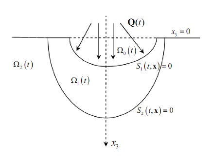
Figure 1: A scheme for the process of melting and evaporation of a solid material which is exposed to a powerful energy flux.

$$\Omega(t)=\Omega_{0}(t)\cup\Gamma_{1}(t)\cup\Omega_{1}(t)\cup\Gamma_{2}(t)\cup\Omega_{2}(t),$$

where

$$\Gamma_{k}(t)=\{(t,\textbf{x}):S_{k}(t,\textbf{x})=0,\ t\in\mathfrak{T},\ \textbf{x}\in\Omega\},\ k=1,2,$$

$$\Omega_{0}(t)=\{(t,\textbf{x}):S_{1}(t,\textbf{x})<0,\ S_{2}(t,\textbf{x})<0,\ t\in\mathfrak{T},\ \textbf{x}\in\Omega\},$$

$$\Omega_{1}(t)=\{(t,\textbf{x}):S_{1}(t,\textbf{x})>0,\ S_{2}(t,\textbf{x})<0,\ t\in\mathfrak{T},\ \textbf{x}\in\Omega\},$$

$$\Omega_{2}(t)=\{(t,\textbf{x}):S_{1}(t,\textbf{x})>0,\ S_{2}(t,\textbf{x})>0,\ t\in\mathfrak{T},\ \textbf{x}\in\Omega\}.$$

Let us consider a class of (1+3)-dimensional nonlinear BVPs of the Stefan type used to describe melting and evaporation of materials in the case when their surface is exposed to a powerful flux of energy [14, 15, 18, 39]:

$$\nabla\left(\lambda_{1}(T_{1})\nabla T_{1}\right)=C_{1}(T_{1})\frac{\partial T_{1}}{\partial t},\ \ (t,\textbf{x})\in\Omega_{1}(t),$$ (8)

$$\nabla\left(\lambda_{2}(T_{2})\nabla T_{2}\right)=C_{2}(T_{2})\frac{\partial T_{2}}{\partial t},\ \ (t,\textbf{x})\in\Omega_{2}(t),$$ (9)

$$\qquad S_{1}(t,\textbf{x})=0:\ \lambda_{1}(T_{v})\frac{\partial T_{1}}{\partial\textbf{n}_{1}}=H_{v}\textbf{V}_{1}\cdot\textbf{n}_{1}-\textbf{Q}(t)\cdot\textbf{n}_{1},\ T_{1}=T_{v},$$ (10)

$$\qquad S_{2}(t,\textbf{x})=0:\ \lambda_{2}(T_{m})\frac{\partial T_{2}}{\partial\textbf{n}_{2}}=\lambda_{1}(T_{m})\frac{\partial T_{1}}{\partial\textbf{n}_{2}}+H_{m}\textbf{V}_{2}\cdot\textbf{n}_{2},\ T_{1}=T_{2}=T_{m},$$ (11)

$$\qquad|\textbf{x}|=+\infty:\ T_{2}=T_{\infty},\ \ t\in\mathfrak{T},$$ (12)

where $T_{v}$, $T_{m}$ and $T_{\infty}$ are the known temperatures of evaporation, melting and solid phases of the material, respectively; $\lambda_{k}(T_{k}),\,k=1,2$ are the positive thermal conductivities; $C_{k}(T_{k})$, $H_{v}$, $H_{m}$ are the positive specific heat values per unit volume; $\textbf{Q}(t)=(Q_{1}(t),Q_{2}(t),Q_{3}(t))$ is the energy flux being absorbed by the material; $S_{k}(t,\textbf{x})=0,\,k=1,2$ are the phase division boundary surfaces to be found; $\textbf{V}_{k}(t,\textbf{x}),\,k=1,2$ are the phase division boundary velocities; $\textbf{n}_{k},\,k=1,2$ are the unit outward normals to the surfaces $S_{k}(t,\textbf{x})=0,\,k=1,2$; $T_{k}(t,\textbf{x}),\,k=1,2$ are the unknown temperature fields; $\nabla=\left(\frac{\partial}{\partial x_{1}},\frac{\partial}{\partial x_{2}},\frac{\partial}{\partial x_{3}}\right)$; the subscripts $k=1$ and $k=2$ correspond to the liquid and solid phases, respectively.

Here equations (8) and (9) are basic and describe the heat transfer process in liquid and solid phases, the boundary conditions (10) present evaporation dynamics on the surface $S_{1}=0$, and the boundary conditions (11) are the well-known Stefan conditions on the surface $S_{2}=0$ dividing the liquid and solid phases. Since the liquid phase thickness is considerably less than the solid phase thickness, one may use the Dirichlet condition (12), where $T_{\infty}$ can be treated as the initial temperature of material. We also assume that the gas phase does not interact with liquid and solid phases; hence the problem in question does not involve any equation for the gas phase.

From the mathematical and physical points of view, we should impose the same additional conditions on the functions and constants arising in the BVP class in question, which guarantee existing classical solutions. Namely, we assume that all functions in (8)–(12) are sufficiently smooth; the free boundary surfaces $S_{k}(t,\textbf{x})=0$ satisfy the restrictions $\frac{\partial S_{k}}{\partial t}\neq 0$ and $|\nabla S_{k}|\neq 0$, $k=1,2$; the projection of the heat flux vector $\textbf{Q}(t)$ on the normal $\textbf{n}_{1}$ is nonzero, i.e. $\textbf{Q}(t)\cdot\textbf{n}_{1}\neq 0$, and $\textbf{V}_{k}\cdot\textbf{n}_{k}\neq~{}0,\ k=1,2$. Finally, the constants $T_{v}$, $T_{m}$ and $T_{\infty}$ satisfy the natural inequalities $T_{v}>T_{m}>T_{\infty}$.

First of all, we simplify the governing system of equations (8) and (9) using the Goodman substitution [40, 41]

$$u=\phi_{1}(T_{1})\equiv\int\limits_{0}^{T_{1}}{C_{1}(\zeta)}\,d\zeta,\quad v=\phi_{2}(T_{2})\equiv\int\limits_{0}^{T_{2}}{C_{2}(\xi)}\,d\xi.$$ (13)

Substituting (13) into (8)–(12) and making the relevant calculations, we arrive at the equivalent class of BVPs

$$\frac{\partial u}{\partial t}=\nabla\left(d_{1}(u)\nabla u\right),\ \ (t,\textbf{x})\in\Omega_{1}(t),$$ (14)

$$\frac{\partial v}{\partial t}=\nabla\left(d_{2}(v)\nabla v\right),\ \ (t,\textbf{x})\in\Omega_{2}(t),$$ (15)

$$\qquad S_{1}(t,\textbf{x})=0:\ d_{1v}\frac{\partial u}{\partial\textbf{n}_{1}}=H_{v}\textbf{V}_{1}\cdot\textbf{n}_{1}-\textbf{Q}(t)\cdot\textbf{n}_{1},\ u=u_{v},$$ (16)

$$\qquad S_{2}(t,\textbf{x})=0:\ d_{2m}\frac{\partial v}{\partial\textbf{n}_{2}}=d_{1m}\frac{\partial u}{\partial\textbf{n}_{2}}+H_{m}\textbf{V}_{2}\cdot\textbf{n}_{2},\ u=u_{m},\ v=v_{m},$$ (17)

$$\qquad|\textbf{x}|=+\infty:\ v=v_{\infty},\ \ t\in\mathfrak{T},$$ (18)

where $u_{v}=\int\limits_{0}^{T_{v}}{C_{1}(\zeta)}\,d\zeta$, $u_{m}=\int\limits_{0}^{T_{m}}{C_{1}(\zeta)}\,d\zeta$, $v_{m}=\int\limits_{0}^{T_{m}}{C_{2}(\xi)}\,d\xi$, $v_{\infty}=\int\limits_{0}^{T_{\infty}}{C_{2}(\xi)}\,d\xi$; $d_{1}(u)=\frac{\lambda_{1}(\phi^{-1}_{1}(u))}{C_{1}(\phi^{-1}_{1}(u))}$, $d_{2}(v)=\frac{\lambda_{2}(\phi^{-1}_{2}(v))}{C_{2}(\phi^{-1}_{2}(v))}$; $d_{1v}=d_{1}(u_{v})$, $d_{1m}=d_{1}(u_{m})$, $d_{2m}=d_{2}(v_{m})$ (here $\phi^{-1}_{k},\,k=1,2$ are the inverse functions of $\phi_{k}$, the functions $d_{1}(u)$ and $d_{2}(v)$ are strictly positive and $u_{v}\neq u_{m}$, $v_{m}\neq v_{\infty}$).

3.2 Group classification of the basic equations (14)–(15)

One sees that the BVP of the form (14)–(18) consists of two standard NHEs with arbitrary smooth functions $d_{1}(u)$ and $d_{2}(v)$ and the boundary conditions (16)–(18) containing an arbitrary vector function $\textbf{Q}(t)$ and a number of arbitrary parameters. Thus, we deal with a class of BVPs, and to carry out the group classification the algorithm formulated in Section 2 can be used.

According to item (I), we need to find the group of equivalent transformations of the non-coupled system of NHEs (14)–(15). Note that this group is well-known in the case of a single NHE (see, e.g., [42]). However, one cannot extend this result in the case of system (14)–(15) in a formal way because the group obtained may be incomplete. Thus, we carefully check the group of equivalent transformations for the non-coupled system (14)–(15).

Lemma 1

The equivalence transformations group $E_{\mathrm{eq}}$ of system (14)–(15) consists of the group $\mathcal{E}_{\mathrm{eq}}$ of continuous equivalence transformations

$$\bar{t}=\alpha t+\gamma_{0},\ \bar{X}=\beta A_{i}(\beta_{1})A_{j}(\beta_{2})A_{k}(\beta_{3})X+\Gamma\ (i,j,k=1,2,3;\ i\neq j,i\neq k,j\neq k),$$

$$\bar{u}=\delta_{1}u+\gamma_{4},\ \bar{v}=\delta_{2}v+\gamma_{5},\ \bar{d}_{1}=\frac{\beta^{2}}{\alpha}\ d_{1},\ \bar{d}_{2}=\frac{\beta^{2}}{\alpha}\ d_{2},$$

and the group of discrete equivalence transformations

• $t\rightarrow-t$,  $x_{i}\rightarrow(-1)^{j}x_{i}\ (i=1,2,3,\,j=0,1)$,  $u\rightarrow-u$,  $v\rightarrow-v$,  $d_{1}\rightarrow-d_{1}$,  $d_{2}\rightarrow-d_{2}$;

• $t\rightarrow t$,  $x_{i}\rightarrow(-1)^{j}x_{i}\ (i=1,2,3,\,j=0,1)$,  $u\rightarrow v$,  $v\rightarrow u$,  $d_{1}\rightarrow d_{2}$,  $d_{2}\rightarrow d_{1}$.

Here $\alpha>0,\beta>0,\beta_{1},\ldots,\beta_{3},\gamma_{0},\ldots,\gamma_{5},\delta_{1}>0,\delta_{2}>0$ are arbitrary constants;

$$A_{1}(\theta)=\left(\begin{array}[]{ccc}\cos\theta&\sin\theta&0\\ -\sin\theta&\cos\theta&0\\ 0&0&1\end{array}\right),A_{2}(\theta)=\left(\begin{array}[]{ccc}\cos\theta&0&\sin\theta\\ 0&1&0\\ -\sin\theta&0&\cos\theta\end{array}\right),A_{3}(\theta)=\left(\begin{array}[]{ccc}1&0&0\\ 0&\cos\theta&\sin\theta\\ 0&-\sin\theta&\cos\theta\end{array}\right)$$

are the matrix of rotation in space, and

$$X=\left(\begin{array}[]{c}x_{1}\\ x_{2}\\ x_{3}\end{array}\right),\ \Gamma=\left(\begin{array}[]{c}\gamma_{1}\\ \gamma_{2}\\ \gamma_{3}\end{array}\right).$$

Proof. To find the group $\mathcal{E}_{\mathrm{eq}}$, we use the standard infinitesimal method [5, 43], i.e., search for the generators of the form

$$Y=\xi^{0}\frac{\partial}{\partial t}+\xi^{a}\frac{\partial}{\partial x_{a}}+\eta^{1}\frac{\partial}{\partial u}+\eta^{2}\frac{\partial}{\partial v}+\mu^{1}\frac{\partial}{\partial d_{1}}+\mu^{2}\frac{\partial}{\partial d_{2}},$$

where $a=1,2,3$ (hereafter, summation is assumed from 1 to 3 over repeated indices $a$ or $b$). The generator $Y$ defines the group $\mathcal{E}_{\mathrm{eq}}$ of equivalence transformations

$$\bar{t}=\phi(t,\textbf{x},u,v),\ \bar{x}_{a}=\psi_{a}(t,\textbf{x},u,v),\ \bar{u}=\Phi_{1}(t,\textbf{x},u,v),\ \bar{v}=\Phi_{2}(t,\textbf{x},u,v),$$

$$\bar{d_{1}}=\Psi_{1}(t,\textbf{x},u,v,d_{1},d_{2}),\ \bar{d_{2}}=\Psi_{2}(t,\textbf{x},u,v,d_{1},d_{2})$$

for the class of systems (14)–(15) iff $Y$ obeys the condition of invariance of the following system:

$$\frac{\partial u}{\partial t}-\nabla\left(d_{1}\nabla u\right)=0,\ \frac{\partial d_{1}}{\partial t}=0,\ \frac{\partial d_{1}}{\partial x_{a}}=0,\ \frac{\partial d_{1}}{\partial v}=0,$$ (19)

$$\frac{\partial v}{\partial t}-\nabla\left(d_{2}\nabla v\right)=0,\ \frac{\partial d_{2}}{\partial t}=0,\ \frac{\partial d_{2}}{\partial x_{a}}=0,\ \frac{\partial d_{2}}{\partial u}=0.$$ (20)

Here, the variables $u$ and $v$ are considered in the space $(t,\textbf{x})$, while $d_{k}$ in the extended space $(t,\textbf{x},u,v)$. The coordinates $\xi^{0},\xi^{a}$ and $\eta^{k}$ of the operator $Y$ are the functions of the variables $t,\textbf{x},u,v$, while the coordinates $\mu^{k}$ are the functions of $t,\textbf{x},u,v,d_{1},d_{2}$. Thus, the invariance criterium for system (19)–(20) is given by the formulae

$$Y^{(2)}\left.\left(\frac{\partial u}{\partial t}-\nabla\left(d_{1}\nabla u\right)\right)\right|_{\cal S}=0,\ Y^{(2)}\left.\left(\frac{\partial d_{1}}{\partial t}\right)\right|_{\cal S}=0,\ Y^{(2)}\left.\left(\frac{\partial d_{1}}{\partial x_{a}}\right)\right|_{\cal S}=0,\ Y^{(2)}\left.\left(\frac{\partial d_{1}}{\partial v}\right)\right|_{\cal S}=0,$$ (21)

$$Y^{(2)}\left.\left(\frac{\partial v}{\partial t}-\nabla\left(d_{2}\nabla v\right)\right)\right|_{\cal S}=0,\ Y^{(2)}\left.\left(\frac{\partial d_{2}}{\partial t}\right)\right|_{\cal S}=0,\ Y^{(2)}\left.\left(\frac{\partial d_{2}}{\partial x_{a}}\right)\right|_{\cal S}=0,\ Y^{(2)}\left.\left(\frac{\partial d_{2}}{\partial v}\right)\right|_{\cal S}=0,$$ (22)

where $S$ is the manifold, defined by system (19)–(20), $Y^{(2)}$ is the second prolongation of the operator $Y$ calculated via the known formulae [5, 43]. Using these formulae and (21)–(22) and carrying out the relevant calculations one obtains the 13-dimensional Lie algebra with the basic operators

$$Y_{1}=\frac{\partial}{\partial t},\ Y_{2}=\frac{\partial}{\partial x_{1}},\ Y_{3}=\frac{\partial}{\partial x_{2}},\ Y_{4}=\frac{\partial}{\partial x_{3}},$$

$$Y_{5}=x_{2}\frac{\partial}{\partial x_{1}}-x_{1}\frac{\partial}{\partial x_{2}},\ Y_{6}=x_{3}\frac{\partial}{\partial x_{1}}-x_{1}\frac{\partial}{\partial x_{3}},\ Y_{7}=x_{3}\frac{\partial}{\partial x_{2}}-x_{2}\frac{\partial}{\partial x_{3}},$$

$$Y_{8}=\frac{\partial}{\partial u},\ Y_{9}=\frac{\partial}{\partial v},\ Y_{10}=u\frac{\partial}{\partial u},\ Y_{11}=v\frac{\partial}{\partial v},$$

$$Y_{12}=t\frac{\partial}{\partial t}-d_{1}\frac{\partial}{\partial d_{1}}-d_{2}\frac{\partial}{\partial d_{2}},\ Y_{13}=x_{a}\frac{\partial}{\partial x_{a}}+2d_{1}\frac{\partial}{\partial d_{1}}+2d_{2}\frac{\partial}{\partial d_{2}}.$$

One easily checks that this algebra generates the group $\mathcal{E}_{\mathrm{eq}}$.

Finally, to obtain the group of equivalence transformations $E_{\mathrm{eq}}$, we should add the discrete transformations 1) and 2) listed in Lemma 1. It is easy to verify by the direct calculations that system (14)–(15) is invariant under these discrete transformations.

The proof is now complete. $\blacksquare$

According to item (II) of the algorithm, we should now construct the group $\widetilde{E}_{\mathrm{eq}}$ by adding the identity transformations $\widetilde{S}_{1}=S_{1},\widetilde{S}_{2}=S_{2}$. To realize item (III), one needs to apply the transformations generated by the group $\widetilde{E}_{\mathrm{eq}}$ to the boundary conditions (16)–(18) and to find the group $\widetilde{E}^{\mathrm{BVP}}_{\mathrm{eq}}$. The result obtained is formulated as follows.

Lemma 2

The class of BVPs (14)–(18) admits the group of equivalence transformations $\widetilde{E}^{\mathrm{BVP}}_{\mathrm{eq}}$:

$$\tilde{t}=\alpha t+\gamma_{0},\ \widetilde{X}=\beta A_{i}(\beta_{1})A_{j}(\beta_{2})A_{k}(\beta_{3})X+\Gamma\ (i,j,k=1,2,3;\ i\neq j,i\neq k,j\neq k),$$

$$\tilde{u}=\delta_{1}u+\gamma_{4},\ \tilde{v}=\delta_{2}v+\gamma_{5},\ \widetilde{S}_{1}=S_{1},\ \widetilde{S}_{2}=S_{2},\ \tilde{d}_{1}=\frac{\beta^{2}}{\alpha}\ d_{1},\ \tilde{d}_{2}=\frac{\beta^{2}}{\alpha}\ d_{2},$$

$$\tilde{d}_{1v}=\frac{\beta}{\delta_{1}}\ d_{1v},\ \tilde{d}_{1m}=\frac{\beta}{\delta_{1}}\ d_{1m},\ \tilde{d}_{2m}=\frac{\beta}{\delta_{2}}\ d_{2m},\ \widetilde{H}_{v}=\frac{\alpha}{\beta}H_{v},\ \widetilde{H}_{m}=\frac{\alpha}{\beta}H_{m},$$

$$\tilde{u}_{v}=\delta_{1}u_{v}+\gamma_{4},\ \tilde{u}_{m}=\delta_{1}u_{m}+\gamma_{4},\ \tilde{v}_{m}=\delta_{2}v_{m}+\gamma_{5},\ \tilde{v}_{\infty}=\delta_{2}v_{\infty}+\gamma_{5}$$

$$\widetilde{Q}=A_{i}(\beta_{1})A_{j}(\beta_{2})A_{k}(\beta_{3})Q\ (i,j,k=1,2,3;\ i\neq j,i\neq k,j\neq k),$$

with arbitrary coefficients $\alpha,\beta,\beta_{1},\ldots,\beta_{3},\gamma_{0},\ldots,\gamma_{5},\delta_{1},\delta_{2}$ obeying only the condition

$$\alpha\beta\delta_{1}\delta_{2}\neq 0.$$

Table 1: Lie algebras of the NHE system (14)–(15) ($k_{1},k_{2},m$ and $n$ are arbitrary non-zero constants, $b<a=1,2,3$; while $\alpha(t,x)$ and $\beta(t,x)$ are arbitrary solutions of the linear heat equations $\alpha_{t}=k_{1}\alpha_{xx}$ and $\beta_{t}=k_{2}\beta_{xx}$, respectively.)

no	$d_{1}(u)$	$d_{2}(v)$	Basic operators of MAI
1.	$\forall$	$\forall$	$AE(1,3)=\langle\partial_{t},\partial_{x_{a}},x_{a}\partial_{x_{b}}-x_{b}\partial_{x_{a}},2t\partial_{t}+x_{a}\partial_{x_{a}}\rangle$
2.	$k_{1}$	$\forall$	$AE(1,3),u\partial_{u},\alpha(t,\textbf{x})\partial_{u}$
3.	$\forall$	$k_{2}$	$AE(1,3),v\partial_{v},\beta(t,\textbf{x})\partial_{v}$
4.	$e^{u}$	$e^{v}$	$AE(1,3),x_{a}\partial_{x_{a}}+2\partial_{u}+2\partial_{v}$
5.	$e^{u}$	$v^{m}$	$AE(1,3),x_{a}\partial_{x_{a}}+2\partial_{u}+\frac{2}{m}v\partial_{v}$
6.	$u^{n}$	$e^{v}$	$AE(1,3),x_{a}\partial_{x_{a}}+\frac{2}{n}u\partial_{u}+2\partial_{v}$
7.	$u^{n}$	$v^{m}$	$AE(1,3),D=x_{a}\partial_{x_{a}}+\frac{2}{n}u\partial_{u}+\frac{2}{m}v\partial_{v}$
8.	$u^{-\frac{4}{5}}$	$v^{-\frac{4}{5}}$	$AE(1,3),|\textbf{x}|^{2}\partial_{x_{b}}-2x_{b}x_{a}\partial_{x_{a}}+5x_{b}u\partial_{u}+5x_{b}v\partial_{v},\,D$ with $m=n=-\frac{4}{5}$
9.	$k_{1}$	$k_{2}$	$AE(1,3),u\partial_{u},v\partial_{v},\alpha(t,\textbf{x})\partial_{u},\beta(t,\textbf{x})\partial_{v},G_{a}=t\partial_{x_{a}}-x_{a}\left(\frac{1}{2k_{1}}u\partial_{u}+\frac{1}{2k_{2}}v\partial_{v}\right)$,
			$\Pi=t^{2}\partial_{t}+tx_{a}\partial_{x_{a}}-\frac{1}{4k_{1}}(|\textbf{x}|^{2}+6k_{1}t)u\partial_{u}-\frac{1}{4k_{2}}(|\textbf{x}|^{2}+6k_{2}t)v\partial_{v}$
10.	$k_{1}$	$k_{1}$	$AE(1,3),u\partial_{u},v\partial_{v},v\partial_{u},u\partial_{v},\alpha(t,\textbf{x})\partial_{u},\beta(t,\textbf{x})\partial_{v},G_{a}$ and $\Pi$ with $k_{2}=k_{1}$

According to item (IV) of the algorithm, we should now perform the group classification of the governing system (14)–(15) up to local transformations generated by the group $\widetilde{E}_{\mathrm{eq}}^{\mathrm{BVP}}$. The result can be presented as follows.

Theorem 1

All possible maximal algebras of invariance (MAIs) (up to equivalent representations generated by transformations from the group $\widetilde{E}^{\mathrm{BVP}}_{\mathrm{eq}}$) of system (14)–(15) for any fixed vector function $(d_{1},d_{2})$ with strictly positive functions $d_{1}(u)$ and $d_{2}(v)$ are presented in Table 1. Any other system of the form (14)–(15) is reduced to one of those with diffusivities from Table 1 by an equivalence transformation from the group $\widetilde{E}^{\mathrm{BVP}}_{\mathrm{eq}}$.

Proof. First of all, we remind the reader that a complete description of Lie symmetries for the class of multi-dimensional nonlinear reaction-diffusion systems

$$\frac{\partial u}{\partial t}=\nabla\left(d_{1}(u)\nabla u\right)+F_{1}(u,v),$$

$$\frac{\partial v}{\partial t}=\nabla\left(d_{2}(v)\nabla v\right)+F_{2}(u,v),$$

where $F_{1}$ and $F_{2}$ are the arbitrary nonzero smooth functions, was obtained in [44, 45] (the case of constant diffusivities) and [46] (the case of non-constant diffusivities). Nevertheless, the detailed examination of the special case $F_{1}=F_{2}=0$ was omitted in the papers [44, 45, 46], we can use the relevant system of the determining equations with $F_{1}=F_{2}=0$ to find all possible MAIs of system (14)–(15). Let us assume that the MAI in question is generated by the infinitesimal operator

$$X=\xi^{0}(t,\textbf{x},u,v)\frac{\partial}{\partial t}+\xi^{a}(t,\textbf{x},u,v)\frac{\partial}{\partial x_{a}}+\eta^{1}(t,\textbf{x},u,v)\frac{\partial}{\partial u}+\eta^{2}(t,\textbf{x},u,v)\frac{\partial}{\partial v},$$

where $\xi^{0},\ \xi^{a},\ \eta^{1}$ and $\eta^{2}$ are the unknown smooth functions. The form of the system of determining equations to find these functions essentially depends on the derivatives $\frac{dd_{1}}{du}$ and $\frac{dd_{2}}{dv}$. Let us consider the most general case $\frac{dd_{1}}{du}\cdot\frac{dd_{2}}{dv}\neq 0$. The relevant system of determining equations has the form (see formulae (11)–(16) with $F_{1}=F_{2}=0$ in [46])

$$\xi^{0}_{x_{a}}=\xi^{0}_{u}=\xi^{0}_{v}=0,\ \xi^{a}_{u}=\xi^{a}_{v}=\eta^{1}_{v}=\eta^{2}_{u}=0,\ a=1,2,3,$$ (23)

$$\xi^{1}_{x_{1}}=\xi^{2}_{x_{2}}=\xi^{3}_{x_{3}},\ \xi^{a}_{x_{b}}+\xi^{b}_{x_{a}}=0,\ b<a=1,2,3,$$ (24)

$$\xi^{0}_{t}=2\xi^{a}_{x_{a}}-\eta^{1}\frac{d}{du}\log d_{1},\ \xi^{0}_{t}=2\xi^{a}_{x_{a}}-\eta^{2}\frac{d}{dv}\log d_{2},\ a=1,2,3,$$ (25)

$$2\frac{\partial^{2}\eta^{1}}{\partial x_{a}\partial u}+2\eta^{1}_{x_{a}}\frac{d}{du}\log d_{1}=\Delta\xi^{a}-\xi^{a}_{t}\left(d_{1}\right)^{-1},\ 2\frac{\partial^{2}\eta^{2}}{\partial x_{a}\partial v}+2\eta^{2}_{x_{a}}\frac{d}{dv}\log d_{2}=\Delta\xi^{a}-\xi^{a}_{t}\left(d_{2}\right)^{-1},$$ (26)

$$2\xi^{a}_{x_{a}}-\xi^{0}_{t}-\eta^{1}_{u}=\eta^{1}_{uu}\left(\frac{d}{du}\log d_{1}\right)^{-1}+\eta^{1}\frac{d}{du}\log\frac{dd_{1}}{du},\ a=1,2,3,$$ (27)

$$2\xi^{a}_{x_{a}}-\xi^{0}_{t}-\eta^{2}_{v}=\eta^{2}_{vv}\left(\frac{d}{dv}\log d_{2}\right)^{-1}+\eta^{2}\frac{d}{dv}\log\frac{dd_{2}}{dv},\ a=1,2,3,$$ (28)

$$\eta^{1}_{t}-\Delta\eta^{1}d_{1}=0,\ \eta^{2}_{t}-\Delta\eta^{2}d_{2}=0.$$ (29)

If $d_{1}(u)$ and $d_{2}(v)$ are the arbitrary smooth functions, then system (23)–(29) can be easily solved resulting the eight-dimensional Lie algebra $AE(1,3)$ with the basic operators

$$P_{t}=\frac{\partial}{\partial t},\ P_{a}=\frac{\partial}{\partial x_{a}},\ J_{ab}=x_{a}P_{b}-x_{b}P_{a},\ D_{0}=2t\frac{\partial}{\partial t}+x_{a}\frac{\partial}{\partial x_{a}},\,b<a=1,2,3.$$

Now, we should find all possible pairs of the function $d_{1}(u)$ and $d_{2}(v)$ leading to extensions of the algebra $AE(1,3)$. It is evident that equations (23) and (25) can be easily solved and the functions

$$\xi^{0}=A(t),\ \xi^{a}=B^{a}(t,x),\ \ a=1,2,3,$$ (30)

$$\eta^{1}=(2B^{a}_{a}-A_{t})\left(\frac{d}{du}\log d_{1}\right)^{-1},\ \eta^{2}=(2B^{a}_{a}-A_{t})\left(\frac{d}{dv}\log d_{2}\right)^{-1},\ \ a=1,2,3$$ (31)

are obtained (here $A$ and $B^{a}$ are the arbitrary functions at the moment). However, the functions $B^{a}$ can be specified using (24) as follows:

$$B^{a}=c_{0a}+c_{ab}x_{b}+k_{a}(t)|\textbf{x}|^{2}-2k_{b}(t)x_{b}x_{a},\ a,b=1,2,3,$$ (32)

where $c_{ab}+c_{ba}=0\,(a\neq b),c_{11}=\ldots=c_{33}$ and $c_{0a},c_{ab},k_{a}(t),k_{b}(t)$ are arbitrary functions.

Substituting formulae (30) and (31) in (27) and (28) we arrive at the system of classification equations to find pairs of the functions $(d_{1},d_{2})$:

$$\frac{d^{2}}{du^{2}}\left(\frac{d}{du}\log d_{1}\right)^{-1}=0,\ \frac{d^{2}}{dv^{2}}\left(\frac{d}{dv}\log d_{2}\right)^{-1}=0,$$ (33)

otherwise, the conditions

$$2B^{a}_{a}-A_{t}=0,\ a=1,2,3,$$ (34)

must hold. However, substituting (32) in conditions (34) and taking into account (26) and (30)–(31) we immediately obtain only the Lie algebra $AE(1,3)$. System (33), which consists of two independent ODEs, can be easy solved:

$$d_{1}(u)=\left\{\begin{array}[]{lll}D_{1}(u+C_{1})^{\alpha_{1}},\\ D_{1}\exp(\alpha_{1}u),\end{array}\right.$$ (35)

$$d_{2}(v)=\left\{\begin{array}[]{lll}D_{2}(v+C_{2})^{\alpha_{2}},\\ D_{2}\exp(\alpha_{1}v),\end{array}\right.$$ (36)

where $D_{k}\neq 0,\ \alpha_{k}\neq 0$ and $C_{k}$ are arbitrary constants ($k=1,2$).

Substitutions the functions $\xi^{0},\xi^{a},\eta^{1}$ and $\eta^{2}$ from (30)–(31) in (26) we arrive at the equations

$$B_{t}^{a}=-\Delta B^{a}\left(5+4\frac{d^{2}}{du^{2}}\log d_{1}\right)\frac{dd_{1}}{du},\ \ B_{t}^{a}=-\Delta B^{a}\left(5+4\frac{d^{2}}{dv^{2}}\log d_{2}\right)\frac{dd_{2}}{dv}.$$

Since the functions $B_{a},\ (a=1,2,3)$ depend only on $t$ and $x$, there are only two possibilities. The first one is $\Delta B^{a}=0$ and then, applying (32), we obtain

$$B^{a}=c_{ab}x_{b}+c_{a0},\ \ c_{ab},c_{a0}\in\mathbb{R}.$$

The second possibility, having $\Delta B^{a}\neq 0$, requires

$$\left(5+4\frac{d^{2}}{du^{2}}\log d_{1}\right)\frac{dd_{1}}{du}=m_{1},\ \ \left(5+4\frac{d^{2}}{dv^{2}}\log d_{2}\right)\frac{dd_{2}}{dv}=m_{2},$$ (37)

where $m_{1}$ and $m_{2}$ are some constants. Using (35)–(36) it is easily seen that conditions (37) can be satisfied only for $m_{1}=m_{2}=0$, and then

$$d_{1}(u)=D_{1}\left(u+C_{1}\right)^{-\frac{4}{5}},\ \ d_{1}(v)=D_{2}\left(v+C_{2}\right)^{-\frac{4}{5}}.$$ (38)

Thus, we have obtained all possible forms of the functions $d_{1}(u)$ and $d_{2}(v)$, namely formulae (35)–(36) and (38), leading to extensions of the invariance algebra $AE(1,3)$ of the nonlinear system (14)–(15), when both diffusivities are non-constant.

Finally, taking into account the point transformations from the group $\widetilde{E}^{\mathrm{BVP}}_{\mathrm{eq}}$, we immediately obtain cases 4–8 from Table 1. Other possibility, when at least one of the functions $d_{1}(u)$ and $d_{2}(v)$ is constant, was examined in a similar way, and cases 2,3 and 9, 10 from Table 1 were obtained.

The proof is now complete. $\blacksquare$

Remark 2

Cases 2 and 5 from Table 1 are equivalent to 3 and 6, respectively, if one takes into account the discrete transformations 2) from the group $E_{\mathrm{eq}}$. However, these transformations do not belong to the $\widetilde{E}^{\mathrm{BVP}}_{\mathrm{eq}}$, because the boundary conditions (16) and (18) are not invariant under them.

3.3 Group classification of the class of BVPs (14)–(18)

We note that each MAI from Table 1 generates the corresponding maximal groups of invariance (MGI) with the transformations, which can be easily derived from the basic generators listed therein. These transformations are well-known and used below.

Taking this into account and according to items (V) and (VI) of the algorithm, we formulate the main theorem giving the complete list of Lie symmetries of the BVP class (14)–(18).

Theorem 2

The BVP of the form (14)–(18), with the arbitrary given functions $d_{1}(u)$, $d_{2}(v)$ ($d_{1}(u)\not=d_{2}(v)$) and $Q_{a}(t),\ a=1,2,3$, is invariant under the three-parameter Lie group (trivial Lie group) presented in case 1 of Table 2. The MGI of any BVP of the form (14)–(18) does not depend on the form of $d_{1}(u)$ and $d_{2}(v)$. There are only five BVPs from class (14)–(18) with the correctly specified functions $Q_{a}(t),\ a=1,2,3$ admitting the MGI of a higher dimensionality, namely: four- or five-parameter Lie groups of invariance (up to equivalent representations generated by equivalence transformations from the group $\widetilde{E}^{\mathrm{BVP}}_{\mathrm{eq}}$). These MGIs and the relevant functions $Q_{a}(t),\ a=1,2,3$ are presented in cases 2–6 of Table 2.

Table 2: Lie invariance of BVP (14)–(18)

no	$Q_{1}(t)$	$Q_{2}(t)$	$Q_{3}(t)$	MGI
1.	$\forall$	$\forall$	$\forall$	$\widetilde{T}_{1},\widetilde{T}_{2},\widetilde{T}_{3}$
2.	$0$	$0$	$q(t)$	$\widetilde{T}_{1},\widetilde{T}_{2},\widetilde{T}_{3},\widetilde{T}_{5}$
3.	$\Theta_{1}(\lambda t)$	$\Theta_{2}(\lambda t)$	$q_{3}$	$\widetilde{T}_{1},\widetilde{T}_{2},\widetilde{T}_{3},\widetilde{T}_{6}$
4.	$\frac{1}{\sqrt{t}}\ \Theta_{1}\left(\frac{1}{2}\lambda\log t\right)$	$\frac{1}{\sqrt{t}}\ \Theta_{2}\left(\frac{1}{2}\lambda\log t\right)$	$\frac{q_{3}}{\sqrt{t}}$	$\widetilde{T}_{1},\widetilde{T}_{2},\widetilde{T}_{3},\widetilde{T}_{7}$
5.	$0$	$0$	$q$	$\widetilde{T}_{0},\widetilde{T}_{1},\widetilde{T}_{2},\widetilde{T}_{3},\widetilde{T}_{5}$
6.	$0$	$0$	$\frac{q}{\sqrt{t}}$	$\widetilde{T}_{1},\widetilde{T}_{2},\widetilde{T}_{3},\widetilde{T}_{4},\widetilde{T}_{5}$

Remark 3

In Table 2, the following designations are used: $q\neq 0$, $q_{3}$, $\lambda$ are arbitrary constants, $q(t)\neq 0$ is an arbitrary function while the functions

$$\Theta_{1}(\tau)=q_{1}\cos{\tau}+q_{2}\sin{\tau},\ \ \Theta_{2}(\tau)=-q_{1}\sin{\tau}+q_{2}\cos{\tau},$$

where $q_{1}$, $q_{2}$ are arbitrary constants satisfying the condition $q_{1}^{2}+q_{2}^{2}\neq 0$ if $\tau\neq 0$.

The explicit form of the transformations generating the MGI are:

$$\widetilde{T}_{0}:t^{\ast}=t+\varepsilon_{0},\ x_{1}^{\ast}=x_{1},\ x_{2}^{\ast}=x_{2},\ x_{3}^{\ast}=x_{3},\ u^{\ast}=u,\ v^{\ast}=v,\ S_{1}^{\ast}=S_{1},\ S_{2}^{\ast}=S_{2},$$

$$\widetilde{T}_{1}:t^{\ast}=t,\ x_{1}^{\ast}=x_{1}+\varepsilon_{1},\ x_{2}^{\ast}=x_{2},\ x_{3}^{\ast}=x_{3},\ u^{\ast}=u,\ v^{\ast}=v,\ S_{1}^{\ast}=S_{1},\ S_{2}^{\ast}=S_{2},$$

$$\widetilde{T}_{2}:t^{\ast}=t,\ x_{1}^{\ast}=x_{1},\ x_{2}^{\ast}=x_{2}+\varepsilon_{2},\ x_{3}^{\ast}=x_{3},\ u^{\ast}=u,\ v^{\ast}=v,\ S_{1}^{\ast}=S_{1},\ S_{2}^{\ast}=S_{2},$$

$$\widetilde{T}_{3}:t^{\ast}=t,\ x_{1}^{\ast}=x_{1},\ x_{2}^{\ast}=x_{2},\ x_{3}^{\ast}=x_{3}+\varepsilon_{3},\ u^{\ast}=u,\ v^{\ast}=v,\ S_{1}^{\ast}=S_{1},\ S_{2}^{\ast}=S_{2},$$

$$\widetilde{T}_{4}:t^{\ast}=e^{2\varepsilon_{4}}t,\ x_{1}^{\ast}=e^{\varepsilon_{4}}x_{1},\ x_{2}^{\ast}=e^{\varepsilon_{4}}x_{2},\ x_{3}^{\ast}=e^{\varepsilon_{4}}x_{3},\ u^{\ast}=u,\ v^{\ast}=v,\ S_{1}^{\ast}=S_{1},\ S_{2}^{\ast}=S_{2},$$

$$\widetilde{T}_{5}:t^{\ast}=t,\ x_{1}^{\ast}=\theta_{1}(\varepsilon_{5}),\ x_{2}^{\ast}=\theta_{2}(\varepsilon_{5}),\ x_{3}^{\ast}=x_{3},\ u^{\ast}=u,\ v^{\ast}=v,\ S_{1}^{\ast}=S_{1},\ S_{2}^{\ast}=S_{2},$$

$$\widetilde{T}_{6}:t^{\ast}=t+\varepsilon_{6},\ x_{1}^{\ast}=\theta_{1}(\lambda\varepsilon_{6}),\ x_{2}^{\ast}=\theta_{2}(\lambda\varepsilon_{6}),\ x_{3}^{\ast}=x_{3},\ u^{\ast}=u,\ v^{\ast}=v,\ S_{1}^{\ast}=S_{1},\ S_{2}^{\ast}=S_{2},$$

$$\widetilde{T}_{7}:t^{\ast}=e^{2\varepsilon_{7}}t,\ x_{1}^{\ast}=e^{\varepsilon_{7}}\theta_{1}(\lambda\varepsilon_{7}),\ x_{2}^{\ast}=e^{\varepsilon_{7}}\theta_{2}(\lambda\varepsilon_{7}),\ x_{3}^{\ast}=e^{\varepsilon_{7}}x_{3},\ u^{\ast}=u,\ v^{\ast}=v,\ S_{1}^{\ast}=S_{1},\ S_{2}^{\ast}=S_{2},$$

where

$$\theta_{1}(\tau)=x_{1}\cos{\tau}+x_{2}\sin{\tau},\ \ \theta_{2}(\tau)=-x_{1}\sin{\tau}+x_{2}\cos{\tau}.$$

Proof. Let us consider the case of the arbitrary function $d_{1}(u)$ and $d_{2}(v)$. According to Theorem 1 (see case 1 of Table 1), in this case the NHE system (14)–(15) admits the eight-parameter group $G_{8}^{1}$ of invariance generated by the groups $T_{0},T_{1},T_{2},T_{3},T_{4}$ and the rotation groups

$$T_{{ab}}:\ t^{\ast}=t,\ x_{a}^{\ast}=-x_{b}\sin\varepsilon_{ab}+x_{a}\cos\varepsilon_{ab},\ x_{b}^{\ast}=x_{b}\cos\varepsilon_{ab}+x_{a}\sin\varepsilon_{ab},\ x_{c}^{\ast}=x_{c},\ u^{\ast}=u,\ v^{\ast}=v.$$

where $b<a=1,2,3,\ c\neq a,\ c\neq b$, and $\varepsilon_{ab}$ are the group parameters.

Since the BVP of the form (14)–(18) has two free boundaries, $S_{1}(t,\textbf{x})=0$ and $S_{2}(t,\textbf{x})=0$, we need to extend the group $G_{8}^{1}$ by adding identical transformations for the new variables $S_{1}^{\ast}=S_{1}$ and $S_{2}^{\ast}=S_{2}$. We will denote the obtained group by $\widetilde{G}_{8}^{1}$ (the relevant sub-groups will be denoted in the same way, for instance, $\widetilde{T}_{{31}}$).

By straightforward calculations, one easily checks that the boundary conditions (17) and (18) are invariant under the group $\widetilde{G}_{8}^{1}$. The situation is essentially different if one examines the invariance of the boundary condition (16) with respect to $\widetilde{G}_{8}^{1}$. To simplify calculations, the boundary conditions (16) should be rewritten in the form (see the monograph [13], P. 18)

$$S_{1}(t,\textbf{x})=0:\ d_{1v}\nabla u\cdot\nabla S_{1}=-H_{v}\frac{\partial S_{1}}{\partial t}-\textbf{Q}(t)\cdot\nabla S_{1},\ u=u_{v}$$ (39)

(we remind the reader that $|\nabla S_{k}|\neq 0$, $k=1,2$). It will be shown below that the form of the vector function $\textbf{Q}(t)$ in (39) plays a crucial role.

First of all, we examine the invariance with respect to the one-parameter Lie groups forming the group $\widetilde{G}_{8}^{1}$. Obviously, conditions (39) are invariant with respect to the groups $\widetilde{T}_{1},\widetilde{T}_{2}$ and $\widetilde{T}_{3}$ for the arbitrary smooth vector function $\textbf{Q}(t)$ .

To be invariant under the group $\widetilde{T}_{0}$, the conditions must take place

$$\left.d_{1v}\nabla u^{\ast}\cdot\nabla S_{1}^{\ast}+H_{v}\frac{\partial S_{1}^{\ast}}{\partial t^{\ast}}+\textbf{Q}(t^{\ast})\cdot\nabla S_{1}^{\ast}\right|_{(39)}=0,\ \left.u^{\ast}-u_{v}\right|_{(39)}=0,$$ (40)

which lead to the requirement

$$Q_{a}(t+\varepsilon_{0})=Q_{a}(t),\ a=1,2,3.$$ (41)

Since (41) must hold for arbitrary real values of $t$ and $\varepsilon_{T}$, we conclude that

$$Q_{a}(t)=q_{a},\ a=1,2,3,$$ (42)

where $q_{a}$ are arbitrary constants. Thus, the BVP of the form (14)–(18) is invariant with respect to the Lie group $\widetilde{T}_{0}$ if and only if conditions (42) take place.

In a quite similar way, one examines the group $\widetilde{T}_{4}$ and, as a result, arrives at the requirement

$$Q_{a}(te^{2\varepsilon_{4}})e^{\varepsilon_{4}}=Q_{a}(t),\ a=1,2,3$$

what implies

$$Q_{a}(t)=\frac{q_{a}}{\sqrt{t}},\ a=1,2,3.$$ (43)

Thus, the BVP of the form (14)–(18) is invariant with respect to the Lie group $\widetilde{T}_{4}$ if and only if conditions (43) hold.

Prior to examine the invariance of the boundary condition (16) with respect to the group $\widetilde{T}_{{ab}}$, we find how the first derivations of the variables $u$ and $S_{1}$ are transformed:

$$\frac{\partial u^{\ast}}{\partial x_{a}^{\ast}}=-\frac{\partial u}{\partial x_{b}}\sin\varepsilon_{ab}+\frac{\partial u}{\partial x_{a}}\cos\varepsilon_{ab},\ \frac{\partial u^{\ast}}{\partial x_{b}^{\ast}}=\frac{\partial u}{\partial x_{b}}\cos\varepsilon_{ab}+\frac{\partial u}{\partial x_{a}}\sin\varepsilon_{ab},\ \frac{\partial u^{\ast}}{\partial x_{c}^{\ast}}=\frac{\partial u}{\partial x_{c}},$$ (44)

$$\frac{\partial S_{1}^{\ast}}{\partial x_{a}^{\ast}}=-\frac{\partial S_{1}}{\partial x_{b}}\sin\varepsilon_{ab}+\frac{\partial S_{1}}{\partial x_{a}}\cos\varepsilon_{ab},\ \frac{\partial S_{1}^{\ast}}{\partial x_{b}^{\ast}}=\frac{\partial S_{1}}{\partial x_{b}}\cos\varepsilon_{ab}+\frac{\partial S_{1}}{\partial x_{a}}\sin\varepsilon_{ab},\ \frac{\partial S_{1}^{\ast}}{\partial x_{c}^{\ast}}=\frac{\partial S_{1}}{\partial x_{c}},\ \frac{\partial S_{1}^{\ast}}{\partial t^{\ast}}=\frac{\partial S_{1}}{\partial t}.$$ (45)

Substituting (44) and (45) into (40) and making relevant calculations, we arrive at the equality

$$\left(Q_{a}(t)\cos\varepsilon_{ab}+Q_{b}(t)\sin\varepsilon_{ab}\right)\frac{\partial S_{1}}{\partial x_{a}}+\left(-Q_{a}(t)\sin\varepsilon_{ab}+Q_{b}(t)\cos\varepsilon_{ab}\right)\frac{\partial S_{1}}{\partial x_{b}}+Q_{c}(t)\frac{\partial S_{1}}{\partial x_{c}}=\textbf{Q}(t)\cdot\nabla S_{1},$$

leading to the algebraic equations

$$Q_{a}(t)\cos\varepsilon_{ab}+Q_{b}(t)\sin\varepsilon_{ab}=Q_{a}(t),\ Q_{a}(t)\sin\varepsilon_{ab}-Q_{b}(t)\cos\varepsilon_{ab}=-Q_{b}(t).$$

Since $\varepsilon_{ab}$ is an arbitrary parameter, we immediately conclude that

$$Q_{a}(t)=Q_{b}(t)\equiv 0.$$ (46)

It means that the BVP of the form (14)–(18) is invariant with respect to the Lie group $\widetilde{T}_{{ab}}$ if and only if conditions (46) hold, while the function $Q_{c}(t)$ is an arbitrary smooth function, i.e. the vector function $\textbf{Q}(t)$ contains only one non-vanish component.

Thus, we proved that the BVP of the form (14)–(18) is invariant under $\widetilde{T}_{0},\widetilde{T}_{4}$ and $\widetilde{T}_{{ab}}$ iff the vector function $\textbf{Q}(t)$ satisfies the restrictions (42), (43) and (46), respectively. To finish the examination of the BVP with arbitrary functions $d_{1}(u)$ and $d_{2}(v)$, we need to investigate the case of the arbitrary one-parameter Lie group from the group $\tilde{g}_{5}=(\widetilde{T}_{0},\widetilde{T}_{4},\widetilde{T}_{{21}},\widetilde{T}_{{31}},\widetilde{T}_{{32}})$. According to the general Lie theory, each one-parameter group of the group $\tilde{g}_{5}$ corresponds to a linear combination of the generators $P_{t}$, $D_{0}$ and $J_{ab}$ of the form

$$L=\lambda_{1}J_{21}+\lambda_{2}J_{31}+\lambda_{3}J_{32}+\lambda_{4}P_{t}+\lambda_{5}D_{0},\ \lambda_{1}^{2}+\ldots+\lambda_{5}^{2}\neq 0,$$

where $\lambda_{1},\ldots,\lambda_{5}$ are the given real constants.

It should be stressed that the form of the operator $L$ can be simplified by using the transformations of variables $x_{a},\ a=1,2,3$ from the group $\widetilde{E}_{\mathrm{eq}}^{\mathrm{BVP}}$, namely the linear combination $\lambda_{1}J_{21}+\lambda_{2}J_{31}+\lambda_{3}J_{32}$ may be reduced to a single operator of rotation, for example, to the operator $J_{12}$. Indeed, using the transformations

$$t\rightarrow t,\ X\rightarrow A_{1}(\beta_{1})A_{2}(\beta_{2})A_{3}(\beta_{3})X$$

where the rotation angles $\beta_{a},\ a=1,2,3$ satisfy the conditions

$$\lambda_{1}\cos\beta_{2}\sin\beta_{3}-\lambda_{2}\left(\cos\beta_{1}\cos\beta_{3}-\sin\beta_{1}\sin\beta_{2}\sin\beta_{3}\right)-\lambda_{3}\left(\sin\beta_{1}\cos\beta_{3}+\cos\beta_{1}\sin\beta_{2}\sin\beta_{3}\right)=0,$$

$$\lambda_{1}\sin\beta_{2}-\lambda_{2}\sin\beta_{1}\cos\beta_{2}+\lambda_{3}\cos\beta_{1}\cos\beta_{2}=0.$$

one simplifies the operator $L$ to the form

$$L=\lambda J_{21}+\lambda_{4}P_{t}+\lambda_{5}D_{0},\ \lambda^{2}+\lambda_{4}^{2}+\lambda_{5}^{2}\neq 0,$$

where

$$\lambda=\lambda_{1}\cos\beta_{2}\cos\beta_{3}+\lambda_{2}\left(\cos\beta_{1}\sin\beta_{3}+\sin\beta_{1}\sin\beta_{2}\cos\beta_{3}\right)+\lambda_{3}\left(\sin\beta_{1}\sin\beta_{3}-\cos\beta_{1}\sin\beta_{2}\cos\beta_{3}\right).$$

Now one can easily see that there are only two cases (depending on the parameters $\lambda,\lambda_{4}$ and $\lambda_{5}$ !), leading to new one-parameter invariance groups of the BVP of the form (14)–(18) with the correctly specified vector function $\textbf{Q}(t)$. This occurs iff: a) $\lambda\lambda_{4}\neq 0$ and $\lambda_{5}=0$, and b) $\lambda\lambda_{5}\neq 0$.

Let us consider the most troublesome case b). Without loss of generality, one can assume $\lambda_{4}=0$ and $\lambda_{5}=1$, therefore, the corresponding one-parameter Lie group is $\widetilde{T}_{7}$ (see Remark 3). Substituting transformations from this group into invariance conditions (40), we obtain the system

$$\widehat{Q}_{1}\cos(\lambda\varepsilon_{7})-\widehat{Q}_{2}\sin(\lambda\varepsilon_{7})=Q_{1}(t),$$

$$\widehat{Q}_{1}\sin(\lambda\varepsilon_{7})+\widehat{Q}_{2}\cos(\lambda\varepsilon_{7})=Q_{2}(t),$$

$$\widehat{Q}_{3}=Q_{3}(t),$$

which can be rewritten as follows:

$$\widehat{Q}_{1}=Q_{1}(t)\cos(\lambda\varepsilon_{7})+Q_{2}(t)\sin(\lambda\varepsilon_{7}),$$

$$\widehat{Q}_{2}=-Q_{1}(t)\sin(\lambda\varepsilon_{7})+Q_{2}(t)\cos(\lambda\varepsilon_{7}),$$

$$\widehat{Q}_{3}=Q_{3}(t),$$

where $\widehat{Q}_{a}=Q_{a}(e^{2\varepsilon_{7}}t)e^{\varepsilon_{7}},\ a=1,2,3$. So unknown components of the vector function $\textbf{Q}(t)$ can be found from the system of functional equations obtained above:

$$Q_{1}(t)=\frac{q_{1}\cos\tau+q_{2}\sin\tau}{\sqrt{t}},\ Q_{2}(t)=\frac{-q_{1}\sin\tau+q_{2}\cos\tau}{\sqrt{t}},\ Q_{3}(t)=\frac{q_{3}}{\sqrt{t}},$$ (47)

where $\tau=\frac{1}{2}\lambda\log t$, $q_{a},\ a=1,2,3$ are arbitrary real constants obeying the condition $q_{1}q_{2}\lambda\neq 0$.

Hence, the BVP of the form (14)–(18) is invariant with respect to the Lie group $\widetilde{T}_{7}$ if and only if the conditions (47) hold. Case b) has been completely investigated.

Case a) has been examined in a quite similar way. As result, we have proved that the BVP of the form (14)–(18) is invariant with respect to the Lie group $\widetilde{T}_{6}$ iff the conditions

$$Q_{1}(t)=q_{1}\cos(\lambda t)+q_{2}\sin(\lambda t),\ Q_{2}(t)=-q_{1}\sin(\lambda t)+q_{2}\cos(\lambda t),\ Q_{3}(t)=q_{3},\ \ q_{1}q_{2}\lambda\neq 0$$

take place.

Thus, we conclude from the analysis carried out above that the trivial group of invariance $\widetilde{G}^{0}$ of the BVP of the form (14)–(18) is the three-parameter Lie group, generated by the groups $\widetilde{T}_{1},\widetilde{T}_{2}$ and $\widetilde{T}_{3}$ and one is listed in case 1 of Table 2. $\widetilde{G}^{0}$ is extended either to four-parameter group (cases 2–4 of Table 2) or five-parameter group (cases 5 and 6 of Table 2) if and only if the relevant conditions at the vector function $\textbf{Q}(t)$ take place. These conditions have been derived by comparing the components of $\textbf{Q}(t)$ from formulae (42), (43) and (46) and those from the examination of cases a) and b). One easily notes that there are no other possibilities to extend the group $\widetilde{G}^{0}$. It means that the case of the arbitrary functions $d_{1}(u)$ and $d_{2}(v)$ is completely investigated.

The next step of the proof is to show that cases 2–9 from Table 1 do not lead to any new symmetries of the BVP of the form (14)–(18). Consider case 2 when $d_{1}(u)=k_{1}$ and $d_{2}(v)$ is an arbitrary function. According to Theorem 1, the NHE system (14)–(15) admits the infinite-dimensional Lie algebra formed by the operators from the basic algebra $AE(1,3)$ and the operators $u\partial_{u},$ $\alpha(t,\textbf{x})\partial_{u}$. The corresponding groups to these operators are generated by the transformations

$$\widetilde{T}_{U}:\ t^{\ast}=t,\ x^{\ast}_{a}=x_{a},a=1,2,3,\ u^{\ast}=e^{\varepsilon_{U}}u,\ v^{\ast}=v,\ S_{1}^{\ast}=S_{1},\ S_{2}^{\ast}=S_{2},$$

$$\widetilde{T}_{\infty}:\ t^{\ast}=t,\ x^{\ast}_{a}=x_{a},a=1,2,3,\ u^{\ast}=u+\alpha(t,\textbf{x})\varepsilon_{\infty},\ v^{\ast}=v,\ S_{1}^{\ast}=S_{1},\ S_{2}^{\ast}=S_{2},$$

Let us prove that any BVP in question is not invariant with respect to the group $\widetilde{T}_{U}$. In fact, the second invariance condition in (40) takes the form

$$e^{\varepsilon_{U}}u_{v}=u_{v}$$

and can be satisfied for an arbitrary value of the parameter $\varepsilon_{U}$ only in the case $u_{v}=0$. On the other hand, if $u_{v}=0$ then $u_{m}\neq 0$ and, thereby, the second boundary condition in (17) is not invariant with respect to $\widetilde{T}_{U}$. In a similar manner, it can be shown that any BVP in question is not invariant with respect to $\widetilde{T}_{\infty}$.

Now, we must examine each one-parameter group, corresponding to a linear combination of the operators $P_{t}$, $D_{0}$, $J_{ab},\ b<a=1,2,3$, $u\partial_{u}$ and $\alpha(t,\textbf{x})\partial_{u}$ (see case 2 of Table 1):

$$Y=\lambda_{1}J_{21}+\lambda_{2}J_{31}+\lambda_{3}J_{32}+\lambda_{4}P_{t}+\lambda_{5}D_{0}+\lambda_{6}u\partial_{u}+\lambda_{7}\alpha(t,\textbf{x})\partial_{u},\ \lambda_{6}^{2}+\lambda_{7}^{2}\neq 0,$$

where $\lambda_{1},\ldots,\lambda_{7}$ are arbitrary real constants. To avoid cumbersome formulae, we present in an explicit form only the point transformations for the variable $u$:

$$u^{\ast}=e^{\lambda_{6}\varepsilon_{Y}}u+\lambda_{7}\int_{0}^{\varepsilon_{Y}}\alpha^{\ast}(\tau)e^{\lambda_{6}(\tau-\varepsilon_{Y})}d\tau,$$ (48)

where $\alpha^{\ast}(\tau)=\alpha\left(t^{\ast}(\tau),\textbf{x}^{\ast}(\tau)\right)$. Obviously, if $\lambda_{6}=0,\lambda_{7}\neq 0$ or $\lambda_{6}\neq 0,\lambda_{7}=0$, then the BVP under study is not invariant with respect to the relevant one-parameter Lie group because one uses the result obtained above. Hence, we should examine only the case $\lambda_{6}\lambda_{7}\neq 0$. Taking into account formula (48), the second invariance condition from (40) takes the form

$$\lambda_{7}\int_{0}^{\varepsilon_{Y}}\alpha^{\ast}(\tau)e^{\lambda_{6}(\tau-\varepsilon_{Y})}d\tau=u_{v}\left(1-e^{\lambda_{6}\varepsilon_{Y}}\right).$$

Thus, we obtain

$$u^{\ast}=e^{\lambda_{6}\varepsilon_{Y}}u+u_{v}\left(1-e^{\lambda_{6}\varepsilon_{Y}}\right).$$

Using this formula, the invariance criterion for the second boundary condition from (17) leads to the condition

$$u_{v}\left(1-e^{\lambda_{6}\varepsilon_{Y}}\right)=u_{m}\left(1-e^{\lambda_{6}\varepsilon_{Y}}\right).$$

Since this equality must hold for arbitrary values of the group parameter $\varepsilon_{Y}$, we immediately obtain that $u_{m}=u_{v}$. It is nothing other than the contradiction because $u_{m}\neq u_{v}$ and $\lambda_{6}\neq 0$. Thus, we conclude that the operator $Y$ is not a Lie symmetry operator for any BVP from class (14)–(18). Case 2 from Table 2 is completely examined. Obviously, case 3 from Table 1 can be studied in a similar manner to case 2 (the boundary conditions (17) and (18) should be used) and the same result is obtained.

Consider cases 4—8 from Table 1 when $d_{1}(u)$ and $d_{2}(v)$ are specified non-constant functions. It turns out that cases 4—7 from Table 1 can be examined in a similar manner as we did it in case 2 using the group $\widetilde{T}_{U}$. Finally, no new Lie groups of invariance are obtained.

The most non-trivial is the case of conformal power $n=m=-\frac{4}{5}$ (see case 8 in Table 1) because of the conformal operators $K_{b}=|\textbf{x}|^{2}\partial_{x_{b}}-2x_{b}x_{a}\partial_{x_{a}}+5x_{b}u\partial_{u}+5x_{b}v\partial_{v}$, $b<a=1,2,3,$ which generate the one-parameter Lie groups

$$T_{K_{b}}:\ x_{a}^{\ast}=\frac{x_{a}}{1-2x_{b}\varepsilon_{K_{b}}+|\textbf{x}|^{2}\varepsilon_{K_{b}}^{2}},\ x_{b}^{\ast}=\frac{x_{b}-|\textbf{x}|^{2}\varepsilon_{K_{b}}}{1-2x_{b}\varepsilon_{K_{b}}+|\textbf{x}|^{2}\varepsilon_{K_{b}}^{2}},\ x_{c}^{\ast}=\frac{x_{c}}{1-2x_{b}\varepsilon_{K_{b}}+|\textbf{x}|^{2}\varepsilon_{K_{b}}^{2}},$$

$$\qquad\quad t^{\ast}=t,\ u^{\ast}=u\left(1-2x_{b}\varepsilon_{K_{b}}+|\textbf{x}|^{2}\varepsilon_{K_{b}}^{2}\right)^{\frac{5}{2}},\ v^{\ast}=v\left(1-2x_{b}\varepsilon_{K_{b}}+|\textbf{x}|^{2}\varepsilon_{K_{b}}^{2}\right)^{\frac{5}{2}},$$

where $a,b,c=1,2,3;\ a\neq b,a\neq c,b\neq c$. One notes that the boundary condition (18) is not invariant under $T_{K_{b}}$. In fact, the invariance conditions

$$\lim_{|\textbf{x}|\rightarrow+\infty}|\textbf{x}^{\ast}|=+\infty,\ \left.v-v_{\infty}\right|_{(\ref{18})}=0.$$ (49)

are not satisfied because

$$\lim_{|\textbf{x}|\rightarrow+\infty}|\textbf{x}^{\ast}|=\lim_{|\textbf{x}|\rightarrow+\infty}\frac{|\textbf{x}|}{\left(1-2x_{b}\varepsilon_{K_{b}}+|\textbf{x}|^{2}\varepsilon_{K_{b}}^{2}\right)^{\frac{1}{2}}}=\frac{1}{\varepsilon_{K_{b}}}\not=+\infty.$$

Thus,we conclude that any BVP of the form (14)–(18) is not invariant with respect to the Lie group $\widetilde{T}_{K_{b}}$.

Finally, we have examined all possible one-parameter groups, corresponding to linear combinations of the operators $K_{b},\ b=1,2,3$ and $D$ (see case 8 in Table 1)

$$Z=\lambda_{1}K_{1}+\lambda_{2}K_{2}+\lambda_{3}K_{3}+\lambda_{4}D,\ \lambda_{1}^{2}+\lambda_{2}^{2}+\lambda_{3}^{2}\neq 0,$$

and shown that the boundary condition (18) is not invariant under those groups.

Nevertheless, the case of linear governing system (14)–(15) (case 9 in Table 2) has a cumbersome algebra of invariance; it was examined in a quite similar way to case 2 and no new invariance groups found.

The proof is now complete. $\blacksquare$

Remark 4

In Theorem 2, the special case of system (14)–(15) with $d_{1}(u)=d_{2}(v)$ (see case 10 in Table 1) was not examined because the relevant BVP with the equal diffusivities is unrealistic from the physical point of view. In fact, the vast majority of substances have different physical characteristics of solid, liquid, and gas phases.

4 Symmetry reduction and invariant solutions of BVPs from class (14)–(18) with the constant energy flux

4.1 Optimal system of subalgebras of the invariance algebra

Let us consider a nonlinear model of heat transfer processes in metals under the action of intense constant energy flaxes directed perpendicular to the metal surface. This model coincides with the BVP (8)–(12) (see also (14)–(18)), where $\textbf{Q}(t)=\textbf{q}\equiv(0,0,q),\ q=\mbox{const}$. According to Theorem 2 such a BVP admits the five-parameter Lie group $\widetilde{G}_{5}$ of invariance (see case 5, in Table 2) formed by the one-parameter groups $\widetilde{T}_{0},\widetilde{T}_{1},\widetilde{T}_{2},\widetilde{T}_{3}$ and $\widetilde{T}_{{12}}$. This group corresponds to the five-dimensional Lie algebra $A_{5}$ with the basic operators

$$P_{t}=\frac{\partial}{\partial t},\ P_{a}=\frac{\partial}{\partial x_{a}},\ J_{12}=x_{2}P_{1}-x_{1}P_{2},\,a=1,2,3.$$

Our primary aim is to show how using these operators one can reduce the BVP (14)–(18), where $\textbf{Q}(t)=\textbf{q}$, to BVPs of lower dimensions. We use for this purpose the optimal systems of $s$-dimensional subalgebras ($s\leq 5$) of $A_{5}$. All such subalgebras are non-conjugate up to the group of inner automorphisms of the group $\widetilde{G}_{5}$. To construct a full list of the optimal systems, we represent the algebra $A_{5}$ as follows: $A_{5}=\left<P_{1},P_{2},J_{12}\right>\oplus\left<P_{3}\right>\oplus\left<P_{t}\right>$. Now by using the well-known Lie-Goursat classification method for the subalgebras of algebraic sums of Lie algebras [47] (see the monograph [48] for details) and the results of the subalgebras classification of low-dimensional real Lie algebras [49], it is easy to obtain the complete list of subalgebras of the algebra $A_{5}$. This list can be divided into subalgebras of different dimensionality.

One-dimensional subalgebras:

$$\left<P_{3}\cos\phi+P_{t}\sin\phi\right>,\ \left<P_{1}+\alpha\left(P_{3}\cos\phi+P_{t}\sin\phi\right)\right>,\ \left<J_{12}+\beta\left(P_{3}\cos\phi+P_{t}\sin\phi\right)\right>;$$

Two-dimensional subalgebras:

$$\left<P_{3},P_{t}\right>,\ \left<P_{1}+\alpha\left(P_{3}\cos\phi+P_{t}\sin\phi\right),P_{2}\right>,\ \left<P_{1}+\alpha\left(P_{3}\cos\phi+P_{t}\sin\phi\right),P_{3}\sin\phi-P_{t}\cos\phi\right>,$$

$$\left<J_{12}+\beta\left(P_{3}\cos\phi+P_{t}\sin\phi\right),P_{3}\sin\phi-P_{t}\cos\phi\right>;$$

Three-dimensional subalgebras:

$$\left<P_{1},P_{3},P_{t}\right>,\ \left<J_{12},P_{3},P_{t}\right>,\ \left<P_{1}+\alpha\left(P_{3}\cos\phi+P_{t}\sin\phi\right),P_{2},P_{3}\sin\phi-P_{t}\cos\phi\right>,$$

$$\left<J_{12}+\beta\left(P_{3}\cos\phi+P_{t}\sin\phi\right),P_{1},P_{2}\right>;$$

Four-dimensional subalgebras :

$$\left<P_{1},P_{2},P_{3},P_{t}\right>,\ \left<J_{12}+\beta\left(P_{3}\cos\phi+P_{t}\sin\phi\right),P_{1},P_{2},P_{3}\sin\phi-P_{t}\cos\phi\right>;$$

Five-dimensional subalgebra:

$$\left<J_{12},P_{1},P_{2},P_{3},P_{t}\right>.$$

where $\alpha\geq 0$ and $\beta$ are arbitrary real constants, $0\leq\phi<\pi$.

We remaind the reader that the additional conditions on the functions $S_{k}(t,\textbf{x})$, $\textbf{V}_{k}(t,\textbf{x})$ and $\textbf{Q}(t)$ arising in the BVP class (14)–(18) have been imposed, namely

$$\frac{\partial S_{k}}{\partial t}\neq 0,\ |\nabla S_{k}|\neq 0,\ \textbf{Q}(t)\cdot\textbf{n}_{1}\neq 0,\ \textbf{V}_{k}\cdot\textbf{n}_{k}\neq 0,\ k=1,2.$$ (50)

On the other hand, the Lie-Goursat classification method is a purely algebraic procedure; therefore, some subalgebras presented above lead to invariant solutions, which do not satisfy the restrictions (50) . For example, the algebra $\left<J_{12},P_{3},P_{t}\right>$ generates the ansatz

$$u=u(r),\ v=v(r),\ S_{k}=S_{k}(r),\ k=1,2,$$

where $r=\sqrt{x_{1}^{2}+x_{2}^{2}}$. Obviously, one sees that $\frac{\partial S_{k}}{\partial t}=0$ and $\textbf{q}\cdot\textbf{n}_{1}=0$. Thus, the contradiction is obtained and we conclude that the algebra $\left<J_{12},P_{3},P_{t}\right>$ leads to solutions, which do not have any physical meaning.

The complete list of the subalgebras, leading to invariant solutions of the BVPs in question satisfying the restrictions (50), reads as follows.

One-dimensional subalgebras:

$$\left<P_{3}\cos\phi+P_{t}\sin\phi\right>\left(\phi\neq 0,\frac{\pi}{2}\right),\ \left<P_{1}+\alpha\left(P_{3}\cos\phi+P_{t}\sin\phi\right)\right>,\ \left<J_{12}+\beta\left(P_{3}\cos\phi+P_{t}\sin\phi\right)\right>;$$

Two-dimensional subalgebras:

$$\left<P_{1}+\alpha\left(P_{3}\cos\phi+P_{t}\sin\phi\right),P_{2}\right>,\ \left<P_{1}+\alpha\left(P_{3}\cos\phi+P_{t}\sin\phi\right),P_{3}\sin\phi-P_{t}\cos\phi\right>\left(\phi\neq 0,\frac{\pi}{2}\right),$$

$$\left<J_{12}+\beta\left(P_{3}\cos\phi+P_{t}\sin\phi\right),P_{3}\sin\phi-P_{t}\cos\phi\right>\left(\phi\neq 0,\frac{\pi}{2}\right);$$

Three-dimensional subalgebras:

$$\left<P_{1}+\alpha\left(P_{3}\cos\phi+P_{t}\sin\phi\right),P_{2},P_{3}\sin\phi-P_{t}\cos\phi\right>\left(\phi\neq 0,\frac{\pi}{2}\right),$$ (51)

$$\left<J_{12}+\beta\left(P_{3}\cos\phi+P_{t}\sin\phi\right),P_{1},P_{2}\right>\left(\phi\neq 0,\frac{\pi}{2}\ \mbox{if}\ \beta\neq 0\right);$$ (52)

Four-dimensional subalgebras :

$$\left<J_{12},P_{1},P_{2},P_{3}\sin\phi-P_{t}\cos\phi\right>\left(\phi\neq 0,\frac{\pi}{2}\right),$$ (53)

where $\alpha\geq 0$ and $\beta$ are arbitrary real constants, $0\leq\phi<\pi$.

4.2 Symmetry reduction and invariant solutions

Now, one may use each algebra from this list for reducing the BVP of the form (14)–(18) with $\textbf{Q}(t)=\textbf{q}$ to the BVP of lower dimensionality and to construct the exact solutions of the problem obtained. We also note that three- and four-dimensional subalgebras (52) and (53) generate the same ansatz to find the unknown functions $u,\,v,\,S_{1}$ and $S_{2}$:

$$u=u(z),\ v=v(z),\ S_{k}=S_{k}(z),\ k=1,2,\,z=x_{3}-\mu t.$$ (54)

(Hereafter, we use the designation $\mu=-\tan\phi$). The application of three-dimensional subalgebra (51) also yields ansatz (54) but with the invariant variable $z=\alpha^{*}x_{1}+x_{3}-\mu t,\,\alpha^{*}\in\mathbb{R}$. Ansatz (54) reduces the BVP of the form (14)–(18) to the BVP for ODEs, which was studied in details in our earlier papers [23, 22, 35]. This ansatz leads to the plane wave solutions of the BVP in question, while melting and evaporation surfaces are two parallel planes moving with unknown velocity $\mu$ along the axes $0x_{3}$.

New non-trivial reductions occur if one applies one- and two-dimensional subalgebras. Let us consider the algebra $\left<J_{12}+\beta\left(P_{3}\cos\phi+P_{t}\sin\phi\right),P_{3}\sin\phi-P_{t}\cos\phi\right>$. Solving the corresponding system of characteristic equations, one obtains the ansatz

$$u=u(r,z),\ v=v(r,z),\ S_{k}=S_{k}(r,z),\ k=1,2,$$ (55)

where $z=x_{3}-\mu t-\beta\arctan\frac{x_{1}}{x_{2}},\ r=\sqrt{x_{1}^{2}+x_{2}^{2}}$ are the invariant variables.

Substituting ansatz (55) into the BVP of the form (14)–(18) with $\textbf{Q}(t)=\textbf{q}$ and making the relevant calculations, we arrive at the two-dimensional BVP

$$\frac{1}{r}\frac{\partial}{\partial r}\left(rd_{1}(u)\frac{\partial u}{\partial r}\right)+\left(\frac{\beta^{2}}{r^{2}}+1\right)\frac{\partial}{\partial z}\left(d_{1}(u)\frac{\partial u}{\partial z}\right)+\mu\frac{\partial u}{\partial z}=0,$$ (56)

$$\frac{1}{r}\frac{\partial}{\partial r}\left(rd_{2}(v)\frac{\partial v}{\partial r}\right)+\left(\frac{\beta^{2}}{r^{2}}+1\right)\frac{\partial}{\partial z}\left(d_{2}(v)\frac{\partial v}{\partial z}\right)+\mu\frac{\partial v}{\partial z}=0,$$ (57)

$$\qquad S_{1}(r,z)=0:\ d_{1v}\nabla^{\prime}u\cdot\nabla^{\prime}S_{1}=\left(\mu H_{v}-q\right)\frac{\partial S_{1}}{\partial z},\ u=u_{v},$$ (58)

$$\qquad S_{2}(r,z)=0:\ d_{2m}\nabla^{\prime}v\cdot\nabla^{\prime}S_{2}=d_{1m}\nabla^{\prime}u\cdot\nabla^{\prime}S_{2}+\mu H_{m}\frac{\partial S_{2}}{\partial z},\ u=u_{m},\ v=v_{m},$$ (59)

$$\qquad r^{2}+z^{2}=+\infty:\ v=v_{\infty},$$ (60)

where $\mu$ is an unknown parameter and $\nabla^{\prime}=\left(\frac{\partial}{\partial r},\sqrt{\frac{\beta^{2}}{r^{2}}+1}\frac{\partial}{\partial z}\right)$.

Nevertheless, the BVP of the form (56)–(60) is much simple object than the initial BVP, but it is still the nonlinear problem with the basic two-dimensional PDEs. Our purpose is to reduce one to a BVP with basic ODEs. Of course, one may apply different technics to realize such reduction; however, we confine ourselves to the case when the invariant variables $r$ and $z$ admit clear physical meaning. It happens for $\beta=0$ because then the first variable $z$ makes the transition to a moving coordinate system (in the direction of the variable $x_{3}$) with the origin at the evaporation surface, while the variable $r$ presents the radial symmetry of the process with respect to the variables $x_{1}$ and $x_{2}$. Obviously, such a situation takes place if the surface bounded by a circle of the radius $R$ is exposed by the flux $\textbf{Q}(t)=\textbf{q}$.

Thus, setting $\beta=0$, we may consider the ansatz

$$u=u(\omega),\ v=v(\omega),S_{k}=S_{k}(\omega),\ \omega=z+\sqrt{z^{2}+r^{2}},\ k=1,2,$$ (61)

used earlier in [34] for a similar purposes. Note that it is a non-Lie ansatz because the maximal algebra of invariance of system (56)–(57) (with arbitrary non-constant functions $d_{1}(u)$ and $d_{2}(v)$) is trivial and generated by the operator $\frac{\partial}{\partial z}$.

Remark 5

Recently we found that ansatz (61) with $\omega$ determined from the cubic equation

$$1-\frac{2}{\omega}(x_{3}-\mu t)=\frac{x_{1}^{2}}{\omega^{2}}+\frac{x_{2}^{2}}{\omega(\omega+\kappa)},\,\kappa\in\mathbb{R}$$ (62)

was used in paper [50] to construct the exact solution of the BVP of the form (14)–(18) with $\textbf{Q}(t)=\textbf{q}$ and the constant diffusivities $d_{1}(u)$ and $d_{2}(v)$. Setting $\kappa=0$ and $x_{3}-\mu t=z$ in (62) one arrives at ansatz (61). However, we have checked that ansatz (61) with $\omega$ defined from (62) ( with any non-zero $\kappa$ !) is not applicable to reduce the BVP of the form (14)–(18) with non-constant diffusivity.

Substituting ansatz (61) into the BVP of the form (56)–(60) and taking into account the relations

$$\nabla^{\prime}u\cdot\nabla^{\prime}S_{k}=\frac{2\omega}{\sqrt{z^{2}+r^{2}}}\frac{du}{d\omega}\frac{dS_{k}}{d\omega},\ \nabla^{\prime}v\cdot\nabla^{\prime}S_{k}=\frac{2\omega}{\sqrt{z^{2}+r^{2}}}\frac{dv}{d\omega}\frac{dS_{k}}{d\omega},\ \frac{\partial S_{k}}{\partial z}=\frac{\omega}{\sqrt{z^{2}+r^{2}}}\frac{dS_{k}}{d\omega},\ k=1,2,$$

we obtain the BVP for ODEs:

$$\frac{d}{d\omega}\left(\omega d_{1}(u)\frac{du}{d\omega}\right)+\mu\frac{\omega}{2}\frac{du}{d\omega}=0,\ \ 0<\omega_{1}<\omega<\omega_{2},$$ (63)

$$\frac{d}{d\omega}\left(\omega d_{2}(v)\frac{dv}{d\omega}\right)+\mu\frac{\omega}{2}\frac{dv}{d\omega}=0,\ \ \omega>\omega_{2},$$ (64)

$$\qquad\omega=\omega_{1}:\ 2d_{1v}\frac{du}{d\omega}=\mu H_{v}-q,\ u=u_{v},$$ (65)

$$\qquad\omega=\omega_{2}:\ 2d_{2m}\frac{dv}{d\omega}=2d_{1m}\frac{du}{d\omega}+\mu H_{m},\ u=u_{m},\ v=v_{m},$$ (66)

$$\qquad\omega=+\infty:\ v=v_{\infty},$$ (67)

where $\omega_{k},\ k=1,2$ and $\mu$ are parameters to be determined.

Now, we can define the form of the free surfaces $S_{k}(t,\textbf{x})=0,\ k=1,2$ because in accordance with ansatz (61)

$$S_{k}(\omega)\equiv z+\sqrt{z^{2}+r^{2}}=\omega_{k},\ k=1,2.$$

Obviously, the last equations can be rewritten in the form

$$\frac{x_{1}^{2}+x_{2}^{2}}{\omega_{k}^{2}}=1-\frac{2z}{\omega_{k}},\ k=1,2.$$ (68)

Thus, the equations obtained define some paraboloids of revolution in the space of variables $x_{1},x_{2},z$ (see Fig.1). From the physical point of view, unknown parameters should satisfy the inequalities $\omega_{2}>\omega_{1}>0$. Moreover, the parameter $\omega_{1}$ can be defined as follows. If one sets $z=0$ in (68) then $\omega_{1}=\sqrt{x_{1}^{2}+x_{2}^{2}}$. On the other hand, a part of the surface bounded by a circle of the radius $R$ is only exposed by the flux $\textbf{Q}(t)=\textbf{q}$, i.e. we can set $\omega_{1}=R$ without losing the generality.

Let us now turn to the construction of the exact solutions of problem (63)–(67). In fact, the general solution of the nonlinear equations (63) and (64) is unknown. However, in some cases, one is known (see, e.g., [51]). Here, we consider two cases in details.

Example 1. The BVP of the form (63)–(67) with $d_{1}(u)=a_{1}$ and $d_{2}(v)=a_{2}$, where $a_{1},a_{2}\in\mathbb{R}^{+}$.

In this case, the general solutions of equations (63) and (64) are given in an explicit form by the formulae

$$u=C_{1}\Phi_{1}(\omega)+C_{2},\ v=C_{3}\Phi_{2}(\omega)+C_{4},$$ (69)

where $\Phi_{k}(\omega)=\int_{\omega}^{+\infty}\omega^{-1}e^{-\frac{\mu}{2a_{k}}\omega}d\omega,\ k=1,2$, $C_{1},\ldots,C_{4}$ are arbitrary to-be-determined constants. Substituting solution (69) into the boundary conditions (65)–(67) and taking into account the formulae

$$\frac{d\Phi_{k}}{d\omega}=\omega^{-1}e^{-\frac{\mu}{2a_{k}}\omega},\ k=1,2,$$

we arrive at the exact solution

$$u=\frac{u_{v}-u_{m}}{\Phi_{1}(R)-\Phi_{1}(\omega_{2})}\Phi_{1}(\omega)+\frac{u_{m}\Phi_{1}(R)-u_{v}\Phi_{1}(\omega_{2})}{\Phi_{1}(R)-\Phi_{1}(\omega_{2})},\ v=\frac{v_{m}-v_{\infty}}{\Phi_{2}(\omega_{2})}\Phi_{2}(\omega)+v_{\infty},$$ (70)

where the parameters $\omega_{2}$ and $\mu$ must be found from the transcendent equation system

$$2d_{1v}\frac{u_{v}-u_{m}}{\Phi_{1}(R)-\Phi_{1}(\omega_{2})}R^{-1}e^{-\frac{\mu}{2a_{1}}R}=\mu H_{v}-q,$$

$$2d_{2m}\frac{v_{m}-v_{\infty}}{\Phi_{2}(\omega_{2})}\omega_{2}^{-1}e^{-\frac{\mu}{2a_{2}}\omega_{2}}=2d_{1m}\frac{u_{v}-u_{m}}{\Phi_{1}(R)-\Phi_{1}(\omega_{2})}\omega_{2}^{-1}e^{-\frac{\mu}{2a_{1}}\omega_{2}}+\mu H_{m},$$

Finally, using formulae (70) , (55) and (61), we obtain the exact solution of the BVP of the form (14)–(18) with $d_{1}(u)=a_{1}$, $d_{2}(v)=a_{2}$ and $\textbf{Q}(t)=\textbf{q}$ in the explicit form:

$$u=\frac{u_{v}-u_{m}}{\Phi_{1}(R)-\Phi_{1}(\omega_{2})}\Phi_{1}\left(\sqrt{x_{1}^{2}+x_{2}^{2}+(x_{3}-\mu t)^{2}}+x_{3}-\mu t\right)+\frac{u_{m}\Phi_{1}(R)-u_{v}\Phi_{1}(\omega_{2})}{\Phi_{1}(R)-\Phi_{1}(\omega_{2})},$$

$$v=\frac{v_{m}-v_{\infty}}{\Phi_{2}(\omega_{2})}\Phi_{2}\left(\sqrt{x_{1}^{2}+x_{2}^{2}+(x_{3}-\mu t)^{2}}+x_{3}-\mu t\right)+v_{\infty},$$

$$S_{k}\equiv\frac{x_{1}^{2}+x_{2}^{2}}{\omega_{k}^{2}}+\frac{2(x_{3}-\mu t)}{\omega_{k}}-1=0,\ k=1,2;\ \omega_{1}=R.$$

Remark 6

Whereas the basic equations of the BVP of the form (14)–(18) with $d_{1}(u)=a_{1}$, $d_{2}(v)=a_{2}$ are linear, the relevant equations of the initial BVP of the form (8)–(12) may be nonlinear, but satisfying the conditions $a_{1}=\frac{\lambda_{1}(\phi^{-1}_{1}(u))}{C_{1}(\phi^{-1}_{1}(u))}$, $a_{2}=\frac{\lambda_{2}(\phi^{-1}_{2}(v))}{C_{2}(\phi^{-1}_{2}(v))}$ (see the functions $\phi_{1}$ and $\phi_{2}$ in (13)).

Example 2. The BVP of the form (63)–(67) with $d_{1}(u)=u^{-1}$ and $d_{2}(v)=1$, i.e., (63) is the fast diffusion equation, while (64) is the linear diffusion equation.

In this case, the general solutions of equations (63) and (64) are given by the formulae [51]

$$\int_{a}^{\omega u}\frac{d\nu}{\nu\left(1+e^{-W\left(e^{A}\right)+A}\right)}=\ln\omega+C_{2},\ v=C_{3}\Phi(\omega)+C_{4},$$ (71)

where $\Phi(\omega)=\int_{\omega}^{+\infty}\omega^{-1}e^{-\frac{\mu}{2}\omega}d\omega$, $W(x)$ is the Lambert function, $A=-\frac{\mu}{2}\nu+C_{1}$, $a$ is an arbitrary constant, $C_{1},\ldots,C_{4}$ are to-be-determined constants.

Substituting solution (71) into the boundary conditions (65)–(67) and taking into account the formulae

$$\frac{d\Phi}{d\omega}=\omega^{-1}e^{-\frac{\mu}{2}\omega},\ \ln\left(\frac{\omega}{u}\frac{du}{d\omega}\right)+\frac{\omega}{u}\frac{du}{d\omega}=A,$$

we obtain the exact solution of the BVP in question:

$$\int_{Ru_{v}}^{\omega u}\frac{d\nu}{\nu\left(1+e^{-W\left(e^{\mathcal{A}}\right)+\mathcal{A}}\right)}=\ln\frac{\omega}{R},\ v=\frac{v_{m}-v_{\infty}}{\Phi(\omega_{2})}\Phi(\omega)+v_{\infty},$$ (72)

where the parameters $\omega_{2}$ and $\mu$ must be found from the system of transcendent equations

$$\int_{Ru_{v}}^{\omega_{2}u_{m}}\frac{d\nu}{\nu\left(1+e^{-W\left(e^{\mathcal{A}}\right)+\mathcal{A}}\right)}=\ln\frac{\omega_{2}}{R},$$

$$2\frac{v_{m}-v_{\infty}}{\Phi(\omega_{2})}e^{-\frac{\mu}{2}\omega_{2}}=2e^{-W\left(e^{\mathcal{A}(\omega_{2})}\right)+\mathcal{A}(\omega_{2})}+\mu\omega_{2}H_{m}.$$

Here, we used the designations

$$\mathcal{A}=-\frac{\mu}{2}\nu+\ln\left(\left(\mu H_{v}-q\right)\frac{R}{2}\right)+\left(\mu H_{v}-q\right)\frac{R}{2}+\frac{\mu}{2}Ru_{v}$$

$$\mathcal{A}(\omega_{2})=-\frac{\mu}{2}\omega_{2}u_{m}+\ln\left(\left(\mu H_{v}-q\right)\frac{R}{2}\right)+\left(\mu H_{v}-q\right)\frac{R}{2}+\frac{\mu}{2}Ru_{v}.$$

Finally, using formulae (72) , (55) and (61), we obtain the exact solution of the origin BVP (14)–(18) with $d_{1}(u)=u^{-1}$, $d_{2}(v)=1$ and $\textbf{Q}(t)=\textbf{q}$ in the implicit form

$$\int_{Ru_{v}}^{\left(\sqrt{x_{1}^{2}+x_{2}^{2}+(x_{3}-\mu t)^{2}}+x_{3}-\mu t\right)u}\frac{d\nu}{\nu\left(1+e^{-W\left(e^{\mathcal{A}}\right)+\mathcal{A}}\right)}=\ln\frac{\sqrt{x_{1}^{2}+x_{2}^{2}+(x_{3}-\mu t)^{2}}+x_{3}-\mu t}{R},$$

$$v=\frac{v_{m}-v_{\infty}}{\Phi(\omega_{2})}\Phi\left(\sqrt{x_{1}^{2}+x_{2}^{2}+(x_{3}-\mu t)^{2}}+x_{3}-\mu t\right)+v_{\infty},$$

$$S_{k}\equiv\frac{x_{1}^{2}+x_{2}^{2}}{\omega_{k}^{2}}+\frac{2(x_{3}-\mu t)}{\omega_{k}}-1=0,\ k=1,2;\ \omega_{1}=R.$$

It should be noted that several BVPs of the form (63)–(67) can also be exactly solved for some other forms of diffusivity coefficients. Moreover, one may apply the standard program package (e.g., Maple, Mathematica) to numerically solve this BVP with arbitrary given diffusivities.

5 Conclusions

In this paper, multi-dimensional nonlinear BVPs with the basic evolution equations by means of the classical Lie symmetry method are studied. We consider BVPs of the most general form (1)–(4) , which include basic equations of the arbitrary order, boundary conditions on known and unknown moving surfaces, boundary conditions on regular and non-regular manifolds. A new definition of invariance in the Lie sense for such BVPs is formulated. The definition generalizes those proposed earlier for simpler BVPs [33, 2, 36, 35], and it can be extended to BVPs for hyperbolic and elliptic equations. Note that the comparison of this definition with those proposed earlier is presented in the recent paper [35], where Definition 1 in the case of (1+1)-dimensional BVP was formulated. In this paper, we also propose the algorithm of the group classification for classes of BVPs, i.e., extending the well-known problem for PDEs to BVPs. Of course, the group classification problem for simple classes of BVPs can be solved in a straightforward way (see, e.g., [24]), however, one needs to determining some algorithm in the general case.

The main part of the paper is devoted to solving the group classification problem for the class of (1+3)-dimensional BVPs (8)–(12), modeling processes of melting and evaporation under a powerful flux of energy. First of all, we simplified the BVPs in question to the form (14)–(18) using the Goodman substitution. Since the basic equations of the problem obtained are the standard NHEs, we used the known system of determining equations [44, 46] to derive their Lie symmetry description. Having done this and using the group of equivalence transformations, we proved Theorem 2 presenting all possible Lie groups of invariance of the BVPs of the form (14)–(18). It was shown that the Lie invariance does not depend on the diffusivities $d_{1}(u)$, $d_{2}(v)$ but only in the form of the flux $\textbf{Q}(t)$. There are only five correctly specified forms of $\textbf{Q}(t)$ (see Table 2) leading to the extensions of the three-dimensional Lie group of invariance (the trivial Lie group), which is admitted by the arbitrary BVP of the form (14)–(18). One may note that cases 3 and 4 from Table 2 have no analogs in the (1+1)-dimensional space of independent variables, while cases 5 and 6 are generalizations of the relevant (1+1)-dimensional BVPs (see [24] for comparison).

We study in detail the BVP of the form (14)–(18) with arbitrary diffusivities and the special form of the flux $\textbf{Q}(t)=\textbf{q}$, which naturally arises as a mathematical model of the melting and evaporation process. Since the MGI of this problem is five-dimensional, the sets of optimal $s$-dimensional subalgebras were constructed using the known algorithm [47, 48]. The brief analysis of these subalgebras is presented. One of them, the two-dimensional algebra, is applied for the reduction of the problem in question to the nonlinear BVP for ODEs. Finally, the BVP obtained was exactly solved in two cases of correctly-specified diffusivities; hence, the exact solutions of the BVP of the form (14)–(18) with these diffusivities were found. It should be noted that the BVP of the form (14)–(18) with constant diffusivities was studied earlier in [50], where the same result was obtained using an ad hoc ansatz, which does not connected with any Lie symmetry. To the best of our knowledge, the exact solution of the BVP of the form (14)–(18) with the fast diffusion constructed above is new.

The work is in progress to apply the results obtained in this paper to the reduction and construction of exact solutions for other multi-dimensional BVPs with the remarkable Lie invariance.

References

• [1] Bluman G W and Anco S C 2002 Symmetry and Integration Methods for Differential Equations (New York: Springer)
• [2] Bluman G W and Kumei S 1989 Symmetries and Differential Equations (Berlin: Springer)
• [3] Fushchych W I, Shtelen W M and Serov M I 1993 Symmetry Analysis and Exact Solutions of Equations of Nonlinear Mathematical Physics (Dordrecht: Kluwer)
• [4] Olver P J 1993 Applications of Lie Groups to Differential Equations (New York: Springer)
• [5] Ovsiannikov L V 1982 The Group Analysis of Differential Equations (New York: Academic)
• [6] Pukhnachov V V 1972 Invariant solutions of the Navier-Stokes equations describing motion with a free boundary Dokl. Akad. Nauk SSSR (Rep. Acad. Sci. USSR) 202 302–305 (in Russian)
• [7] Bluman G W 1974 Application of the general similarity solution of the heat equation to boundary value problems Q. Appl. Math. 31 403–415
• [8] Andreev V K, Kaptsov O V, Pukhnachov V V and Rodionov A A 1998 Application of Group-Theoretical Methods in Hydrodynamics (Netherlands: Kluwer)
• [9] Rogers C and Ames W F 1989 Nonlinear Boundary Value Problems in Science and Engineering (Boston: Academic)
• [10] Ibragimov N H (ed.) 1996 CRC Handbook of Lie Group Analysis of Differential Equations, Vol. 3 (Boca Ration: CRC)
• [11] Alexiades V and Solomon A D 1993 Mathematical Modeling of Melting and Freezing Processes (Washington: Hemisphere)
• [12] Britton N F 2003 Essential Mathematical Biology (Berlin: Springer)
• [13] Crank J 1984 Free and Moving Boundary Problems (Oxford: Clarendon)
• [14] Anisimov S I, Imas Ya A, Romanov G S and Khodyko Yu V 1970 The Influence of High-Power Radiation on Metals (Moscow: Nauka) (in Russian)
• [15] Ready J 1971 Effects of High-Power Laser Radiation, (New York: Academic)
• [16] Rubinstein L I 1971 The Stefan problem (Providence, RI: American Mathematical Society)
• [17] Stefan J 1889 Über einige Probleme der Theorie der Wärmeleitung S. B. Wien. Akad. Mat. Natur. 98 173–184
• [18] Gupta S C 2003 The Classical Stefan Problem: Basic Concepts, Modelling and Analysis (Amsterdam: Elsevier)
• [19] Briozzo A C and Tarzia D A 2002 An explicit solution for an instantaneous two-phase Stefan problem with nonlinear thermal coefficients IMA J. Appl. Math. 67 249–261
• [20] Briozzo A C and Tarzia D A 2010 Exact solutions for nonclassical Stefan problems Int. J. Diff. Eq. 2010 868059
• [21] Briozzo A C, Natale M F and Tarzia D A 2007 Existence of an exact solution for a one-phase Stefan problem with nonlinear thermal coefficients from Tirskii’s method Nonlinear Analysis 67 1989–1998
• [22] Cherniha R M and Cherniha N D 1993 Exact solutions of a class of nonlinear boundary value problems with moving boundaries J. Phys. A: Math. Gen. 26 L935–940
• [23] Cherniha R M and Odnorozhenko I G 1990 Exact solutions of a nonlinear boundary value problem of melting and evaporation of metals under the action of high energy flux Dopov. Akad. Nauk Ukr. (Rep. Acad. Sci. Ukraine) A 12 44–47 (in Ukrainian, summary in English)
• [24] Cherniha R and Kovalenko S 2009 Exact solutions of nonlinear boundary value problems of the Stefan type J. Phys. A: Math. Theor. 42 355202
• [25] Lorenzo-Trueba J and Voller V R 2010 Analytical and numerical solution of a generalized Stefan problem exhibiting two moving boundaries with application to ocean delta formation J. Math. Anal. Appl. 366 538–549
• [26] Barry S I and Caunce J 2008 Exact and numerical solutions to a Stefan problem with two moving boundaries Appl. Math. Model. 32 83–98
• [27] Crank J 1975 The Mathematics of Diffusion (Oxford: Clarendon)
• [28] Pukhnachov V V 2006 Symmetry in Navier-Stokes equations Uspekhi Mechaniki (Mechanics Successes) 1 6–76 (in Russian)
• [29] Kartashov E M 2001 Analytical methods of solution of boundary-value problems of nonstationary heat conduction in regions with moving boundaries J. Eng. Phys. Thermophys. 74 498–536
• [30] Mccue S W, King J R and Riley D S 2003 Extinction behaviour for two-dimensional inwardt solidification Proc. Roy. Soc. A 459 977–999
• [31] Mccue S W, King J R and Riley D S 2005 The extinction problem for three-dimensional inwardt solidification J. Eng. Math. 52 389–409
• [32] Carslaw H S and Jager J C 1959 Conduction of Heat in Solids (Oxford: Clarendon)
• [33] Benjamin T B and Olver P J 1982 Hamiltonian structure, symmetries and conservation laws for water waves J. Fluid Mech. 125 137–185
• [34] Cherniha R 2003 Nonlinear Evolution Equations: Galiles Invariance, Exact Solutions and Their Applications. Thesis for the Dr. of Sci. Degree (Kyiv: Institute of Mathematics, NAS of Ukraine) (in Ukrainian, summary in English)
• [35] Cherniha R and Kovalenko S 2012 Lie symmetries of nonlinear boundary value problems Commun. Nonlinear. Sci. Numer. Simulat. 17 71–84
• [36] Ibragimov N K 1992 Group analysis of ordinary differential equations and the invariance principle in mathematical physics (on the occasion of the 150th anniversary of the birth of Sophus Lie) Russ. Math. Surv. 47 89–156
• [37] Ovsiannikov L V 1959 Group relations of the equation of non-linear heat conductivity Dokl. Akad. Nauk SSSR (Rep. Akad. Sci. USSR) 125 492–495 (in Russian)
• [38] Cherniha R, Serov M and Rassokha I 2008 Lie symmetries and form-preserving transformations of reaction-diffusion-convection equations J. Math. Anal. Appl. 342 1363–1379
• [39] Cherniha R M and Odnorozhenko I G 1991 Studies of the processes of melting and evaporation of metals under the action of laser radiation pulses Prom. Teplotekh. (Ind. Heat Tech.) 13 51–59 (in Russian, summary in English)
• [40] Kozdoba L A 1975 Methods for Solving Nonlinear Problems of Heat Conduction (Moscow: Nauka) (in Russian)
• [41] Goodman T R 1964 Application of integral methods to transient nonlinear heat transfer Advances in Heat Transfer, Vol. 1 (New York: Academic)
• [42] Dorodnitsyn V A, Knyazeva I V and Svirshchevskii S R 1983 Group properties of the nonlinear heat equation with source in the two- and three-dimensional cases Differetial’niye Uravneniya 19 1215–1223 (in Russian)
• [43] Ibragimov N H, Torrisi M and Valenti A 1991 Preliminary group classification of equations $v_{tt}=f(x,v_{x})v_{xx}+g(x,v_{x})$ J. Math. Phys. 32 2988–2995
• [44] Cherniha R and King J R 2000 Lie symmetries of nonlinear multidimensional reaction–diffusion systems: I J. Phys. A: Math. Gen. 33 267–-282
• [45] Cherniha R and King J R 2003 Lie symmetries of nonlinear multidimensional reaction–diffusion systems: II J. Phys. A: Math. Gen. 36 405–-425
• [46] Cherniha R and King J R 2006 Lie symmetries and conservation laws of non-linear multidimensional reaction–diffusion systems with variable diffusivities IMA J. Appl. Math. 71 391–408
• [47] Pathera J, Winternitz P and Zassenhaus H 1975 Continuous subgroups of the fundamental groups of physics. I. General method and the Poincare group J. Math. Phys. 16 1597–1615
• [48] Fushchych W I , Barannyk L F and Barannyk A F 1991 Subgroup Analysis of the Galilei and Poincare Groups and Reduction of Nonlinear Equations (Kyiv: Naukova Dumka) (in Russian)
• [49] Pathera J and Winternitz P 1977 Subalgebras of real three- and four-diensional Lie algebras J. Math. Phys. 18 1449–1455
• [50] Lyubov B Ya and Sobol’ E N 1983 Heat transfer processes in phase conversions under the action of intense energy fluxes J. Eng. Phys. Thermophys. 45 1192–1205
• [51] Polyanin A F and Zaitsev V F 2003 Handbook of Exact Solutions for Ordinary Differential Equations (Boca Raton, FL: CRC Press)