Convergence of a
discontinuous Galerkin multiscale method

Daniel Elfverson222Information Technology, Uppsala University, Box 337, SE-751 05, Uppsala, Sweden. 555Supported by The Swedish Research Council and The Göran Gustafsson Foundation.    Emmanuil H. Georgoulis333Department of Mathematics, University of Leicester, Leicester, UK.    Axel Målqvist22footnotemark: 2 55footnotemark: 5    Daniel Peterseim444Institut für Mathematik, Humboldt-Universität zu Berlin, Berlin, Germany. 666Supported by the DFG Research Center Matheon Berlin through project C33.
Abstract

A convergence result for a discontinuous Galerkin multiscale method for a second order elliptic problem is presented. We consider a heterogeneous and highly varying diffusion coefficient in L(Ω,symd×d)superscript𝐿Ωsubscriptsuperscript𝑑𝑑𝑠𝑦𝑚L^{\infty}(\Omega,\mathbb{R}^{d\times d}_{sym}) with uniform spectral bounds and without any assumption on scale separation or periodicity. The multiscale method uses a corrected basis that is computed on patches/subdomains. The error, due to truncation of corrected basis, decreases exponentially with the size of the patches. Hence, to achieve an algebraic convergence rate of the multiscale solution on a uniform mesh with mesh size H𝐻H to a reference solution, it is sufficient to choose the patch sizes as 𝒪(H|log(H1)|)𝒪𝐻superscript𝐻1\mathcal{O}(H|\log(H^{-1})|). We also discuss a way to further localize the corrected basis to element-wise support leading to a slight increase of the dimension of the space. Improved convergence rate can be achieved depending on the piecewise regularity of the forcing function. Linear convergence in energy norm and quadratic convergence in L2superscript𝐿2L^{2}-norm is obtained independently of the forcing function. A series of numerical experiments confirms the theoretical rates of convergence.

Keywords:  multiscale method, discontinuous Galerkin, a priori error estimate, convergence

AMS subject classifications:  65N12, 65N30

1 Introduction

This work considers the numerical solution of second order elliptic problems with heterogeneous and highly varying (non-periodic) diffusion coefficient. The heterogeneities and oscillations of the coefficient may appear on several non-separated scales. More specifically, let ΩdΩsuperscript𝑑\Omega\subset\mathbb{R}^{d} be a bounded Lipschitz domain with polygonal boundary ΓΓ\Gamma. The boundary ΓΓ\Gamma may be partitioned into some non-empty closed subset ΓDsubscriptΓ𝐷\Gamma_{D} (the Dirichlet boundary) and its complement ΓN:=ΓΓDassignsubscriptΓ𝑁ΓsubscriptΓ𝐷\Gamma_{N}:=\Gamma\setminus\Gamma_{D} (the, possibly empty, Neumann boundary). We assume that the diffusion matrix AL(Ω,symd×d)𝐴superscript𝐿Ωsuperscriptsubscriptsym𝑑𝑑A\in L^{\infty}\left(\Omega,\mathbb{R}_{\mathrm{sym}}^{d\times d}\right) has uniform spectral bounds 0<α,β<formulae-sequence0𝛼𝛽0<\alpha,\beta<\infty, defined by

0<α:=essinfxΩinfvd{0}(A(x)v)vvvesssupxΩsupvd{0}(A(x)v)vvv=:β<.0<\alpha:=\underset{x\in\Omega}{\operatorname{ess}\inf}\inf\limits_{v\in\mathbb{R}^{d}\setminus\{0\}}\dfrac{(A(x)v)\cdot v}{v\cdot v}\leq\underset{x\in\Omega}{\operatorname{ess}\sup}\sup\limits_{v\in\mathbb{R}^{d}\setminus\{0\}}\dfrac{(A(x)v)\cdot v}{v\cdot v}=:\beta<\infty. (1.1)

Given fL2(Ω)𝑓superscript𝐿2Ωf\in L^{2}(\Omega), we seek the weak solution of the boundary-value problem

Au𝐴𝑢\displaystyle-\nabla\cdot A\nabla u =fin Ω,absent𝑓in Ω\displaystyle=f\quad\text{in }\Omega,
u𝑢\displaystyle u =0on ΓD,absent0on subscriptΓ𝐷\displaystyle=0\quad\text{on }\Gamma_{D},
νAu𝜈𝐴𝑢\displaystyle\nu\cdot A\nabla u =0on ΓN,absent0on subscriptΓ𝑁\displaystyle=0\quad\text{on }\Gamma_{N},

i.e., we seek uHD1(Ω):={vH1(Ω)|v|ΓD=0 in the sense of traces}𝑢subscriptsuperscript𝐻1𝐷Ωassignconditional-set𝑣superscript𝐻1Ωevaluated-at𝑣subscriptΓ𝐷0 in the sense of tracesu\in H^{1}_{D}(\Omega):=\{v\in H^{1}(\Omega)\;|\;v|_{\Gamma_{D}}=0\text{ in the sense of traces}\}, such that

a(u,v):=ΩAuvdx=Ωfvdx=:F(v)for all vHD1(Ω).a\left(u,v\right):=\int_{\Omega}A\nabla u\cdot\nabla v\operatorname*{d}x=\int_{\Omega}fv\operatorname*{d}x=:F(v)\quad\text{for all }v\in H^{1}_{D}(\Omega). (1.2)

Many methods have been developed in recent years to overcome the lack of performance of classical finite element methods in cases where A𝐴A is rough, meaning that A𝐴A has discontinuities and/or high variation; we refer to [4, 2, 11, 9, 6] amongst others. Common to all the aforementioned approaches is the idea to solve the problems on small subdomains and to use the results to construct a better basis for some Galerkin method or to modify the coarse scale operator. However, apart from the one-dimensional setting, the performance of those methods correlates strongly with periodicity and scale separation of the diffusion coefficient.

Other approaches [5, 16, 3] perform well without any assumptions of periodicity or scale separation in the diffusion coefficient at the price of a high computational cost: in [5, 16] the support of the modified basis functions is large and in [3] the computation of the basis functions involves the solutions of local eigenvalue problems.

Only recently in [14], a variational multiscale method has been developed that allows for textbook convergence with respect to the mesh size H𝐻H, uuHH1(Ω)Cf,β/αHsubscriptnorm𝑢subscript𝑢𝐻superscript𝐻1Ωsubscript𝐶𝑓𝛽𝛼𝐻\left\|u-u_{H}\right\|_{H^{1}(\Omega)}\leq C_{f,\beta/\alpha}H with a constant Cf,β/αsubscript𝐶𝑓𝛽𝛼C_{f,\beta/\alpha} that depends on f𝑓f and the global bounds of the diffusion coefficient but not its variations. This result is achieved by an operator-dependent modification of the classical nodal basis based on the solution of local problems on vertex patches of diameter 𝒪(H|log(H1)|)𝒪𝐻superscript𝐻1\mathcal{O}(H|\log(H^{-1})|). The method in [14] is an extension of the method presented in [13, 15].

In this work, we present a discontinuous Galerkin (dG) multiscale method with similar performance. The method is a slight variation of the method [8], in the sense that the boundary conditions for the local problems are now of Dirichlet type. The dG finite element method admits good conservation properties of the state variable, and also offers the use of very general meshes due to the lack of inter-element continuity requirements, e.g., meshes that contain several different types of elements and/or hanging nodes. Both those features are crucial in many applications. In the context of multiscale methods the discontinuous formulation allows for more flexibility in the construction of the basis function e.g., allowing more general boundary conditions [8]. Although the error analysis presented in this work is restricted to regular simplicial or quadrilateral/hexahedral meshes, we stress that all the results appear to be extendable for the case of irregular meshes (i.e., meshes containing hanging nodes). We refrained from presenting these extensions here for simplicity of the current presentation. Under these assumptions, we provide a complete a priori error analysis of this method including errors caused by the approximation of basis functions.

In this dG multiscale method and in previous related methods [14, 8], the accuracy is ensured by enlarging the support of basis functions appropriately. Hence, supports of basis functions overlap and the communication is no longer restricted to neighboring elements but is present also between elements at a certain distance. We will prove that resulting overhead is acceptable in the sense that it scales only logarithmically in the mesh size.

In order to retain the dG-typical structure of the stiffness matrix, we discuss the possibility of localizing the multiscale basis functions to single elements. Instead of having 𝒪(1)𝒪1\mathcal{O}(1) basis functions per element with 𝒪(H|log(H1)|)𝒪𝐻superscript𝐻1\mathcal{O}(H|\log(H^{-1})|) support, we would then have 𝒪(|log(H1)|)𝒪superscript𝐻1\mathcal{O}(|\log(H^{-1})|) basis functions per element with element support. The element-wise application of a singular value decomposition easily prevents ill-conditioning of the element stiffness matrices, while simultaneously achieving further compression of the multiscale basis.

The outline of the paper is as follows. In Section 2, we recall the dG finite element method. Section 3 defines our multiscale method, which is then analyzed in Section 4. Section 5 presents numerical experiments confirming the theoretical developments.

Throughout this paper, standard notation on Lebesgue and Sobolev spaces is employed. Let 0C<0𝐶0\leq C<\infty be any generic constant that neither depends on the mesh size nor the diffusion matrix A𝐴A; abless-than-or-similar-to𝑎𝑏a\lesssim b abbreviates an inequality aCb𝑎𝐶𝑏a\leq C\,b and ab𝑎𝑏a\approx b abbreviates abaless-than-or-similar-to𝑎𝑏less-than-or-similar-to𝑎a\lesssim b\lesssim a. Also, let the constant Cβ/αsubscript𝐶𝛽𝛼C_{\beta/\alpha} depend on the minimum and maximum bound bound (α𝛼\alpha and β𝛽\beta) of the diffusion matrix A𝐴A (1.1).

2 Fine scale discretization

2.1 Finite element meshes and spaces

Let 𝒯𝒯\mathcal{T} denote a subdivision of ΩΩ\Omega into (closed) regular simplices or into quadrilaterals (for d=2𝑑2d=2) or hexahedra (for d=3𝑑3d=3), i.e., Ω¯=T𝒯T¯Ωsubscript𝑇𝒯𝑇\bar{\Omega}=\cup_{T\in\mathcal{T}}T. We assume that 𝒯𝒯\mathcal{T} is regular in the sense that any two elements are either disjoint or share exactly one face or share exactly one edge or share exactly one vertex.

Let \mathcal{E} denote the set of edges (or faces for d=3𝑑3d=3) of 𝒯𝒯\mathcal{T}; (Ω)Ω\mathcal{E}(\Omega) denotes the set of interior edges, (Γ)Γ\mathcal{E}(\Gamma), (ΓD)subscriptΓ𝐷\mathcal{E}(\Gamma_{D}) and (ΓN)subscriptΓ𝑁\mathcal{E}(\Gamma_{N})) refer to the set of edges on the boundary of ΩΩ\Omega, on the Dirichlet and on the Neumann boundary, respectively. Let T^^𝑇\hat{T}, denote the reference simplex or (hyper)cube and let 𝒫p(T^)subscript𝒫𝑝^𝑇\mathcal{P}_{p}(\hat{T}) and 𝒬p(T^)subscript𝒬𝑝^𝑇\mathcal{Q}_{p}(\hat{T}) denote the spaces of polynomials of degree less than or equal to p𝑝p in all or on each variable, respectively. Then, we define the set of piecewise polynomials

Pp(𝒯):={v:Ω|T𝒯,v|TFTp(T^)},assignsubscript𝑃𝑝𝒯conditional-set𝑣formulae-sequenceΩconditionalfor-all𝑇𝒯evaluated-at𝑣𝑇subscript𝐹𝑇subscript𝑝^𝑇P_{p}(\mathcal{T}):=\{v:\Omega\rightarrow\mathbb{R}\;|\;\forall T\in\mathcal{T},v|_{T}\circ F_{T}\in\mathcal{R}_{p}(\hat{T})\},

with p{𝒫p,𝒬p}subscript𝑝subscript𝒫𝑝subscript𝒬𝑝\mathcal{R}_{p}\in\{\mathcal{P}_{p},\mathcal{Q}_{p}\}, where FT:T^T:subscript𝐹𝑇^𝑇𝑇F_{T}:\hat{T}\to T, T𝒯𝑇𝒯T\in\mathcal{T} is a family of element maps. Let also Πp(𝒯):L2(Ω)Pp(𝒯):subscriptΠ𝑝𝒯superscript𝐿2Ωsubscript𝑃𝑝𝒯\Pi_{p}(\mathcal{T}):L^{2}(\Omega)\rightarrow P_{p}(\mathcal{T}) denote the L2superscript𝐿2L^{2}-projection onto 𝒯𝒯\mathcal{T}-piecewise polynomial functions of order p𝑝p. In particular, we have (Π0(𝒯)f)|T=|T|1Tfdxevaluated-atsubscriptΠ0𝒯𝑓𝑇superscript𝑇1subscript𝑇𝑓d𝑥{(\Pi_{0}(\mathcal{T})f)|_{T}=|T|^{-1}\int_{T}f\operatorname*{d}x}, T𝒯𝑇𝒯T\in\mathcal{T} for all fL2(Ω)𝑓superscript𝐿2Ωf\in L^{2}(\Omega). Note that vPp(𝒯)𝑣subscript𝑃𝑝𝒯v\in P_{p}(\mathcal{T}) does not necessarily belong to H1(Ω)superscript𝐻1ΩH^{1}(\Omega). The 𝒯𝒯\mathcal{T}-piecewise gradient 𝒯vsubscript𝒯𝑣\nabla_{\mathcal{T}}v, with (𝒯v)|T=(v|T)evaluated-atsubscript𝒯𝑣𝑇evaluated-at𝑣𝑇(\nabla_{\mathcal{T}}v)|_{T}=\nabla(v|_{T}) for all T𝒯𝑇𝒯T\in\mathcal{T}, is well-defined and 𝒯v(Pp1(𝒯))dsubscript𝒯𝑣superscriptsubscript𝑃𝑝1𝒯𝑑\nabla_{\mathcal{T}}v\in(P_{p-1}(\mathcal{T}))^{d}.

For any interior edge/face e(Ω)𝑒Ωe\in\mathcal{E}(\Omega) there are two adjacent elements Tsuperscript𝑇T^{-} and T+superscript𝑇T^{+} with e=TT+𝑒superscript𝑇superscript𝑇e=\partial T^{-}\cap\partial T^{+}. We define ν𝜈\nu to be the normal vector of e𝑒e that points from Tsuperscript𝑇T^{-} to T+superscript𝑇T^{+}. For boundary edges/faces e(Γ)𝑒Γe\in\mathcal{E}(\Gamma) let ν𝜈\nu be the outward unit normal vector of ΩΩ\Omega.

Define the jump of vPk(𝒯)𝑣subscript𝑃𝑘𝒯v\in P_{k}(\mathcal{T}) across e(Ω)𝑒Ωe\in\mathcal{E}(\Omega) by [v]:=v|Tv|T+assigndelimited-[]𝑣evaluated-at𝑣superscript𝑇evaluated-at𝑣superscript𝑇[v]:=v|_{T^{-}}-v|_{T^{+}} and define [v]:=v|eassigndelimited-[]𝑣evaluated-at𝑣𝑒[v]:=v|_{e} for e(Γ)𝑒Γe\in\mathcal{E}(\Gamma). The average of vPp(𝒯)𝑣subscript𝑃𝑝𝒯v\in P_{p}(\mathcal{T}) across e(Ω)𝑒Ωe\in\mathcal{E}(\Omega) is defined by {v}:=(v|T+v|T+)/2assign𝑣evaluated-at𝑣superscript𝑇evaluated-at𝑣superscript𝑇2\{v\}:=(v|_{T^{-}}+v|_{T^{+}})/2 and for boundary edges e(Γ)𝑒Γe\in\mathcal{E}(\Gamma) by {v}:=v|eassign𝑣evaluated-at𝑣𝑒\{v\}:=v|_{e}.

In the remaining part of this work, we consider two different meshes: a coarse mesh 𝒯Hsubscript𝒯𝐻\mathcal{T}_{H} and a fine mesh 𝒯hsubscript𝒯\mathcal{T}_{h}, with respective definitions for the edges/faces Hsubscript𝐻\mathcal{E}_{H} and hsubscript\mathcal{E}_{h}. We denote the 𝒯Hsubscript𝒯𝐻\mathcal{T}_{H}-piecewise gradient by Hv:=𝒯Hvassignsubscript𝐻𝑣subscriptsubscript𝒯𝐻𝑣\nabla_{H}v:=\nabla_{\mathcal{T}_{H}}v and, respectively, hv:=𝒯hvassignsubscript𝑣subscriptsubscript𝒯𝑣\nabla_{h}v:=\nabla_{\mathcal{T}_{h}}v for the 𝒯hsubscript𝒯\mathcal{T}_{h}-piecewise gradient . We assume that the fine mesh 𝒯hsubscript𝒯\mathcal{T}_{h} is the result of one or more refinements of the coarse mesh 𝒯Hsubscript𝒯𝐻\mathcal{T}_{H}. The subscripts h,H𝐻h,H refer to the corresponding mesh sizes; in particular, we have HP0(𝒯H)𝐻subscript𝑃0subscript𝒯𝐻H\in P_{0}(\mathcal{T}_{H}) with H|T=diam(T)=:HTH|_{T}=\operatorname*{diam}(T)=:H_{T} for all T𝒯H𝑇subscript𝒯𝐻T\in\mathcal{T}_{H}, He=diamesubscript𝐻𝑒diam𝑒H_{e}=\operatorname*{diam}{e}, for all eH𝑒subscript𝐻e\in\mathcal{E}_{H}, hP0(𝒯h)subscript𝑃0subscript𝒯h\in P_{0}(\mathcal{T}_{h}), with h|T=diam(T)=:hTh|_{T}=\operatorname*{diam}(T)=:h_{T} for all T𝒯h𝑇subscript𝒯T\in\mathcal{T}_{h}, and he=diamesubscript𝑒diam𝑒h_{e}=\operatorname*{diam}{e} for all eh𝑒subscripte\in\mathcal{E}_{h}. Obviously, hH𝐻h\leq H.

2.2 Discretization by the symmetric interior penalty method

We consider the symmetric interior penalty method (SIP) discontinuous Galerkin method [7, 1, 10]. We seek an approximation in the space 𝒱h:=P1(𝒯h)assignsubscript𝒱subscript𝑃1subscript𝒯\mathcal{V}_{h}:=P_{1}(\mathcal{T}_{h}). Given some positive penalty parameter σ>0𝜎0\sigma>0, we define the symmetric bilinear form ah:𝒱h×𝒱h:subscript𝑎subscript𝒱subscript𝒱a_{h}:\mathcal{V}_{h}\times\mathcal{V}_{h}\rightarrow\mathbb{R} by

ah(u,v):=assignsubscript𝑎𝑢𝑣absent\displaystyle a_{h}(u,v):= (Ahu,hv)L2(Ω)eh(Ω)h(ΓD)(({νAu},[v])L2(e)\displaystyle(A\nabla_{h}u,\nabla_{h}v)_{L^{2}(\Omega)}-\sum_{e\in\mathcal{E}_{h}(\Omega)\cup\mathcal{E}_{h}(\Gamma_{D})}\Big{(}(\{\nu\cdot A\nabla u\},[v])_{L^{2}(e)} (2.1)
+({νAv},[u])L2(e)σhe([u],[v])L2(e)).\displaystyle+(\{\nu\cdot A\nabla v\},[u])_{L^{2}(e)}-\frac{\sigma}{h_{e}}([u],[v])_{L^{2}(e)}\Big{)}.

The jump-seminorm associated with the space 𝒱hsubscript𝒱\mathcal{V}_{h}, is defined by

||h2:=eh(Ω)h(ΓD)σhe[]L2(e)2,|\bullet|_{h}^{2}:=\sum_{e\in\mathcal{E}_{h}(\Omega)\cup\mathcal{E}_{h}(\Gamma_{D})}\frac{\sigma}{h_{e}}\|[\bullet]\|_{L^{2}(e)}^{2}, (2.2)

while the energy norm in 𝒱hsubscript𝒱\mathcal{V}_{h} is then given by

||||||h:=(A1/2hL2(Ω)2+||h2)1/2.|||\bullet|||_{h}:=(\|A^{1/2}\nabla_{h}\bullet\|_{L^{2}(\Omega)}^{2}+|\bullet|_{h}^{2})^{1/2}. (2.3)

If the penalty parameter is chosen sufficiently large, the dG bilinear form (2.1) is coercive and bounded with respect to the energy norm (2.3). Hence, there exists a (unique) dG approximation uh𝒱hsubscript𝑢subscript𝒱u_{h}\in\mathcal{V}_{h}, satisfying

ah(uh,v)=F(v) for all v𝒱h.formulae-sequencesubscript𝑎subscript𝑢𝑣𝐹𝑣 for all 𝑣subscript𝒱a_{h}(u_{h},v)=F(v)\quad\text{ for all }v\in\mathcal{V}_{h}. (2.4)

We assume that (2.4) is computationally intractable for practical problems, so we shall never seek to solve for uhsubscript𝑢u_{h} directly. Instead, uhsubscript𝑢u_{h} will serve as a reference solution to compare our coarse grid multiscale dG approximation with. The underlying assumption is that the mesh 𝒯hsubscript𝒯\mathcal{T}_{h} is chosen sufficiently fine so that uhsubscript𝑢u_{h} is sufficiently accurate. The aim of this work is to devise and analyse a multiscale dG discretization with coarse scale H𝐻H, in such a way that the accuracy of uhsubscript𝑢u_{h} is preserved up to an 𝒪(H)𝒪𝐻\mathcal{O}(H) perturbation independent of the variation of the coefficient A𝐴A.

3 Discontinuous Galerkin multiscale method

As mentioned above, the choice of the reference mesh 𝒯hsubscript𝒯\mathcal{T}_{h} is not directly related to the desired accuracy, but is instead strongly affected by the roughness and variation of the coefficient A𝐴A. The corresponding coarse mesh 𝒯Hsubscript𝒯𝐻\mathcal{T}_{H}, with mesh width function Hh𝐻H\geq h, is assume to be completely independent of A𝐴A. To encapsulate the fine scale information in the coarse mesh, we shall design coarse generalized finite element spaces based on 𝒯Hsubscript𝒯𝐻\mathcal{T}_{H}.

3.1 Multiscale decompositions

We introduce a scale splitting for the space 𝒱hsubscript𝒱\mathcal{V}_{h}. To this end, let ΠH:=Π1(𝒯H)assignsubscriptΠ𝐻subscriptΠ1subscript𝒯𝐻\Pi_{H}:=\Pi_{1}(\mathcal{T}_{H}) and define 𝒱H:=ΠH𝒱h=P1(𝒯H)assignsubscript𝒱𝐻subscriptΠ𝐻subscript𝒱subscript𝑃1subscript𝒯𝐻\mathcal{V}_{H}:=\Pi_{H}\mathcal{V}_{h}=P_{1}(\mathcal{T}_{H}) and

𝒱f:=(1ΠH)𝒱h={v𝒱h|ΠHv=0}.assignsuperscript𝒱f1subscriptΠ𝐻subscript𝒱conditional-set𝑣subscript𝒱subscriptΠ𝐻𝑣0\mathcal{V}^{\operatorname*{f}}:=(1-\Pi_{H})\mathcal{V}_{h}=\{v\in\mathcal{V}_{h}\;|\;\Pi_{H}v=0\}.
Lemma 1 (L2superscript𝐿2L^{2}-orthogonal multiscale decomposition).

The decomposition

𝒱h=𝒱H𝒱f,subscript𝒱direct-sumsubscript𝒱𝐻superscript𝒱f\mathcal{V}_{h}=\mathcal{V}_{H}\oplus\mathcal{V}^{\operatorname*{f}},

is orthogonal in L2(Ω)superscript𝐿2ΩL^{2}(\Omega).

Proof.

The proof is immediate, as any v𝒱h𝑣subscript𝒱v\in\mathcal{V}_{h} can be decomposed uniquely into a coarse finite element function vH:=ΠHv𝒱Hassignsubscript𝑣𝐻subscriptΠ𝐻𝑣subscript𝒱𝐻v_{H}:=\Pi_{H}v\in\mathcal{V}_{H} and a (possibly highly oscillatory) remainder vf:=(1ΠH)v𝒱fassignsuperscript𝑣f1subscriptΠ𝐻𝑣superscript𝒱fv^{\operatorname*{f}}:=(1-\Pi_{H})v\in\mathcal{V}^{\operatorname*{f}}, with vL2(Ω)2=vHL2(Ω)2+vfL2(Ω)2superscriptsubscriptnorm𝑣superscript𝐿2Ω2superscriptsubscriptnormsubscript𝑣𝐻superscript𝐿2Ω2superscriptsubscriptnormsuperscript𝑣fsuperscript𝐿2Ω2\|v\|_{L^{2}(\Omega)}^{2}=\|v_{H}\|_{L^{2}(\Omega)}^{2}+\|v^{\operatorname*{f}}\|_{L^{2}(\Omega)}^{2}. ∎

We now orthogonalize the above splitting with respect to the dG scalar product ahsubscript𝑎a_{h}; we keep the space of fine scale oscillations 𝒱fsuperscript𝒱f\mathcal{V}^{\operatorname*{f}} and simply replace 𝒱Hsubscript𝒱𝐻\mathcal{V}_{H} with the orthogonal complement of 𝒱fsuperscript𝒱f\mathcal{V}^{\operatorname*{f}} in 𝒱hsubscript𝒱\mathcal{V}_{h}. We define the fine scale projection 𝔉:𝒱h𝒱f:𝔉subscript𝒱superscript𝒱f\mathfrak{F}:\mathcal{V}_{h}\rightarrow\mathcal{V}^{\operatorname*{f}} by

ah(𝔉v,w)=ah(v,w)for all w𝒱f.formulae-sequencesubscript𝑎𝔉𝑣𝑤subscript𝑎𝑣𝑤for all 𝑤superscript𝒱fa_{h}(\mathfrak{F}v,w)=a_{h}(v,w)\quad\text{for all }w\in\mathcal{V}^{\operatorname*{f}}. (3.1)

Using the fine scale projection, we can define the coarse scale approximation space by

𝒱Hms:=(1𝔉)𝒱H.assignsubscriptsuperscript𝒱𝑚𝑠𝐻1𝔉subscript𝒱𝐻\mathcal{V}^{ms}_{H}:=(1-\mathfrak{F})\mathcal{V}_{H}.
Lemma 2 (ahsubscript𝑎a_{h}-orthogonal multiscale decomposition).

The decomposition

𝒱h=𝒱Hms𝒱f,subscript𝒱direct-sumsubscriptsuperscript𝒱𝑚𝑠𝐻superscript𝒱f\mathcal{V}_{h}=\mathcal{V}^{ms}_{H}\oplus\mathcal{V}^{\operatorname*{f}},

is orthogonal with respect to ahsubscript𝑎a_{h}, i.e., any function v𝑣v in 𝒱hsubscript𝒱\mathcal{V}_{h} can be decomposed uniquely into some function vHms𝒱Hmssubscriptsuperscript𝑣𝑚𝑠𝐻subscriptsuperscript𝒱𝑚𝑠𝐻v^{ms}_{H}\in\mathcal{V}^{ms}_{H} plus vf𝒱fsuperscript𝑣fsuperscript𝒱fv^{\operatorname*{f}}\in\mathcal{V}^{\operatorname*{f}} with |v|h2|vHms|h2+|vf|h2superscriptsubscriptnorm𝑣2superscriptsubscriptnormsubscriptsuperscript𝑣𝑚𝑠𝐻2superscriptsubscriptnormsuperscript𝑣f2|||v|||_{h}^{2}\approx|||v^{ms}_{H}|||_{h}^{2}+|||v^{\operatorname*{f}}|||_{h}^{2}. The functions vHms𝒱Hmssubscriptsuperscript𝑣𝑚𝑠𝐻subscriptsuperscript𝒱𝑚𝑠𝐻v^{ms}_{H}\in\mathcal{V}^{ms}_{H} and vf𝒱fsuperscript𝑣fsuperscript𝒱fv^{\operatorname*{f}}\in\mathcal{V}^{\operatorname*{f}} are the Galerkin projections of v𝒱h𝑣subscript𝒱v\in\mathcal{V}_{h} onto the subspaces 𝒱Hmssubscriptsuperscript𝒱𝑚𝑠𝐻\mathcal{V}^{ms}_{H} and 𝒱fsuperscript𝒱f\mathcal{V}^{\operatorname*{f}}, i.e.,

ah(vHms,w)subscript𝑎subscriptsuperscript𝑣𝑚𝑠𝐻𝑤\displaystyle a_{h}(v^{ms}_{H},w) =ah(v,w)=F(w)for all w𝒱Hms,formulae-sequenceabsentsubscript𝑎𝑣𝑤𝐹𝑤for all 𝑤subscriptsuperscript𝒱𝑚𝑠𝐻\displaystyle=a_{h}(v,w)=F(w)\quad\text{for all }w\in\mathcal{V}^{ms}_{H},
ah(vf,w)subscript𝑎superscript𝑣f𝑤\displaystyle a_{h}(v^{\operatorname*{f}},w) =ah(v,w)=F(w)for all w𝒱f.formulae-sequenceabsentsubscript𝑎𝑣𝑤𝐹𝑤for all 𝑤superscript𝒱f\displaystyle=a_{h}(v,w)=F(w)\quad\text{for all }w\in\mathcal{V}^{\operatorname*{f}}.

The unique Galerkin approximation uHms𝒱Hmssubscriptsuperscript𝑢𝑚𝑠𝐻subscriptsuperscript𝒱𝑚𝑠𝐻u^{ms}_{H}\in\mathcal{V}^{ms}_{H} of u𝒱𝑢𝒱u\in\mathcal{V} solves

ah(uHms,v)=F(v)for all v𝒱Hms.formulae-sequencesubscript𝑎subscriptsuperscript𝑢𝑚𝑠𝐻𝑣𝐹𝑣for all 𝑣subscriptsuperscript𝒱𝑚𝑠𝐻a_{h}(u^{ms}_{H},v)=F(v)\quad\text{for all }v\in\mathcal{V}^{ms}_{H}. (3.2)

We shall see in the error analysis (cf. Theorem 8) that the orthogonality yields error estimates for the Galerkin approximation uHms𝒱Hmssubscriptsuperscript𝑢𝑚𝑠𝐻subscriptsuperscript𝒱𝑚𝑠𝐻u^{ms}_{H}\in\mathcal{V}^{ms}_{H} of (3.2) that are independent of the regularity of the solution and of the diffusion coefficient A𝐴A. However, the space 𝒱Hmssubscriptsuperscript𝒱𝑚𝑠𝐻\mathcal{V}^{ms}_{H} is not suitable for practical computations as a local basis for this space is not easily available. Indeed, given a basis of 𝒱Hsubscript𝒱𝐻\mathcal{V}_{H}, e.g., the element-wise Lagrange basis functions {λT,j|T𝒯H,j=1,,r}conditional-setsubscript𝜆𝑇𝑗formulae-sequence𝑇subscript𝒯𝐻𝑗1𝑟\{\lambda_{T,j}\;|\;T\in\mathcal{T}_{H},\;j=1,\ldots,r\} where r=(1+d)𝑟1𝑑r=(1+d) for regular simplices or r=2d𝑟superscript2𝑑r=2^{d} for quadrilaterals/hexahedra. The space 𝒱Hmssubscriptsuperscript𝒱𝑚𝑠𝐻\mathcal{V}^{ms}_{H} may be spanned by the corrected basis functions (1𝔉)λT,j1𝔉subscript𝜆𝑇𝑗(1-\mathfrak{F})\lambda_{T,j}, T𝒯H,j=1,,rformulae-sequence𝑇subscript𝒯𝐻𝑗1𝑟T\in\mathcal{T}_{H},\;j=1,\ldots,r. Although λT,jsubscript𝜆𝑇𝑗\lambda_{T,j} has local support suppλT,j=Tsuppsubscript𝜆𝑇𝑗𝑇\text{supp}{\lambda_{T,j}}=T, its corrected version (1𝔉)λT,j1𝔉subscript𝜆𝑇𝑗(1-\mathfrak{F})\lambda_{T,j} may have global support in ΩΩ\Omega, as (3.1) is a variational problem on the whole domain ΩΩ\Omega. Fortunately, as we shall prove later, the corrector functions ϕT,jsubscriptitalic-ϕ𝑇𝑗\phi_{T,j} decay quickly away from T𝑇T (cf. previous numerical results in [8] and a similar observation for the corresponding conforming version of the method [14]). This decay motivates the local approximation of the corrector functions, at the expense of introducing small perturbations in the method’s accuracy.

3.2 Discontinuous Galerkin multiscale method

The localized approximations of the corrector functions are supported on element patches in the coarse mesh 𝒯Hsubscript𝒯𝐻\mathcal{T}_{H}.

Definition 3.

For all T𝒯H𝑇subscript𝒯𝐻T\in\mathcal{T}_{H}, define element patches with size L𝐿L as

ωT1subscriptsuperscript𝜔1𝑇\displaystyle\omega^{1}_{T} :=int(T),assignabsentint𝑇\displaystyle:=\text{int}(T),
ωTLsubscriptsuperscript𝜔𝐿𝑇\displaystyle\omega^{L}_{T} :=int({T𝒯H|Tω¯TL1}),k=1,2,.formulae-sequenceassignabsentintconditional-setsuperscript𝑇subscript𝒯𝐻superscript𝑇superscriptsubscript¯𝜔𝑇𝐿1𝑘12\displaystyle:=\text{int}(\cup\{T^{\prime}\in\mathcal{T}_{H}\;|\;T^{\prime}\cap\bar{\omega}_{T}^{L-1}\neq\emptyset\}),\quad k=1,2,\ldots.

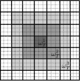
We refer to Figure 1 for an illustration.

Refer to caption
Figure 1: Example of a one layer patch ωT1subscriptsuperscript𝜔1𝑇\omega^{1}_{T}, two layer patch ωT2subscriptsuperscript𝜔2𝑇\omega^{2}_{T}, and a three layer patch ωT3subscriptsuperscript𝜔3𝑇\omega^{3}_{T}, on a quadrilateral mesh.

We introduce a new discretization parameter L>0𝐿0L>0\in\mathbb{N} and define localized corrector functions ϕT,jL𝒱f(ωTL):={v𝒱fv|ΩωTL=0}subscriptsuperscriptitalic-ϕ𝐿𝑇𝑗superscript𝒱fsubscriptsuperscript𝜔𝐿𝑇assignconditional-set𝑣superscript𝒱fevaluated-at𝑣Ωsubscriptsuperscript𝜔𝐿𝑇0\phi^{L}_{T,j}\in\mathcal{V}^{\operatorname*{f}}(\omega^{L}_{T}):=\{v\in\mathcal{V}^{\operatorname*{f}}\mid v|_{\Omega\setminus\omega^{L}_{T}}=0\} by

ah(ϕT,jL,w)=ah(λT,j,w)for all w𝒱f(ωTL).formulae-sequencesubscript𝑎subscriptsuperscriptitalic-ϕ𝐿𝑇𝑗𝑤subscript𝑎subscript𝜆𝑇𝑗𝑤for all 𝑤superscript𝒱fsubscriptsuperscript𝜔𝐿𝑇a_{h}(\phi^{L}_{T,j},w)=a_{h}(\lambda_{T,j},w)\quad\text{for all }w\in\mathcal{V}^{\operatorname*{f}}(\omega^{L}_{T}). (3.3)

Further, we define the multiscale approximation space

𝒱Hms,L=span{λT,jϕT,jL|T𝒯H,j=1,,r},subscriptsuperscript𝒱𝑚𝑠𝐿𝐻spanconditional-setsubscript𝜆𝑇𝑗subscriptsuperscriptitalic-ϕ𝐿𝑇𝑗formulae-sequence𝑇subscript𝒯𝐻𝑗1𝑟\mathcal{V}^{ms,L}_{H}=\text{span}\{\lambda_{T,j}-\phi^{L}_{T,j}\;|\;T\in\mathcal{T}_{H},\;j=1,\ldots,r\},

The dG multiscale method seeks uHms,L𝒱Hms,Lsubscriptsuperscript𝑢𝑚𝑠𝐿𝐻subscriptsuperscript𝒱𝑚𝑠𝐿𝐻u^{ms,L}_{H}\in\mathcal{V}^{ms,L}_{H} such that

ah(uHms,L,v)=F(v)for all v𝒱Hms,L.formulae-sequencesubscript𝑎subscriptsuperscript𝑢𝑚𝑠𝐿𝐻𝑣𝐹𝑣for all 𝑣subscriptsuperscript𝒱𝑚𝑠𝐿𝐻a_{h}(u^{ms,L}_{H},v)=F(v)\quad\text{for all }v\in\mathcal{V}^{ms,L}_{H}. (3.4)

Since 𝒱Hms,L𝒱hsubscriptsuperscript𝒱𝑚𝑠𝐿𝐻subscript𝒱\mathcal{V}^{ms,L}_{H}\subset\mathcal{V}_{h}, this method is a Galerkin method in the Hilbert space 𝒱hsubscript𝒱\mathcal{V}_{h} (with scalar product ahsubscript𝑎a_{h}) and, hence, inherits well-posedness from the reference discretization (2.4).

Moreover, the proposed basis {λT,jϕT,jL|T𝒯H,j=1,,r}conditional-setsubscript𝜆𝑇𝑗subscriptsuperscriptitalic-ϕ𝐿𝑇𝑗formulae-sequence𝑇subscript𝒯𝐻𝑗1𝑟\{\lambda_{T,j}-\phi^{L}_{T,j}\;|\;T\in\mathcal{T}_{H},\;j=1,\ldots,r\} is stable with respect to the fine scale parameter hh, as we shall see in Lemma 7 below.

3.3 Compressed discontinuous Galerkin multiscale method

The basis functions in the above multiscale method have enlarged supports (element patches) when compared with standard dG methods (elements). We can decompose the corrector functions into its element contributions

ϕT,jL=T𝒯H:TωTLϕT,jLχT,subscriptsuperscriptitalic-ϕ𝐿𝑇𝑗subscript:superscript𝑇subscript𝒯𝐻superscript𝑇superscriptsubscript𝜔𝑇𝐿subscriptsuperscriptitalic-ϕ𝐿𝑇𝑗subscript𝜒superscript𝑇\phi^{L}_{T,j}=\sum_{T^{\prime}\in\mathcal{T}_{H}:T^{\prime}\subset\omega_{T}^{L}}\phi^{L}_{T,j}\chi_{T^{\prime}},

where χTsubscript𝜒superscript𝑇\chi_{T^{\prime}} is the indicator function of the element T𝒯Hsuperscript𝑇subscript𝒯𝐻T^{\prime}\in\mathcal{T}_{H}.

This motivates the coarse approximation space

𝒲Hms,L=subscriptsuperscript𝒲𝑚𝑠𝐿𝐻absent\displaystyle\mathcal{W}^{ms,L}_{H}= span({λT,j|T𝒯H,j=1,,r}\displaystyle\text{span}\bigl{(}\{\lambda_{T,j}\;|T\in\mathcal{T}_{H},\;j=1,\ldots,r\}
{ϕT,jLχT|T,T𝒯H,TωTL,j=1,,r},conditional-setsubscriptsuperscriptitalic-ϕ𝐿𝑇𝑗subscript𝜒superscript𝑇formulae-sequence𝑇superscript𝑇subscript𝒯𝐻formulae-sequencesuperscript𝑇superscriptsubscript𝜔𝑇𝐿𝑗1𝑟\displaystyle\cup\{\phi^{L}_{T,j}\chi_{T^{\prime}}\;|T,T^{\prime}\in\mathcal{T}_{H},\;T^{\prime}\subset\omega_{T}^{L},\;j=1,\ldots,r\},

This space offers the advantage of a known basis with element-wise support which leads to improved (localized) connectivity in the corresponding stiffness matrix. This is at the expense of a slight increase in the dimension of the space

dim(𝒲Hms,L)Lddim(𝒱Hms,L).dimsubscriptsuperscript𝒲𝑚𝑠𝐿𝐻superscript𝐿𝑑dimsubscriptsuperscript𝒱𝑚𝑠𝐿𝐻\operatorname*{dim}(\mathcal{W}^{ms,L}_{H})\approx L^{d}\operatorname*{dim}(\mathcal{V}^{ms,L}_{H}).

The corresponding localized dG multiscale method seeks wHms,L𝒲Hms,Lsubscriptsuperscript𝑤𝑚𝑠𝐿𝐻subscriptsuperscript𝒲𝑚𝑠𝐿𝐻w^{ms,L}_{H}\in\mathcal{W}^{ms,L}_{H} such that

ah(wHms,L,v)=F(v)for all v𝒲Hms,L.formulae-sequencesubscript𝑎subscriptsuperscript𝑤𝑚𝑠𝐿𝐻𝑣𝐹𝑣for all 𝑣subscriptsuperscript𝒲𝑚𝑠𝐿𝐻a_{h}(w^{ms,L}_{H},v)=F(v)\quad\text{for all }v\in\mathcal{W}^{ms,L}_{H}. (3.5)

Since 𝒱Hms,L𝒲Hms,L𝒱hsubscriptsuperscript𝒱𝑚𝑠𝐿𝐻subscriptsuperscript𝒲𝑚𝑠𝐿𝐻subscript𝒱\mathcal{V}^{ms,L}_{H}\subset\mathcal{W}^{ms,L}_{H}\subset\mathcal{V}_{h}, Galerkin orthogonality yields

|uhwHms,L|h|uhuHms,L|h,subscriptnormsubscript𝑢subscriptsuperscript𝑤𝑚𝑠𝐿𝐻subscriptnormsubscript𝑢subscriptsuperscript𝑢𝑚𝑠𝐿𝐻|||u_{h}-w^{ms,L}_{H}|||_{h}\leq|||u_{h}-u^{ms,L}_{H}|||_{h}, (3.6)

i.e., the new localized version (3.5) is never worse than the previous multiscale approximation in terms of accuracy. However, it may lead to very ill-conditioned element stiffness matrices (cf. Lemma 10 which shows that ϕT,jLξTsubscriptsuperscriptitalic-ϕ𝐿𝑇𝑗subscript𝜉superscript𝑇\phi^{L}_{T,j}\xi_{T^{\prime}} may be very small if the distance between T𝑇T and Tsuperscript𝑇T^{\prime} relative to their sizes is large).

To circumvent ill-conditioning, one may choose a reduced local approximation space on the basis of a singular value decomposition. Since the dimension of the local approximation space is small (at most proportional to Ldsuperscript𝐿𝑑L^{d}), the cost for this additional preprocessing step is comparable with the cost for the solution of the local problems for the corrector functions.

To determine an acceptable level of truncation of the localized basis functions, we can use the the a posteriori error estimator contribution of the local problem from [8], which is an estimation of the local fine scale error. This procedure may additionally lead to large reduction of the dimension of the local approximation spaces.

4 Error analysis

We present an a priori error analysis for the proposed multiscale method (3.4). In view of (3.6), this analysis applies immediately to the modified versions presented in Section 3.3. The error analysis will be split into a number of steps. First, in Section 4.1, we present some properties of the coarse scale projection operator ΠHsubscriptΠ𝐻\Pi_{H}. In Section 4.2, an error bound for dG multiscale method uHmssubscriptsuperscript𝑢𝑚𝑠𝐻u^{ms}_{H} from (3.2) (Theorem 8) is shown, whereby the corrected basis functions are solved globally. Results for the decay of the localized corrected basis function (Lemma 10 and Lemma 11) are shown, along with an error bound for the dG multiscale method uHms,Lsubscriptsuperscript𝑢𝑚𝑠𝐿𝐻u^{ms,L}_{H} from (3.4) (Theorem 12) ,where the corrected basis functions are solved locally on element patches. Finally, in Section 4.3, we show an error bound given a quantity of interest (Theorem 14), leading to an error bound in L2superscript𝐿2L^{2}-norm (Corollary 15).

We shall make use of the following (semi)norms. The jump-seminorm and energy norms, associated with the coarse space 𝒱Hsubscript𝒱𝐻\mathcal{V}_{H}, are defined by

||H2\displaystyle|\bullet|_{H}^{2} :=eH(Ω)H(ΓD)σHe[]L2(e)2,assignabsentsubscript𝑒subscript𝐻Ωsubscript𝐻subscriptΓ𝐷𝜎subscript𝐻𝑒superscriptsubscriptnormdelimited-[]superscript𝐿2𝑒2\displaystyle:=\sum_{e\in\mathcal{E}_{H}(\Omega)\cup\mathcal{E}_{H}(\Gamma_{D})}\frac{\sigma}{H_{e}}\|[\bullet]\|_{L^{2}(e)}^{2},
||||||H\displaystyle|||\bullet|||_{H} :=(A1/2HL2(Ω)2+||H2)1/2,\displaystyle:=(\|A^{1/2}\nabla_{H}\bullet\|_{L^{2}(\Omega)}^{2}+|\bullet|_{H}^{2})^{1/2},

respectively, along with a localized version of the local jump and energy norms (2.2) and (2.3) on a patch ωΩ𝜔Ω\omega\subseteq\Omega, where ω𝜔\omega is aligned with the mesh 𝒯hsubscript𝒯\mathcal{T}_{h}, given by

||h,ω2\displaystyle|\bullet|_{h,\omega}^{2} :=e(Ω)(ΓD):eω¯0σhe[]L2(e)2,assignabsentsubscript:𝑒ΩsubscriptΓ𝐷absent𝑒¯𝜔0𝜎subscript𝑒superscriptsubscriptnormdelimited-[]superscript𝐿2𝑒2\displaystyle:=\sum_{\begin{subarray}{c}e\in\mathcal{E}(\Omega)\cup\mathcal{E}(\Gamma_{D}):\\ e\cap\bar{\omega}\neq 0\end{subarray}}\frac{\sigma}{h_{e}}\|[\bullet]\|_{L^{2}(e)}^{2},
||||||h,ω\displaystyle|||\bullet|||_{h,\omega} :=(A1/2hL2(ω)2+||h,ω2)1/2.\displaystyle:=(\|A^{1/2}\nabla_{h}\bullet\|_{L^{2}(\omega)}^{2}+|\bullet|_{h,\omega}^{2})^{1/2}.

The shape-regularity assumptions hThesubscript𝑇subscript𝑒h_{T}\approx h_{e} for all eT:T𝒯h:𝑒𝑇𝑇subscript𝒯e\in\partial T:T\in\mathcal{T}_{h} and HTHesubscript𝐻𝑇subscript𝐻𝑒H_{T}\approx H_{e} for all TT:T𝒯H:𝑇𝑇𝑇subscript𝒯𝐻T\in\partial T:T\in\mathcal{T}_{H} will also be used.

4.1 Properties of the coarse scale projection operator ΠHsubscriptΠ𝐻\Pi_{H}

The following lemma gives stability and approximation properties of the operator ΠHsubscriptΠ𝐻\Pi_{H}.

Lemma 4.

For any v𝒱h𝑣subscript𝒱v\in\mathcal{V}_{h}, the estimate

H1vΠHvL2(T)α1/2|v|h,T,less-than-or-similar-tosuperscript𝐻1subscriptnorm𝑣subscriptΠ𝐻𝑣superscript𝐿2𝑇superscript𝛼12subscriptnorm𝑣𝑇\displaystyle H^{-1}\|v-\Pi_{H}v\|_{L^{2}(T)}\lesssim\alpha^{-1/2}|||v|||_{h,T},

is satisfied for all T𝒯H𝑇subscript𝒯𝐻T\in\mathcal{T}_{H}. Moreover, it holds

β1/2|ΠHv|H+H1(vΠHv)L2(Ω)α1/2|v|h.less-than-or-similar-tosuperscript𝛽12subscriptnormsubscriptΠ𝐻𝑣𝐻subscriptnormsuperscript𝐻1𝑣subscriptΠ𝐻𝑣superscript𝐿2Ωsuperscript𝛼12subscriptnorm𝑣\displaystyle\beta^{-1/2}|||\Pi_{H}v|||_{H}+\|H^{-1}(v-\Pi_{H}v)\|_{L^{2}(\Omega)}\lesssim\alpha^{-1/2}|||v|||_{h}.
Proof.

Theorem 2.2 in [12], implies that for each v𝒱h𝑣subscript𝒱v\in\mathcal{V}_{h}, there exists a bounded linear operator hc:𝒱h𝒱hH1(Ω):subscriptsuperscriptcsubscript𝒱subscript𝒱superscript𝐻1Ω\mathcal{I}^{\operatorname*{c}}_{h}:\mathcal{V}_{h}\rightarrow\mathcal{V}_{h}\cap H^{1}(\Omega) such that

β1/2A1/2H(vhcv)L2(Ω)+h1(vhcv)L2(Ω)α1/2|v|h.less-than-or-similar-tosuperscript𝛽12subscriptnormsuperscript𝐴12subscript𝐻𝑣subscriptsuperscriptc𝑣superscript𝐿2Ωsubscriptnormsuperscript1𝑣subscriptsuperscriptc𝑣superscript𝐿2Ωsuperscript𝛼12subscript𝑣\beta^{-1/2}\|A^{1/2}\nabla_{H}(v-\mathcal{I}^{\operatorname*{c}}_{h}v)\|_{L^{2}(\Omega)}+\|h^{-1}(v-\mathcal{I}^{\operatorname*{c}}_{h}v)\|_{L^{2}(\Omega)}\lesssim\alpha^{-1/2}|v|_{h}. (4.1)

Split v=vc+vd𝒱h𝑣superscript𝑣csuperscript𝑣dsubscript𝒱v=v^{\operatorname*{c}}+v^{\operatorname*{d}}\in\mathcal{V}_{h} into a conforming, vc=hcvsuperscript𝑣csubscriptsuperscriptc𝑣v^{\operatorname*{c}}=\mathcal{I}^{\operatorname*{c}}_{h}v, and non-conforming, vd=vhcvsuperscript𝑣d𝑣subscriptsuperscriptc𝑣v^{\operatorname*{d}}=v-\mathcal{I}^{\operatorname*{c}}_{h}v, part. We obtain

H1vΠHvL2(T)superscript𝐻1subscriptnorm𝑣subscriptΠ𝐻𝑣superscript𝐿2𝑇\displaystyle H^{-1}\|v-\Pi_{H}v\|_{L^{2}(T)} H1(vcΠHvcL2(T)+vdΠHvdL2(T))absentsuperscript𝐻1subscriptnormsuperscript𝑣csubscriptΠ𝐻superscript𝑣csuperscript𝐿2𝑇subscriptnormsuperscript𝑣dsubscriptΠ𝐻superscript𝑣dsuperscript𝐿2𝑇\displaystyle\leq H^{-1}(\|v^{\operatorname*{c}}-\Pi_{H}v^{\operatorname*{c}}\|_{L^{2}(T)}+\|v^{\operatorname*{d}}-\Pi_{H}v^{\operatorname*{d}}\|_{L^{2}(T)}) (4.2)
hv+h(vvc)L2(T)+H1vdL2(T))\displaystyle\lesssim\|\nabla_{h}v\|+\|\nabla_{h}(v-v^{\operatorname*{c}})\|_{L^{2}(T)}+H^{-1}\|v^{\operatorname*{d}}\|_{L^{2}(T)})
α1/2|v|h,Tless-than-or-similar-toabsentsuperscript𝛼12subscriptnorm𝑣𝑇\displaystyle\lesssim\alpha^{-1/2}|||v|||_{h,T}

using the triangle inequality, stability of the L2superscript𝐿2L^{2}-projection, and (4.1). Also,

|ΠHv|H2=superscriptsubscriptnormsubscriptΠ𝐻𝑣𝐻2absent\displaystyle|||\Pi_{H}v|||_{H}^{2}= T𝒯HA(ΠHvΠ0(𝒯H)v)L2(T)2+eΓσH[vcΠHv]L2(e)2subscript𝑇subscript𝒯𝐻subscriptsuperscriptnorm𝐴subscriptΠ𝐻𝑣subscriptΠ0subscript𝒯𝐻𝑣2superscript𝐿2𝑇subscript𝑒Γ𝜎𝐻subscriptsuperscriptnormdelimited-[]subscript𝑣𝑐subscriptΠ𝐻𝑣2superscript𝐿2𝑒\displaystyle\sum_{T\in\mathcal{T}_{H}}\|\sqrt{A}\nabla(\Pi_{H}v-\Pi_{0}(\mathcal{T}_{H})v)\|^{2}_{L^{2}(T)}+\sum_{e\in\Gamma}\frac{\sigma}{H}\|[v_{c}-\Pi_{H}v]\|^{2}_{L^{2}(e)}
less-than-or-similar-to\displaystyle\lesssim T𝒯Hβ(1H2vΠ0(𝒯H)vL2(T)2+1H2vcΠHvL2(T)2)subscript𝑇subscript𝒯𝐻𝛽1superscript𝐻2subscriptsuperscriptnorm𝑣subscriptΠ0subscript𝒯𝐻𝑣2superscript𝐿2𝑇1superscript𝐻2subscriptsuperscriptnormsubscript𝑣𝑐subscriptΠ𝐻𝑣2superscript𝐿2𝑇\displaystyle\sum_{T\in\mathcal{T}_{H}}\beta\left(\frac{1}{H^{2}}\|v-\Pi_{0}(\mathcal{T}_{H})v\|^{2}_{L^{2}(T)}+\frac{1}{H^{2}}\|v_{c}-\Pi_{H}v\|^{2}_{L^{2}(T)}\right)
less-than-or-similar-to\displaystyle\lesssim Cβ/α2|v|h2,superscriptsubscript𝐶𝛽𝛼2superscriptsubscriptnorm𝑣2\displaystyle C_{\beta/\alpha}^{2}|||v|||_{h}^{2},

using the triangle inequality, (4.1), and (4.2) which concludes the proof. ∎

The operator ΠHsubscriptΠ𝐻\Pi_{H} is surjective. The next lemma shows that, given some vH𝒱Hsubscript𝑣𝐻subscript𝒱𝐻v_{H}\in\mathcal{V}_{H} in the image of ΠHsubscriptΠ𝐻\Pi_{H} there exists a H1superscript𝐻1H^{1}-conforming pre-image vΠH1vH𝒱h𝑣superscriptsubscriptΠ𝐻1subscript𝑣𝐻subscript𝒱v\in\Pi_{H}^{-1}v_{H}\subset\mathcal{V}_{h} with comparable support.

Lemma 5.

For each vH𝒱Hsubscript𝑣𝐻subscript𝒱𝐻v_{H}\in\mathcal{V}_{H}, there exists a v𝒱hH1(Ω)𝑣subscript𝒱superscript𝐻1Ωv\in\mathcal{V}_{h}\cap H^{1}(\Omega) such that ΠHv=vHsubscriptΠ𝐻𝑣subscript𝑣𝐻\Pi_{H}v=v_{H}, |v|hCβ/α|vH|Hless-than-or-similar-tosubscriptnorm𝑣subscript𝐶𝛽𝛼subscriptnormsubscript𝑣𝐻𝐻|||v|||_{h}\lesssim C_{\beta/\alpha}|||v_{H}|||_{H}, and supp(v)supp(vH)supp𝑣suppsubscript𝑣𝐻\text{supp}(v)\subseteq\text{supp}(v_{H}).

Proof.

Using (4.1) but on space 𝒱Hsubscript𝒱𝐻\mathcal{V}_{H} gives, for each v𝒱H𝑣subscript𝒱𝐻v\in\mathcal{V}_{H}, there exists a bounded linear operator Hc:𝒱H𝒱HH1(Ω):subscriptsuperscriptc𝐻subscript𝒱𝐻subscript𝒱𝐻superscript𝐻1Ω\mathcal{I}^{\operatorname*{c}}_{H}:\mathcal{V}_{H}\rightarrow\mathcal{V}_{H}\cap H^{1}(\Omega) such that

β1/2A1/2H(vHcv)L2(Ω)+H1(vHcv)L2(Ω)α1/2|v|H.less-than-or-similar-tosuperscript𝛽12subscriptnormsuperscript𝐴12subscript𝐻𝑣subscriptsuperscriptc𝐻𝑣superscript𝐿2Ωsubscriptnormsuperscript𝐻1𝑣subscriptsuperscriptc𝐻𝑣superscript𝐿2Ωsuperscript𝛼12subscript𝑣𝐻\beta^{-1/2}\|A^{1/2}\nabla_{H}(v-\mathcal{I}^{\operatorname*{c}}_{H}v)\|_{L^{2}(\Omega)}+\|H^{-1}(v-\mathcal{I}^{\operatorname*{c}}_{H}v)\|_{L^{2}(\Omega)}\lesssim\alpha^{-1/2}|v|_{H}. (4.3)

We define

v:=HcvH+T𝒯H,j=1,,r(vH(xj)HcvH(xj))θT,j,assign𝑣subscriptsuperscriptc𝐻subscript𝑣𝐻subscriptformulae-sequence𝑇subscript𝒯𝐻𝑗1𝑟subscript𝑣𝐻subscript𝑥𝑗subscriptsuperscriptc𝐻subscript𝑣𝐻subscript𝑥𝑗subscript𝜃𝑇𝑗v:=\mathcal{I}^{\operatorname*{c}}_{H}v_{H}+\sum_{T\in\mathcal{T}_{H},\;j=1,\ldots,r}\left(v_{H}(x_{j})-\mathcal{I}^{\operatorname*{c}}_{H}v_{H}(x_{j})\right)\theta_{T,j},

where θT,j𝒱hH01(T)subscript𝜃𝑇𝑗subscript𝒱subscriptsuperscript𝐻10𝑇\theta_{T,j}\in\mathcal{V}_{h}\cap H^{1}_{0}(T) are bubble functions, supported on each element T𝑇T, with ΠHθT,j=λT,jsubscriptΠ𝐻subscript𝜃𝑇𝑗subscript𝜆𝑇𝑗\Pi_{H}\theta_{T,j}=\lambda_{T,j} and |θT,j|hβ(T)Hd2less-than-or-similar-tosubscriptnormsubscript𝜃𝑇𝑗𝛽𝑇superscript𝐻𝑑2|||\theta_{T,j}|||_{h}\lesssim\beta(T)H^{d-2}. Observe that supp(v)supp(vH)supp𝑣suppsubscript𝑣𝐻\text{supp}(v)\subseteq\text{supp}(v_{H}). The interpolation property follows from

ΠHvsubscriptΠ𝐻𝑣\displaystyle\Pi_{H}v =HcvH+ΠHT𝒯H,j=1,,r(vH(xj)HcvH(xj))θj,absentsubscriptsuperscriptc𝐻subscript𝑣𝐻subscriptΠ𝐻subscriptformulae-sequence𝑇subscript𝒯𝐻𝑗1𝑟subscript𝑣𝐻subscript𝑥𝑗subscriptsuperscriptc𝐻subscript𝑣𝐻subscript𝑥𝑗subscript𝜃𝑗\displaystyle=\mathcal{I}^{\operatorname*{c}}_{H}v_{H}+\Pi_{H}\sum_{T\in\mathcal{T}_{H},\;j=1,\ldots,r}\left(v_{H}(x_{j})-\mathcal{I}^{\operatorname*{c}}_{H}v_{H}(x_{j})\right)\theta_{j},
=HcvH+vHHcvH=vH.absentsubscriptsuperscriptc𝐻subscript𝑣𝐻subscript𝑣𝐻subscriptsuperscriptc𝐻subscript𝑣𝐻subscript𝑣𝐻\displaystyle=\mathcal{I}^{\operatorname*{c}}_{H}v_{H}+v_{H}-\mathcal{I}^{\operatorname*{c}}_{H}v_{H}=v_{H}.

To prove stability, we estimate |v|hsubscriptnorm𝑣|||v|||_{h} as follows:

|v|h2superscriptsubscriptnorm𝑣2\displaystyle|||v|||_{h}^{2} A1/2HcvHL2(Ω)2+T𝒯H,j=1,,r|vH(xj)HcvH(xj)|2|θj|h2absentsubscriptsuperscriptnormsuperscript𝐴12subscriptsuperscriptc𝐻subscript𝑣𝐻2superscript𝐿2Ωsubscriptformulae-sequence𝑇subscript𝒯𝐻𝑗1𝑟superscriptsubscript𝑣𝐻subscript𝑥𝑗subscriptsuperscriptc𝐻subscript𝑣𝐻subscript𝑥𝑗2superscriptsubscriptnormsubscript𝜃𝑗2\displaystyle\leq\|A^{1/2}\nabla\mathcal{I}^{\operatorname*{c}}_{H}v_{H}\|^{2}_{L^{2}(\Omega)}+\sum_{T\in\mathcal{T}_{H},\;j=1,\ldots,r}\left|v_{H}(x_{j})-\mathcal{I}^{\operatorname*{c}}_{H}v_{H}(x_{j})\right|^{2}|||\theta_{j}|||_{h}^{2}
A1/2HHcvHL2(Ω)2+βH1(vHHcvH)L2(Ω)2less-than-or-similar-toabsentsubscriptsuperscriptnormsuperscript𝐴12subscript𝐻subscriptsuperscriptc𝐻subscript𝑣𝐻2superscript𝐿2Ω𝛽subscriptsuperscriptnormsuperscript𝐻1subscript𝑣𝐻subscriptsuperscriptc𝐻subscript𝑣𝐻2superscript𝐿2Ω\displaystyle\lesssim\|A^{1/2}\nabla_{H}\mathcal{I}^{\operatorname*{c}}_{H}v_{H}\|^{2}_{L^{2}(\Omega)}+\beta\|H^{-1}(v_{H}-\mathcal{I}^{\operatorname*{c}}_{H}v_{H})\|^{2}_{L^{2}(\Omega)}
Cβ/α2|vH|H2less-than-or-similar-toabsentsuperscriptsubscript𝐶𝛽𝛼2superscriptsubscriptnormsubscript𝑣𝐻𝐻2\displaystyle\lesssim C_{\beta/\alpha}^{2}|||v_{H}|||_{H}^{2}

using the inverse estimate vL(T)Hd/2vL2(T)subscriptnorm𝑣superscript𝐿𝑇superscript𝐻𝑑2subscriptnorm𝑣superscript𝐿2𝑇\|v\|_{L^{\infty}(T)}\leq H^{-d/2}\|v\|_{L^{2}(T)} for all v𝒱H𝑣subscript𝒱𝐻v\in\mathcal{V}_{H}, and the estimate (4.3). ∎

Remark 6.

Note that θT,j𝒱hH01(T)subscript𝜃𝑇𝑗subscript𝒱subscriptsuperscript𝐻10𝑇\theta_{T,j}\in\mathcal{V}_{h}\cap H^{1}_{0}(T) for all T𝒯H𝑇subscript𝒯𝐻T\in\mathcal{T}_{H} (fulfilling the conditions in Lemma 5) can be constructed using two (or more) refinements of the coarse scale parameter H𝐻H. We can let θT,j𝒱hH01(T)subscript𝜃𝑇𝑗subscript𝒱superscriptsubscriptsuperscript𝐻10𝑇\theta_{T,j}\in\mathcal{V}_{h^{\prime}}\cap H^{1}_{0}(T) where 𝒱h𝒱hsubscript𝒱superscriptsubscript𝒱\mathcal{V}_{h^{\prime}}\subset\mathcal{V}_{h} and hh22Hsuperscriptsuperscript22𝐻h\leq h^{\prime}\leq 2^{-2}H. This does not put a big restriction on hh since the mesh 𝒯hsubscript𝒯\mathcal{T}_{h} is assumed to be sufficiently fine to resolve the variation in the coefficient A𝐴A, while the parameter H𝐻H does not need to resolve A𝐴A.

The following lemma says that the corrected basis is stable with respect to the fine scale parameter hh in the energy norm (2.3), this is not a trivial result since the basis function {λT,j|T𝒯H,j=1,,r}conditional-setsubscript𝜆𝑇𝑗formulae-sequence𝑇subscript𝒯𝐻𝑗1𝑟\{\lambda_{T,j}|T\in\mathcal{T}_{H},\;j=1,\ldots,r\} are discontinuous.

Lemma 7 (Stability of the corrected basis functions).

For all, T𝒯H,j=1,,rformulae-sequence𝑇subscript𝒯𝐻𝑗1𝑟T\in\mathcal{T}_{H},\;j=1,\ldots,r and L>0𝐿0L>0\in\mathbb{N}, the estimate

|λT,jϕT,jL|hCβ/α|λT,j|H,less-than-or-similar-tosubscriptnormsubscript𝜆𝑇𝑗subscriptsuperscriptitalic-ϕ𝐿𝑇𝑗subscript𝐶𝛽𝛼subscriptnormsubscript𝜆𝑇𝑗𝐻|||\lambda_{T,j}-\phi^{L}_{T,j}|||_{h}\lesssim C_{\beta/\alpha}|||\lambda_{T,j}|||_{H},

is satisfied, independently of the fine scale parameter hh.

Proof.

For any T𝒯H,j=1,,rformulae-sequence𝑇subscript𝒯𝐻𝑗1𝑟T\in\mathcal{T}_{H},\;j=1,\ldots,r, by Lemma 5 there exists a b𝑏b such that v=λT,jb𝒱hf(ωTL)𝑣subscript𝜆𝑇𝑗𝑏subscriptsuperscript𝒱𝑓superscriptsubscript𝜔𝑇𝐿v=\lambda_{T,j}-b\in\mathcal{V}^{f}_{h}(\omega_{T}^{L}), and |b|hCβ/α|λT,j|Hless-than-or-similar-tosubscriptnorm𝑏subscript𝐶𝛽𝛼subscriptnormsubscript𝜆𝑇𝑗𝐻|||b|||_{h}\lesssim C_{\beta/\alpha}|||\lambda_{T,j}|||_{H}. We have

|λT,jϕT,jL|h2superscriptsubscriptnormsubscript𝜆𝑇𝑗subscriptsuperscriptitalic-ϕ𝐿𝑇𝑗2\displaystyle|||\lambda_{T,j}-\phi^{L}_{T,j}|||_{h}^{2} ah(λT,jϕT,jL,λT,jϕT,jL)=ah(λT,jϕT,jL,λT,jv),less-than-or-similar-toabsentsubscript𝑎subscript𝜆𝑇𝑗subscriptsuperscriptitalic-ϕ𝐿𝑇𝑗subscript𝜆𝑇𝑗subscriptsuperscriptitalic-ϕ𝐿𝑇𝑗subscript𝑎subscript𝜆𝑇𝑗subscriptsuperscriptitalic-ϕ𝐿𝑇𝑗subscript𝜆𝑇𝑗𝑣\displaystyle\lesssim a_{h}(\lambda_{T,j}-\phi^{L}_{T,j},\lambda_{T,j}-\phi^{L}_{T,j})=a_{h}(\lambda_{T,j}-\phi^{L}_{T,j},\lambda_{T,j}-v),
ah(λT,jϕT,jL,b)Cβ/α|λT,jϕT,jL|h|λT,j|H,less-than-or-similar-toabsentsubscript𝑎subscript𝜆𝑇𝑗subscriptsuperscriptitalic-ϕ𝐿𝑇𝑗𝑏less-than-or-similar-tosubscript𝐶𝛽𝛼subscriptnormsubscript𝜆𝑇𝑗subscriptsuperscriptitalic-ϕ𝐿𝑇𝑗subscriptnormsubscript𝜆𝑇𝑗𝐻\displaystyle\lesssim a_{h}(\lambda_{T,j}-\phi^{L}_{T,j},b)\lesssim C_{\beta/\alpha}|||\lambda_{T,j}-\phi^{L}_{T,j}|||_{h}|||\lambda_{T,j}|||_{H},

which concludes the proof. ∎

4.2 A priori estimates

The following theorem gives an error bound for the idealized dG multiscale method, whereby the correctors for the basis are solved globally.

Theorem 8.

Let uh𝒱hsubscript𝑢subscript𝒱u_{h}\in\mathcal{V}_{h} solve (2.4) and uHms𝒱Hmssubscriptsuperscript𝑢𝑚𝑠𝐻subscriptsuperscript𝒱𝑚𝑠𝐻u^{ms}_{H}\in\mathcal{V}^{ms}_{H} solve (3.4), then the estimate

|uhuHms|hC1α1/2H(fΠHf)L2(Ω),subscriptnormsubscript𝑢subscriptsuperscript𝑢𝑚𝑠𝐻subscript𝐶1superscript𝛼12subscriptnorm𝐻𝑓subscriptΠ𝐻𝑓superscript𝐿2Ω|||u_{h}-u^{ms}_{H}|||_{h}\leq C_{1}\alpha^{-1/2}||H(f-\Pi_{H}f)||_{L^{2}(\Omega)},

is satisfied, where C1subscript𝐶1C_{1} neither depends on the mesh (hh or H𝐻H) size nor the diffusion matrix A𝐴A.

Proof.

Let e:=uhuHms=uf𝒱fassign𝑒subscript𝑢subscriptsuperscript𝑢𝑚𝑠𝐻subscript𝑢𝑓superscript𝒱fe:=u_{h}-u^{ms}_{H}=u_{f}\in\mathcal{V}^{\operatorname*{f}}, then

|e|h2superscriptsubscriptnorm𝑒2\displaystyle|||e|||_{h}^{2} ah(e,e)=(f,e)L2(Ω)=(fΠHf,eΠHe)L2(Ω)less-than-or-similar-toabsentsubscript𝑎𝑒𝑒subscript𝑓𝑒superscript𝐿2Ωsubscript𝑓subscriptΠ𝐻𝑓𝑒subscriptΠ𝐻𝑒superscript𝐿2Ω\displaystyle\lesssim a_{h}(e,e)=(f,e)_{L^{2}(\Omega)}=(f-\Pi_{H}f,e-\Pi_{H}e)_{L^{2}(\Omega)}
H(fΠHf)L2(Ω)H1(eΠHe)L2(Ω)2absentsubscriptnorm𝐻𝑓subscriptΠ𝐻𝑓superscript𝐿2Ωsubscriptsuperscriptnormsuperscript𝐻1𝑒subscriptΠ𝐻𝑒2superscript𝐿2Ω\displaystyle\leq||H(f-\Pi_{H}f)||_{L^{2}(\Omega)}||H^{-1}(e-\Pi_{H}e)||^{2}_{L^{2}(\Omega)}
1αH(fΠHf)L2(T)|e|h,less-than-or-similar-toabsent1𝛼subscriptnorm𝐻𝑓subscriptΠ𝐻𝑓superscript𝐿2𝑇subscriptnorm𝑒\displaystyle\lesssim\frac{1}{\sqrt{\alpha}}||H(f-\Pi_{H}f)||_{L^{2}(T)}|||e|||_{h},

using Lemma 2, Lemma 1, Cauchy-Schwarz inequality, and Lemma 4, respectively. ∎

Definition 9.

The cut off functions ζTd,DP0(𝒯h)superscriptsubscript𝜁𝑇𝑑𝐷subscript𝑃0subscript𝒯\zeta_{T}^{d,D}\in P_{0}(\mathcal{T}_{h}) are defined by the conditions

ζTd,D|ωTdevaluated-atsuperscriptsubscript𝜁𝑇𝑑𝐷superscriptsubscript𝜔𝑇𝑑\displaystyle\zeta_{T}^{d,D}|_{\omega_{T}^{d}} =1,absent1\displaystyle=1,
ζTd,D|ΩωTDevaluated-atsuperscriptsubscript𝜁𝑇𝑑𝐷Ωsubscriptsuperscript𝜔𝐷𝑇\displaystyle\zeta_{T}^{d,D}|_{\Omega\setminus\omega^{D}_{T}} =0,absent0\displaystyle=0,
[ζTd,D]L(T)subscriptnormdelimited-[]superscriptsubscript𝜁𝑇𝑑𝐷superscript𝐿𝑇\displaystyle\|[\zeta_{T}^{d,D}]\|_{L^{\infty}(T)} hT(Dd)HTfor all T𝒯H,formulae-sequenceless-than-or-similar-toabsentsubscript𝑇𝐷𝑑subscript𝐻𝑇for all 𝑇subscript𝒯𝐻\displaystyle\lesssim\frac{h_{T}}{(D-d)H_{T}}\quad\text{for all }T\in\mathcal{T}_{H},

and that ζTd,Dsuperscriptsubscript𝜁𝑇𝑑𝐷\zeta_{T}^{d,D} is constant on the boundary (ωTDωTd)subscriptsuperscript𝜔𝐷𝑇subscriptsuperscript𝜔𝑑𝑇\partial(\omega^{D}_{T}\setminus\omega^{d}_{T}).

The next lemma shows the exponential decay in the corrected basis, which is a key result in the analysis.

Lemma 10.

For all T𝒯H,j=1,,rformulae-sequence𝑇subscript𝒯𝐻𝑗1𝑟T\in\mathcal{T}_{H},\;j=1,\ldots,r, the estimate

|(λjϕT,j)(λjϕT,jL)|h=|ϕT,jϕT,jL|hC3γL|ϕT,jλ|h,subscriptnormsubscript𝜆𝑗subscriptitalic-ϕ𝑇𝑗subscript𝜆𝑗subscriptsuperscriptitalic-ϕ𝐿𝑇𝑗subscriptnormsubscriptitalic-ϕ𝑇𝑗subscriptsuperscriptitalic-ϕ𝐿𝑇𝑗subscript𝐶3superscript𝛾𝐿subscriptnormsubscriptitalic-ϕ𝑇𝑗𝜆|||(\lambda_{j}-\phi_{T,j})-(\lambda_{j}-\phi^{L}_{T,j})|||_{h}=|||\phi_{T,j}-\phi^{L}_{T,j}|||_{h}\leq C_{3}\gamma^{L}|||\phi_{T,j}-\lambda|||_{h},

is satisfied, with C3=CCβ/α3subscript𝐶3𝐶superscriptsubscript𝐶𝛽𝛼3C_{3}=CC_{\beta/\alpha}^{3}, 0<γ<10𝛾10<\gamma<1 given by γ:=(C2)k12assign𝛾superscriptsubscript𝐶2𝑘12\gamma:=(\frac{C_{2}}{\ell})^{\frac{k-1}{2\ell}}, C2=CCβ/α2subscript𝐶2superscript𝐶superscriptsubscript𝐶𝛽𝛼2C_{2}=C^{\prime}C_{\beta/\alpha}^{2}, and L=k𝐿𝑘L=k\ell, k,2𝑘2k,\ell\geq 2\in\mathbb{N}, noting that C𝐶C and Csuperscript𝐶C^{\prime} are positive constants that are independent of the mesh (hh or H𝐻H), of the patch size L𝐿L, and of the diffusion matrix A𝐴A.

Proof.

Define e:=ϕT,jϕT,jL=ϕT,jϕT,jkassign𝑒subscriptitalic-ϕ𝑇𝑗subscriptsuperscriptitalic-ϕ𝐿𝑇𝑗subscriptitalic-ϕ𝑇𝑗subscriptsuperscriptitalic-ϕ𝑘𝑇𝑗e:=\phi_{T,j}-\phi^{L}_{T,j}=\phi_{T,j}-\phi^{\ell k}_{T,j}. We have

|e|h2superscriptsubscriptnorm𝑒2\displaystyle|||e|||_{h}^{2} ah(e,ϕT,jϕT,jk)=ah(e,ϕT,jv)|e|h|ϕT,jv|h,less-than-or-similar-toabsentsubscript𝑎𝑒subscriptitalic-ϕ𝑇𝑗subscriptsuperscriptitalic-ϕ𝑘𝑇𝑗subscript𝑎𝑒subscriptitalic-ϕ𝑇𝑗𝑣less-than-or-similar-tosubscriptnorm𝑒subscriptnormsubscriptitalic-ϕ𝑇𝑗𝑣\displaystyle\lesssim a_{h}(e,\phi_{T,j}-\phi^{\ell k}_{T,j})=a_{h}(e,\phi_{T,j}-v)\lesssim|||e|||_{h}\cdot|||\phi_{T,j}-v|||_{h}, (4.4)

for v𝒱hf(ωTk)𝑣subscriptsuperscript𝒱𝑓subscriptsuperscript𝜔𝑘𝑇v\in\mathcal{V}^{f}_{h}(\omega^{\ell k}_{T}). Let ζ:=ζTk1,kassign𝜁superscriptsubscript𝜁𝑇𝑘1𝑘\zeta:=\zeta_{T}^{\ell k-1,\ell k}; then by Lemma 5 there exists a b𝑏b such that v=ζϕT,jb𝒱hf(ωTk)𝑣𝜁subscriptitalic-ϕ𝑇𝑗𝑏subscriptsuperscript𝒱𝑓subscriptsuperscript𝜔𝑘𝑇v=\zeta\phi_{T,j}-b\in\mathcal{V}^{f}_{h}(\omega^{\ell k}_{T}), ΠHb=ΠHζϕT,jsubscriptΠ𝐻𝑏subscriptΠ𝐻𝜁subscriptitalic-ϕ𝑇𝑗\Pi_{H}b=\Pi_{H}\zeta\phi_{T,j}, |b|hCβ/α|ΠHζϕT,j|Hless-than-or-similar-tosubscriptnorm𝑏subscript𝐶𝛽𝛼subscriptnormsubscriptΠ𝐻𝜁subscriptitalic-ϕ𝑇𝑗𝐻|||b|||_{h}\lesssim C_{\beta/\alpha}|||\Pi_{H}\zeta\phi_{T,j}|||_{H}, and supp(b)supp(ΠHζϕT,j)supp𝑏suppsubscriptΠ𝐻𝜁subscriptitalic-ϕ𝑇𝑗\text{supp}(b)\subseteq\text{supp}(\Pi_{H}\zeta\phi_{T,j}). Then, we have

|ϕT,jv|hsubscriptnormsubscriptitalic-ϕ𝑇𝑗𝑣\displaystyle|||\phi_{T,j}-v|||_{h} =|ϕT,j(ζϕT,jb)|habsentsubscriptnormsubscriptitalic-ϕ𝑇𝑗𝜁subscriptitalic-ϕ𝑇𝑗𝑏\displaystyle=|||\phi_{T,j}-(\zeta\phi_{T,j}-b)|||_{h} (4.5)
|ϕT,jζϕT,j|h+|b|habsentsubscriptnormsubscriptitalic-ϕ𝑇𝑗𝜁subscriptitalic-ϕ𝑇𝑗subscriptnorm𝑏\displaystyle\leq|||\phi_{T,j}-\zeta\phi_{T,j}|||_{h}+|||b|||_{h}
|ϕT,jζϕT,j|h+Cβ/α|ΠH(ζϕT,jϕT,j)|Hless-than-or-similar-toabsentsubscriptnormsubscriptitalic-ϕ𝑇𝑗𝜁subscriptitalic-ϕ𝑇𝑗subscript𝐶𝛽𝛼subscriptnormsubscriptΠ𝐻𝜁subscriptitalic-ϕ𝑇𝑗subscriptitalic-ϕ𝑇𝑗𝐻\displaystyle\lesssim|||\phi_{T,j}-\zeta\phi_{T,j}|||_{h}+C_{\beta/\alpha}|||\Pi_{H}(\zeta\phi_{T,j}-\phi_{T,j})|||_{H}
Cβ/α2|ϕT,jζϕT,j|h.less-than-or-similar-toabsentsuperscriptsubscript𝐶𝛽𝛼2subscriptnormsubscriptitalic-ϕ𝑇𝑗𝜁subscriptitalic-ϕ𝑇𝑗\displaystyle\lesssim C_{\beta/\alpha}^{2}|||\phi_{T,j}-\zeta\phi_{T,j}|||_{h}.

Furthermore, using the properties of ζ𝜁\zeta we have

Ah(1ζ)ϕT,jL2(Ω),AhϕT,jL2(ΩωTk1),\displaystyle\|\sqrt{A}\nabla_{h}(1-\zeta)\phi_{T,j}\|_{L^{2}(\Omega)},\leq\|\sqrt{A}\nabla_{h}\phi_{T,j}\|_{L^{2}(\Omega\setminus\omega^{\ell k-1}_{T})}, (4.6)

and

|(1ζ)ϕT,j|h2=e(Ω)(ΓD)σhe[(1ζ)ϕT,j]L2(e)2subscriptsuperscript1𝜁subscriptitalic-ϕ𝑇𝑗2subscript𝑒ΩsubscriptΓ𝐷𝜎subscript𝑒subscriptsuperscriptnormdelimited-[]1𝜁subscriptitalic-ϕ𝑇𝑗2superscript𝐿2𝑒\displaystyle|(1-\zeta)\phi_{T,j}|^{2}_{h}=\sum_{e\in\mathcal{E}(\Omega)\cup\mathcal{E}(\Gamma_{D})}\frac{\sigma}{h_{e}}\|[(1-\zeta)\phi_{T,j}]\|^{2}_{L^{2}(e)} (4.7)
e(Ω)(ΓD)σhe({1ζ}[ϕT,j]L2(e)2+{ϕT,j}[1ζ]L2(e)2)absentsubscript𝑒ΩsubscriptΓ𝐷𝜎subscript𝑒subscriptsuperscriptnorm1𝜁delimited-[]subscriptitalic-ϕ𝑇𝑗2superscript𝐿2𝑒subscriptsuperscriptnormsubscriptitalic-ϕ𝑇𝑗delimited-[]1𝜁2superscript𝐿2𝑒\displaystyle\quad\leq\sum_{e\in\mathcal{E}(\Omega)\cup\mathcal{E}(\Gamma_{D})}\frac{\sigma}{h_{e}}\left(\|\{1-\zeta\}[\phi_{T,j}]\|^{2}_{L^{2}(e)}+\|\{\phi_{T,j}\}[1-\zeta]\|^{2}_{L^{2}(e)}\right)
e(Ω)(ΓD):eΩωTk10(σhe[ϕT,j]L2(e)2+σhTheHT2{ϕT,j}L2(e)2)absentsubscript:𝑒ΩsubscriptΓ𝐷absent𝑒Ωsubscriptsuperscript𝜔𝑘1𝑇0𝜎subscript𝑒subscriptsuperscriptnormdelimited-[]subscriptitalic-ϕ𝑇𝑗2superscript𝐿2𝑒𝜎subscript𝑇subscript𝑒superscriptsubscript𝐻𝑇2subscriptsuperscriptnormsubscriptitalic-ϕ𝑇𝑗2superscript𝐿2𝑒\displaystyle\quad\leq\sum_{\begin{subarray}{c}e\in\mathcal{E}(\Omega)\cup\mathcal{E}(\Gamma_{D}):\\ e\cap\Omega\setminus\omega^{\ell k-1}_{T}\neq 0\end{subarray}}\left(\frac{\sigma}{h_{e}}\|[\phi_{T,j}]\|^{2}_{L^{2}(e)}+\frac{\sigma h_{T}}{h_{e}H_{T}^{2}}\|\{\phi_{T,j}\}\|^{2}_{L^{2}(e)}\right)
e(Ω)(ΓD):eΩωTk10σhe[ϕT,j]L2(e)2+σHT2ϕT,jΠHϕT,jL2(ΩωTk1)2absentsubscript:𝑒ΩsubscriptΓ𝐷absent𝑒Ωsubscriptsuperscript𝜔𝑘1𝑇0𝜎subscript𝑒subscriptsuperscriptnormdelimited-[]subscriptitalic-ϕ𝑇𝑗2superscript𝐿2𝑒𝜎superscriptsubscript𝐻𝑇2subscriptsuperscriptnormsubscriptitalic-ϕ𝑇𝑗subscriptΠ𝐻subscriptitalic-ϕ𝑇𝑗2superscript𝐿2Ωsubscriptsuperscript𝜔𝑘1𝑇\displaystyle\quad\leq\sum_{\begin{subarray}{c}e\in\mathcal{E}(\Omega)\cup\mathcal{E}(\Gamma_{D}):\\ e\cap\Omega\setminus\omega^{\ell k-1}_{T}\neq 0\end{subarray}}\frac{\sigma}{h_{e}}\|[\phi_{T,j}]\|^{2}_{L^{2}(e)}+\frac{\sigma}{H_{T}^{2}}\|\phi_{T,j}-\Pi_{H}\phi_{T,j}\|^{2}_{L^{2}(\Omega\setminus\omega^{\ell k-1}_{T})}
Cβ/α2|ϕT,j|h,ΩωTk1,less-than-or-similar-toabsentsuperscriptsubscript𝐶𝛽𝛼2subscriptnormsubscriptitalic-ϕ𝑇𝑗Ωsubscriptsuperscript𝜔𝑘1𝑇\displaystyle\quad\lesssim C_{\beta/\alpha}^{2}|||\phi_{T,j}|||_{h,\Omega\setminus\omega^{\ell k-1}_{T}},

using a trace inequality and Lemma 4, respectively. Combining (4.4), (4.5), (4.6), and (4.7) yields

|ϕT,jζϕT,j|hCβ/α3|ϕT,j|h,ΩωTk1.less-than-or-similar-tosubscriptnormsubscriptitalic-ϕ𝑇𝑗𝜁subscriptitalic-ϕ𝑇𝑗superscriptsubscript𝐶𝛽𝛼3subscriptnormsubscriptitalic-ϕ𝑇𝑗Ωsubscriptsuperscript𝜔𝑘1𝑇\displaystyle|||\phi_{T,j}-\zeta\phi_{T,j}|||_{h}\lesssim C_{\beta/\alpha}^{3}|||\phi_{T,j}|||_{h,\Omega\setminus\omega^{\ell k-1}_{T}}. (4.8)

To simplify notation, let m:=(k1)1assign𝑚𝑘11m:=\ell(k-1)-1 and M:=k1assign𝑀𝑘1M:=\ell k-1. For ηT:=1ζTm,Massignsubscript𝜂𝑇1superscriptsubscript𝜁𝑇𝑚𝑀\eta_{T}:=1-\zeta_{T}^{m,M}, we obtain

|ϕT,j|h,ΩωTM2|ηTϕT,j|h2ah(ηTϕT,j,ηTϕT,j),superscriptsubscriptnormsubscriptitalic-ϕ𝑇𝑗Ωsubscriptsuperscript𝜔𝑀𝑇2superscriptsubscriptnormsubscript𝜂𝑇subscriptitalic-ϕ𝑇𝑗2less-than-or-similar-tosubscript𝑎subscript𝜂𝑇subscriptitalic-ϕ𝑇𝑗subscript𝜂𝑇subscriptitalic-ϕ𝑇𝑗|||\phi_{T,j}|||_{h,\Omega\setminus\omega^{M}_{T}}^{2}\leq|||\eta_{T}\phi_{T,j}|||_{h}^{2}\lesssim a_{h}(\eta_{T}\phi_{T,j},\eta_{T}\phi_{T,j}), (4.9)

where

ah(ηTϕT,j,ηTϕT,j)=(AhηTϕT,j,hηTϕT,j)L2(Ω)subscript𝑎subscript𝜂𝑇subscriptitalic-ϕ𝑇𝑗subscript𝜂𝑇subscriptitalic-ϕ𝑇𝑗subscript𝐴subscriptsubscript𝜂𝑇subscriptitalic-ϕ𝑇𝑗subscriptsubscript𝜂𝑇subscriptitalic-ϕ𝑇𝑗superscript𝐿2Ω\displaystyle a_{h}(\eta_{T}\phi_{T,j},\eta_{T}\phi_{T,j})=(A\nabla_{h}\eta_{T}\phi_{T,j},\nabla_{h}\eta_{T}\phi_{T,j})_{L^{2}(\Omega)} (4.10)
+e(Ω)(ΓD)(2({νAηTϕT,j},[ηTϕT,j])+σhe([ηTϕT,j],[ηTϕT,j])).subscript𝑒ΩsubscriptΓ𝐷2𝜈𝐴subscript𝜂𝑇subscriptitalic-ϕ𝑇𝑗delimited-[]subscript𝜂𝑇subscriptitalic-ϕ𝑇𝑗𝜎subscript𝑒delimited-[]subscript𝜂𝑇subscriptitalic-ϕ𝑇𝑗delimited-[]subscript𝜂𝑇subscriptitalic-ϕ𝑇𝑗\displaystyle\qquad+\sum_{e\in\mathcal{E}(\Omega)\cup\mathcal{E}(\Gamma_{D})}\left(-2(\{\nu\cdot A\nabla\eta_{T}\phi_{T,j}\},[\eta_{T}\phi_{T,j}])+\frac{\sigma}{h_{e}}([\eta_{T}\phi_{T,j}],[\eta_{T}\phi_{T,j}])\right).

For the first term on the right-hand side of (4.10), we have

(AhηTϕT,j,hηTϕT,j)L2(Ω)=(AhϕT,j,hηT2ϕT,j)L2(Ω),subscript𝐴subscriptsubscript𝜂𝑇subscriptitalic-ϕ𝑇𝑗subscriptsubscript𝜂𝑇subscriptitalic-ϕ𝑇𝑗superscript𝐿2Ωsubscript𝐴subscriptsubscriptitalic-ϕ𝑇𝑗subscriptsuperscriptsubscript𝜂𝑇2subscriptitalic-ϕ𝑇𝑗superscript𝐿2Ω(A\nabla_{h}\eta_{T}\phi_{T,j},\nabla_{h}\eta_{T}\phi_{T,j})_{L^{2}(\Omega)}=(A\nabla_{h}\phi_{T,j},\nabla_{h}\eta_{T}^{2}\phi_{T,j})_{L^{2}(\Omega)}, (4.11)

since ηTsubscript𝜂𝑇\eta_{T} is constant on each element T𝒯h𝑇subscript𝒯T\in\mathcal{T}_{h}; for the other terms we use (A.3) and (A.4) (with v=ηT𝑣subscript𝜂𝑇v=\eta_{T}, w=νAϕT,j𝑤𝜈𝐴subscriptitalic-ϕ𝑇𝑗w=\nu\cdot A\nabla\phi_{T,j} and u=ϕT,j𝑢subscriptitalic-ϕ𝑇𝑗u=\phi_{T,j}). We can, thus, arrive to

|ϕT,j|h,ΩωTM2ah(ηTϕT,j,ηTϕT,j)=ah(ϕT,j,ηT2ϕT,j)superscriptsubscriptnormsubscriptitalic-ϕ𝑇𝑗Ωsubscriptsuperscript𝜔𝑀𝑇2subscript𝑎subscript𝜂𝑇subscriptitalic-ϕ𝑇𝑗subscript𝜂𝑇subscriptitalic-ϕ𝑇𝑗subscript𝑎subscriptitalic-ϕ𝑇𝑗superscriptsubscript𝜂𝑇2subscriptitalic-ϕ𝑇𝑗\displaystyle|||\phi_{T,j}|||_{h,\Omega\setminus\omega^{M}_{T}}^{2}\leq a_{h}(\eta_{T}\phi_{T,j},\eta_{T}\phi_{T,j})=a_{h}(\phi_{T,j},\eta_{T}^{2}\phi_{T,j}) (4.12)
+e(Ω)(1/2({νAϕT,j},[ηT]2[ϕT,j])L2(e)1/4([νAϕT,j],[ηT]2{ϕT,j})L2(e)\displaystyle\quad+\sum_{e\in\mathcal{E}(\Omega)}\big{(}1/2(\{\nu\cdot A\nabla\phi_{T,j}\},[\eta_{T}]^{2}[\phi_{T,j}])_{L^{2}(e)}-1/4([\nu\cdot A\nabla\phi_{T,j}],[\eta_{T}]^{2}\{\phi_{T,j}\})_{L^{2}(e)}
σ4he([ηT]2,[ϕT,j]2)L2(e)+σhe([ηT]2,{ϕT,j}2)L2(e)),\displaystyle\quad-\frac{\sigma}{4h_{e}}([\eta_{T}]^{2},[\phi_{T,j}]^{2})_{L^{2}(e)}+\frac{\sigma}{h_{e}}([\eta_{T}]^{2},\{\phi_{T,j}\}^{2})_{L^{2}(e)}\big{)},

using (4.9), (4.10), and (4.11). Note that,

e(Ω)(1/2({νAϕT,j},[ηT]2[ϕT,j])L2(e)1/4([νAϕT,j],[ηT]2{ϕT,j})L2(e)\displaystyle\sum_{e\in\mathcal{E}(\Omega)}\big{(}1/2(\{\nu\cdot A\nabla\phi_{T,j}\},[\eta_{T}]^{2}[\phi_{T,j}])_{L^{2}(e)}-1/4([\nu\cdot A\nabla\phi_{T,j}],[\eta_{T}]^{2}\{\phi_{T,j}\})_{L^{2}(e)} (4.13)
σ4he([ηT]2,[ϕT,j]2)L2(e)+σhe([ηT]2,{ϕT,j}2)L2(e))\displaystyle\qquad-\frac{\sigma}{4h_{e}}([\eta_{T}]^{2},[\phi_{T,j}]^{2})_{L^{2}(e)}+\frac{\sigma}{h_{e}}([\eta_{T}]^{2},\{\phi_{T,j}\}^{2})_{L^{2}(e)}\big{)}
e(Ω):eωTMωTm0hT22HT2({νAϕT,j}L2(e)[ϕT,j]L2(e)+[νAϕT,j]L2(e){ϕT,j}L2(e)\displaystyle\lesssim\sum_{\begin{subarray}{c}e\in\mathcal{E}(\Omega):\\ e\cap\omega^{M}_{T}\setminus\omega^{m}_{T}\neq 0\end{subarray}}\frac{h_{T}^{2}}{\ell^{2}H_{T}^{2}}\Big{(}\|\{\nu\cdot A\nabla\phi_{T,j}\}\|_{L^{2}(e)}\|[\phi_{T,j}]\|_{L^{2}(e)}+\|[\nu\cdot A\nabla\phi_{T,j}]\|_{L^{2}(e)}\|\{\phi_{T,j}\}\|_{L^{2}(e)}
+σ([ϕT,j]L2(e)2+{ϕT,j}L2(e)2))\displaystyle\qquad+\sigma\left(\|[\phi_{T,j}]\|^{2}_{L^{2}(e)}+\|\{\phi_{T,j}\}\|^{2}_{L^{2}(e)}\right)\Big{)}
e(Ω):eωTMωTm0(hT2HT2AϕT,jL2(T+T)ϕT,jL2(T+T)+σ2HT2ϕT,jL2(T+T)2)less-than-or-similar-toabsentsubscript:𝑒Ωabsent𝑒subscriptsuperscript𝜔𝑀𝑇subscriptsuperscript𝜔𝑚𝑇0subscript𝑇superscript2superscriptsubscript𝐻𝑇2subscriptnorm𝐴subscriptitalic-ϕ𝑇𝑗superscript𝐿2superscript𝑇superscript𝑇subscriptnormsubscriptitalic-ϕ𝑇𝑗superscript𝐿2superscript𝑇superscript𝑇𝜎superscript2superscriptsubscript𝐻𝑇2superscriptsubscriptnormsubscriptitalic-ϕ𝑇𝑗superscript𝐿2superscript𝑇superscript𝑇2\displaystyle\lesssim\sum_{\begin{subarray}{c}e\in\mathcal{E}(\Omega):\\ e\cap\omega^{M}_{T}\setminus\omega^{m}_{T}\neq 0\end{subarray}}\big{(}\frac{h_{T}}{\ell^{2}H_{T}^{2}}\|A\nabla\phi_{T,j}\|_{L^{2}(T^{+}\cup T^{-})}\|\phi_{T,j}\|_{L^{2}(T^{+}\cup T^{-})}+\frac{\sigma}{\ell^{2}H_{T}^{2}}\|\phi_{T,j}\|_{L^{2}(T^{+}\cup T^{-})}^{2}\big{)}
β2HT1(ϕT,jΠHϕT,j)L2(ωTMωTm)2Cβ/α22|ϕT,j|h,ωTMωTm2.less-than-or-similar-toabsent𝛽superscript2subscriptsuperscriptnormsubscriptsuperscript𝐻1𝑇subscriptitalic-ϕ𝑇𝑗subscriptΠ𝐻subscriptitalic-ϕ𝑇𝑗2superscript𝐿2subscriptsuperscript𝜔𝑀𝑇subscriptsuperscript𝜔𝑚𝑇superscriptsubscript𝐶𝛽𝛼2superscript2superscriptsubscriptnormsubscriptitalic-ϕ𝑇𝑗subscriptsuperscript𝜔𝑀𝑇subscriptsuperscript𝜔𝑚𝑇2\displaystyle\lesssim\beta\ell^{-2}\|H^{-1}_{T}(\phi_{T,j}-\Pi_{H}\phi_{T,j})\|^{2}_{L^{2}(\omega^{M}_{T}\setminus\omega^{m}_{T})}\leq C_{\beta/\alpha}^{2}\ell^{-2}|||\phi_{T,j}|||_{h,\omega^{M}_{T}\setminus\omega^{m}_{T}}^{2}.

Now we bound the term

ah(ϕT,j,ηT2ϕT,j)subscript𝑎subscriptitalic-ϕ𝑇𝑗superscriptsubscript𝜂𝑇2subscriptitalic-ϕ𝑇𝑗\displaystyle a_{h}(\phi_{T,j},\eta_{T}^{2}\phi_{T,j}) =ah(ϕT,j,ηT2ϕT,jb)+ah(ϕT,j,b)=ah(ϕT,j,b)absentsubscript𝑎subscriptitalic-ϕ𝑇𝑗superscriptsubscript𝜂𝑇2subscriptitalic-ϕ𝑇𝑗𝑏subscript𝑎subscriptitalic-ϕ𝑇𝑗𝑏subscript𝑎subscriptitalic-ϕ𝑇𝑗𝑏\displaystyle=a_{h}(\phi_{T,j},\eta_{T}^{2}\phi_{T,j}-b)+a_{h}(\phi_{T,j},b)=a_{h}(\phi_{T,j},b) (4.14)
|ϕT,j|h,ωTMωTm|b|h,ωTMωTmless-than-or-similar-toabsentsubscriptnormsubscriptitalic-ϕ𝑇𝑗subscriptsuperscript𝜔𝑀𝑇subscriptsuperscript𝜔𝑚𝑇subscriptnorm𝑏subscriptsuperscript𝜔𝑀𝑇subscriptsuperscript𝜔𝑚𝑇\displaystyle\lesssim|||\phi_{T,j}|||_{h,\omega^{M}_{T}\setminus\omega^{m}_{T}}|||b|||_{h,\omega^{M}_{T}\setminus\omega^{m}_{T}}
Cβ/α|ϕT,j|h,ωTMωTm|ΠHηT2ϕT,j|H,ωTMωTm.absentsubscript𝐶𝛽𝛼subscriptnormsubscriptitalic-ϕ𝑇𝑗subscriptsuperscript𝜔𝑀𝑇subscriptsuperscript𝜔𝑚𝑇subscriptnormsubscriptΠ𝐻subscriptsuperscript𝜂2𝑇subscriptitalic-ϕ𝑇𝑗𝐻subscriptsuperscript𝜔𝑀𝑇subscriptsuperscript𝜔𝑚𝑇\displaystyle\leq C_{\beta/\alpha}|||\phi_{T,j}|||_{h,\omega^{M}_{T}\setminus\omega^{m}_{T}}|||\Pi_{H}\eta^{2}_{T}\phi_{T,j}|||_{H,\omega^{M}_{T}\setminus\omega^{m}_{T}}.

Furthermore, we have that

|ΠHηT2ϕT,j|H,ωTMωTm=|ΠH(ηT2Π0(𝒯H)ηT2)ϕT,j|H,ωTMωTmsubscriptnormsubscriptΠ𝐻subscriptsuperscript𝜂2𝑇subscriptitalic-ϕ𝑇𝑗𝐻subscriptsuperscript𝜔𝑀𝑇subscriptsuperscript𝜔𝑚𝑇subscriptnormsubscriptΠ𝐻subscriptsuperscript𝜂2𝑇subscriptΠ0subscript𝒯𝐻subscriptsuperscript𝜂2𝑇subscriptitalic-ϕ𝑇𝑗𝐻subscriptsuperscript𝜔𝑀𝑇subscriptsuperscript𝜔𝑚𝑇\displaystyle|||\Pi_{H}\eta^{2}_{T}\phi_{T,j}|||_{H,\omega^{M}_{T}\setminus\omega^{m}_{T}}=|||\Pi_{H}(\eta^{2}_{T}-\Pi_{0}(\mathcal{T}_{H})\eta^{2}_{T})\phi_{T,j}|||_{H,\omega^{M}_{T}\setminus\omega^{m}_{T}} (4.15)
=AHΠH(ηT2Π0(𝒯H)ηT2)ϕT,jL2(ωTMωTm)2absentsubscriptsuperscriptnorm𝐴subscript𝐻subscriptΠ𝐻subscriptsuperscript𝜂2𝑇subscriptΠ0subscript𝒯𝐻subscriptsuperscript𝜂2𝑇subscriptitalic-ϕ𝑇𝑗2superscript𝐿2subscriptsuperscript𝜔𝑀𝑇subscriptsuperscript𝜔𝑚𝑇\displaystyle\quad=\|\sqrt{A}\nabla_{H}\Pi_{H}(\eta^{2}_{T}-\Pi_{0}(\mathcal{T}_{H})\eta^{2}_{T})\phi_{T,j}\|^{2}_{L^{2}(\omega^{M}_{T}\setminus\omega^{m}_{T})}
+e(Ω)(ΓD):eωTMωTm¯0σHe[ΠH(ηT2Π0(𝒯H)ηT2)ϕT,j]L2(e)2subscript:𝑒ΩsubscriptΓ𝐷absent𝑒¯subscriptsuperscript𝜔𝑀𝑇subscriptsuperscript𝜔𝑚𝑇0𝜎subscript𝐻𝑒subscriptsuperscriptnormdelimited-[]subscriptΠ𝐻subscriptsuperscript𝜂2𝑇subscriptΠ0subscript𝒯𝐻subscriptsuperscript𝜂2𝑇subscriptitalic-ϕ𝑇𝑗2superscript𝐿2𝑒\displaystyle\qquad+\sum_{\begin{subarray}{c}e\in\mathcal{E}(\Omega)\cup\mathcal{E}(\Gamma_{D}):\\ e\cap\overline{\omega^{M}_{T}\setminus\omega^{m}_{T}}\neq 0\end{subarray}}\frac{\sigma}{H_{e}}\|[\Pi_{H}(\eta^{2}_{T}-\Pi_{0}(\mathcal{T}_{H})\eta^{2}_{T})\phi_{T,j}]\|^{2}_{L^{2}(e)}
βHe1ΠH(ηT2Π0(𝒯H)ηT2)ϕT,jL2(ωTMωTm)2less-than-or-similar-toabsent𝛽subscriptsuperscriptnormsuperscriptsubscript𝐻𝑒1subscriptΠ𝐻subscriptsuperscript𝜂2𝑇subscriptΠ0subscript𝒯𝐻subscriptsuperscript𝜂2𝑇subscriptitalic-ϕ𝑇𝑗2superscript𝐿2subscriptsuperscript𝜔𝑀𝑇subscriptsuperscript𝜔𝑚𝑇\displaystyle\quad\lesssim\beta\|H_{e}^{-1}\Pi_{H}(\eta^{2}_{T}-\Pi_{0}(\mathcal{T}_{H})\eta^{2}_{T})\phi_{T,j}\|^{2}_{L^{2}(\omega^{M}_{T}\setminus\omega^{m}_{T})}
βHe1(ηT2Π0(𝒯H)ηT2)L(T)ϕT,jL2(ωTMωTm)2less-than-or-similar-toabsent𝛽subscriptnormsuperscriptsubscript𝐻𝑒1subscriptsuperscript𝜂2𝑇subscriptΠ0subscript𝒯𝐻subscriptsuperscript𝜂2𝑇superscript𝐿𝑇subscriptsuperscriptnormsubscriptitalic-ϕ𝑇𝑗2superscript𝐿2subscriptsuperscript𝜔𝑀𝑇subscriptsuperscript𝜔𝑚𝑇\displaystyle\quad\lesssim\beta\|H_{e}^{-1}(\eta^{2}_{T}-\Pi_{0}(\mathcal{T}_{H})\eta^{2}_{T})\|_{L^{\infty}(T)}\|\phi_{T,j}\|^{2}_{L^{2}(\omega^{M}_{T}\setminus\omega^{m}_{T})}
β2He1(ϕT,jΠHϕT,j)L2(ωTMωTm)2less-than-or-similar-toabsent𝛽superscript2subscriptsuperscriptnormsuperscriptsubscript𝐻𝑒1subscriptitalic-ϕ𝑇𝑗subscriptΠ𝐻subscriptitalic-ϕ𝑇𝑗2superscript𝐿2subscriptsuperscript𝜔𝑀𝑇subscriptsuperscript𝜔𝑚𝑇\displaystyle\quad\lesssim\beta\ell^{-2}\|H_{e}^{-1}(\phi_{T,j}-\Pi_{H}\phi_{T,j})\|^{2}_{L^{2}(\omega^{M}_{T}\setminus\omega^{m}_{T})}
Cβ/α22|ϕT,j|h,ωTMωTm2,less-than-or-similar-toabsentsuperscriptsubscript𝐶𝛽𝛼2superscript2superscriptsubscriptnormsubscriptitalic-ϕ𝑇𝑗subscriptsuperscript𝜔𝑀𝑇subscriptsuperscript𝜔𝑚𝑇2\displaystyle\quad\lesssim C_{\beta/\alpha}^{2}\ell^{-2}|||\phi_{T,j}|||_{h,\omega^{M}_{T}\setminus\omega^{m}_{T}}^{2},

using a trace inequality, inverse inequality, and Lemma 4, respectively. Combining the inequalities (4.12), (4.13), (4.14), and (LABEL:eq:decay10) yields

|ϕT,j|h,ΩωTM2C2|ϕT,j|h,ωTMωTm2C2|ϕT,j|h,ΩωTm2.superscriptsubscriptnormsubscriptitalic-ϕ𝑇𝑗Ωsubscriptsuperscript𝜔𝑀𝑇2subscript𝐶2superscriptsubscriptnormsubscriptitalic-ϕ𝑇𝑗subscriptsuperscript𝜔𝑀𝑇subscriptsuperscript𝜔𝑚𝑇2subscript𝐶2superscriptsubscriptnormsubscriptitalic-ϕ𝑇𝑗Ωsubscriptsuperscript𝜔𝑚𝑇2|||\phi_{T,j}|||_{h,\Omega\setminus\omega^{M}_{T}}^{2}\leq\frac{C_{2}}{\ell}|||\phi_{T,j}|||_{h,\omega^{M}_{T}\setminus\omega^{m}_{T}}^{2}\leq\frac{C_{2}}{\ell}|||\phi_{T,j}|||_{h,\Omega\setminus\omega^{m}_{T}}^{2}.

where C2=CCβ/α2subscript𝐶2superscript𝐶superscriptsubscript𝐶𝛽𝛼2C_{2}=C^{\prime}C_{\beta/\alpha}^{2}. Substituting back to \ell and k𝑘k and using a cut off function with a slightly different argument, yields

|ϕT,j|h,ΩωTk12C2|ϕT,j|h,ΩωT(k1)12(C2)2|ϕT,j|h,ΩωT(k2)12superscriptsubscriptnormsubscriptitalic-ϕ𝑇𝑗Ωsubscriptsuperscript𝜔𝑘1𝑇2subscript𝐶2superscriptsubscriptnormsubscriptitalic-ϕ𝑇𝑗Ωsubscriptsuperscript𝜔𝑘11𝑇2superscriptsubscript𝐶22superscriptsubscriptnormsubscriptitalic-ϕ𝑇𝑗Ωsubscriptsuperscript𝜔𝑘21𝑇2\displaystyle|||\phi_{T,j}|||_{h,\Omega\setminus\omega^{\ell k-1}_{T}}^{2}\leq\frac{C_{2}}{\ell}|||\phi_{T,j}|||_{h,\Omega\setminus\omega^{\ell(k-1)-1}_{T}}^{2}\leq(\frac{C_{2}}{\ell})^{2}|||\phi_{T,j}|||_{h,\Omega\setminus\omega^{\ell(k-2)-1}_{T}}^{2}
(C2)k1|ϕT,j|h,ωωT12.absentsuperscriptsubscript𝐶2𝑘1superscriptsubscriptnormsubscriptitalic-ϕ𝑇𝑗superscript𝜔subscriptsuperscript𝜔1𝑇2\displaystyle\quad\leq\dots\leq(\frac{C_{2}}{\ell})^{k-1}|||\phi_{T,j}|||_{h,\omega^{\ell}\setminus\omega^{\ell-1}_{T}}^{2}.

which concludes the proof together with (4.8). ∎

Lemma 11.

For all, T𝒯H,j=1,,rformulae-sequence𝑇subscript𝒯𝐻𝑗1𝑟T\in\mathcal{T}_{H},\;j=1,\ldots,r, the estimate

|T𝒯H,j=1,,rvj(ϕT,jϕT,jL)|h2C4LdT𝒯H,j=1,,r|vj|2|ϕT,jϕT,jL|h2.superscriptsubscriptnormsubscriptformulae-sequence𝑇subscript𝒯𝐻𝑗1𝑟subscript𝑣𝑗subscriptitalic-ϕ𝑇𝑗subscriptsuperscriptitalic-ϕ𝐿𝑇𝑗2subscript𝐶4superscript𝐿𝑑subscriptformulae-sequence𝑇subscript𝒯𝐻𝑗1𝑟superscriptsubscript𝑣𝑗2superscriptsubscriptnormsubscriptitalic-ϕ𝑇𝑗subscriptsuperscriptitalic-ϕ𝐿𝑇𝑗2|||\sum_{T\in\mathcal{T}_{H},\;j=1,\ldots,r}v_{j}(\phi_{T,j}-\phi^{L}_{T,j})|||_{h}^{2}\leq C_{4}L^{d}\sum_{T\in\mathcal{T}_{H},\;j=1,\ldots,r}|v_{j}|^{2}|||\phi_{T,j}-\phi^{L}_{T,j}|||_{h}^{2}.

is satisfied, with C4=CCβ/α3subscript𝐶4𝐶superscriptsubscript𝐶𝛽𝛼3C_{4}=CC_{\beta/\alpha}^{3} and C𝐶C positive constant independent of the mesh (hh or H𝐻H), of the patch size L𝐿L, and of the diffusion matrix A𝐴A.

Proof.

Let w=T𝒯H,j=1,,rvj(ϕT,jϕT,jL)𝑤subscriptformulae-sequence𝑇subscript𝒯𝐻𝑗1𝑟subscript𝑣𝑗subscriptitalic-ϕ𝑇𝑗subscriptsuperscriptitalic-ϕ𝐿𝑇𝑗w=\sum_{T\in\mathcal{T}_{H},\;j=1,\ldots,r}v_{j}(\phi_{T,j}-\phi^{L}_{T,j}), and note that

ah(ϕT,jλT,j,wζTw+b)subscript𝑎subscriptitalic-ϕ𝑇𝑗subscript𝜆𝑇𝑗𝑤subscript𝜁𝑇𝑤𝑏\displaystyle a_{h}(\phi_{T,j}-\lambda_{T,j},w-\zeta_{T}w+b) =0,absent0\displaystyle=0, (4.16)
ah(ϕT,jLλT,j,wζTw+b)subscript𝑎subscriptsuperscriptitalic-ϕ𝐿𝑇𝑗subscript𝜆𝑇𝑗𝑤subscript𝜁𝑇𝑤𝑏\displaystyle a_{h}(\phi^{L}_{T,j}-\lambda_{T,j},w-\zeta_{T}w+b) =0,absent0\displaystyle=0,

where ζT:=ζTL+1,L+2assignsubscript𝜁𝑇superscriptsubscript𝜁𝑇𝐿1𝐿2\zeta_{T}:=\zeta_{T}^{L+1,L+2}, using Lemma 5 and the property of the cut-off function. From (4.16) follows that ah(w,(1ζT)w+bT)=0subscript𝑎𝑤1subscript𝜁𝑇𝑤subscript𝑏𝑇0a_{h}(w,(1-\zeta_{T})w+b_{T})=0 for all w𝒱f𝑤superscript𝒱fw\in\mathcal{V}^{\operatorname*{f}}. We obtain

|T𝒯H,j=1,,rvj(ϕT,jϕT,jL)|hT𝒯H,j=1,,rvjah(ϕT,jϕT,jL,w)less-than-or-similar-tosubscriptnormsubscriptformulae-sequence𝑇subscript𝒯𝐻𝑗1𝑟subscript𝑣𝑗subscriptitalic-ϕ𝑇𝑗subscriptsuperscriptitalic-ϕ𝐿𝑇𝑗subscriptformulae-sequence𝑇subscript𝒯𝐻𝑗1𝑟subscript𝑣𝑗subscript𝑎subscriptitalic-ϕ𝑇𝑗subscriptsuperscriptitalic-ϕ𝐿𝑇𝑗𝑤\displaystyle|||\sum_{T\in\mathcal{T}_{H},\;j=1,\ldots,r}v_{j}(\phi_{T,j}-\phi^{L}_{T,j})|||_{h}\lesssim\sum_{T\in\mathcal{T}_{H},\;j=1,\ldots,r}v_{j}a_{h}(\phi_{T,j}-\phi^{L}_{T,j},w) (4.17)
=T𝒯H,j=1,,rvjah(ϕT,jϕT,jL,ζTwb)absentsubscriptformulae-sequence𝑇subscript𝒯𝐻𝑗1𝑟subscript𝑣𝑗subscript𝑎subscriptitalic-ϕ𝑇𝑗subscriptsuperscriptitalic-ϕ𝐿𝑇𝑗subscript𝜁𝑇𝑤𝑏\displaystyle\quad=\sum_{T\in\mathcal{T}_{H},\;j=1,\ldots,r}v_{j}a_{h}(\phi_{T,j}-\phi^{L}_{T,j},\zeta_{T}w-b)
T𝒯H,j=1,,r|vj||ϕT,jϕT,jL|h(|ζTw|h+|b|h)less-than-or-similar-toabsentsubscriptformulae-sequence𝑇subscript𝒯𝐻𝑗1𝑟subscript𝑣𝑗subscriptnormsubscriptitalic-ϕ𝑇𝑗subscriptsuperscriptitalic-ϕ𝐿𝑇𝑗subscriptnormsubscript𝜁𝑇𝑤subscriptnorm𝑏\displaystyle\quad\lesssim\sum_{T\in\mathcal{T}_{H},\;j=1,\ldots,r}|v_{j}|\cdot|||\phi_{T,j}-\phi^{L}_{T,j}|||_{h}\left(|||\zeta_{T}w|||_{h}+|||b|||_{h}\right)
T𝒯H,j=1,,r|vj||ϕT,jϕT,jL|h(|ζTw|h+Cβ/α|ΠHζTw|H)less-than-or-similar-toabsentsubscriptformulae-sequence𝑇subscript𝒯𝐻𝑗1𝑟subscript𝑣𝑗subscriptnormsubscriptitalic-ϕ𝑇𝑗subscriptsuperscriptitalic-ϕ𝐿𝑇𝑗subscriptnormsubscript𝜁𝑇𝑤subscript𝐶𝛽𝛼subscriptnormsubscriptΠ𝐻subscript𝜁𝑇𝑤𝐻\displaystyle\quad\lesssim\sum_{T\in\mathcal{T}_{H},\;j=1,\ldots,r}|v_{j}|\cdot|||\phi_{T,j}-\phi^{L}_{T,j}|||_{h}\left(|||\zeta_{T}w|||_{h}+C_{\beta/\alpha}|||\Pi_{H}\zeta_{T}w|||_{H}\right)
T𝒯H,j=1,,r|vj||ϕT,jϕT,jL|hCβ/α2|ζTw|hless-than-or-similar-toabsentsubscriptformulae-sequence𝑇subscript𝒯𝐻𝑗1𝑟subscript𝑣𝑗subscriptnormsubscriptitalic-ϕ𝑇𝑗subscriptsuperscriptitalic-ϕ𝐿𝑇𝑗superscriptsubscript𝐶𝛽𝛼2subscriptnormsubscript𝜁𝑇𝑤\displaystyle\quad\lesssim\sum_{T\in\mathcal{T}_{H},\;j=1,\ldots,r}|v_{j}|\cdot|||\phi_{T,j}-\phi^{L}_{T,j}|||_{h}C_{\beta/\alpha}^{2}|||\zeta_{T}w|||_{h}

From (4.6) and (4.7), we have

|ζTw|h=|ζTw|h,ωTL+2Cβ/α|w|h,ωTL+2.subscriptnormsubscript𝜁𝑇𝑤subscriptnormsubscript𝜁𝑇𝑤subscriptsuperscript𝜔𝐿2𝑇less-than-or-similar-tosubscript𝐶𝛽𝛼subscriptnorm𝑤subscriptsuperscript𝜔𝐿2𝑇\displaystyle|||\zeta_{T}w|||_{h}=|||\zeta_{T}w|||_{h,\omega^{L+2}_{T}}\lesssim C_{\beta/\alpha}|||w|||_{h,\omega^{L+2}_{T}}. (4.18)

Then, further estimation of (4.17) can be achieved using (4.18) and the discrete Cauchy-Schwarz inequality:

|T𝒯H,j=1,,rvj(ϕT,jϕT,jL)|hsubscriptnormsubscriptformulae-sequence𝑇subscript𝒯𝐻𝑗1𝑟subscript𝑣𝑗subscriptitalic-ϕ𝑇𝑗subscriptsuperscriptitalic-ϕ𝐿𝑇𝑗\displaystyle|||\sum_{T\in\mathcal{T}_{H},\;j=1,\ldots,r}v_{j}(\phi_{T,j}-\phi^{L}_{T,j})|||_{h}
Cβ/α3(T𝒯H,j=1,,r|vj|2|ϕT,jϕT,jL|h2)1/2(T𝒯H,j=1,,r|w|h,ωTL+22)1/2absentsuperscriptsubscript𝐶𝛽𝛼3superscriptsubscriptformulae-sequence𝑇subscript𝒯𝐻𝑗1𝑟superscriptsubscript𝑣𝑗2superscriptsubscriptnormsubscriptitalic-ϕ𝑇𝑗subscriptsuperscriptitalic-ϕ𝐿𝑇𝑗212superscriptsubscriptformulae-sequence𝑇subscript𝒯𝐻𝑗1𝑟superscriptsubscriptnorm𝑤subscriptsuperscript𝜔𝐿2𝑇212\displaystyle\quad\leq C_{\beta/\alpha}^{3}\left(\sum_{T\in\mathcal{T}_{H},\;j=1,\ldots,r}|v_{j}|^{2}|||\phi_{T,j}-\phi^{L}_{T,j}|||_{h}^{2}\right)^{1/2}\left(\sum_{T\in\mathcal{T}_{H},\;j=1,\ldots,r}|||w|||_{h,\omega^{L+2}_{T}}^{2}\right)^{1/2}
Cβ/α3Ld/2(T𝒯H,j=1,,r|vj|2|ϕT,jϕT,jL|h2)1/2|w|h.absentsuperscriptsubscript𝐶𝛽𝛼3superscript𝐿𝑑2superscriptsubscriptformulae-sequence𝑇subscript𝒯𝐻𝑗1𝑟superscriptsubscript𝑣𝑗2superscriptsubscriptnormsubscriptitalic-ϕ𝑇𝑗subscriptsuperscriptitalic-ϕ𝐿𝑇𝑗212subscriptnorm𝑤\displaystyle\quad\leq C_{\beta/\alpha}^{3}L^{d/2}\cdot\left(\sum_{T\in\mathcal{T}_{H},\;j=1,\ldots,r}|v_{j}|^{2}|||\phi_{T,j}-\phi^{L}_{T,j}|||_{h}^{2}\right)^{1/2}\cdot|||w|||_{h}.

Dividing by w𝑤w on both sides concludes the proof. ∎

The following theorem gives an error bound for the dG multiscale method.

Theorem 12.

Let uHD1(Ω)𝑢subscriptsuperscript𝐻1𝐷Ωu\in H^{1}_{D}(\Omega) solve (1.2) and uHms,L𝒱Hms,Lsubscriptsuperscript𝑢𝑚𝑠𝐿𝐻subscriptsuperscript𝒱𝑚𝑠𝐿𝐻u^{ms,L}_{H}\in\mathcal{V}^{ms,L}_{H} solve (3.4). Then, the estimate

|uuHms,L|hsubscriptnorm𝑢subscriptsuperscript𝑢𝑚𝑠𝐿𝐻absent\displaystyle|||u-u^{ms,L}_{H}|||_{h}\leq |uuh|h+C1α1/2H(fΠHf)L2(Ω)subscriptnorm𝑢subscript𝑢subscript𝐶1superscript𝛼12subscriptnorm𝐻𝑓subscriptΠ𝐻𝑓superscript𝐿2Ω\displaystyle|||u-u_{h}|||_{h}+C_{1}\alpha^{-1/2}||H(f-\Pi_{H}f)||_{L^{2}(\Omega)}
+C5H1L(Ω)Ld/2γLfL2(Ω),subscript𝐶5subscriptnormsuperscript𝐻1superscript𝐿Ωsuperscript𝐿𝑑2superscript𝛾𝐿subscriptnorm𝑓superscript𝐿2Ω\displaystyle+C_{5}\|H^{-1}\|_{L^{\infty}(\Omega)}L^{d/2}\gamma^{L}\|f\|_{L^{2}(\Omega)},

is satisfied, with 0<γ<10𝛾10<\gamma<1, L𝐿L from Lemma 10, C1subscript𝐶1C_{1} from Theorem 8, C5=CCβ/α2C41/2C3subscript𝐶5𝐶superscriptsubscript𝐶𝛽𝛼2superscriptsubscript𝐶412subscript𝐶3C_{5}=CC_{\beta/\alpha}^{2}C_{4}^{1/2}C_{3} where C3subscript𝐶3C_{3} is from Lemma 10 and C4subscript𝐶4C_{4} is from Lemma 11. C𝐶C a positive constant independent of the mesh (hh or H𝐻H), of the patch size L𝐿L, and of the diffusion matrix A𝐴A.

Remark 13.

To counteract the factor H1L(Ω)subscriptnormsuperscript𝐻1superscript𝐿Ω\|H^{-1}\|_{L^{\infty}(\Omega)} in the error bound in Theorem 12, we can choose the localization parameter as L=Clog(H1L(Ω))𝐿𝐶subscriptnormsuperscript𝐻1superscript𝐿ΩL=\lceil C\log(||H^{-1}||_{L^{\infty}(\Omega)})\rceil. On adaptively refined meshes it is recommended to choose L=Clog(H1)𝐿𝐶superscript𝐻1L=\lceil C\log(H^{-1})\rceil.

Proof.

We define u~Hms,L:=T𝒯H,j=1,,ruH,Tms(xj)ϕT,jLassignsubscriptsuperscript~𝑢𝑚𝑠𝐿𝐻subscriptformulae-sequence𝑇subscript𝒯𝐻𝑗1𝑟subscriptsuperscript𝑢𝑚𝑠𝐻𝑇subscript𝑥𝑗subscriptsuperscriptitalic-ϕ𝐿𝑇𝑗\tilde{u}^{ms,L}_{H}:=\sum_{T\in\mathcal{T}_{H},\;j=1,\ldots,r}u^{ms}_{H,T}(x_{j})\phi^{L}_{T,j}. Then, we obtain

|uuHms,L|h|uu~Hms,L|hsubscriptnorm𝑢subscriptsuperscript𝑢𝑚𝑠𝐿𝐻subscriptnorm𝑢subscriptsuperscript~𝑢𝑚𝑠𝐿𝐻\displaystyle|||u-u^{ms,L}_{H}|||_{h}\leq|||u-\tilde{u}^{ms,L}_{H}|||_{h} (4.19)
|uuh|h+|uhuHms|h+|uHmsu~Hms,L|habsentsubscriptnorm𝑢subscript𝑢subscriptnormsubscript𝑢subscriptsuperscript𝑢𝑚𝑠𝐻subscriptnormsubscriptsuperscript𝑢𝑚𝑠𝐻subscriptsuperscript~𝑢𝑚𝑠𝐿𝐻\displaystyle\leq|||u-u_{h}|||_{h}+|||u_{h}-u^{ms}_{H}|||_{h}+|||u^{ms}_{H}-\tilde{u}^{ms,L}_{H}|||_{h}
|uuh|h+|uhuHms|h+|T𝒯H,j=1,,ruH,Tms(xj)(ϕT,jϕT,jL)|h.absentsubscriptnorm𝑢subscript𝑢subscriptnormsubscript𝑢subscriptsuperscript𝑢𝑚𝑠𝐻subscriptnormsubscriptformulae-sequence𝑇subscript𝒯𝐻𝑗1𝑟subscriptsuperscript𝑢𝑚𝑠𝐻𝑇subscript𝑥𝑗subscriptitalic-ϕ𝑇𝑗subscriptsuperscriptitalic-ϕ𝐿𝑇𝑗\displaystyle\leq|||u-u_{h}|||_{h}+|||u_{h}-u^{ms}_{H}|||_{h}+|||\sum_{T\in\mathcal{T}_{H},\;j=1,\ldots,r}u^{ms}_{H,T}(x_{j})(\phi_{T,j}-\phi^{L}_{T,j})|||_{h}.

Now, estimating the terms in (4.19), we have

|uhuHms|hC1α1/2H(fΠHf)L2(Ω),subscriptnormsubscript𝑢subscriptsuperscript𝑢𝑚𝑠𝐻subscript𝐶1superscript𝛼12subscriptnorm𝐻𝑓subscriptΠ𝐻𝑓superscript𝐿2Ω|||u_{h}-u^{ms}_{H}|||_{h}\leq C_{1}\alpha^{-1/2}\|H(f-\Pi_{H}f)\|_{L^{2}(\Omega)},

using Theorem 8, and

|T𝒯H,j=1,,ruH,Tms(xj)(ϕT,jϕT,jL)|h2superscriptsubscriptnormsubscriptformulae-sequence𝑇subscript𝒯𝐻𝑗1𝑟subscriptsuperscript𝑢𝑚𝑠𝐻𝑇subscript𝑥𝑗subscriptitalic-ϕ𝑇𝑗subscriptsuperscriptitalic-ϕ𝐿𝑇𝑗2\displaystyle|||\sum_{T\in\mathcal{T}_{H},\;j=1,\ldots,r}u^{ms}_{H,T}(x_{j})(\phi_{T,j}-\phi^{L}_{T,j})|||_{h}^{2} (4.20)
C4LdT𝒯H,j=1,,r|uH,Tms(xj)|2|ϕT,jϕT,jL|h2.absentsubscript𝐶4superscript𝐿𝑑subscriptformulae-sequence𝑇subscript𝒯𝐻𝑗1𝑟superscriptsubscriptsuperscript𝑢𝑚𝑠𝐻𝑇subscript𝑥𝑗2superscriptsubscriptnormsubscriptitalic-ϕ𝑇𝑗subscriptsuperscriptitalic-ϕ𝐿𝑇𝑗2\displaystyle\leq C_{4}L^{d}\sum_{T\in\mathcal{T}_{H},\;j=1,\ldots,r}|u^{ms}_{H,T}(x_{j})|^{2}|||\phi_{T,j}-\phi^{L}_{T,j}|||_{h}^{2}.
C4C32Ldγ2LT𝒯H,j=1,,r|uH,Tms(xj)|2|ϕT,jλj|h2,absentsubscript𝐶4superscriptsubscript𝐶32superscript𝐿𝑑superscript𝛾2𝐿subscriptformulae-sequence𝑇subscript𝒯𝐻𝑗1𝑟superscriptsubscriptsuperscript𝑢𝑚𝑠𝐻𝑇subscript𝑥𝑗2superscriptsubscriptnormsubscriptitalic-ϕ𝑇𝑗subscript𝜆𝑗2\displaystyle\leq C_{4}C_{3}^{2}L^{d}\gamma^{2L}\sum_{T\in\mathcal{T}_{H},\;j=1,\ldots,r}|u^{ms}_{H,T}(x_{j})|^{2}|||\phi_{T,j}-\lambda_{j}|||_{h}^{2},

using Lemma 11 and Lemma 10, respectively. Further estimation, using Lemma 7, yields

T𝒯H,j=1,,r|uH,Tms(xj)|2|ϕT,jλT,j|h2subscriptformulae-sequence𝑇subscript𝒯𝐻𝑗1𝑟superscriptsubscriptsuperscript𝑢𝑚𝑠𝐻𝑇subscript𝑥𝑗2superscriptsubscriptnormsubscriptitalic-ϕ𝑇𝑗subscript𝜆𝑇𝑗2\displaystyle\sum_{T\in\mathcal{T}_{H},\;j=1,\ldots,r}|u^{ms}_{H,T}(x_{j})|^{2}|||\phi_{T,j}-\lambda_{T,j}|||_{h}^{2} (4.21)
Cβ/α2T𝒯H,j=1,,r|uH,Tms(xj)|2|λT,j|H2less-than-or-similar-toabsentsuperscriptsubscript𝐶𝛽𝛼2subscriptformulae-sequence𝑇subscript𝒯𝐻𝑗1𝑟superscriptsubscriptsuperscript𝑢𝑚𝑠𝐻𝑇subscript𝑥𝑗2superscriptsubscriptnormsubscript𝜆𝑇𝑗𝐻2\displaystyle\quad\lesssim C_{\beta/\alpha}^{2}\sum_{T\in\mathcal{T}_{H},\;j=1,\ldots,r}|u^{ms}_{H,T}(x_{j})|^{2}|||\lambda_{T,j}|||_{H}^{2}
Cβ/α2βT𝒯H,j=1,,r|uH,Tms(xj)|2HT2λT,jL2(T)2less-than-or-similar-toabsentsuperscriptsubscript𝐶𝛽𝛼2𝛽subscriptformulae-sequence𝑇subscript𝒯𝐻𝑗1𝑟superscriptsubscriptsuperscript𝑢𝑚𝑠𝐻𝑇subscript𝑥𝑗2superscriptsubscript𝐻𝑇2superscriptsubscriptnormsubscript𝜆𝑇𝑗superscript𝐿2𝑇2\displaystyle\quad\lesssim C_{\beta/\alpha}^{2}\beta\sum_{T\in\mathcal{T}_{H},\;j=1,\ldots,r}|u^{ms}_{H,T}(x_{j})|^{2}H_{T}^{-2}\|\lambda_{T,j}\|_{L^{2}(T)}^{2}
=Cβ/α2βT𝒯H,j=1,,rHT1uH,Tms(xj)λT,jL2(T)2absentsuperscriptsubscript𝐶𝛽𝛼2𝛽subscriptformulae-sequence𝑇subscript𝒯𝐻𝑗1𝑟superscriptsubscriptnormsubscriptsuperscript𝐻1𝑇subscriptsuperscript𝑢𝑚𝑠𝐻𝑇subscript𝑥𝑗subscript𝜆𝑇𝑗superscript𝐿2𝑇2\displaystyle\quad=C_{\beta/\alpha}^{2}\beta\sum_{T\in\mathcal{T}_{H},\;j=1,\ldots,r}\|H^{-1}_{T}u^{ms}_{H,T}(x_{j})\lambda_{T,j}\|_{L^{2}(T)}^{2}
Cβ/α2βT𝒯H,j=1,,rHT1uH,Tms(xj)λT,jL2(Ω)2.less-than-or-similar-toabsentsuperscriptsubscript𝐶𝛽𝛼2𝛽superscriptsubscriptnormsubscriptformulae-sequence𝑇subscript𝒯𝐻𝑗1𝑟subscriptsuperscript𝐻1𝑇subscriptsuperscript𝑢𝑚𝑠𝐻𝑇subscript𝑥𝑗subscript𝜆𝑇𝑗superscript𝐿2Ω2\displaystyle\quad\lesssim C_{\beta/\alpha}^{2}\beta\|\sum_{T\in\mathcal{T}_{H},\;j=1,\ldots,r}H^{-1}_{T}u^{ms}_{H,T}(x_{j})\lambda_{T,j}\|_{L^{2}(\Omega)}^{2}.

Furthermore, using a Poincare-Friedrich inequality for piecewise H1superscript𝐻1H^{1} functions, we deduce

T𝒯H,j=1,,rHT1uH,Tms(xj)λT,jL2(Ω)2superscriptsubscriptnormsubscriptformulae-sequence𝑇subscript𝒯𝐻𝑗1𝑟superscriptsubscript𝐻𝑇1subscriptsuperscript𝑢𝑚𝑠𝐻𝑇subscript𝑥𝑗subscript𝜆𝑇𝑗superscript𝐿2Ω2\displaystyle\|\sum_{T\in\mathcal{T}_{H},\;j=1,\ldots,r}H_{T}^{-1}u^{ms}_{H,T}(x_{j})\lambda_{T,j}\|_{L^{2}(\Omega)}^{2} (4.22)
T𝒯H,j=1,,rHT1uH,Tms(xj)ΠH(λT,jϕT,j)L2(Ω)2less-than-or-similar-toabsentsuperscriptsubscriptnormsubscriptformulae-sequence𝑇subscript𝒯𝐻𝑗1𝑟superscriptsubscript𝐻𝑇1subscriptsuperscript𝑢𝑚𝑠𝐻𝑇subscript𝑥𝑗subscriptΠ𝐻subscript𝜆𝑇𝑗subscriptitalic-ϕ𝑇𝑗superscript𝐿2Ω2\displaystyle\lesssim\|\sum_{T\in\mathcal{T}_{H},\;j=1,\ldots,r}H_{T}^{-1}u^{ms}_{H,T}(x_{j})\Pi_{H}(\lambda_{T,j}-\phi_{T,j})\|_{L^{2}(\Omega)}^{2}
α1|H1uHms|h2less-than-or-similar-toabsentsuperscript𝛼1superscriptsubscriptnormsuperscript𝐻1subscriptsuperscript𝑢𝑚𝑠𝐻2\displaystyle\lesssim\alpha^{-1}|||H^{-1}u^{ms}_{H}|||_{h}^{2}
α1H1L(Ω)2fL2(Ω)2.less-than-or-similar-toabsentsuperscript𝛼1subscriptsuperscriptnormsuperscript𝐻12superscript𝐿Ωsuperscriptsubscriptnorm𝑓superscript𝐿2Ω2\displaystyle\lesssim\alpha^{-1}\|H^{-1}\|^{2}_{L^{\infty}(\Omega)}\|f\|_{L^{2}(\Omega)}^{2}.

Combining (LABEL:eq:discrete2), (LABEL:eq:discrete3) and (4.22), we arrive to

|uHmsuHms,L|hCβ/α2C41/2C3H1L(Ω)Ld/2γLfL2(Ω).less-than-or-similar-tosubscriptnormsubscriptsuperscript𝑢𝑚𝑠𝐻subscriptsuperscript𝑢𝑚𝑠𝐿𝐻superscriptsubscript𝐶𝛽𝛼2superscriptsubscript𝐶412subscript𝐶3subscriptnormsuperscript𝐻1superscript𝐿Ωsuperscript𝐿𝑑2superscript𝛾𝐿subscriptnorm𝑓superscript𝐿2Ω|||u^{ms}_{H}-u^{ms,L}_{H}|||_{h}\lesssim C_{\beta/\alpha}^{2}C_{4}^{1/2}C_{3}\|H^{-1}\|_{L^{\infty}(\Omega)}L^{d/2}\gamma^{L}\|f\|_{L^{2}(\Omega)}.

4.3 Error in a quantity of interest

In engineering applications, we are often interested in a quantity of interest, usually a functional gL2(Ω)𝑔superscript𝐿2Ωg\in L^{2}(\Omega) of the solution. To this end, consider the dual reference solution (2.4): find ϕh𝒱hsubscriptitalic-ϕsubscript𝒱\phi_{h}\in\mathcal{V}_{h} such that

ah(v,ϕh)=g(v)for all v𝒱h,formulae-sequencesubscript𝑎𝑣subscriptitalic-ϕ𝑔𝑣for all 𝑣subscript𝒱a_{h}(v,\phi_{h})=g(v)\quad\text{for all }v\in\mathcal{V}_{h}, (4.23)

and the dual multiscale solution (3.4): find ϕH,hL𝒱H,hLsuperscriptsubscriptitalic-ϕ𝐻𝐿superscriptsubscript𝒱𝐻𝐿\phi_{H,h}^{L}\in\mathcal{V}_{H,h}^{L} such that

ah(v,ϕH,hms,L)=g(v)for all v𝒱H,hL.formulae-sequencesubscript𝑎𝑣superscriptsubscriptitalic-ϕ𝐻𝑚𝑠𝐿𝑔𝑣for all 𝑣superscriptsubscript𝒱𝐻𝐿a_{h}(v,\phi_{H,h}^{ms,L})=g(v)\quad\text{for all }v\in\mathcal{V}_{H,h}^{L}. (4.24)
Theorem 14.

Let uHD1(Ω)𝑢subscriptsuperscript𝐻1𝐷Ωu\in H^{1}_{D}(\Omega) solve (1.2), uHms,L𝒱Hms,Lsuperscriptsubscript𝑢𝐻𝑚𝑠𝐿superscriptsubscript𝒱𝐻𝑚𝑠𝐿u_{H}^{ms,L}\in\mathcal{V}_{H}^{ms,L} solve (3.4), and let gL2(Ω)𝑔superscript𝐿2Ωg\in L^{2}(\Omega) be the quantity of interest. Then, the estimate

|g(u)g(uH,hL)||g(u)g(uh)|+|uhuHms,L|h|ϕhϕHms,L|h,less-than-or-similar-to𝑔𝑢𝑔superscriptsubscript𝑢𝐻𝐿𝑔𝑢𝑔subscript𝑢subscriptnormsubscript𝑢superscriptsubscript𝑢𝐻𝑚𝑠𝐿subscriptnormsubscriptitalic-ϕsuperscriptsubscriptitalic-ϕ𝐻𝑚𝑠𝐿|g(u)-g(u_{H,h}^{L})|\lesssim|g(u)-g(u_{h})|+|||u_{h}-u_{H}^{ms,L}|||_{h}|||\phi_{h}-\phi_{H}^{ms,L}|||_{h},

is satisfied.

Proof.

From (4.23) and (4.24), we obtain the Galerkin orthogonality

ah(v,ϕhϕHms,L)=0for all v𝒱Hms,L.formulae-sequencesubscript𝑎𝑣subscriptitalic-ϕsuperscriptsubscriptitalic-ϕ𝐻𝑚𝑠𝐿0for all 𝑣superscriptsubscript𝒱𝐻𝑚𝑠𝐿a_{h}(v,\phi_{h}-\phi_{H}^{ms,L})=0\quad\text{for all }v\in\mathcal{V}_{H}^{ms,L}. (4.25)

Using the triangle inequality, we have

|g(u)g(uHms,L)||g(u)g(uh)|+|g(uh)g(uHms,L)|.𝑔𝑢𝑔superscriptsubscript𝑢𝐻𝑚𝑠𝐿𝑔𝑢𝑔subscript𝑢𝑔subscript𝑢𝑔superscriptsubscript𝑢𝐻𝑚𝑠𝐿|g(u)-g(u_{H}^{ms,L})|\leq|g(u)-g(u_{h})|+|g(u_{h})-g(u_{H}^{ms,L})|.

Finally, observing that

|g(uhuh,HL)|𝑔subscript𝑢superscriptsubscript𝑢𝐻𝐿\displaystyle|g(u_{h}-u_{h,H}^{L})| =|ah(uhuh,HL,ϕh)|absentsubscript𝑎subscript𝑢superscriptsubscript𝑢𝐻𝐿subscriptitalic-ϕ\displaystyle=|a_{h}(u_{h}-u_{h,H}^{L},\phi_{h})|
=|ah(uhuh,HL,ϕhϕH,hL)|absentsubscript𝑎subscript𝑢superscriptsubscript𝑢𝐻𝐿subscriptitalic-ϕsuperscriptsubscriptitalic-ϕ𝐻𝐿\displaystyle=|a_{h}(u_{h}-u_{h,H}^{L},\phi_{h}-\phi_{H,h}^{L})|
|uhuh,HL|h|ϕhϕH,hL|h,less-than-or-similar-toabsentsubscriptnormsubscript𝑢superscriptsubscript𝑢𝐻𝐿subscriptnormsubscriptitalic-ϕsuperscriptsubscriptitalic-ϕ𝐻𝐿\displaystyle\lesssim|||u_{h}-u_{h,H}^{L}|||_{h}|||\phi_{h}-\phi_{H,h}^{L}|||_{h},

using (4.25), concludes the proof. ∎

Corollary 15.

For g(v)=(uhuH,hL,v)L2(Ω)𝑔𝑣subscriptsubscript𝑢superscriptsubscript𝑢𝐻𝐿𝑣superscript𝐿2Ωg(v)=(u_{h}-u_{H,h}^{L},v)_{L^{2}(\Omega)}, the following L2superscript𝐿2L^{2}-norm error estimates hold:

uuH,hLL2(Ω)uuhL2(Ω)+|uhuHms,L|h1/2|ϕhϕHms,L|h1/2,less-than-or-similar-tosubscriptnorm𝑢superscriptsubscript𝑢𝐻𝐿superscript𝐿2Ωsubscriptnorm𝑢subscript𝑢superscript𝐿2Ωsuperscriptsubscriptnormsubscript𝑢superscriptsubscript𝑢𝐻𝑚𝑠𝐿12superscriptsubscriptnormsubscriptitalic-ϕsuperscriptsubscriptitalic-ϕ𝐻𝑚𝑠𝐿12\|u-u_{H,h}^{L}\|_{L^{2}(\Omega)}\lesssim\|u-u_{h}\|_{L^{2}(\Omega)}+|||u_{h}-u_{H}^{ms,L}|||_{h}^{1/2}|||\phi_{h}-\phi_{H}^{ms,L}|||_{h}^{1/2},

and

uuH,hLL2(Ω)uuhL2(Ω)+H|uhuHms,L|h,less-than-or-similar-tosubscriptnorm𝑢superscriptsubscript𝑢𝐻𝐿superscript𝐿2Ωsubscriptnorm𝑢subscript𝑢superscript𝐿2Ω𝐻subscriptnormsubscript𝑢superscriptsubscript𝑢𝐻𝑚𝑠𝐿\|u-u_{H,h}^{L}\|_{L^{2}(\Omega)}\lesssim\|u-u_{h}\|_{L^{2}(\Omega)}+H|||u_{h}-u_{H}^{ms,L}|||_{h}, (4.26)

for L=Clog(H1)𝐿𝐶superscript𝐻1L=\lceil C\log(H^{-1})\rceil with C𝐶C sufficiently large positive constant independent of the mesh parameters.

Remark 16.

As expected, if we are interested in a smoother functional, a higher convergence rate is obtained for |g(uhuHms,L)|𝑔subscript𝑢superscriptsubscript𝑢𝐻𝑚𝑠𝐿|g(u_{h}-u_{H}^{ms,L})|. For example, given the forcing function for the primal problem fHm(𝒯H)𝑓superscript𝐻𝑚subscript𝒯𝐻f\in H^{m}(\mathcal{T}_{H}), a quantity of interest gHn(𝒯H)𝑔superscript𝐻𝑛subscript𝒯𝐻g\in H^{n}(\mathcal{T}_{H}) (with H0(𝒯H)superscript𝐻0subscript𝒯𝐻H^{0}(\mathcal{T}_{H}) denoting the standard L2(Ω)superscript𝐿2ΩL^{2}(\Omega) space), and choosing L=Clog(H1)𝐿𝐶superscript𝐻1L=\lceil C\log(H^{-1})\rceil with large enough C𝐶C, gives

|g(uuHms,L)||g(u)g(uh)|+H2+m+n(T𝒯H|f|Hm(T))(T𝒯H|g|Hn(T)).less-than-or-similar-to𝑔𝑢superscriptsubscript𝑢𝐻𝑚𝑠𝐿𝑔𝑢𝑔subscript𝑢superscript𝐻2𝑚𝑛subscript𝑇subscript𝒯𝐻subscript𝑓superscript𝐻𝑚𝑇subscript𝑇subscript𝒯𝐻subscript𝑔superscript𝐻𝑛𝑇\displaystyle|g(u-u_{H}^{ms,L})|\lesssim|g(u)-g(u_{h})|+H^{2+m+n}(\sum_{T\in\mathcal{T}_{H}}|f|_{H^{m}(T)})(\sum_{T\in\mathcal{T}_{H}}|g|_{H^{n}(T)}).

5 Numerical Experiments

Let ΩΩ\Omega where be an L𝐿L-shaped domain (constructed by removing the lower right quadrant in the unit square) and let the forcing function be f=1+cos(2πx)cos(2πy)𝑓12𝜋𝑥2𝜋𝑦f=1+\cos(2\pi x)\cos(2\pi y) for (x,y)Ω𝑥𝑦Ω(x,y)\in\Omega. The boundary ΓΓ\Gamma is divided into the Neumann boundary ΓN:=Γ({(x,y):y=0}{(x,y):x=1})assignsubscriptΓ𝑁Γconditional-set𝑥𝑦𝑦0conditional-set𝑥𝑦𝑥1\Gamma_{N}:=\Gamma\cap(\{(x,y):y=0\}\cup\{(x,y):x=1\}) and the Dirichlet boundary ΓD=ΓΓNsubscriptΓ𝐷ΓsubscriptΓ𝑁\Gamma_{D}=\Gamma\setminus\Gamma_{N}. We shall consider three different permeabilities: constant A1=1subscript𝐴11A_{1}=1, A2=A2(x)subscript𝐴2subscript𝐴2𝑥A_{2}=A_{2}(x), which is piecewise constant with periodic values of 111 and 0.010.010.01 with respect to a Cartesian grid of width 26superscript262^{-6} in the x𝑥x-direction, and A3=A3(x,y)subscript𝐴3subscript𝐴3𝑥𝑦A_{3}=A_{3}(x,y) which piecewise constant with respect to a Cartesian grid of width 26superscript262^{-6} both in the x𝑥x- and y𝑦y-directions and has a maximum ratio β/α=4106𝛽𝛼4superscript106\beta/\alpha=4\cdot 10^{6}. The data for A3subscript𝐴3A_{3} are taken from layer 646464 in the SPE𝑆𝑃𝐸SPE benchmark problem, see http://www.spe.org/web/csp/. The permeabilities A2subscript𝐴2A_{2} and A3subscript𝐴3A_{3} are illustrated in Figure 2.

Refer to caption
(a) β/α=102𝛽𝛼superscript102\beta/\alpha=10^{2}
Refer to caption
(b) β/α4106𝛽𝛼4superscript106\beta/\alpha\approx 4\cdot 10^{6}
Figure 2: The permeability structure of A2subscript𝐴2A_{2} (a) and A3subscript𝐴3A_{3} (b) in log scale.

For the periodic problem many of the corrected basis functions will be identical. For instance, all the local corrected basis in the interior are solved on identical patches, thereby reducing the computational effort considerably. In the extreme case of a problem with periodic coefficients on a unit hypercube, with period boundary conditions, the correctors ϕT,jsubscriptitalic-ϕ𝑇𝑗\phi_{T,j}, j=1,,r𝑗1𝑟j=1,\dots,r, will be identical for all T𝒯H𝑇subscript𝒯𝐻T\in\mathcal{T}_{H}.

Consider the uniform (coarse) quadrilateral mesh 𝒯Hsubscript𝒯𝐻\mathcal{T}_{H} with size H=2i𝐻superscript2𝑖H=2^{-i}, i=1,,6𝑖16i=1,\dots,6. The convergence rate p/2𝑝2-p/2 corresponds to 𝒪(Hp)𝒪superscript𝐻𝑝\mathcal{O}(H^{p}) since the number degrees of freedom H2absentsuperscript𝐻2\approx H^{-2}. The corrector functions (3.3) are solved on a subgrid of a (fine) quadrilateral mesh 𝒯hsubscript𝒯\mathcal{T}_{h} with mesh size 28superscript282^{-8}. The mesh 𝒯hsubscript𝒯\mathcal{T}_{h} will also act as a reference grid for which we shall compute a reference solution uh𝒱hsubscript𝑢subscript𝒱u_{h}\in\mathcal{V}_{h} (2.4) on. Note that the mesh 𝒯hsubscript𝒯\mathcal{T}_{h} is chosen so that it resolves the fine scale features for Aisubscript𝐴𝑖A_{i}, i=1,2,3𝑖123i=1,2,3, hence we assume that the solution uhsubscript𝑢u_{h} is sufficiently accurate.

5.1 Localization parameter

If fHm(𝒯H)𝑓superscript𝐻𝑚subscript𝒯𝐻f\in H^{m}(\mathcal{T}_{H}) we have the bound

||H(fΠHf))||L2(Ω)T𝒯HHk+1|f|Hk(T),||H(f-\Pi_{H}f))||_{L^{2}(\Omega)}\lesssim\sum_{T\in\mathcal{T}_{H}}H^{k+1}|f|_{H^{k}(T)}, (5.1)

where k=0𝑘0k=0 for m=0𝑚0m=0, k=1𝑘1k=1 for m=1𝑚1m=1, and k=2𝑘2k=2 for m>1𝑚1m>1. Hence, to balance the error in between the terms on the right-hand side of the estimate in Theorem 12, different constant C𝐶C has to be used for the localization parameter, L=Clog(H1)𝐿𝐶superscript𝐻1L=\lceil C\log(H^{-1})\rceil, depending on the element-wise regularity of the forcing function f𝑓f on 𝒯Hsubscript𝒯𝐻\mathcal{T}_{H}.

Refer to caption
Figure 3: Diffusion coefficient A1=1subscript𝐴11A_{1}=1. Relative energy-norm error against Ndofsubscript𝑁dofN_{\text{dof}}, for different values of C𝐶C for the localisation parameter L𝐿L.
Refer to caption
Figure 4: Diffusion coefficient A1=1subscript𝐴11A_{1}=1. Relative L2superscript𝐿2L^{2}-norm error against Ndofsubscript𝑁dofN_{\text{dof}}, for different values of C𝐶C for the localisation parameter L𝐿L.

Figure 3 shows the relative error in the energy norm |uhuHms,L|h/|uh|hsubscriptnormsubscript𝑢superscriptsubscript𝑢𝐻𝑚𝑠𝐿subscriptnormsubscript𝑢|||u_{h}-u_{H}^{ms,L}|||_{h}/|||u_{h}|||_{h} and Figure 4 the relative error in the L2superscript𝐿2L^{2}-norm uhuHms,LL2(Ω)/uhL2(Ω)subscriptnormsubscript𝑢superscriptsubscript𝑢𝐻𝑚𝑠𝐿superscript𝐿2Ωsubscriptnormsubscript𝑢superscript𝐿2Ω\|u_{h}-u_{H}^{ms,L}\|_{L^{2}(\Omega)}/\|u_{h}\|_{L^{2}(\Omega)} between uhsubscript𝑢u_{h} and uHms,Lsuperscriptsubscript𝑢𝐻𝑚𝑠𝐿u_{H}^{ms,L} against the number of degrees of freedom NdofO(H2)subscript𝑁dof𝑂superscript𝐻2N_{\text{dof}}\approx O(H^{-2}), using different constants C=1,3/2,2,5/2𝐶132252C=1,3/2,2,5/2. With the chose C=5/2𝐶52C=5/2, the errors due to the localization can be neglected compared to the errors from the forcing function, both for the energy- and for the L2superscript𝐿2L^{2}-norm. For fH1(𝒯h)𝑓superscript𝐻1subscript𝒯f\not\in H^{1}(\mathcal{T}_{h}), C=3/2𝐶32C=3/2 is sufficient since (5.1) gives linear convergence. In the following numerical experiments we shall use C=2𝐶2C=2, since this value seems to balance the error sufficiently. Note that the numerical overhead increases with C𝐶C as the sizes of the patches ωTLsubscriptsuperscript𝜔𝐿𝑇\omega^{L}_{T} T𝒯H𝑇subscript𝒯𝐻T\in\mathcal{T}_{H}, increases with L=Clog(H1)𝐿𝐶superscript𝐻1L=\lceil C\log(H^{-1})\rceil. This results in both increased computational effort to compute the corrector functions and reduced sparseness in the coarse scale stiffness matrix.

5.2 Energy-norm convergence

Let the localization parameter be
L=2log(H1)𝐿2superscript𝐻1L=\lceil 2\log(H^{-1})\rceil. Figure 5 shows the relative error in the energy norm plotted against the number of degrees of freedom. The different permeabilities Aisubscript𝐴𝑖A_{i}, i=1,2,3𝑖123i=1,2,3, and the singularity arising from the L𝐿L-shaped domain do not appear to have a substantial impact on the convergence rate, which is about 3/2323/2, as expected. We note in passing that using standard dG on the coarse mesh only admits poor convergence behaviour for A2subscript𝐴2A_{2} and for A3subscript𝐴3A_{3}. This is to be expected, since standard dG on the coarse mesh does not resolve the fine scale features.
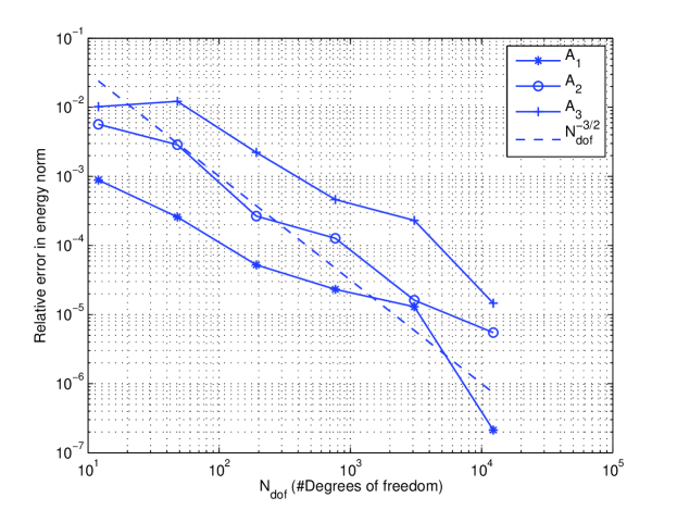
Refer to caption
Figure 5: Relative energy-norm error against Ndofsubscript𝑁dofN_{\text{dof}}, for C=2𝐶2C=2 in the localisation parameter L𝐿L for the the diffusion coefficients A1subscript𝐴1A_{1}, A2subscript𝐴2A_{2}, and A3subscript𝐴3A_{3}.

5.3 L2superscript𝐿2L^{2}-norm convergence

Again, set L=2log(H1)𝐿2superscript𝐻1L=\lceil 2\log(H^{-1})\rceil. Figure 6 and Figure 7, shows the relative L2superscript𝐿2L^{2}-norm error again the number of degrees of freedom between, uhsubscript𝑢u_{h} and uH,hLsuperscriptsubscript𝑢𝐻𝐿u_{H,h}^{L} and between uhsubscript𝑢u_{h} and ΠHuH,hLsubscriptΠ𝐻superscriptsubscript𝑢𝐻𝐿\Pi_{H}u_{H,h}^{L}, viz., uhΠHuHms,LL2(Ω)/uhL2(Ω)subscriptnormsubscript𝑢subscriptΠ𝐻superscriptsubscript𝑢𝐻𝑚𝑠𝐿superscript𝐿2Ωsubscriptnormsubscript𝑢superscript𝐿2Ω\|u_{h}-\Pi_{H}u_{H}^{ms,L}\|_{L^{2}(\Omega)}/\|u_{h}\|_{L^{2}(\Omega)}, respectively. In Figure 6 we see that the L2superscript𝐿2L^{2}-norm error between uhsubscript𝑢u_{h} and uHms,Lsuperscriptsubscript𝑢𝐻𝑚𝑠𝐿u_{H}^{ms,L} converges at a faster rate than in the energy norm (convergence rate 22-2 compared to 3/232-3/2, respectively,) as expected from (4.26). In Figure 7 only the coarse part of uHms,Lsuperscriptsubscript𝑢𝐻𝑚𝑠𝐿u_{H}^{ms,L} is used (i.e. ΠHuHms,LsubscriptΠ𝐻superscriptsubscript𝑢𝐻𝑚𝑠𝐿\Pi_{H}u_{H}^{ms,L}); nevertheless it appears to have a faster convergence rate than 1/212-1/2, except for the case of the permeability A3subscript𝐴3A_{3}.

Refer to caption
Figure 6: Relative L2superscript𝐿2L^{2}-norm error against Ndofsubscript𝑁dofN_{\text{dof}}, for C=2𝐶2C=2 in the localisation parameter L𝐿L for the the diffusion coefficients A1subscript𝐴1A_{1}, A2subscript𝐴2A_{2}, and A3subscript𝐴3A_{3}.
Refer to caption
Figure 7: Relative L2superscript𝐿2L^{2}-norm error against Ndofsubscript𝑁dofN_{\text{dof}}, for C=2𝐶2C=2 in the localisation parameter L𝐿L for the the diffusion coefficients A1subscript𝐴1A_{1}, A2subscript𝐴2A_{2}, and A3subscript𝐴3A_{3}.

References

  • [1] D. N. Arnold, An interior penalty finite element method with discontinuous elements, SIAM J. Numer. Anal. 19 (1982), no. 4, 742–760.
  • [2] I. Babuška, G. Caloz, and J. E. Osborn, Special finite element methods for a class of second order elliptic problems with rough coefficients, SIAM J. Numer. Anal. 31 (1994), no. 4, 945–981.
  • [3] I. Babuška and R. Lipton, The penetration function and its application to microscale problems, Multiscale Model. Simul. 9 (2011), no. 1, 373–406.
  • [4] I. Babuška and J. E. Osborn, Generalized finite element methods: their performance and their relation to mixed methods, SIAM J. Numer. Anal. 20 (1983), no. 3, 510–536.
  • [5] L. Berlyand and H. Owhadi, Flux norm approach to finite dimensional homogenization approximations with non-separated scales and high contrast, Arch. Ration. Mech. Anal. 198 (2010), no. 2, 677–721.
  • [6] F. Brezzi, L.P. Franca, T.J.R. Hughes, and A. Russo, b=g𝑏𝑔b=\int g, Comput. Methods Appl. Mech. Engrg. 145 (1997), 329–339.
  • [7] J. Douglas and T. Dupont, Interior penalty procedures for elliptic and parabolic Galerkin methods, Computing methods in applied sciences (Second Internat. Sympos., Versailles, 1975), Springer, Berlin, 1976, pp. 207–216. Lecture Notes in Phys., Vol. 58. MR 0440955 (55 #13823)
  • [8] D. Elfverson, E. Georgoulis, and A. Målqvist, An adaptive discontinuous galerkin multiscale method for elliptic problems, Submitted for publication (2012).
  • [9] T. Y. Hou and X.-H. Wu, A multiscale finite element method for elliptic problems in composite materials and porous media, J. Comput. Phys. 134 (1997), no. 1, 169–189.
  • [10] P. Houston, D. Schötzau, and T. P. Wihler, Energy norm a posteriori error estimation of hp𝑝hp-adaptive discontinuous Galerkin methods for elliptic problems, Math. Models Methods Appl. Sci. 17 (2007), no. 1, 33–62. MR 2290408 (2008a:65216)
  • [11] T. J. R. Hughes, G. R. Feijóo, L. Mazzei, and J.-B. Quincy, The variational multiscale method—a paradigm for computational mechanics, Comput. Methods Appl. Mech. Engrg. 166 (1998), no. 1-2, 3–24.
  • [12] O. Karakashian and F. Pascal, A posteriori error estimates for a discontinuous Galerkin approximation of second-order elliptic problems, SIAM J. Numer. Anal. 41 (2003), 2374–2399.
  • [13] M. G. Larson and A. Målqvist, Adaptive variational multiscale methods based on a posteriori error estimation: Energy norm estimates for elliptic problems, Computer Methods in Applied Mechanics and Engineering 196 (2007), no. 21-24, 2313–2324.
  • [14] A. Målqvist and D. Peterseim, Localization of elliptic multiscale problems, Submitted for publication in Math. Comp., in revision, available as preprint arXiv:1110.0692 (2011).
  • [15] A. Målqvist, Multiscale methods for elliptic problems, Multiscale Modeling & Simulation 9 (2011), no. 3, 1064–1086.
  • [16] H. Owhadi and L. Zhang, Localized bases for finite-dimensional homogenization approximations with nonseparated scales and high contrast, Multiscale Modeling & Simulation 9 (2011), no. 4, 1373–1398.

Appendix A Equalities for averages and jump operators

We derive equalities for averages and jump operators across interfaces where the functions v𝑣v and w𝑤w have discontinuities. Using [vw]={v}[w]+[v]{w}delimited-[]𝑣𝑤𝑣delimited-[]𝑤delimited-[]𝑣𝑤[vw]=\{v\}[w]+[v]\{w\} and {v}{w}={vw}1/4[v][w]𝑣𝑤𝑣𝑤14delimited-[]𝑣delimited-[]𝑤\{v\}\{w\}=\{vw\}-1/4[v][w], we have

{vw}[vu]=𝑣𝑤delimited-[]𝑣𝑢absent\displaystyle\{vw\}[vu]= {w}{v}[vu]+1/4[v][w][vu]𝑤𝑣delimited-[]𝑣𝑢14delimited-[]𝑣delimited-[]𝑤delimited-[]𝑣𝑢\displaystyle\{w\}\{v\}[vu]+1/4[v][w][vu] (A.1)
=\displaystyle= {w}[v2u]{w}[v]{vu}+1/4[v][w][vu]𝑤delimited-[]superscript𝑣2𝑢𝑤delimited-[]𝑣𝑣𝑢14delimited-[]𝑣delimited-[]𝑤delimited-[]𝑣𝑢\displaystyle\{w\}[v^{2}u]-\{w\}[v]\{vu\}+1/4[v][w][vu]
=\displaystyle= {w}[vu][v]{w}{v}{u}1/4[v]{w}[v][u]𝑤delimited-[]𝑣𝑢delimited-[]𝑣𝑤𝑣𝑢14delimited-[]𝑣𝑤delimited-[]𝑣delimited-[]𝑢\displaystyle\{w\}[vu]-[v]\{w\}\{v\}\{u\}-1/4[v]\{w\}[v][u]
+1/4[v]2[w]{u}+1/4[v]{v}[w][u]14superscriptdelimited-[]𝑣2delimited-[]𝑤𝑢14delimited-[]𝑣𝑣delimited-[]𝑤delimited-[]𝑢\displaystyle\quad+1/4[v]^{2}[w]\{u\}+1/4[v]\{v\}[w][u]

and

{vw}[vu]=𝑣𝑤delimited-[]𝑣𝑢absent\displaystyle\{vw\}[vu]= {v}{vw}[u]+{vw}[v]{u}𝑣𝑣𝑤delimited-[]𝑢𝑣𝑤delimited-[]𝑣𝑢\displaystyle\{v\}\{vw\}[u]+\{vw\}[v]\{u\} (A.2)
=\displaystyle= {v2w}[u]1/4[v][vw][u]+{vw}[v]{u}superscript𝑣2𝑤delimited-[]𝑢14delimited-[]𝑣delimited-[]𝑣𝑤delimited-[]𝑢𝑣𝑤delimited-[]𝑣𝑢\displaystyle\{v^{2}w\}[u]-1/4[v][vw][u]+\{vw\}[v]\{u\}
=\displaystyle= {v2w}[u]1/4[v]2{w}[u]1/4[v]{v}[w][u]superscript𝑣2𝑤delimited-[]𝑢14superscriptdelimited-[]𝑣2𝑤delimited-[]𝑢14delimited-[]𝑣𝑣delimited-[]𝑤delimited-[]𝑢\displaystyle\{v^{2}w\}[u]-1/4[v]^{2}\{w\}[u]-1/4[v]\{v\}[w][u]
+[v]{v}{w}{u}+1/4[v]2[w]{u}delimited-[]𝑣𝑣𝑤𝑢14superscriptdelimited-[]𝑣2delimited-[]𝑤𝑢\displaystyle\quad+[v]\{v\}\{w\}\{u\}+1/4[v]^{2}[w]\{u\}

Combining (A.1) and (A.2) we obtain

2{vw}[vu]={w}[v2u]+{v2w}[u]+1/2[v]2[w]{u}1/2[v]2{w}[u]2𝑣𝑤delimited-[]𝑣𝑢𝑤delimited-[]superscript𝑣2𝑢superscript𝑣2𝑤delimited-[]𝑢12superscriptdelimited-[]𝑣2delimited-[]𝑤𝑢12superscriptdelimited-[]𝑣2𝑤delimited-[]𝑢\displaystyle 2\{vw\}[vu]=\{w\}[v^{2}u]+\{v^{2}w\}[u]+1/2[v]^{2}[w]\{u\}-1/2[v]^{2}\{w\}[u] (A.3)

Also,

[vu][vu]=delimited-[]𝑣𝑢delimited-[]𝑣𝑢absent\displaystyle[vu][vu]= [u]{v}[vu]+[v]{u}[vu]delimited-[]𝑢𝑣delimited-[]𝑣𝑢delimited-[]𝑣𝑢delimited-[]𝑣𝑢\displaystyle[u]\{v\}[vu]+[v]\{u\}[vu] (A.4)
=\displaystyle= [u][v2u][v][u]{vu}+[v]{u}[vu]delimited-[]𝑢delimited-[]superscript𝑣2𝑢delimited-[]𝑣delimited-[]𝑢𝑣𝑢delimited-[]𝑣𝑢delimited-[]𝑣𝑢\displaystyle[u][v^{2}u]-[v][u]\{vu\}+[v]\{u\}[vu]
=\displaystyle= [u][v2u])[v][u]{v}{u}1/4[v][u][v][u]\displaystyle[u][v^{2}u])-[v][u]\{v\}\{u\}-1/4[v][u][v][u]
+[v]{u}[v]{u}+[v]{u}{v}[u]delimited-[]𝑣𝑢delimited-[]𝑣𝑢delimited-[]𝑣𝑢𝑣delimited-[]𝑢\displaystyle\quad+[v]\{u\}[v]\{u\}+[v]\{u\}\{v\}[u]
=\displaystyle= [u][v2u]1/4[v]2[u]2+[v]2{u}2delimited-[]𝑢delimited-[]superscript𝑣2𝑢14superscriptdelimited-[]𝑣2superscriptdelimited-[]𝑢2superscriptdelimited-[]𝑣2superscript𝑢2\displaystyle[u][v^{2}u]-1/4[v]^{2}[u]^{2}+[v]^{2}\{u\}^{2}