A study of non-keplerian velocities in observations of spectroscopic binary stars

Abstract

This paper presents an orbital analysis of six southern single-lined spectroscopic binary systems. The systems selected were shown to have circular or nearly circular orbits ($e<0.1$) from earlier published solutions of only moderate precision. The purpose was to obtain high precision orbital solutions in order to investigate the presence of small non-keplerian velocity effects in the data and hence the reality of the small eccentricities found for most of the stars.

The Hercules spectrograph and 1-m McLellan telescope at Mt John Observatory, New Zealand, were used to obtain over 450 CCD spectra between 2004 October and 2007 August. Radial velocities were obtained by cross correlation. These data were used to achieve high precision orbital solutions for all the systems studied, sometimes with solutions up to about 50 times more precise than those from the earlier literature. However, the precision of the solutions is limited in some cases by the rotational velocity or chromospheric activity of the stars.

The data for the six binaries analysed here are combined with those for six stars analysed earlier by Komonjinda et al. (2011). We have performed tests using the prescription of Lucy (2005) on all 12 binaries, and conclude that, with one exception, none of the small eccentricities found by fitting keplerian orbits to the radial-velocity data can be supported. Instead we conclude that small non-keplerian effects, which are clearly detectable for six of our stars, make impossible the precise determination of spectroscopic binary orbital eccentricities for many late-type stars to better than about 0.03 in eccentricity, unless the systematic perturbations are also carefully modelled. The magnitudes of the non-keplerian velocity variations are given quantitatively.

1 Introduction

This paper presents an analysis of six southern spectroscopic binary stars which have been analysed using high precision radial-velocity measurements derived from the cross-correlation of échelle spectra obtained with the Hercules fibre-fed vacuum spectrograph at Mt John Observatory.

The work continues the programme reported by Komonjinda et al. (2011) on single-lined spectroscopic binaries with circular or nearly circular orbits. The data are used to investigate the possibility that small non-keplerian velocities have produced a spurious eccentricity for a binary star with a circularized orbit, as claimed by Lucy (2005), even for apparent eccentricities as small as $e\sim 0.01$. The possible nature of non-keplerian perturbations is discussed in Section 6; in general they can arise whenever the flux-weighted mean radial velocity of the observed hemisphere of a star differs from the star’s centre-of-mass radial velocity.

Lucy (2005) has shown that such perturbations can in principle be detected by analysing the amplitude and phase of the third harmonic in an harmonic analysis of the velocity variations. In general non-keplerian perturbations, which may affect the second harmonic, cannot be distinguished from an eccentric keplerian orbit. However the amplitude and phase of the third harmonic must be consistent with the second harmonic if the variations are purely keplerian. Given that the keplerian third harmonic goes as $e^{2}$ ($e$ is the eccentricity) it follows that stars with circular or nearly circular orbits will have very small keplerian third harmonic terms, which makes it easier to detect a non-keplerian third harmonic. Our strategy is therefore to select bright southern late-type SB1 binaries from the literature known to have small eccentricities from earlier publications.

The idea of non-keplerian perturbations of spectroscopic binary velocities is far from new, and both Luyten (1936) and Sterne (1941a) considered the likely spurious eccentricities that would arise. In particular, Sterne (1941a) concluded that the tidal distortion of co-rotating stars could account for this effect, as it could lead to small line asymmetries and hence radial-velocity perturbations. Struve (1950) also suggested that spotted stars rotating synchronously with the orbital motion could result in a similar effect, without giving any quantitative analysis.

The work of Lucy & Sweeney (1971) devised a statistical test for the eccentricities of spectroscopic binaries, and concluded that over 100 of the binary orbits then in the literature with small non-zero eccentricities in reality failed the test, and their orbits were really circular. Following the work of Lucy & Sweeney (1971), Monet (1979) emphasized the benefit of harmonic analysis by determining the second and higher harmonics in radial velocity curves. He concluded that at least four of the nine early-type binaries that he analysed have circular orbits, in spite of a published eccentricity in one case as high as $e=0.09$.

The issue of small eccentricities is re-tackled here, because the collection of much higher precision data is now possible using stable spectrographs and CCD detectors, thus making the detection of apparently significant eccentricities with $e<0.01$. By carefully selecting stars known to have nearly circular or circular orbits, we have been able to show that very small non-keplerian effects can indeed be detected at the level of $<10$ m s^-1 in the third harmonic.

The present programme selected six spectroscopic binaries from the Ninth catalogue of spectroscopic binary orbits, $S_{B^{9}}$ (Pourbaix et al., 2004), which contains over 3300 orbital solutions for 2770 binaries. The selection criteria were that the earlier analysis reported an eccentricity $e<0.1$, with F, G or K spectral type for the primary star, with a southern declination ($\delta<0^{\circ}$) and brighter than $m_{V}=8.0$. In addition systems with rather long periods ($P>850$ d) or very short periods ($P<2.2$ d) were also excluded, and three stars with high levels of chromospheric activity and large $v\sin i$ were also not included. Only 11 binary systems satisfied all these selection criteria. One additional system, HD 101379 (GT Muscae), which was strangely not listed in $S_{B^{9}}$, but which otherwise satisfies the criteria, was also included in this programme. Its orbit was analysed earlier by Murdoch et al. (1995). This paper reports the results for six systems (including GT Muscae). Together with those analysed by Komonjinda et al. (2011) this brings the total to 12 systems selected, being all those satisfying the criteria. All are late-type evolved stars.

Table 1 lists the six objects selected for observation and analysis in this paper.

Table 1: The six selected spectroscopic binaries studied in this paper. All the stars are listed in $S_{B^{9}}$ except for HD 101379.

HD	RA(2000.0)	Dec(2000.0)	$m_{V}$	Spectral type	$P$ (days)
77258	09 00 05.44	–41 15 13.5	4.45	G8-K1III	74.1469
85622	09 51 40.69	–46 32 51.5	4.57	G5Ib	329.3
101379	11 39 29.59	–65 23 51.9	5.17	G2III	61.448
124425	14 13 40.67	–00 50 42.4	5.93	F6IV	2.696
136905	15 23 26.06	–06 36 36.7	7.31	K1III	11.1345
194215	20 25 26.82	–28 39 47.8	5.84	G8II/III	377.6

2 Observations and statistics

The observational part of this research was carried out at Mt John University Observatory (New Zealand) from 2004 October to 2007 August. All observations were carried out on the 1-m McLellan telescope, using the Hercules fibre-fed vacuum échelle spectrograph (Hearnshaw et al., 2002). Relevant details of the observing procedure are given by Komonjinda et al. (2011). For all stars a resolving power of 70 000 was used, except for HD 136905, where $R=41\,000$ was adopted, as this star is somewhat fainter than the others. A typical signal-to-noise ratio of $\sim 100:1$ was obtained for our spectra in a pixel-column.

The Hercules detector mainly used was a SITe SI 003 1024$\times$1024 thinned CCD chip with 24-micron square pixels. (In Komonjinda et al. (2011) this was incorrectly given as 23-micron pixels.) This chip cannot cover all the focal plane area of the dispersed spectrum, but was positioned so as to cover 46 orders from 457 to 722 nm (orders 79 to 124). Later in 2006, the detector for Hercules was changed to a Spectral Instruments camera with a Fairchild 486 CCD which has 4096$\times$4096 15-micron square pixels. This was only used for two runs in 2007 August.

3 Data reduction and radial-velocity determination

All the spectra obtained were reduced using the Hercules Reduction Software Package, HRSP version 2.3 (Skuljan, 2003). This software is a C program running under Linux. The dispersion solution was obtained from two thorium-argon lamp spectra, recorded immediately before and after each stellar spectrum. About 400 Th or Ar lines were used. Further details are given by Komonjinda et al. (2011).

All radial velocities were determined by cross correlation for the 30 échelle orders used, using one chosen spectrum of the same star as a template relative to which all other spectra of that star were measured, and following the Fourier cross-correlation techniques pioneered by Simkin (1974) for digital spectra. In particular, the cross-correlation was performed in $\ln\lambda$ space after subtracting the mean flux from each spectrum and applying a cosine bell to the ends of the data window. The position of the cross-correlation function (CCF) peak was determined by means of a gaussian least squares fit, typically using eight consecutive data points spanning the peak.

4 Orbit analysis from radial velocities

The six orbital elements of a particular binary system, $K$ (radial-velocity semi-amplitude), $e$ (orbital eccentricity), $\omega$ (longitude of periastron), $T_{0}$ (time of zero mean longitude), $P$ (period) and $\gamma$ (the centre-of-mass radial velocity), can be determined from a set of $n$ observations of radial velocity $V_{\mathrm{rad}}(t)$. The best values of these elements can be found following an iterative least-squares analysis involving differential corrections, based on the method of Lehmann-Filhés (1894). Data points lying more than $3\sigma$ from the fitted solution have been rejected and the remaining points then used for a second solution; rejected points are still plotted in the figures and they appear in the tables of measured radial velocities.

Here we use a software package SpecBin written by J. Skuljan (Skuljan et al., 2004). Since the orbits here are close to being circular, the variation of the Lehmann-Filhés procedure described by Sterne (1941b) was adopted, unless otherwise stated. This makes use of the time of zero mean longitude ($T_{0}$) instead of the poorly determined time of periastron passage ($T$). The mean longitude is given by $L=2\pi(t-T)/P+\omega$ and hence the time when $L$ is zero is $T_{0}=T-\omega P/2\pi$. In fact, for one star there is a well-determined non-zero eccentricity (HD 194215), so for this star we were able reliably to determine the time of periastron passage, and hence we used that time for the phase zero-point.

Since our radial velocities are relative to a template observation of the same star, our orbital solutions quote $\gamma_{\rm rel}$. In addition our solutions from Hercules data give an absolute centre-of-mass velocity, $\gamma$, of lower accuracy, based on cross-correlating the template with a standard star. Further details of SpecBin and the process of estimating the error bars in the orbital elements are discussed by Skuljan et al. (2004).

We have also used SpecBin to reanalyse the historical data for the stars in the literature. This has allowed us to compare $T_{0}$ values from the historical data with those from our data, and hence to derive better periods (for four of the stars) than from either data set alone, using the long time base line.

5 Results of the analysis for individual stars

In this section the results of the orbital analysis of each of the binary systems are presented.

5.1 HD 77258

The bright star HD 77258 (w Velorum, HR 3591) was first observed to have a variation in radial velocity by H.K. Palmer, as reported in the Lick Observatory Bulletin in 1904 (Wright, 1904).

The spectral type was classified as F8IV by de Vaucouleurs (1957), but it is given as G8-K1III+A in the Michigan Spectral Catalogue (Houk, 1982). The Hipparcos photometry of HD 77258 shows that no detectable light variation was present. The parallax of this system in the Hipparcos main catalogue is $16.19\pm 0.53$ mas, which implies a distance of $61.8\pm 2.0$ pc. The absolute magnitude is $M_{V}=+0.50$, supporting the giant luminosity class.

Lunt (1919) observed five spectra of HD 77258 at the Cape during 1914–1916. He showed that the star has a range in radial velocity of 34.2 km s^-1. During February and May 1921, 38 further spectra were observed and the radial velocities were used for an orbital solution of low precision (root mean square residual of 1.23 km s^-1), as reported by Lunt (1924).

The Hercules radial velocities for HD 77258 were measured from 101 spectra and are given in Table 11. The orbital solution found has an rms scatter of 19 m s^-1, which is comparable with the lowest scatter in radial velocities for sharp-lined stars observed with Hercules.

The orbital parameters are presented in Table 2. Figure 1 is a plot of these radial velocities as a function of (a) orbital phase and (b) Julian Date. The orbital phase is calculated from the period of 74.13715 days and the zero phase is defined by $T_{0}=\mathrm{JD}\,245\,3625.5112\pm 0.0017$, the time of zero mean longitude.

Table 2: The orbital parameters of SB1 HD 77258 (F8IV) as obtained from Hercules data.

Parameter	Hercules solutions
	no fixed parameter	when $P$ = $\bar{P}$
K (km s-1)	19.6744 $\pm$ 0.0041	19.6747 $\pm$ 0.0039
e	0.000 85 $\pm$ 0.000 19	0.000 87 $\pm$ 0.000 19
$\omega$ (∘)	106 $\pm$ 13	106 $\pm$ 12
$T_{0}$ (HJD)	245 3625.5112$\pm$ 0.0017	245 3625.5113 $\pm$ 0.0017
P (days)	74.137 15 $\pm$ 0.000 73	74.1368 (fixed)
$\gamma_{\mathrm{rel}}$ (km s-1)	18.2758 $\pm$ 0.0027	18.2757 $\pm$ 0.0027
$\gamma$ (km s-1)	$-$5.0133 $\pm$ 0.042	$-$5.0134 $\pm$ 0.042
$\#_{obs}$	101	101
$\#_{rej}$	10	10
$\sigma$ (km s-1)	0.019	0.019
$a_{1}\sin i$ ($\times 10^{7}$ km)	$2.0057\pm 0.0004$	$2.0057\pm 0.0005$
$f(M)$ ($M_{\odot}$)	$0.058498\pm 0.000037$	$0.058500\pm 0.000037$

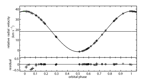
(a) Phase plot of HD 77258 radial velocities.

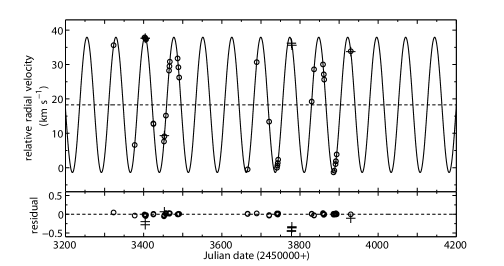
(b) Measured radial velocities of HD 77258 versus Julian date.

Figure 1: Radial velocities of HD 77258 measured from the Hercules spectra. The plotted curves are calculated from the orbital solution calculated from these radial velocities with all free parameters. The second panel of each figure shows the residuals from the fit. Open circles are points used in the orbital solution, and the crosses (+) are rejected points with residuals of at least $3\sigma$.

The period calculated from $T_{0}$ from the combined data of Lunt (1924) and from the Hercules data is $\bar{P}=74.1368\pm 0.0023$ days. This period has a lower precision than the period that was calculated from the Hercules data alone (in spite of about eight decades of baseline between the two times of data collection). Table 2 also shows the solution with the period fixed using the combined data set; it differs negligibly from the solution from Hercules data alone.

5.2 HD 85622

HD 85622 (m Velorum, HR 3912) is a system with a supergiant primary star. It was first found to have variable radial velocity in 1905 during the D.O. Mills Expedition (Wright, 1907). It was classified as a supergiant star of spectral type G5Ib by MacConnell & Bidelman (1976). The rotational velocity, $v\sin i$, of the supergiant component was measured by de Medeiros et al. (2002) as $19.3\pm 1.0$ km s^-1.

The Hipparcos and Tycho photometry indicated that this system has a micro-variability in its brightness with 0$\stackrel{{\scriptstyle\raise 0.90417pt\hbox{\scriptsize m}}}{{\lower 0.21529pt\hbox{.}}}$007 scatter in $H_{p}=4\hbox{$\stackrel{{\scriptstyle\raise 0.90417pt\hbox{\scriptsize m}}}{{\lower 0.21529pt\hbox{.}}}$}749\pm 0\hbox{$\stackrel{{\scriptstyle\raise 0.90417pt\hbox{\scriptsize m}}}{{\lower 0.21529pt\hbox{.}}}$}0007$ and 0$\stackrel{{\scriptstyle\raise 0.90417pt\hbox{\scriptsize m}}}{{\lower 0.21529pt\hbox{.}}}$023 scatter in $V_{T}=4\hbox{$\stackrel{{\scriptstyle\raise 0.90417pt\hbox{\scriptsize m}}}{{\lower 0.21529pt\hbox{.}}}$}713\pm 0\hbox{$\stackrel{{\scriptstyle\raise 0.90417pt\hbox{\scriptsize m}}}{{\lower 0.21529pt\hbox{.}}}$}002$. In other words the intrinsic variability is about ten times larger than the standard error of photometric measurement.

Luyten (1936) collected 56 radial-velocity observations of HD 85622 from the papers by Lunt (1919) and Jones (1928). He adopted a circular orbit for this system with an rms residual of 1.4 km s^-1.

Eighty-six radial velocities were measured from the Hercules spectra obtained. It was found that the calculated eccentricity has a large error bar, $e=0.0026\pm 0.0016$. A circular orbit should therefore be adopted from these data with a precision of 61 m s^-1. These two solutions, with the eccentricity floating or fixed to zero, can be compared in Table 3.

The radial velocities of this system and the residuals for the circular orbital solution are plotted versus orbital phase in Fig. 2 (a) and versus Julian date in Fig. 2(b). The zero phase is at the time $T_{0}=\mathrm{JD}\,245\,3860.281\pm 0.074$.

Table 3: The orbital parameters of SB1 HD 85622 analysed from Hercules data.

Parameter	Hercules solutions
	eccentric orbit	circular orbit
K (km s-1)	13.028 $\pm$ 0.013	13.021 $\pm$ 0.012
e	0.0026 $\pm$ 0.0016	0 (adopted)
$\omega$ (∘)	188 $\pm$ 46	–
$T_{0}$ (HJD)	245 3860.261 $\pm$ 0.078	245 3860.281 $\pm$ 0.074
P (days)	329.126 $\pm$ 0.093	329.266 $\pm$ 0.085
$\gamma_{\mathrm{rel}}$ (km s-1)	$-$11.516 $\pm$ 0.013	$-$11.531 $\pm$ 0.010
$\gamma$ (km s-1)	11.510 $\pm$ 0.037	11.495 $\pm$ 0.034
$\#_{obs}$	86	86
$\#_{rej}$	6	6
$\sigma$ (km s-1)	0.060	0.061
$a_{1}\sin i$ ($\times 10^{7}$ km)	$5.8962\pm 0.0076$	$5.8956\pm 0.0076$
$f(M)$ ($M_{\odot}$)	$0.07540\pm 0.00025$	$0.07532\pm 0.00023$

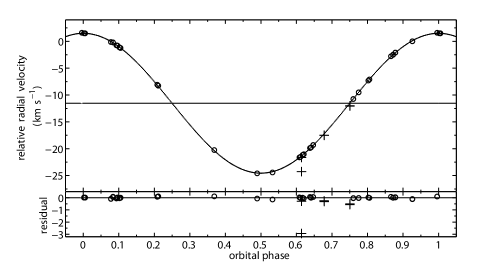
(a) Phase plot of HD 85622 radial velocities.

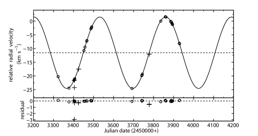
(b) Measured radial velocities of HD 85622 versus Julian date.

Figure 2: Radial velocities of HD 85622 measured from the Hercules spectra. The plotted curves are calculated from the circular orbital solution. The second panel shown the residuals from this fit.

5.3 HD 101379

HD 101379 or GT Muscae is a member of a quadruple system. The brightness is variable, because the system comprises an RS CVn-type single-lined spectroscopic binary, HD 101379 (orbital period $\sim 61.4$ d) and the eclipsing binary, HD 101380 (eclipsing period $\sim 2.75459$ d). McAlister et al. (1990) reported the separation between the two components as 0.23 arcsec from speckle interferometry.

The spectral types of the stars in this system have been classified by many authors. Houk & Cowley (1975) have classified HD 101379 as G5/G8III and HD 101380 as A0/1V. Collier (1982) determined the spectral types of HD 101379 as K4III and of the components of the eclipsing system as A0V and A2V from his photometric analysis.

The RS CVn-type system HD 101379 shows a strong CaII H and K emission and a variable H$\alpha$ line (Collier et al., 1982).

An analysis of GT Mus spectra was done by Murdoch et al. (1995). In that paper, the orbital solution of the system HD 101379 was analysed from the 17 spectra that were obtained from the MJUO’s Cassegrain échelle spectrograph linked with the McLellan 1-m telescope, which were combined with other radial velocities reported by Balona (1987), Collier Cameron (1987) and MacQueen (1986).

In this study, 76 high resolution spectra of GT Mus at a wavelength 450–720 nm were obtained from the Hercules spectrograph. These spectra, which are dominated by HD 101379, were obtained over a period of two years (2004 October – 2006 June) with a signal-to-noise ratio of typically 70. Relative radial velocities of these spectra were calculated using the cross-correlation technique with a template spectrum. These relative radial velocities of HD 101379 can be converted into absolute radial velocities using the relative radial velocity of the template spectrum with respect to a standard star spectrum. The spectrum of the standard star HD 109379 (G5II) was used for this purpose. The relative radial velocity of the template with respect to this standard star is $21.110\pm 0.024$ km s^-1. The standard star absolute velocity is $-7.246\pm 0.024$ km s^-1, as obtained by Ramm (2004).

The orbital solution was calculated using the above radial velocities. The solution, as in Table 4, has an rms of 518 m s^-1. This is three times larger than the precision of the Murdoch et al. (1995) radial velocities, for the reasons discussed below.

Table 4: The orbital parameters of SB1 HD 101379 (G5/8III) derived from Hercules radial velocities, and from Hercules data combined with previously published radial velocities.

Parameter	New analysed values	Combined data
	Hercules data only
K (km s-1)	12.911 $\pm$ 0.078	$12.823\pm 0.049$
e	0.012 $\pm$ 0.010	$0.0053\pm 0.0034$
$\omega$ (∘)	$237\pm 51$	$73\pm 51$
$T_{0}$ (HJD)	245 3736.00 $\pm$ 0.10	$244\,4951.03\pm 0.13$
P (days)	61.408 $\pm$ 0.027	$61.4370\pm 0.0012$
$\gamma$ (km s-1)	1.02 $\pm$ 0.11
$\#_{obs}$	76	183
$\#_{rej}$	0	1
$\sigma$ (km s-1)	0.518	0.380
$a_{1}\sin i$ ($\times 10^{7}$ km)	$1.0902\pm 0.0071$	$1.0833\pm 0.0042$
$f(M)$ ($M_{\odot}$)	$0.01369\pm 0.00025$	$0.01342\pm 0.00015$

Fig. 3a and b show the relative radial velocities measured from the Hercules spectra with their residuals in the second panel. It is clearly seen that the residuals from this fit have a positive value during the first observation period and have a negative value during the second period. This should be due to the fact that the system GT Mus is a quadruple system, with HD 101379 showing long-period orbital motion with its companion, HD 101380. This long scale variation was not shown in the radial velocities of Murdoch et al. (1995) because of their shorter observation window (JD 244 8260 – 244 8479).

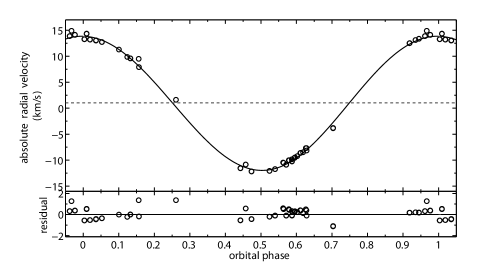
(a) Phase plot of HD 101379 radial velocities.

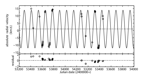
(b) Measured radial velocities of HD 101379 versus Julian date.

Figure 3: Radial-velocity observations of GT Mus measured from Hercules spectra. The plotted curves are calculated from the orbital solution calculated from these radial velocities. The second panels show the residuals from the fits.

When these data are separated into two groups by the observation time (2004 October – 2005 May and 2005 November – 2006 June), each data set gave a better solution, with rms residuals of 79 m s^-1 and 54 m s^-1 respectively, as shown in Table 5.

Table 5: The orbital parameters of HD 101379 derived from two data sets of Hercules radial velocities, 2004 October – 2005 May and 2005 November – 2006 June.

Parameter	Hercules solutions
	2004 October – 2005 May	2005 November – 2006 June
K (km s-1)	12.948 $\pm$ 0.027	12.715 $\pm$ 0.011
e	0.0225 $\pm$ 0.0038	0.0331 $\pm$ 0.0027
$\omega$ (∘)	175.3 $\pm$ 6.9	61.8 $\pm$ 2.1
$T_{0}$ (HJD)	245 3429.478 $\pm$ 0.036	245 3797.763 $\pm$ 0.018
P (days)	61.516 $\pm$ 0.045	61.331 $\pm$ 0.017
$\gamma$ (km s-1)	1.723 $\pm$ 0.035	0.287 $\pm$ 0.026
$\#_{obs}$	34	42
$\#_{rej}$	1	1
$\sigma$ (km s-1)	0.079	0.054
$a_{1}\sin i$ ($\times 10^{7}$ km)	$1.0950\pm 0.0031$	$1.0717\pm 0.0017$
$f(M)$ ($M_{\odot}$)	$0.01383\pm 0.00010$	$0.01304\pm 0.00006$

The orbital solutions from both data sets do not change dramatically, except the longitude of periastron $\omega$ and the systemic radial velocity $\gamma$. The value of $\omega$ changed from $175\hbox{$\stackrel{{\scriptstyle\raise 0.90417pt\hbox{\scriptsize$\circ$}}}{{\lower 0.21529pt\hbox{.}}}$}3\pm 6\hbox{$\stackrel{{\scriptstyle\raise 0.90417pt\hbox{\scriptsize$\circ$}}}{{\lower 0.21529pt\hbox{.}}}$}9$ to $61\hbox{$\stackrel{{\scriptstyle\raise 0.90417pt\hbox{\scriptsize$\circ$}}}{{\lower 0.21529pt\hbox{.}}}$}8\pm 2\hbox{$\stackrel{{\scriptstyle\raise 0.90417pt\hbox{\scriptsize$\circ$}}}{{\lower 0.21529pt\hbox{.}}}$}1$ and the value of $\gamma$ changed from $1.723\pm 0.035$ to $0.287\pm 0.26$ km s^-1. These changes result respectively from the apsidal motion of HD 101379 caused by its companion system, HD 101380, and by the orbital motion of the visual pair around the centre of mass of the GT Mus quadruple system.

To improve the solution, the historical radial velocities were analysed together with Hercules radial velocities. The radial velocities of HD 101379 were observed and reported by several observers using different instruments. These include MacQueen (1986), Collier Cameron (1987) and Murdoch et al. (1995). The other observations of HD 101379 that are included in this analysis are from Balona (1987). The data from MacQueen (1986) could not be combined into this analysis, as his radial velocities showed an orbital period of around 54 days. The orbital solutions were calculated from all the other data sets.

Table 6: The systemic radial velocity $\gamma$ of HD 101379 calculated from historical radial velocities and Hercules radial velocities.

Radial velocity data	$T_{0}$	$\gamma$
	(HJD 2400000+)	(km s-1)
Balona (1987)	44 397.25 $\pm$ 0.63	9.12 $\pm$ 0.50
Collier Cameron (1987)	44 458.71 $\pm$ 0.59	8.13 $\pm$ 0.38
Murdoch et al. (1995)	48 391.76 $\pm$ 0.42	0.53 $\pm$ 0.47
Hercules data set 1	53 429.478 $\pm$ 0.036	1.723 $\pm$ 0.035
Hercules data set 2	53 797.763 $\pm$ 0.018	0.287 $\pm$ 0.026

The systemic radial velocities, $\gamma$, and times of zero mean longitude, $T_{0}$, of each data set are shown here in Table 6. These $\gamma$ values decrease during 30 years of observation. The orbital period of HD 101379 around the centre-of-mass of GT Mus cannot be calculated from these few data points. From the Hipparcos catalogue, the parallax is $5.81\pm 0.64$ mas and the separation between the two stars is $0.217\pm 0.004$ arcsec. The latter value is consistent with the interferometric measurement of McAlister et al. (1990). The HIP astrometry also measured the changing rate of the position angle between the two systems as $d\theta/dt=3\hbox{$\stackrel{{\scriptstyle\raise 0.90417pt\hbox{\scriptsize$\circ$}}}{{\lower 0.21529pt\hbox{.}}}$}0$ per year. This information gave a lower limit of the total system mass as $3.6M_{{}_{\odot}}$. This value is about a half of the total mass calculated from the components’ spectral types of G5III, M dwarf, A0V and A2V stars, of $7.4M_{{}_{\odot}}$.

The radial velocities from each data set were shifted to the zero point of $\gamma$. The final orbital solution was calculated from a data set containing all relative velocities with the data weighted in the ratio Balona:Collier Cameron:Murdoch:this work 0.02:0.08:0.7:1.0 in accordance with the calculated rms scatter of each data set solution. The period of a solution from these combined data was $61.4370\pm 0.0012$ days with an rms residual of 380 m s^-1. This orbital solution is shown in Table 4. Thus this orbital solution gives a higher precision for the period.

5.4 HD 124425

The solar neighbourhood star HD 124425 (HR 5317) is a short period spectroscopic binary ($P\approx 2.69$ days). It was found to have a variation in its radial velocity by A.M. Brayton in early 1920 using Mt Wilson 60-inch telescope spectra (Duncan, 1921).

The Hipparcos satellite photometry measured a magnitude of $H_{\rm p}=5\hbox{$\stackrel{{\scriptstyle\raise 0.90417pt\hbox{\scriptsize m}}}{{\lower 0.21529pt\hbox{.}}}$}9996\pm 0\hbox{$\stackrel{{\scriptstyle\raise 0.90417pt\hbox{\scriptsize m}}}{{\lower 0.21529pt\hbox{.}}}$}0006$ for this system and indicated that no variability was detected. The $V$ magnitude from the TYCHO photometry is $5\hbox{$\stackrel{{\scriptstyle\raise 0.90417pt\hbox{\scriptsize m}}}{{\lower 0.21529pt\hbox{.}}}$}948\pm 0\hbox{$\stackrel{{\scriptstyle\raise 0.90417pt\hbox{\scriptsize m}}}{{\lower 0.21529pt\hbox{.}}}$}004$.

HD 124425 was later observed by Mayor & Mazeh (1987) with the CORAVEL radial-velocity scanner at Haute-Provence Observatory between 1980 and 1982. They analysed 16 radial velocities with an assumed circular orbit and a fixed orbital period.

In this research, 64 Hercules spectra of HD 124425 were obtained. Table 7 is the orbital solution from these velocities, analysed using SpecBin. A very small and marginally significant eccentricity was obtained ($e=0.00260\pm 0.00099$). These radial velocities are plotted versus orbital phase in Fig. 4(a) and versus Julian Date in Fig. 4(b). The time of zero mean longitude in Table 7 ($T_{0}=245\,3800.308\,08$) was used for the zero point of phase. The lower panels of these figures show the residuals from the fitted solution. The rms residual velocity is 121 m s^-1.

Table 7: The new orbital parameters of SB1 HD 124425 (F6IV) analysed from Hercules spectra.

Parameter	Hercules solutions
	with all free parameters	with fixed $P$
K (km s-1)	26.094 $\pm$ 0.023	26.107 $\pm$ 0.023
e	0.002 60 $\pm$ 0.000 99	$0.002\,70\pm 0.000\,94$
$\omega$ (∘)	294 $\pm$ 26	306 $\pm$ 21
$T_{0}$ (HJD)	245 3800.308 08	245 3800.307 52
	$\pm$ 0.000 47	$\pm$ 0.000 40
P (days)	2.697 0329	2.697 0220 (fixed)
	$\pm$ 0.000 0050	–
$\gamma_{\mathrm{rel}}$ (km s-1)	$26.040\pm 0.015$	26.035 $\pm$ 0.016
$\gamma$ (km s-1)	18.684 $\pm$ 0.054	18.679 $\pm$ 0.055
$\#_{obs}$	64	64
$\#_{rej}$	1	1
$\sigma$ (km s-1)	0.121	0.126
$a_{1}\sin i$ ($\times 10^{7}$ km)	$0.096774\pm 0.000086$	$0.096822\pm 0.000085$
$f(M)$ ($M_{\odot}$)	$0.004965\pm 0.000013$	$0.004972\pm 0.000013$

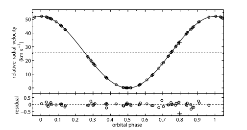
(a) Phase plot of HD 124425 radial velocities.

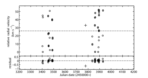
(b) Measured radial velocities of HD 124425 versus Julian date.

Figure 4: Radial velocities of HD 124425 measured from Hercules spectra. The second panels show the residuals from the fit with all free parameters as in table 7.

In order to get a higher precision for the orbital period, the number of orbital cycles was calculated to be $N_{c}=11\,515$ from the difference in $T_{0}$ of the recalculated solution of Duncan (1921) and the above Hercules solution. This gave $\bar{P}$ = 2.697 0220 $\pm$ 0.000 0024 or a precision of 0.2 second. This is half of the error in the orbital period of Mayor & Mazeh (1987), which they calculated in the same way. The orbital solution was recalculated with this fixed $\bar{P}$ and is also shown in Table 7.

5.5 HD 136905

The binary star HD 136905 (GX Librae) is an ellipsoidal variable with an active K giant. The star was first reported to have H and K emission by Bidelman & MacConnell (1973). They classified the star as a K1III+F system with the remark that the emission was uncertain. Burke et al. (1982) concluded from their spectroscopic and $UBV$ photometric observations that this system is an RS CVn-type binary of spectral type K0III-IV and with a moderate emission at H and K.

Fekel et al. (1985) reported moderate strength Ca II H and K and ultraviolet emission features and a strong H$\alpha$ absorption. They suggested that HD 136905 is an ellipsoidal variable, as their light curve showed a frequency of twice the orbital frequency. They also found that the light curve has a variable amplitude and suggested that this could be the result of spot activity.

The Hipparcos photometry indicated that HD 136905 has an 11.12-day periodic variability of semi-amplitude about 0$\stackrel{{\scriptstyle\raise 0.90417pt\hbox{\scriptsize m}}}{{\lower 0.21529pt\hbox{.}}}$1. These variations are synchronous with the orbital period and therefore suggest the spot wave of a tidally locked co-rotating active chromosphere star. The $H_{p}$ magnitude (observed 1989–93) as well as the $V$ magnitude observed from Mt John photoelectric photometry (observed 2004–07) are plotted in Fig. 5. The shapes of the curves differ somewhat, and the semi-amplitude of the Mt John data is about 0$\stackrel{{\scriptstyle\raise 0.90417pt\hbox{\scriptsize m}}}{{\lower 0.21529pt\hbox{.}}}$05, which is comparable with the result of Kaye et al. (1995).

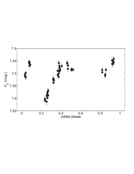
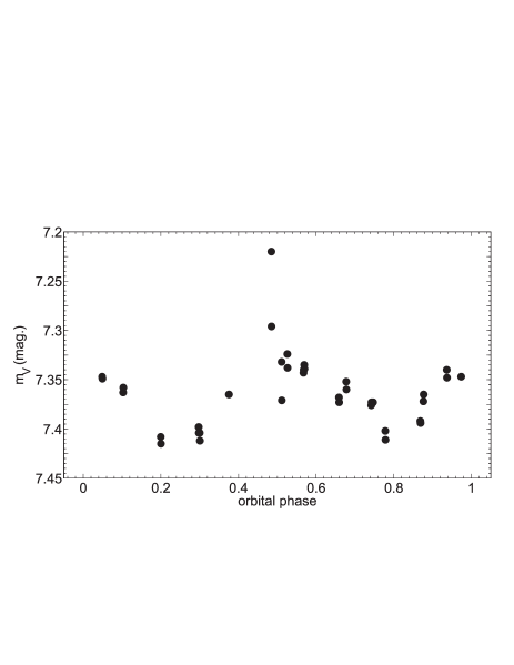
Figure 5: The light curves of the active chromosphere variable HD 136905 (a) from the Hipparcos satellite and (b) from Mt John Observatory. The orbital phase was calculated from the Hercules eccentric solution (Table 8).

Previous studies of the orbit of this system were by Fekel et al. (1985), by Balona (1987) and by Kaye et al. (1995). All these authors obtained circular orbits from data of only moderate precision.

Our observations with Hercules resulted in 42 spectra of HD 136905 with a resolving power of 41 000. The orbital solution is shown in Table 8. The plot of the radial-velocity curve from this solution is shown in Fig. 6 versus (a) orbital phase and (b) Julian date. The orbital phase is calculated from the period of an eccentric solution and we define the time of zero phase as $T_{0}=\mathrm{JD}\,245\,3599.1743\pm 0.0055$. The rms scatter is 326 m s^-1, which is high, as can be expected for an ellipsoidal RS CVn-type binary system.

Table 8: The orbital parameters of SB1 HD 136905 (K1III) analysed from Hercules radial velocities.

Parameter	Hercules solutions
	eccentric orbit	with $e=0$	with $P=\bar{P}$
K (km s-1)	39.029 $\pm$ 0.078	38.989 $\pm$ 0.082	39.040 $\pm$ 0.077
e	0.0079 $\pm$ 0.0026	0 (fixed)	0.0081 $\pm$ 0.0019
$\omega$ (∘)	23 $\pm$ 24	-	33 $\pm$ 17
$T_{0}$ (HJD)	245 3599.1743	245 3599.1715	245 3599.1717
	$\pm$ 0.0055	$\pm$ 0.0067	$\pm$ 0.0049
P (days)	11.134 14	11.134 13	11.134396 (fixed)
	$\pm$ 0.000 30	$\pm$ 0.00029
$\gamma_{\mathrm{rel}}$ (km s-1)	$-$10.116 $\pm$ 0.065	$-$10.055 $\pm$ 0.062	$-$10.095 $\pm$ 0.060
$\gamma$ (km s-1)	61.78 $\pm$ 0.14	61.72 $\pm$ 0.13	61.76 $\pm$ 0.13
$\#_{obs}$	42	42	42
$\#_{rej}$	0	0	0
$\sigma$ (km s-1)	0.326	0.385	0.325
$a_{1}\sin i$ ($\times 10^{7}$ km)	$0.5975\pm 0.0012$	$0.5969\pm 0.0012$	$0.5977\pm 0.0012$
$f(M)$ ($M_{\odot}$)	$0.06858\pm 0.00041$	$0.06837\pm 0.00043$	$0.06864\pm 0.00041$

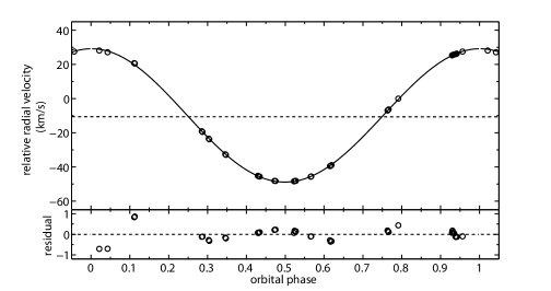
(a) Phase plot of HD 136905 radial velocities.

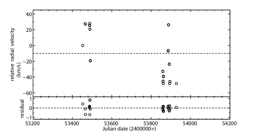
(b) Measured radial velocities of HD 136905 versus Julian date.

Figure 6: Radial velocities of HD 136905 measured from the Hercules spectra. The second panels show the residuals from that fit.

The long time span between the historical data-set and the recent Hercules spectra allows us to determine the orbital period of this system with a higher precision. The orbital period calculated from the $T_{0}$ values of the eccentric solutions of Kaye et al. (1995) and from Hercules data is $\bar{P}=11.134\,396\pm 0.000\,031$ days (an uncertainty of $\pm 2.7$ s). However the orbital solution using this more precise period differs negligibly from that derived from Hercules data alone, as seen from Table 8.

5.6 HD 194215

HD 194215 (HR 7801) is a single-lined spectroscopic binary system for which the primary has been variously classified as K0 (in the HD Catalogue), K3V (Buscombe, 1962) and G8II/III (Houk, 1982). The Hipparcos parallax of $6.50\pm 0.78$ mas gives $M_{V}=-0.10\pm 0.26$, so the primary star is clearly a giant. Buscombe & Morris (1958) noted that the radial velocity was variable. However, there is no evidence of a photometric variation from the Hipparcos photometry, the Hipparcos magnitude being $H_{\rm p}=6.0227\pm 0.0006$.

Bopp et al. (1970) measured 28 radial velocities of this system and analysed its orbit. The solution found is an eccentric orbit with $e=0.0687\pm 0.0138$ and $P=377.60\pm 0.25$ days. The rms scatter of their measurement is given as 2.2594 km s^-1(so many digits seem unnecessary!). Their data were reanalysed using SpecBin and it was found that the orbital solution was significantly different from the published solution, especially for the orbital period. It is possible that the solution or data reported by Bopp et al. (1970) contains a typographical or computational error, especially as their quoted value of $T$ lies far outside the time range of the observations.

In total, we have obtained 97 Hercules spectra of HD 194215. An eccentric orbital solution was calculated from the radial velocities measured from these spectra. This solution is shown in Table 9. The radial velocities are shown in Fig. 7 plotted versus (a) orbital phase and (b) Julian date. This eccentric solution has an rms scatter of the fit of 47 m s^-1. The time of periastron passage is $T=\mathrm{JD}\,245\,3918.52\pm 0.65$. For this star, we have chosen the zero point for phase to be the time of periastron.

Table 9: The orbital parameters of SB1 HD 194215 (G8II/III) analysed from Hercules radial velocities.

Parameter	Hercules solutions
	all free parameters
K (km s-1)	14.1155 $\pm$ 0.0056
e	0.123 29 $\pm$ 0.000 78
$\omega$ (∘)	258.14 $\pm$ 0.77
$T_{0}$ (HJD)	245 3649.711 $\pm$ 0.074
P (days)	374.88 $\pm$ 0.18
$\gamma_{\mathrm{rel}}$ (km s-1)	$-12.086\pm 0.022$
$\gamma$ (km s-1)	$-$8.14 $\pm$ 0.14
$\#_{obs}$	97
$\#_{rej}$	1
$\sigma$ (km s-1)	0.047
$a_{1}\sin i$ ($\times 10^{7}$ km)	$7.2210\pm 0.0063$
$f(M)$ ($M_{\odot}$)	$0.10676\pm 0.00018$

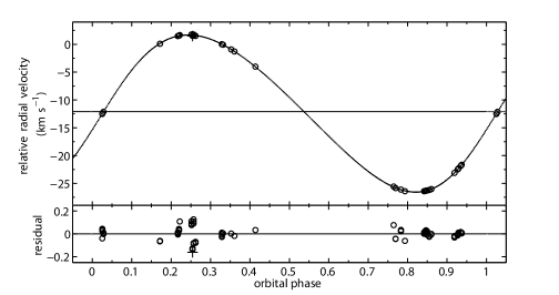
(a) Phase plot of HD 194215 radial velocities.

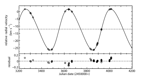
(b) Measured radial velocities of HD 194215 versus Julian date.

Figure 7: Radial velocities of HD 194215 measured from the Hercules spectra. The plotted curves are calculated from the orbital solution calculated from these radial velocities. The second panels show the residuals from this fit.

6 The reality of small detected eccentricities

In this section we analyse the reality of the small eccentricities found for the 12 stars discussed in this paper and by Komonjinda et al. (2011). The tests used are those described by Lucy (2005) and also by Lucy & Sweeney (1971).

The first Lucy test calculates the probability ($p_{1}$) that the star really has a circular orbit, but by chance the data show a small eccentricity, shown by a second harmonic in the velocity curve. If $p_{1}<0.05$, the eccentricity found is deemed to be significant.

However, the possibility remains that the second harmonic may be caused by a non-keplerian perturbation. If the data indicate a keplerian eccentric orbit, then the third harmonic must have the amplitude and phase which are consistent with the observed second harmonic. As pointed out by Lucy (2005), the components of the keplerian third harmonic are $C_{3}\cos 3L=\frac{9}{8}Ke^{2}\cos 2\omega\cos 3L$ and $S_{3}\sin 3L=\frac{9}{8}Ke^{2}\sin 2\omega\sin 3L$, where $L=2\pi(t-T)/P+\omega$ is the mean longitude. These compare with the generally much larger keplerian second harmonic components of $C_{2}\cos 2L=Ke\cos\omega\cos 2L$ and $S_{2}\sin 2L=Ke\sin\omega\sin 2L$.

The second Lucy test is to add a non-keplerian third harmonic perturbation to the eccentric keplerian orbit $V_{\rm K}$ so that the observed velocities become $V_{\rm obs}=V_{\rm K}+\Delta C_{3}\cos 3L+\Delta S_{3}\sin 3L$. The observed estimate of the amplitude of the non-keplerian perturbation is designated as $\delta_{3}=(\delta C_{3},\delta S_{3})$. The probability $p_{2}$ measures the probability that the data indicate a perturbation by chance, even though a purely keplerian eccentric orbit is being followed. If $p_{2}<0.05$, then the perturbation is deemed to be real; a larger value indicates a keplerian orbit.

Lucy (2005) has proposed two further tests. The third is to find the probability ($q_{1}$) that no keplerian third harmonic has been detected, and the fourth is to find the probability ($q_{2}$) that no third harmonic, whether keplerian or from a perturbation, has been detected. Lucy defines the parameter $p_{3}$ as the larger of $q_{1}$ and $q_{2}$ and uses the parameters $p_{2},p_{3}$ to divide the stars into four classes:

class A

$p_{2}>0.05;p_{3}<0.05$ An unperturbed keplerian eccentric orbit is strongly supported.

class B

$p_{2}<0.05;p_{3}<0.05$ An eccentric orbit has some support. However, a perturbation is detected, so the orbital elements are in doubt.

class C

$p_{2}>0.05;p_{3}>0.05$ The eccentricity is not strongly supported. Although no perturbation in the third harmonic is detected, no keplerian third harmonic is detected either. The second harmonic may arise from a perturbation or a small eccentricity.

class D

$p_{2}<0.05;p_{3}>0.05$ An eccentric keplerian orbit is in doubt. The keplerian third harmonic is not detected, but a third harmonic arising from a perturbation is detected, as shown by its amplitude and phase.

The results of all these tests are shown in Table 10. In this table the probabilities in column 2 are defined by Lucy (2005). In column 3, ($C_{2},S_{2}$) are the components of the second harmonic derived from a keplerian fit. In column 4, ($\delta C_{3},\delta S_{3}$) are the amplitudes of the orthogonal components of the non-keplerian perturbation obtained from our Hercules data. Column 5 gives the expected keplerian third harmonic amplitude calculated from our orbital elements. The eccentricity (possibly spurious) from a fitted keplerian orbit is in column 6. The last column is self-explanatory.

In summary, the results are as follows: four stars (HD 22905, HD 38099, HD 85622 and HD 101379) show $p_{1}>0.05$ so for these there is no reason to invoke a non-circular orbit. We conclude that the small eccentricities reported in the earlier literature are spurious. Nevertheless, for completeness, we have applied all the Lucy tests to all the stars, as even for these stars, a perturbation third harmonic could in principle be detected.

Table 10: The results of harmonic analysis of the velocity data using tests by Lucy.

Star	Probabilities	$(C_{2},S_{2})$	$(\delta C_{3},\delta S_{3}$)	$(C_{3},S_{3})$	$e$	Lucy
	$p_{1},p_{2},q_{1},q_{2},p_{3}$	ms-1	ms-1	ms-1		class
HD 352	$p_{1}=9.953e-29$	$C_{2}=-163.90$	$\delta C_{3}=-11.29\pm 15.07$	$C_{3}=-6.71$	$0.023$	D
	$p_{2}=1.555e-04$	$S_{2}=693.36$	$\delta S_{3}=-66.04\pm 15.67$	$S_{3}=-13.76$	$\pm 0.0006$
	$q_{1}=5.444e-01$
	$q_{2}=4.233e-06$
	$p_{3}=5.444e-01$
HD 9053	$p1=1.348e-44$	$C_{2}=-179.29$	$\delta C_{3}=-25.59\pm 13.41$	$C_{3}=1.09$	0.0301	C
	$p_{2}=1.048e-01$	$S_{2}=323.45$	$\delta S_{3}=1.03\pm 19.59$	$S_{3}=-16.65$	$\pm 0.0012$
	$q_{1}=6.151e-01$
	$q_{2}=1.936e-01$
	$p_{3}=6.151e-01$
HD 22905	$p_{1}=1.690e-01$	$C_{2}=-9.51$	$\delta C_{3}=47.71\pm 12.85$	$C_{3}=-0.04$	0.0010	D
	$p_{2}=6.408e-04$	$S_{2}=272.40$	$\delta S_{3}=18.63\pm 12.55$	$S_{3}=0.05$	$\pm 0.0014$
	$q_{1}=1.000$
	$q_{2}=6.428e-04$
	$p_{3}=1.000$
HD 30021	$p_{1}=1.622e-03$	$C_{2}=33.39$	$\delta C_{3}=-15.47\pm 10.76$	$C_{3}=-0.05$	0.0015	C
	$p_{2}=3.353e-01$	$S_{2}=33.39$	$\delta S_{3}=-3.91\pm 12.95$	$S_{3}=0.08$	$\pm 0.0015$
	$q_{1}=1.000$
	$q_{2}=3.338e-01$
	$p_{3}=1.000$
HD 38099	$p_{1}=5.228e-01$	$C_{2}=-59.46$	$\delta C_{3}=-33.86\pm 48.76$	$C_{3}=-0.50$	0.0076	C
	$p_{2}=6.531e-01$	$S_{2}=14.83$	$\delta S_{3}=-46.73\pm 55.24$	$S_{3}=-0.29$	$\pm 0.0067$
	$q_{1}=9.999e-01$
	$q_{2}=6.481e-01$
	$p_{3}=9.999e-01$
HD 50337	$p_{1}=2.073e-31$	$C_{2}=6.29$	$\delta C_{3}=38.11\pm 5.20$	$C_{3}=-0.88$	0.0059	D
	$p_{2}=1.567e-10$	$S_{2}=105.86$	$\delta S_{3}=12.44\pm 5.12$	$S_{3}=0.30$	$\pm 0.0003$
	$q_{1}=9.839e-01$
	$q_{2}=2.979e-10$
	$p_{3}=9.839e-01$
HD 77258	$p_{1}=4.260e-04$	$C_{2}=-4.61$	$\delta C_{3}=-6.82\pm 2.54$	$C_{3}=-0.01$	0.0009	D
	$p_{2}=2.927e-02$	$S_{2}=16.08$	$\delta S_{3}=-0.32\pm 2.94$	$S_{3}=-0.01$	$\pm 0.0002$
	$q_{1}=1.000$
	$q_{2}=2.885e-02$
	$p_{3}=1.000$
HD 85622	$p_{1}=1.517e-01$	$C_{2}=-33.50$	$\delta C_{3}=16.91\pm 9.66$	$C_{3}=0.10$	0.0026	C
	$p_{2}=9.079e-02$	$S_{2}=-4.71$	$\delta S_{3}=-9.98\pm 8.68$	$S_{3}=0.02$	$\pm 0.0016$
	$q_{1}=9.999e-01$
	$q_{2}=8.949e-02$
	$p_{3}=9.999e-01$
HD 101379	$p_{1}=4.467e-01$	$C_{2}=-84.38$	$\delta C_{3}=-72.75\pm 72.68$	$C_{3}=-0.94$	0.012	D
	$p_{2}=4.998e-06$	$S_{2}=-129.94$	$\delta S_{3}=-360.61\pm 67.20$	$S_{3}=2.02$	$\pm 0.010$
	$q_{1}=9.994e-01$
	$q_{2}=5.587e-06$
	$p_{3}=9.994e-01$
HD 124425	$p_{1}=2.570e-02$	$C_{2}=27.59$	$\delta C_{3}=14.78\pm 20.54$	$C_{3}=-0.13$	0.0026	C
	$p_{2}=7.198e-01$	$S_{2}=-0.91$	$\delta S_{3}=7.89\pm 21.01$	$S_{3}=-0.15$	$\pm 0.0010$
	$q_{1}=1.000$
	$q_{2}=7.249e-01$
	$p_{3}=1.000$

Table 10: The results of harmonic analysis of the velocity data using tests by Lucy (cont.).

Star	Probabilities	$(C_{2},S_{2})$	$(\delta C_{3},\delta S_{3}$)	$(C_{3},S_{3})$	$e$	Lucy
	$p_{1},p_{2},q_{1},q_{2},p_{3}$	ms-1	ms-1	ms-1		class
HD 136905	$p_{1}=1.003e-03$	$C_{2}=283.82$	$\delta C_{3}=-319.42\pm 58.30$	$C_{3}=1.86$	0.0079	D
	$p_{2}=9.895e-07$	$S_{2}=120.47$	$\delta S_{3}=39.17\pm 46.91$	$S_{3}=1.98$	$\pm 0.0026$
	$q_{1}=9.990e-01$
	$q_{2}=1.026e-06$
	$p_{3}=9.990e-01$
HD 194215	$p_{1}=1.422e-113$	$C_{2}=-357.67$	$\delta C_{3}=0.58\pm 7.03$	$C_{3}=-220.98$	0.1233	A
	$p_{2}=9.850e-01$	$S_{2}=-1703.15$	$\delta S_{3}=-0.93\pm 6.43$	$S_{3}=97.18$	$\pm 0.0008$
	$q_{1}=3.326e-56$
	$q_{2}=4.754e-56$
	$p_{3}=4.754e-56$

We find one of the 12 stars, HD 194215, to be in class A. No perturbation is detected for this star, and a fairly large non-zero eccentricity ($e=0.1233\pm 0.0001$) is clearly present, even though Bopp et al. (1970) had earlier reported a smaller value ($e=0.06\pm 0.01$).

We find none of our stars to be in Lucy class B. Five are in class C, where neither a keplerian third harmonic nor a perturbation third harmonic is detected, and six are in class D, where no keplerian third harmonic is detected, but a perturbation third harmonic is clearly seen. We can conclude that all the class D stars are affected by non-keplerian perturbations and probably have circular orbits. It is also possible that the class C stars also have circular orbits. We note that the keplerian third harmonics are nearly all predicted to have very small amplitudes, of the order of 1 ms^-1 in most cases, except for HD 194215, where it is a large 241 ms^-1. It is not surprising therefore that the keplerian third harmonics have been undetectable (with one exception) using our data with a typical precision per observation of about 10 ms^-1 in the best cases. On the other hand, the observed non-keplerian perturbation amplitudes of the third harmonic are occasionally quite large; for example 67 ms^-1 for HD 352, 51 ms^-1 for HD 22905, 322 ms^-1 for HD 136905 and 368 ms^-1 for HD 101379. Details are in Table 10. In all these cases, our data are readily able to detect such third harmonic perturbations.

For the Class D stars, as these are presumed to have circular orbits, the second harmonic must then arise entirely from non-keplerian effects, and this is commonly several hundred ms^-1. For the class C stars, the second harmonic may contain both keplerian and non-keplerian velocities.

7 Possible causes of non-keplerian velocity perturbations

It is interesting to consider the possible causes for non-keplerian perturbations. The most likely cause, originally suggested by Struve (1950), is starspots on a rotating star, which render the surface brightness of the visible hemisphere non-uniform and lead to rotational modulation of the observed radial velocity. Even for the Sun, which has an equatorial rotational velocity of about 2 km s^-1, a small number of starspots can easily perturb the mean velocity that would be observed for the visible hemisphere by several ms^-1. Given that our stars are giants and typically ten times larger than the Sun in radius, this magnifies the susceptibility of spots to perturb the observed radial velocity (for a given rotation period). Moreover, several stars in our list are known to be chromospherically active (HD 9053, HD 50337, HD 136905, HD 101379), so these probably have starspots.

We also note that another star ($\zeta$ TrA) that we had earlier analysed, also showed a small eccentricity ($e=0.0140\pm 0.0002$) (Skuljan et al., 2004) from our Hercules data. This star was subsequently shown by Lucy (2005) to be in class D, that is with no significant keplerian third harmonic but a significant perturbation third harmonic. We subsequently did tests with the Wilson-Devinney code (Wilson & Devinney, 1971) to model the effect of starspots on the observed radial velocity curve assuming a truly circular orbit. It was a simple matter to obtain spurious eccentricities comparable to those observed for $\zeta$ TrA by assuming a co-rotating model with a group of spots at about the same longitude and near the equator covering 12 per cent of the surface and with $\Delta T\sim 1000$ K (Komonjinda et al., 2006), or alternatively by adopting a model with two groups of spots each covering 8 per cent of the star’s surface area. For the class C and D stars in this paper and in Komonjinda et al. (2011) the eccentricities found range up to $e=0.03$ for HD 9053, but the values are mainly less than $e=0.01$, so we presume that spots can rather easily perturb the radial-velocity data to produce spurious eccentricities of this order.

Another possibility is that non-spherical tidally distorted stars with significant gravity darkening can also, as a result of their variation in surface brightness over the visible part of the surface, contribute to velocity perturbations, as discussed in some detail by Sterne (1941a). We consider this less likely for our sample of stars, because they mainly have orbital periods of several months to a year. Only HD 124425 has an orbital period of less than 10 days and is therefore likely to be more affected by tidal distortion caused by the secondary star. But even here, this is a Lucy class C star for which no perturbation third harmonic was detected. However, two stars we have observed are known to show ellipsoidal light variations, notably HD 136905, and possibly also HD 38099.

A third possibility is that the underlying secondary star spectrum has distorted our measurements of the radial velocity of the primary of our SB1 systems. We have not attempted to model this effect, but note that our stars all have giant, or even supergiant, primaries. It is likely that a common situation is a G or K giant primary with an M dwarf secondary, possibly as much as ten magnitudes fainter, given the large preponderance of M dwarfs in stellar statistics. Nevertheless three of our stars are thought to have F dwarf secondaries (HD 352, HD 22905, HD 136905) and two to have A dwarf secondaries (HD 50337, HD 77258). We acknowledge that if the visual luminosity of the secondary just happens to lie at more than two but less than four magnitudes below the primary, then it might have a disturbing effect on the primary star’s velocity measurements. We expect that secondaries at less than two magnitudes below the primary would have been detected and the system would have been classified as SB2, while those at more than four magnitudes, which is probably the case for the great majority of our stars, would have been too faint to cause a problem, as the secondary star’s spectrum would be comparable to or less than the photon noise in the recorded spectrum. The secondary spectrum in principle has the possibility of perturbing the measured velocities for almost any method of measuring Doppler shifts, whether by cross-correlation or some other technique. The perturbation would depend not only on the magnitude difference of the two stars, but also on the spectral type and radial velocity difference.

Although any of these processes may be the source of non-keplerian velocities, starspots and chromospheric activity remain the most likely explanation, especially in view of the fact noted that the most chromospherically active stars in our sample have the largest velocity perturbations.

8 Conclusion

We have analysed the orbits of six single-lined spectroscopic binary systems with nearly circular orbits, using high precision radial-velocity data from the Hercules fibre-fed vacuum spectrograph at Mt John Observatory. We have paid especial attention to obtaining precise (i.e. small random errors) values of the eccentricity by fitting keplerian orbits by the least squares method to the data points.

We have combined the results of the orbital analyses in this paper with six further SB1 orbits analysed by Komonjinda et al. (2011).

Our results show that only for one star (HD 194215) is there a clear and unequivocal orbital eccentricity detected ($e=0.1233\pm 0.0001$). For four stars (HD 22905, HD 38099, HD 85622 and HD 101379) our analysis of the data show that a circular orbit is the preferred solution. For six stars we find clear evidence of small systematic perturbations in the measured radial velocities which have produced spurious values of the eccentricity. These spurious eccentricities are mainly below $e=0.01$, but in one case it is as high as $e=0.03$ (HD 9053) and in another case it is $e=0.02$ (HD 352). Our analysis also gives quantitative estimates of the perturbation in second and third harmonics; values as small as 10 m s^-1 can be detected, and values over 300 m s^-1 can occur in moderately active stars.

Our overall conclusion is therefore that no matter how precise or numerous the radial-velocity data may be, conventional methods of velocity determination, such as by cross-correlation, lead to unavoidable systematic errors in the velocities, which are not random but depend on the phase, and which may amount to a few tens of ms^-1 to a few hundreds of ms^-1 in some cases. Therefore it is likely that the great majority of late-type giant spectroscopic binary orbital eccentricities cannot be trusted to an accuracy of better than a few times 0.01 in $e$. The only way to overcome this problem would be much more careful modelling of effects such as starspots, taking into account their distribution on the stellar surface and effect on line profiles through Doppler imaging. Our analysis measures the non-keplerian harmonics of circularized orbits at the 10 ms^-1 level for the first time, and demonstrates that circularization even to better than $e=0.01$ has been achieved for many of the stars in our sample.

This project had at its inception the goal of investigating very small reported eccentricities ($e\leq 0.05$) using the best high quality spectra from a high-dispersion vacuum fibre-fed échelle spectrograph, and possibly further to investigate whether complete circularization had been achieved at the $e=0.01$ level. Instead we have found that unavoidable systematic effects have hampered that line of investigation, but nevertheless this has led to new results of interest on the ability of spectroscopic data to determine the orbital eccentricity in binary stars and to quantify non-keplerian velocity perturbations.

Table 11: Radial velocities of HD 77258 relative to the image recorded at JD2453741.1562.

HJD	$V_{\mathrm{rad}}$	HJD	$V_{\mathrm{rad}}$	HJD	$V_{\mathrm{rad}}$
(2400000+)	(km s-1)	(2400000+)	(km s-1)	(2400000+)	(km s-1)
53323.1328	35.627	53453.0742	9.326	53488.8359	29.199
53377.0820	6.599	53456.8085	15.153	53488.8398	29.202
53402.0781	37.863	53456.8125	15.151	53490.8632	26.250
53403.0703	37.915	53456.8164	15.183	53490.8671	26.241
53403.9609	37.615	53456.8203	15.180	53490.8710	26.238
53404.0234	37.691	53464.9531	28.236	53490.8750	26.231
53405.0429	37.637	53465.8750	29.512	53490.8789	26.223
53406.0898	37.304	53466.8710	30.847	53666.1562	$-$0.491
53424.9179	12.859	53486.8515	31.786	53666.1601	$-$0.484
53425.0312	12.695	53486.8554	31.782	53666.1640	$-$0.478
53451.9726	7.615	53486.8593	31.777	53689.1718	30.698
53451.9765	7.625	53486.8632	31.770	53689.1757	30.705
53452.9960	9.111	53488.8320	29.220	53721.1210	13.401
53453.0078	9.138	53488.8320	29.203	53721.1250	13.380
53741.1484	0.002	53835.9335	28.593	53885.8906	$-$1.333
53741.1523	$-$0.014	53835.9375	28.602	53885.9023	$-$1.354
53741.1562	0.000	53835.9414	28.611	53887.8242	$-$0.842
53742.0976	0.623	53835.9453	28.608	53887.8281	$-$0.838
53742.1015	0.624	53858.9179	30.040	53887.8320	$-$0.838
53742.1054	0.631	53858.9218	30.032	53887.8359	$-$0.838
53743.0507	1.379	53858.9296	30.028	53890.9257	1.042
53743.0585	1.379	53858.9335	30.032	53890.9335	1.059
53744.0859	2.350	53858.9375	30.029	53890.9375	1.050
53744.0898	2.347	53860.9375	27.166	53891.8789	1.864
53778.0976	36.220	53860.9375	27.156	53891.8828	1.890
53778.1015	36.197	53860.9414	27.141	53891.8867	1.899
53778.1093	36.201	53860.9453	27.142	53891.8906	1.909
53779.1445	35.600	53861.9375	25.635	53893.8125	3.864
53779.1484	35.609	53861.9414	25.637	53893.8125	3.873
53779.1523	35.626	53861.9453	25.628	53893.8203	3.872
53829.9492	19.223	53861.9492	25.622	53893.8203	3.876
53829.9531	19.233	53861.9531	25.622	53929.8046	33.769
53829.9570	19.232	53861.9531	25.615	53929.8125	33.866
53829.9609	19.243	53885.8828	$-$1.333

Table 12: Radial velocities of HD 85622 relative to the image recorded at JD2453835.9726.

HJD	$V_{\mathrm{rad}}$	HJD	$V_{\mathrm{rad}}$	HJD	$V_{\mathrm{rad}}$
(2400000+)	(km s-1)	(2400000+)	(km s-1)	(2400000+)	(km s-1)
53323.1523	$-$20.257	53490.9101	$-$2.112	53860.9609	1.512
53377.0898	$-$24.424	53490.9140	$-$2.119	53860.9648	1.493
53402.0859	$-$21.613	53490.9179	$-$2.090	53860.9687	1.493
53403.0781	$-$21.518	53490.9257	$-$2.098	53860.9726	1.497
53403.9687	$-$21.634	53692.1718	$-$24.592	53861.9804	1.484
53404.0351	$-$24.270	53692.1718	$-$24.592	53861.9843	1.500
53405.0507	$-$21.159	53741.1640	$-$19.888	53861.9882	1.498
53406.0976	$-$21.044	53741.1679	$-$19.882	53861.9882	1.502
53424.9375	$-$17.486	53741.1718	$-$19.875	53885.9101	$-$0.122
53425.0507	$-$17.526	53742.1132	$-$19.763	53885.9179	$-$0.135
53451.9843	$-$10.755	53742.1210	$-$19.770	53885.9218	$-$0.128
53451.9921	$-$10.747	53742.1289	$-$19.760	53885.9257	$-$0.123
53451.9960	$-$10.738	53744.0976	$-$19.312	53887.8437	$-$0.188
53456.9765	$-$9.511	53744.1054	$-$19.319	53887.8476	$-$0.201
53456.9804	$-$9.512	53778.1132	$-$12.055	53887.8515	$-$0.214
53456.9843	$-$9.500	53778.1210	$-$12.061	53887.8554	$-$0.222
53456.9882	$-$9.511	53778.1289	$-$11.999	53890.9687	$-$0.736
53465.9062	$-$7.308	53835.9726	0.000	53890.9765	$-$0.741
53466.9140	$-$7.111	53835.9804	0.008	53890.9843	$-$0.737
53486.8945	$-$2.785	53835.9843	0.006	53891.8945	$-$0.787
53486.8984	$-$2.783	53835.9882	0.001	53891.9023	$-$0.801
53486.9023	$-$2.783	53835.9960	$-$0.004	53891.9062	$-$0.807
53486.9023	$-$2.785	53858.9765	1.585	53893.8437	$-$1.116
53488.8476	$-$2.498	53858.9843	1.591	53893.8515	$-$1.124
53488.8515	$-$2.493	53858.9882	1.591	53893.8554	$-$1.139
53488.8554	$-$2.490	53860.9531	1.497	53893.8554	$-$1.127
53488.8593	$-$2.506	53860.9570	1.516	53894.8007	$-$1.250
53894.8046	$-$1.243	53894.8125	$-$1.230	53929.8242	$-$8.277
53894.8085	$-$1.234	53928.8359	$-$8.079

Table 13: Absolute radial velocities of HD 101379 obtained using HD 109379 (G5II) as a standard star.

HJD	$V_{\mathrm{rad}}$	HJD	$V_{\mathrm{rad}}$	HJD	$V_{\mathrm{rad}}$
(2400000+)	(km s-1)	(2400000+)	(km s-1)	(2400000+)	(km s-1)
53304.1054	14.893	53465.0117	$-$9.838	53779.1796	$-$3.842
53322.1640	1.617	53465.9375	$-$9.242	53779.1875	$-$3.807
53377.1289	9.489	53466.9531	$-$8.476	53836.0039	$-$8.143
53402.1015	$-$10.464	53486.9687	13.368	53859.0000	13.280
53402.1757	$-$10.508	53486.9765	13.367	53859.0117	13.271
53403.0859	$-$10.000	53486.9804	13.350	53859.0234	13.275
53403.1445	$-$10.035	53488.0039	13.865	53859.9687	13.207
53404.0156	$-$9.589	53488.0117	13.868	53859.9804	13.203
53404.0859	$-$9.557	53488.0234	13.867	53859.9960	13.196
53404.1367	$-$9.470	53488.9179	14.132	53861.0039	13.016
53405.0585	$-$8.634	53488.9257	14.133	53861.0078	13.031
53405.1367	$-$8.587	53488.9335	14.111	53861.0156	13.059
53406.0156	$-$7.674	53490.9335	14.324	53861.0234	13.026
53406.1210	$-$7.669	53490.9414	14.322	53862.0273	12.738
53423.9296	12.500	53490.9492	14.354	53862.0312	12.739
53423.9609	12.524	53742.1679	11.287	53862.0390	12.729
53424.9687	13.115	53744.1367	9.605	53862.0468	12.732
53457.0312	$-$10.842	53744.1445	9.574	53885.9648	$-$11.554
53457.0429	$-$10.852	53779.1757	$-$3.856	53885.9726	$-$11.570
53885.9804	$-$11.571	53891.9570	$-$11.724	53894.8906	$-$10.226
53885.9882	$-$11.571	53891.9648	$-$11.721	53894.8945	$-$10.234
53887.8828	$-$12.165	53891.9726	$-$11.730	53927.8320	9.865
53887.8906	$-$12.175	53893.8867	$-$10.885	53929.8398	7.896
53887.8945	$-$12.177	53893.8906	$-$10.873	53929.8515	7.895
53891.0000	$-$12.066	53893.8945	$-$10.883
53891.0117	$-$12.066	53894.8828	$-$10.259

Table 14: Radial velocities of HD 124425 relative to the image recorded at JD2453405.1757.

HJD	$V_{\mathrm{rad}}$	HJD	$V_{\mathrm{rad}}$	HJD	$V_{\mathrm{rad}}$
(2400000+)	(km s-1)	(2400000+)	(km s-1)	(2400000+)	(km s-1)
53402.1640	7.174	53487.0234	40.302	53861.9648	42.839
53404.1679	44.936	53488.9726	1.966	53862.0859	48.013
53405.1640	0.053	53488.9804	2.169	53862.0976	48.259
53405.1757	0.000	53488.9921	2.576	53886.0039	29.925
53406.1718	42.776	53490.9609	17.779	53886.0117	30.520
53452.0468	44.058	53490.9726	17.187	53887.9375	0.072
53452.0625	44.730	53490.9882	16.359	53887.9492	0.103
53453.1171	22.795	53778.1835	32.932	53887.9570	0.016
53453.1328	21.890	53836.1601	19.109	53890.9531	5.842
53456.0937	7.922	53837.0898	8.994	53891.9140	51.517
53456.1054	7.464	53837.1054	9.734	53892.0195	52.208
53456.1132	7.077	53859.0742	32.515	53893.8359	14.350
53457.0585	22.815	53859.0859	33.257	53893.9062	18.418
53457.0664	23.287	53860.0156	42.659	53894.0234	25.747
53465.0546	17.497	53860.0234	42.385	53894.0351	26.312
53466.0195	50.710	53860.9179	0.289	53894.0429	26.808
53467.0429	2.357	53860.9257	0.187	53894.7890	51.807
53487.0039	39.207	53861.0312	0.083	53894.8476	50.718
53487.0156	39.737	53861.0390	0.036	53894.8593	50.569
53894.8710	50.161	53895.0234	45.232	53929.8789	51.087
53894.9414	48.181	53927.8437	20.216
53895.0117	45.699	53929.8632	51.420

Table 15: Radial velocities of HD 136905 relative to the image recorded at JD2453452.105.

HJD	$V_{\mathrm{rad}}$	HJD	$V_{\mathrm{rad}}$	HJD	$V_{\mathrm{rad}}$
(2400000+)	(km s-1)	(2400000+)	(km s-1)	(2400000+)	(km s-1)
53452.105	0.000	53859.125	$-$32.892	53886.043	$-$6.659
53465.082	27.549	53860.043	$-$45.228	53886.059	$-$6.344
53466.039	27.124	53860.059	$-$45.379	53887.973	26.000
53487.047	25.289	53860.078	$-$45.519	53887.984	26.078
53487.059	25.510	53860.094	$-$45.646	53888.000	26.227
53487.074	25.598	53861.094	$-$48.222	53888.012	26.314
53487.090	25.709	53861.105	$-$48.221	53892.035	$-$23.436
53487.109	25.846	53861.117	$-$48.171	53892.051	$-$23.800
53488.070	28.160	53861.129	$-$48.129	53893.922	$-$48.124
53489.070	20.775	53862.109	$-$39.495	53893.934	$-$48.146
53489.090	20.527	53862.125	$-$39.336	53893.949	$-$48.200
53491.008	$-$19.096	53862.137	$-$39.161	53894.961	$-$45.697
53491.027	$-$19.506	53862.152	$-$38.919	53894.973	$-$45.582
53859.109	$-$32.577	53886.027	$-$6.954	53927.883	$-$48.384

Table 16: Radial velocities of HD 194215 relative to the image recorded at JD2453666.8515.

HJD	$V_{\mathrm{rad}}$	HJD	$V_{\mathrm{rad}}$	HJD	$V_{\mathrm{rad}}$
(2400000+)	(km s-1)	(2400000+)	(km s-1)	(2400000+)	(km s-1)
53251.9062	1.647	53666.8398	0.004	53888.0976	$-$23.126
53300.8750	$-$0.920	53666.8515	0.000	53888.1093	$-$23.127
53303.8984	$-$1.299	53666.8593	$-$0.004	53888.1210	$-$23.113
53323.8671	$-$4.016	53666.9257	0.010	53888.1289	$-$23.121
53457.2148	$-$25.832	53666.9414	0.025	53888.1367	$-$23.119
53457.2265	$-$25.836	53667.9257	$-$0.077	53888.1484	$-$23.119
53457.2382	$-$25.837	53830.2382	$-$25.566	53891.1914	$-$22.494
53457.2460	$-$25.836	53837.1914	$-$26.104	53891.2031	$-$22.487
53466.1562	$-$26.392	53837.2070	$-$26.112	53891.2187	$-$22.487
53489.2148	$-$26.179	53837.2187	$-$26.111	53891.2343	$-$22.475
53489.2304	$-$26.185	53837.2343	$-$26.102	53891.9843	$-$22.310
53489.2421	$-$26.184	53859.2109	$-$26.405	53891.9960	$-$22.303
53491.2109	$-$26.029	53859.2187	$-$26.402	53892.0039	$-$22.300
53491.2226	$-$26.028	53859.2265	$-$26.400	53894.1093	$-$21.846
53491.2304	$-$26.023	53859.2343	$-$26.407	53894.1171	$-$21.839
53607.8906	0.083	53859.2421	$-$26.394	53894.1250	$-$21.840
53607.9023	0.087	53859.2539	$-$26.395	53894.1328	$-$21.840
53608.0117	0.099	53860.2109	$-$26.344	53895.0390	$-$21.640
53608.0195	0.102	53860.2226	$-$26.351	53895.0507	$-$21.642
53638.9843	1.517	53860.2304	$-$26.346	53928.0000	$-$12.513
53638.9921	1.507	53860.2382	$-$26.343	53928.0117	$-$12.426
53639.0000	1.483	53861.0546	$-$26.298	53928.0195	$-$12.442
53639.9101	1.544	53861.0625	$-$26.323	53928.0312	$-$12.428
53639.9218	1.548	53861.0742	$-$26.321	53929.0820	$-$12.134
53641.8085	1.518	53861.0820	$-$26.327	53929.0937	$-$12.133
53641.8203	1.520	53862.0585	$-$26.256	53929.1054	$-$12.139
53641.8281	1.511	53862.0664	$-$26.287	53999.8320	1.476
53999.8476	1.479	54000.9101	1.548	54012.8867	1.733
53999.8671	1.488	54000.9257	1.557	54014.8085	1.720
53999.8867	1.489	54000.9375	1.555	54014.8203	1.735
53999.9023	1.485	54000.9492	1.544	54014.8242	1.755
53999.9179	1.471	54012.8632	1.767
53999.9335	1.478	54012.8750	1.744

References

- Balona (1987) Balona, L.A., 1987, SAAO Circ., 11, 1
- Bidelman & MacConnell (1973) Bidelman, W.P. & MacConnell, D.J., 1973, AJ, 78, 687
- Bopp et al. (1970) Bopp, B.W., Evans, D.S., Laing, J.D. & Deeming, T.J., 1970, MNRAS, 147, 355
- Burke et al. (1982) Burke, E.W., Baker, J.E., Fekel, F.C., Hall, D.S. & Henry, G.W., 1982, IBVS, 2111, 1
- Buscombe (1962) Buscombe, W., 1962, Mt Stromlo Observ. Mimeo., 4, 1
- Buscombe & Morris (1958) Buscombe, W. & Morris, P.M., 1958, MNRAS, 118, 609
- Collier (1982) Collier, A.C., 1982, PhD thesis, University of Canterbury, NZ
- Collier et al. (1982) Collier, A.C., Haynes, R.F., Slee, O.B., Wright, A.E. & Hillier, D.J., 1982, MNRAS, 200, 869
- Collier Cameron (1987) Collier Cameron, A., 1987, SAAO Circ., 11, 13
- de Medeiros et al. (2002) de Medeiros, J.R., Udry, S., Burki, G. & Mayor, M., 2002, A&A, 395, 97
- de Vaucouleurs (1957) de Vaucouleurs, A., 1957, MNRAS, 117, 449
- Duncan (1921) Duncan, J.C., 1921, ApJ, 54, 226
- Fekel et al. (1985) Fekel, F.C., Hall, D.S., Africano, J.L., Gillies, K., Quigley, R. & Fried, R.E., 1985, AJ, 90, 2581
- Hearnshaw et al. (2002) Hearnshaw, J.B., Barnes, S.I., Kershaw, G.M., Frost, N., Graham, G., Ritchie, R. & Nankivell, G.R., 2002, Exper. Astron., 13, 59
- Houk & Cowley (1975) Houk, N. & Cowley, A.P., 1975, Michigan Catalogue of two-dimensional spectral types for the HD stars, Univ. of Michigan, Ann Arbor
- Houk (1982) Houk, N., 1982, Michigan Catalogue of two-dimensional spectral types for the HD stars, vol. 3, Univ. of Michigan, Ann Arbor
- Jones (1928) Jones, H.S., 1928, Ann. Cape Observ., 10, 1
- Kaye et al. (1995) Kaye, A.B., Hall, D.S., Henry, G.W., Eaton, J.A., Lines, R.D., Lines, H.C., Barksdale, W.S., Beck, S.J., Chambliss, C.R., Fried, R.E., Genet, R.M., Hopkins, J.L., Lovell, L.P., Louth, H.P., Montle, R.E., Renner, T.R. & Stelzer, H.J., 1995, AJ, 109, 2177
- Komonjinda et al. (2006) Komonjinda, S., Hearnshaw, J.B. & Ramm, D.J., 2006, IAU Symp. 240, 531
- Komonjinda et al. (2011) Komonjinda, S., Hearnshaw, J.B. & Ramm, D.J., 2011, MNRAS, 410, 1761
- Lehmann-Filhés (1894) Lehmann-Filhés, R., 1894, AN, 136, 17
- Lucy (2005) Lucy, L.B., 2005, A&A, 439, 663
- Lucy & Sweeney (1971) Lucy, L.B. & Sweeney, M.A., 1971, AJ, 76, 544
- Lunt (1919) Lunt, J., 1919, ApJ, 50, 161
- Lunt (1924) Lunt, J., 1924, Ann. Cape Observ., 10, 1
- Luyten (1936) Luyten, W.J., 1936, ApJ, 84, 85
- MacConnell & Bidelman (1976) MacConnell, D.J. & Bidelman, W.P., 1976, AJ, 81, 225
- MacQueen (1986) MacQueen, P.J., 1986, PhD thesis, Univ. Canterbury, NZ
- Mayor & Mazeh (1987) Mayor, M. & Mazeh, T., 1987, A&A, 171, 157
- McAlister et al. (1990) McAlister, H.A., Hartkopf, W.I. & Franz, O.G., 1990, AJ, 99, 965
- Monet (1979) Monet, D.G., 1979, PASP, 91, 95
- Murdoch et al. (1995) Murdoch, K.A., Hearnshaw, J.B., Kilmartin, P.M. & Gilmore, A.C., 1995, MNRAS, 276, 836
- Pourbaix et al. (2004) Pourbaix, D., Tokovinin, A.A., Batten, A.H., Fekel, F.C., Hartkopf. W.I., Levato, H., Morrell, N.I., Torres, G. & Udry, S., 2004, A&A, 424, 727
- Ramm (2004) Ramm, D.J., 2004, unpubl. PhD thesis, Univ. of Canterbury, N.Z.
- Simkin (1974) Simkin S.M., 1974, A&A, 31, 129
- Skuljan (2003) Skuljan, J., 2003, The Hercules Reduction Software Package HRSP ver 2.3, unpublished software and manual, Dept. of Physics and Astronomy, Univ. of Canterbury
- Skuljan et al. (2004) Skuljan, J., Ramm, D.J. & Hearnshaw, J.B., 2004, MNRAS, 352, 975
- Sterne (1941a) Sterne, T.E., 1941a, Proc. Nat. Acad. Sci., 27, 168
- Sterne (1941b) Sterne, T.E., 1941b, Proc. Nat. Acad. Sci., 27, 175
- Struve (1950) Struve, O., 1950, Pop. Astron., 58, 7
- Wilson & Devinney (1971) Wilson, R.E. & Devinney, E.J., 1971, ApJ, 166, 605
- Wright (1904) Wright, W.H., 1904, Lick Observ. Bull., 60, 3 (see also ApJ, 20, 140)
- Wright (1907) Wright, W.H., 1907, ApJ, 25, 56
- (44)