Probing the bias of radio sources at high redshift

Abstract

The relationship between the clustering of dark matter and that of luminous matter is often described using the bias parameter. Here, we provide a new method to probe the bias of intermediate to high-redshift radio continuum sources for which no redshift information is available. We matched radio sources from the Faint Images of the Radio Sky at Twenty centimetres (FIRST) survey data to their optical counterparts in the Sloan Digital Sky Survey (SDSS) to obtain photometric redshifts for the matched radio sources. We then use the publicly available semi-empirical simulation of extragalactic radio continuum sources (S³) to infer the redshift distribution for all FIRST sources and estimate the redshift distribution of unmatched sources by subtracting the matched distribution from the distribution of all sources. We infer that the majority of unmatched sources are at higher redshifts than the optically matched sources and demonstrate how the angular scales of the angular two-point correlation function can be used to probe different redshift ranges. We compare the angular clustering of radio sources with that expected for dark matter and estimate the bias of different samples.

1 Introduction

Current and future radio continuum surveys typically probe redshifts out to $z\sim 5$ and often cover a significant fraction of the sky. The large volumes accessible in these surveys provide a probe of the large-scale structure and thus can be utilised to test cosmological models. One of the most common approaches to investigate the large-scale distribution of cosmological objects is the two-point angular correlation function (ACF) which quantifies the projected clustering of galaxies on the plane of the sky. To gain information on the three dimensional distribution of galaxies and their evolution with time, the redshift distribution of the sample needs to be known. However, in general, redshifts can not be obtained from radio continuum surveys since the spectra do not show emission or absorption line features. One way to gain redshift information of these radio sources is to match them to their optical counterparts for which the redshifts are known.

First attempts to detect clustering in radio surveys were carried out in the 1970s, but it was only in 1996 (Cress et al., 1996) that the first high-significance detection of the clustering was made using the Faint Images of the Radio Sky at Twenty centimetres (FIRST) survey (Becker et al., ). They found that on angular scales that probe large-scale structure, the ACF of galaxies detected down to 1 mJy at 1.4 GHz is well-represented by a power-law, with a slope somewhat steeper than that found for typical optical surveys. A number of other studies, e.g Overzier et al. (2003) and Blake and Wall (2002) also measured clustering of radio sources using the ACF in the FIRST survey, in the NRAO VLA Sky Survey (NVSS, Condon et al. 1998) and in the Westerbork Northern Sky Survey (WENSS, Rengelink et al. 1997). Whilst there was some disagreement about the slope of the correlation function on larger angular scales, later work by Blake et al. (2004) highlighted problems with their earlier results (associated with over-cleaning of potential sidelobe sources) and obtained results from all the surveys consistent with Cress et al. (1996).

In essence, all these studies are confined to the investigation of the projected clustering signal, since many of the sources are too faint in the optical/IR to obtain accurate redshifts. However, some information on real-space clustering can be inferred, but this relies on estimates of the average redshift distributions of the sources.

During the 1990s, Dunlop and Peacock (1990) developed models to infer the redshift distribution of faint radio sources extrapolating from data at much higher flux densities. Since then, a number of observations have improved our knowledge in this area. Waddington et al. (2001) estimated redshifts of a complete sample of 72 radio galaxies down to 1 mJy in about one square degree (65% with spectroscopic redshifts). In the Combined EIS-NVSS Survey Of Radio Sources (CENSORS, Best et al. 2003; Brookes et al. 2006, 2008), redshifts were estimated for 150 sources, in a 6 square degree region, with flux densities above 7.2 mJy in NVSS (63% of them secure spectroscopic redshifts). Magliocchetti et al. (2004) studied the optical matches of FIRST sources in the 2dF survey (Colless et al., ) and Mauch and Sadler (2007) studied NVSS matches with $K<12.75$ mag in the 6dF survey (Wakamatsu et al., ). These studies all confirmed the picture that mJy-radio surveys contain a heterogenous population of galaxies that is dominated by AGN at higher flux densities and includes significant fractions of fainter star-forming galaxies at lower redshifts. They also appeared to rule out a large ‘spike’ of very low-z objects predicted by some of the Dunlop and Peacock models.

Understanding the nature of the sources in the radio surveys contributes to our knowledge of the $bias$ of the sources i.e. the clustering strength of the sources relative to clustering strength of the underlying dark matter. Knowing the bias is essential for using clustering as a cosmological probe as it enters into measurements of autocorrelations, the Integrated-Sachs Wolf (ISW) effect and the lensing effect. However, little is known about the bias of radio sources. Cress and Kamionkowski (1998) presented estimates of the bias based on the FIRST sources. Since then, different and sometimes contradictory prescriptions for the bias of radio sources have been used (e.g., Raccanelli et al., 2008; Raccanelli, 2011). Wilman et al. (2010) utilised a semi-empirical approach with a bias prescription based on the work of Mo and White (1996) to predict the clustering of radio sources in future radio surveys. The bias value in these models is artificially kept from rising to “non-physical” levels which underscores the lack of understanding of the bias of radio sources.

Future radio surveys carried out by the Square Kilometre Array (SKA) will potentially reach 1 nJy, providing catalogs of sources over 3$\pi$ of the sky. SKA Pathfinders such as the LOw Frequency ARray (LOFAR), the Australian Square Kilometre Array Pathfinder (ASKAP), the South African Karoo Array Telescope (MeerKAT), the Westerbork Synthesis Radio Telescope (WSRT) using the Apertif instrument and the extended Very Large Array (eVLA) will soon provide surveys with unprecedented depth and/or sensitivity. The resulting radio auto-correlations and cross-correlations with other datasets such as the CMB can provide valuable tests of cosmology. They can shed light on the question of non-gaussian initial conditions in the universe (Xia et al., 2010) and on issues concerning Dark Energy via the ISW effect (e.g. Nolta et al., 2004; Raccanelli et al., 2008). They may also provide strong tests of modified gravity (e.g. Raccanelli, 2011) and be used as direct probe of dark matter through gravitational lensing effects (e.g. Carilli and Rawlings, 2004; Kamionkowski et al., 1998; Raccanelli, 2011). It is essential for these studies to have a good understanding of the underlying bias of radio galaxies. In recent studies, (e.g. Raccanelli, 2011), predictions for future constraints on cosmology have been made by marginalizing over a single bias parameter but this does not capture the uncertainties in the evolution of bias which could be very important for the interpretation of measurements.

Therefore, in this article we attempt to make a direct measurement of the bias of FIRST radio sources at intermediate redshifts. We match FIRST sources to galaxies in the Sloan Digital Sky Survey Data Release 7 (SDSS-DR7, e.g. Abazajian et al. 2009 )and determine the redshift distribution of the matched sources. We then create a catalog of unmatched sources to probe the higher-z population.

The format of the paper is as follows. In § 2 we discuss the data and our methodology; in § 3 we discuss the results and present an estimate of the bias of radio sources at high redshift. Finally, in § 4 present our conclusions.

2 Data and methodology

Our approach to isolating a high-z sample of FIRST sources and estimating its redshift distribution can be summarised in the following steps:

1. Match the FIRST sources to galaxies from the SDSS survey and establish the redshift distribution of the matches from an SDSS photometric redshift catalogue

2. Use the S³ simulations (Wilman et al., 2010) to estimate an average redshift distribution for all FIRST sources.

3. Estimate the redshift distribution of unmatched sources by removing the matched distribution from the distribution of all sources. It is then inferred that the unmatched sources are mostly at higher redshifts.

4. The angular clustering of the high-z sample can then be measured and compared with what is expected for Dark Matter sampling the same redshift range, to obtain an estimate of the bias.

2.1 Creating the catalogues

2.1.1 The FIRST survey selection

In this section we describe the sample selection of the radio sources. Table 1 summarises our selection criteria quoted below. The FIRST survey mapped a region of the sky covering 10,000 ${\rm deg}^{2}$ in the Northern Galactic Cap at 1.4 GHz down to 1.4 mJy. The final catalogue contained a total of 816,331 sources with a completeness of 95% down the lower flux level used of 2 mJy.

Creating our sample of FIRST sources to be matched to SDSS required various steps to minimise potential sources of contamination. In the first step, we removed objects with a high probability of being a sidelobe. The FIRST survey has assigned to each source a probability of being a sidelobe ranging from 0 (indicating an object is not a sidelobe) to 1.0 (indicating an object is a sidelobe). To reduce this source of contamination, we explored various sidelobe probability values on our initial clustering analysis. This is discussed in more detail in § 3. However, we note that for our final selection we found a sidelobe probability value of 0.7 led to results the had minimal effects from the presents for sidelobes or the over-cleaning of them . For a sidelobe probability of 0.7 we were left with 795,453 sources.

The next step required the collapsing of multiple components (e.g. double lobes) to a single source. Following Cress et al. (1996) we chose a collapsing radius of 72”. This is the linking length of the friends-of-friends algorithm the we use to generate the groups of sources. We found that the average collapsed group had 2 to 3 components and a few groups that had up to 20 components. To compute the flux for each collapsed source, the integrated flux of each component was added together. The flux-weighted average positions were then calculated and used to match with the SDSS. This collapsing radius reduced the sample to 647,985 sources.

Table 1: Detailing the number of sources that satisfy our source collapsing, area selection and minimum flux cuts.

Radio sample	Numbers
Total FIRST	816,331
No. of sources after side-lobe removal	795,453
Collapsing sources in groups $<$ 72”	253,971
collapsed sources	106,503
single sources	541,482
No. of sources after collapsing	647,985
No. of sources in selected area
(130 $\leq$ RA $\leq$ 240, 5 $\leq$ Dec $\leq$ 55)	307,859
No. of sources $\geq$ 2 mJy	219,060

Furthermore we only take into account sources within a region that avoided both gaps in data and the edges of the SDSS and FIRST surveys. This region is defined by, 130 $\leq$ RA $\leq$ 240, 5 $\leq$ Dec $\leq$ 55, covering a total area of 4613.43 ${\rm deg}^{2}$. Our final catalogue of FIRST sources to be matched with SDSS contained a total of 307,859 objects.

Finally, in an attempt to minimize effects due to fluctuations in sensitivity noted in Blake et al. 2004 we applied a 2 mJy flux cut which is more than $10$ times the RMS fluctuations in the considered region. This leaves us with 219,060 sources.

In an attempt to isolate the AGN in the sample and exclude most of the low-z star-forming galaxies, we consider a sample containing only sources with flux densities greater than 7 mJy Waddington et al. (2001) this also allows us to compare the redshift distribution to the CENSORS survey. This leaves us with 93,202 sources in the 7 mJy subsample.

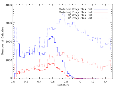
Figure 1: The photometric redshift distributions of the 2 mJy (blue) & 7 mJy (red) flux cuts of the FIRST sources that have been matched to the SDSS photometric survey (solid lines). The S³ redshift distributions for the same cuts are shown as dashed lines. The distributions correspond a sky coverage of 4613.43 ${\rm deg}^{2}$ and the S³ sample has been scaled accordingly to reflect this.

2.1.2 Matching to the SDSS galaxies

To match our FIRST sample to their optical counterpart we used data from the SDSS-DR7 (see e.g. Abazajian et al., 2009, for a description of the seventh data release). In broad terms, the SDSS has mapped a quarter of the entire sky with unprecedented accuracy using multi-band photometry ($u,g,r,i$ and $z$) from the 2.5-meter telescope on Apache Point to a limiting magnitude of $r<22.2$. The second phase of the project is now complete and is ideally suited to our studies as it is fully contained within the FIRST survey area.

The number density of SDSS-DR7 photometric sources is orders of magnitudes greater than the density of 2 mJy FIRST sources. The average size of SDSS galaxies is between 2” and 5s. To avoid erroneous matches we have chosen a relatively conservative matching radius of 2” to match our FIRST sample to the SDSS-DR7 photometric catalogue. To ensure accurate matches we only consider objects classified by the SDSS pipeline as a galaxy, requiring that they are successfully deblended to obtain precise positions, and have reliable photometric measurements in all 5 SDSS filters. Redshifts for the matched SDSS galaxies are taken from (Oyaizu et al., 2008). Specifically, we use the photometric redshift estimated from a Neural Network method inferred from the 4 galaxy colours and 3 concentration indices. This estimate is recommended for faint ($r>20$) galaxies, which dominate the matched galaxy sample. Finally, we apply a minimum redshift cut of $z>0.01$ to remove contamination from misidentified stars.

It should also be noted that we are likely to miss some of the optical identifications of fairly nearby multi-component radio sources as the collapsed source position may not give the position of the optical counterpart accurately enough. These sources are included in the redshift distribution of the simulations (but not in the matched redshift distribution) and thus will be included correctly in the unmatched redshift distribution. Our method for probing the average bias of the unmatched sample is thus still valid, but this effect could make the interpretation of the average bias more complicated.

Thus, for our central analysis we use four samples: 45,883 FIRST matched galaxies, 173,177 FIRST unmatched galaxies with fluxes greater than 2 mJy, and similarly 15,842 matched (77,360 unmatched) galaxies with fluxes greater than 7 mJy. We probe the evolution of the bias in the matched sample by considering three redshift bins corresponding to $0.01\leq z<0.31$, $0.31\leq z<0.56$ and $z>0.56$, which were chosen such that each bin contains approximately the same number of galaxies (see Table 2 for a summary).

Table 2: Details of of the number of sources passing each stage of our analysis for the matched and unmatched data with a 7 mJy and 2 mJy flux cut.

Matched/unmatched samples	7 mJy cut	2 mJy cut
Total number of sources	93,202	219,060
SDSS matched	15,842	45,883
SDSS unmatched	77,360	173,177
Redshift cuts of matched:
$0.00\leq z<0.31$	4334	14,488
$0.31\leq z<0.56$	5491	15,533
$z>0.56$	6017	15,862

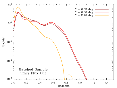
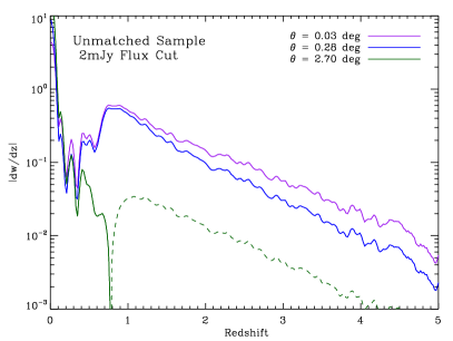
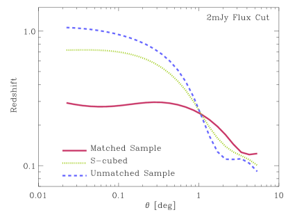
Figure 2: The top panels show contribution to the ACF ($d\omega_{\rm DM}/dz|_{\theta}$) at three different angles ($0.03^{\circ}$, $0.28^{\circ}$, $2.70^{\circ}$) as a function of redshift. Results are shown based on the redshift distributions of the matched and unmatched 2 mJy samples. The lower panel presents the average redshift, $\tilde{z}(\theta)$, which is probed at given angle for the three different samples indicated.

2.2 Redshift distribution comparison

We now compare our matched redshift distributions to that of the publicly available semi-empirical simulation of extragalactic radio continuum sources (S³) by Wilman et al. (2008) which is part of the SKA Simulated Skies (S³) project. The S³ covers a sky area of $20\times 20$ deg², out to a cosmological redshift of $z=20$. The simulated sources were drawn from observed (or extrapolated) luminosity functions and grafted onto an underlying dark matter density field with biases which reflect their measured large-scale clustering. For each source, which include FRII galaxies, FRI galaxies, radio-quiet quasars, starburst galaxies and star forming galaxies, the database gives the radio fluxes at observer frequencies of 151 MHz, 610 MHz, 1.4 GHz, 4.86 GHz and 18 GHz, down to flux density limits of 10 nJy. A prescription for clustering that captures the clustering pattern on large scales (larger than those where non-linear evolution of density fluctuations becomes important) was used. The simulations can be used to predict the redshift distribution of sources as a function of the flux cutoff of surveys.

Figure 1 shows the redshift distributions for our matched samples (solid lines) at the 7 mJy (red) and 2 mJy cuts (blue), compared to the S³ simulation (dotted line) for the same flux cuts. In general we find agreement between the observed matched and simulated redshift distributions up to $z\sim 0.5$. However, we do note that the prominent low redshift spike observed in the S³ data at $z\sim 0.04$ does not appear in our matched sample.

2.3 Clustering analysis

There are three different estimators that are used in the determination of two-point correlation function as originally developed by Davis and Huchra (1982), Hamilton (1993) and Landy and Szalay (1993). For this work, we apply the Landy and Szalay (1993) estimator, as it reduces errors caused by edges of catalogues and sub-samples during error calculation. This estimator can be written in the form:

$$\omega(\theta)=\frac{DD(\theta)-2DR(\theta)+RR(\theta)}{RR(\theta)}\ ,$$ (1)

where $DD(\theta)$ counts the number of pairs in the observed data as a function of angular scale. Similarly, $RR(\theta)$ counts the number pairs for the random catalogue and $DR(\theta)$ is the number of cross pairs between data and random catalogue. The integral constraint is negligable.

For our analysis we populated our random catalogue with 50 times the number of sources contained in the data for the matched and unmatched samples, and 100 times the data from the three redshift bins (cf., Table 2). The errors on $\omega$ were calculated using jack-knife re-sampling (Lupton, 1993). In this approach the data was split into $N=24$ bins in RA and the correlation function is recalculated repeatedly each time leaving out a different bin. A set of $N$ values $\{\omega_{i},i=1,...,N\}$ for the correlation function are obtained and the jack-knife error of the mean, $\sigma_{\omega_{mean}}$, is calculated by

$$\sigma_{\omega_{mean}}=\sqrt{(N-1)\sum^{N}_{i=1}(\omega_{i}-\omega)^{2}/N}\ .$$ (2)

Each of the 24 bins can be considered to be fairly independent due to the physical separation at the redshift probed.

In order to avoid problems associated with the over-cleaning of sidelobes, which effects the correlation function at $\theta\sim 0.2^{\circ}$, and any potential problems associated with collapsing multi-component sources, we only examine clustering at angles $\theta>0.4^{\circ}$. We are also concerned that measurements at angles larger than $\theta>1^{\circ}$ may be unreliable (see section 3).

2.4 Clustering predictions from CDM

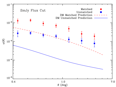
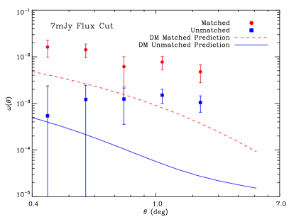
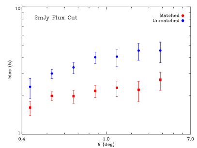
Figure 3: The two-point angular correlation function for the 2 mJy (left panel) and 7 mJy (right panel) matched and unmatched samples. In both panels the matched samples are indicated by blue points and the unmatched sample by the red points. The corresponding dark matter (DM) predictions are shown respectively by the dashed and solid lines. In the lower panel, we show the bias calculated for the 2 mJy flux cut of the matched (red) and the unmatched (blue) samples.

To determine the bias of the radio population we compare their ACF with the corresponding dark matter correlation function. If $q(z)$ is the normalised redshift distribution of a population of radio galaxies, the dark matter ACF can then be predicted from the non linear dark matter power spectrum ($P_{\rm DM}$) via Limber’s equation. For spatially flat cosmologies one derives the following expression.

$$\omega_{\rm DM}(\theta)=\int dr\ q^{2}(r)\int\frac{dk}{2\pi}k\ P_{\rm DM}(k,z)\ J_{0}[r(z)\theta k]$$ (3)

where $q(r)dr=q(z)dz$, $J_{0}(x)$ is the zeroth-order Bessel function of the first kind and $r(z)$ is the radial comoving distance. Here we adopt the fitting function for the non-linear CDM power spectrum by Peacock and Dodds (1996) using cosmological parameters given in Komatsu et al. (2009).

The linear bias, $b$, can be written

$$P_{lum}(k,z)=b^{2}(z,k)P_{\rm DM}(k,z)$$ (4)

where $P_{lum}$ is the power spectrum of luminous tracers of the dark matter. Here, we measure a bias parameter, $b_{\theta}$, in the angular clustering signal which samples $b(k,z)$ for radio sources in FIRST:

$$b_{\theta}=\sqrt{\frac{\omega_{\rm gal}}{\omega_{\rm DM}}}.$$ (5)

The derivative $d\omega_{\rm DM}/dz|_{\theta}$ at a given redshift $z$ reveals the contribution of that redshift slice to the overall ACF at the angle $\theta$. The upper panels of Figure 2 show $d\omega_{\rm DM}/dz|_{\theta}$ as a function of redshift for the matched and unmatched samples (left and right panel, respectively) at three different angles ($0.03^{\circ}$, $0.28^{\circ}$ and $2.70^{\circ}$). Based on that one can determine the average redshift, $\tilde{z}(\theta)$, which is probed at an angle $\theta$ for a given $q(z)$ by,

$$\tilde{z}(\theta)=\frac{\int z\ d\omega_{\rm DM}/dz|_{\theta}\ dz}{\int d\ \omega_{\rm DM}/dz|_{\theta}\ dz}\ .$$ (6)

The lower panel of Figure 2 shows $\tilde{z}(\theta)$ based on the redshift distributions of the SDSS matched and unmatched samples and the overall set of S³ sources. For small angels, $\sim 0.1^{\circ}$ the (un)matched sample probes redshifts of $z\sim 0.3(1.0)$. For angles above $1^{\circ}$ the average redshift probed is below $0.25$ irrespective of which sample is considered.

3 Results

3.1 The angular two-point correlation function (ACF)

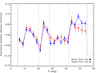
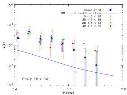
Figure 4: In the left panel we plot the fractional number density variation of the source density, with vertical lines indicating the declination strips used in the right panel . In the right panel we plot the ACF measured in four different declination strips roughly corresponding to different observing epochs: ($5^{\circ}-20^{\circ},20^{\circ}-28^{\circ},28^{\circ}-42^{\circ}$ and $42^{\circ}-55^{\circ}$)

Figure 3 shows the ACF for the 2mJy (left) and 7mJy (right) matched (red circles) and unmatched (blue squares) samples. In each panel the dark matter (DM) predictions are shown as dashed and solid lines, respectively. The bias (Equ. 5) is computed from the ratio between the data and predicted dark matter correlation functions and is shown as a function of angle in the lower panel for the 2mJy sample.

For the 2mJy cut, we see that the matched sample is more clustered (in angular projection) than the unmatched sample. This is expected since the matched sample occupies lower redshift ranges (cf., Fig. 1), thus a given angle corresponds to smaller physical scales where there is more clustering. The ACF for the full 1 mJy sample found by Cress et al. (1996) lies between our matched and unmatched curves. The amount of clustering measured in both the matched and unmatched samples at angles greater than $1^{\circ}$ is difficult to explain when one considers the results in Figure 2. On these scales, one would expect to probe $z\sim 0.1$ where the sample contains many fainter star-forming galaxies with a bias similar to normal galaxies i.e. $b_{\theta}\sim 1$. Instead, we see a bias $b_{\theta}>4$ for the unmatched and values $b_{\theta}>2$ for the matched sample.

To explore the possibility that large angle fluctuations are due to systematic variations in source density associated with different observing epochs, we plot fractional number density variation as a function of declination in the left panel of Figure 4 and note some fairly large changes in the fractional number density. To investigate the impact of this on the correlation function measurements, we divide the FIRST sources into declination strips roughly associated with different observing epochs and calculate the ACF in each strip. The results shown in the right panel of Figure 4 indicate that, beyond $1^{\circ}$, the results in the different declination strips start to differ. This suggests that systematics might have a significant effect on larger scales. However, we note that on smaller scales the measurements are consistent with each other, indicating that these scales are free of systematics related to this effect. We discuss other possible explanations for the excess large scale-power seen in the full sample in section 3.2 .

The right panel of Figure 3 shows the ACF for the 7mJy sample, which should be completely dominated by AGN (Best et al., 2003). The clustering of the matched sample is consistent with that of the 2mJy matched sample. In the unmatched sample, the bias is higher at large angles. The low measurements at smaller angles may indicate that the sidelobe over-cleaning problem is more pronounced for brighter sources.

To help interpret the matched ACF, we split the 2 mJy matched sample into three redshift slices, keeping the number of sources in each slice approximately constant. In the left panel of Figure 5, we plot the ACF for each of the redshift slices and in the right-hand panel we plot the bias calculated as a function of angle for each slice. One sees that the bias for the lowest redshift slice is fairly close to $b_{\theta}\sim 1$, as one would expect for a population dominated by fairly ordinary star-forming galaxies. Sources in the highest redshift bin are much more biased, as one would expect for a population dominated by AGN that trace large halo masses in the universe. The important point to note is that according to Figure 2 the average redshift probed for the matched sample at larger angles is about $z\sim 0.12$, but we see a large bias for the matched sample, left panel in Figure 3, at these angles and this can be attributed to the more highly biased population at $z>0.31$.

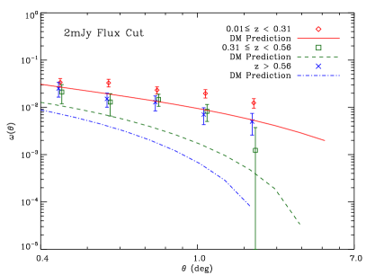
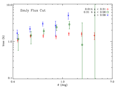
Figure 5: The left panel shows the ACF for the 2 mJy matched sample split into three redshift slices maintaining approximately the same number of objects in each slice. The three slices correspond to: $0.01\leq z<0.31$, (shown as red diamonds) $0.31\leq z<0.56$ (green squares) and $z>0.56$ (blue crosses). For each slice we have plotted the corresponding dark matter (DM) prediction. The right panel shows the evolution of bias for the three redshift slices.

Given that our main aim in this work is to constrain the bias toward high redshifts, we choose an angle of $0.66^{\circ}$ to determine the clustering behaviour of the high redshift radio sources. According to Figure 2 this choice allows us to probe bias at $z\sim 0.7$ . We find that the unmatched sources are more biased than the matched sample (at $3.3\sigma$), with a value of $b_{\theta}=3.0\pm 0.25$, compared to $2.0\pm 0.16$ for the matched sample at a mean redshift of $z\sim 0.7$.

Table 3: Bias results measured at an angle of 0.66^∘ for the matched, unmatched and the three redshift bins.

Samples	Bias ($b_{\theta}$)
Matched	2.0 $\pm 0.16$
Unmatched	3.0 $\pm 0.25$
$0.01\leq z<0.31$	1.4 $\pm 0.16$
$0.31\leq z<0.56$	1.5 $\pm 0.50$
$z>0.56$	2.2 $\pm 0.35$

3.2 Excess power at large angles

In this paper, our results are based on measurements at angles smaller than $1^{\circ}$ but it is interesting to consider explanations for the excess power at larger angles in the $unmatched$ sample.

1. Following the discussion for the matched sample, we could reason that, a highly biased population at high redshift could contribute significantly to the measurement at $\theta>1^{\circ}$, even though Figure 2 indicates that the average redshift probed on large angles is small. Bias of $b_{\theta}>4$, however, is not seen even for fairly massive clusters and additional contributors should be considered

2. Systematics other than those discussed in section 3.1 could also contribute. The beam shown in Condon et al. (1998) for the NVSS survey does not go to zero at large angles, suggesting that bright sources could produce artefacts at large angles due to imperfect cleaning in VLA data. However, similar ‘excess power’ is observed in the SUMSS radio survey which was carried out using a very different kind of telescope (Blake et al., 2004). Nevertheless, there is a possibility that radio surveys contain spurious sources which are correlated on large angles and this is a possible explanation for the excess power observed in clustering studies.

3. There is a low-redshift spike in the source counts, not included in the redshift distribution used for the dark matter predictions. This would push up the clustering amplitude on all angular scales, but particularly on the larger scales. However, the similar behaviour of the 2 and 7mJy indicate that the excess power is not due to faint, low-z star-forming galaxies. Also, the results of Magliocchetti et al. 2004 and Mauch and Sadler 2007 appear to rule out this explanation. The S³ redshift distribution which we use here is designed to fit these observations. A hypothetical low-redshift population which would have been missed in these studies would need to have $K>12.75$ and $B>19.45$, making such a low-z obscured population an unlikely explanation for much of the excess power in the unmatched sample.

4. Our matching technique is likely to result in some low-z multi-component radio sources being missed in our matched sample and one would expect these sources to be more biased than ordinary galaxies. This could boost the amplitude of clustering on large scales.

5. Finally, there is the possibility that non-gaussian initial conditions could generate more clustering on large scales than in the standard model as suggested by Xia et al. (2010).

Further work is clearly needed to understand the excess power in the clustering signal on large angles.

3.3 Consistency checks

We carried out a number of tests to check the robustness of our results. In the first test, we changed the matching radius to 1” to decrease the number of false identifications. This did not impact that ACF or the average redshift distribution of the unmatched sample, indicating that the bias measurement at $z\sim 0.7$ is not sensitive to the choice of matching radius. In the second test, we used the matched sample of Best et al. (2003) rather than our own matching. This sample was carefully constructed using both NVSS and FIRST and used visual identification rather than an automated “collapse and match” approach. Results were consistent with our matched sample, given that their sample probes a somewhat different redshift range to ours. In the third test, we considered the impact of our choice of sidelobe probability cut. We calculated the ACF for several different sidelobe probability samples and found that all samples behaved similarly at large angles. Finally, we investigated the sensitivity of our results to the photometric redshift estimates, by using different SDSS photometric redshift catalogues. We found that the results were robust to the choice of catalogue. .

4 Conclusions

We have introduced a method for measuring the bias at high redshift for a sample of radio continuum sources lacking redshift information. By matching radio sources from the FIRST survey data to their optical counterparts in the SDSS survey, we extracted a subsample of unmatched objects. We then used the S³ simulation to infer an average redshift distribution for all FIRST sources and estimate the redshift distribution of unmatched sources by subtracting the matched distribution from the distribution of all sources.

We have found that the surprisingly large clustering signal at large angular scales present in the full FIRST sample is also detected in the unmatched sample considered here, and to some extent, in the matched samples at high redshift. We note that this could be due to systematic fluctuations in sensitivity in different observing epochs but also discuss a number of other possible explanations. Using clustering measurements at smaller angles, we estimate the bias of the unmatched FIRST sources with flux densities over 2 mJy, at $z\sim 0.7$, to be $b_{\theta}=3.0\pm 0.25$.

The analysis of cross-correlations with other data will be helpful in interpreting these measurements better. These results can help constrain models of radio source evolution and are important for using radio surveys to constrain cosmological models.

5 Acknowledgements

The authors acknowledge the National Research Foundation and the SKA (South Africa) funding bodies, as well as the South African Astronomical Observatory (SAAO) and the Institute of Cosmology and Gravitation (ICG) where some of this work was carried out. The authors thank the African Institute for Mathematical Sciences (AIMS) for hosting the initial meeting where this project was concevied. RJ and MS would like to thank Prina Patel, Cris Sabiu and Luis Teodoro for valuable discussions.

References

- Abazajian et al. (2009) Abazajian, K. N., Adelman-McCarthy, J. K., Agüeros, M. A., Allam, S. S., Allende Prieto, C., An, D., Anderson, K. S. J., Anderson, S. F., Annis, J., Bahcall, N. A., and et al.: 2009, ApJ Suppl. 182, 543
- (2) Becker, R. H., White, R. L., and Helfand, D. J., in . J. B. D. R. Crabtree, R. J. Hanisch (ed.), Astronomical Data Analysis Software and Systems III
- Best et al. (2003) Best, P. N., Arts, J. N., Röttgering, H. J. A., Rengelink, R., Brookes, M. H., and Wall, J.: 2003, MNRAS 346, 627
- Blake et al. (2004) Blake, C., Mauch, T., and Sadler, E. M.: 2004, MNRAS 347, 787
- Blake and Wall (2002) Blake, C. and Wall, J.: 2002, MNRAS 329, L37
- Brookes et al. (2008) Brookes, M. H., Best, P. N., Peacock, J. A., Röttgering, H. J. A., and Dunlop, J. S.: 2008, MNRAS 385, 1297
- Brookes et al. (2006) Brookes, M. H., Best, P. N., Rengelink, R., and Röttgering, H. J. A.: 2006, MNRAS 366, 1265
- Carilli and Rawlings (2004) Carilli, C. L. and Rawlings, S.: 2004, New Astronomy Reviews 48, 979
- (9) Colless, M., The 2DF Galaxy Redshift Survey Team, Ellis, R., Bland-Hawthorn, J., Cannon, R., Cole, S., Collins, C., Couch, W., Dalton, G., Driver, S., and et al. ,, in R. M. . W. J. Couch (ed.), Looking Deep in the Southern Sky
- Condon et al. (1998) Condon, J. J., Cotton, W. D., Greisen, E. W., Yin, Q. F., Perley, R. A., Taylor, G. B., and Broderick, J. J.: 1998, A J 115, 1693
- Cress et al. (1996) Cress, C. M., Helfand, D. J., Becker, R. H., Gregg, M. D., and White, R. L.: 1996, Astrophys. J. 473, 7
- Cress and Kamionkowski (1998) Cress, C. M. and Kamionkowski, M.: 1998, MNRAS 297, 486
- Davis and Huchra (1982) Davis, M. and Huchra, J.: 1982, Astrophys. J. 254, 437
- Dunlop and Peacock (1990) Dunlop, J. S. and Peacock, J. A.: 1990, MNRAS 247, 19
- Hamilton (1993) Hamilton, A. J. S.: 1993, Astrophys. J. 417, 19
- Kamionkowski et al. (1998) Kamionkowski, M., Babul, A., Cress, C. M., and Refregier, A.: 1998, MNRAS 301, 1064
- Komatsu et al. (2009) Komatsu, E., Dunkley, J., Nolta, M. R., Bennett, C. L., Gold, B., Hinshaw, G., Jarosik, N., Larson, D., Limon, M., Page, L., Spergel, D. N., Halpern, M., Hill, R. S., Kogut, A., Meyer, S. S., Tucker, G. S., Weiland, J. L., Wollack, E., and Wright, E. L.: 2009, ApJ Suppl. 180, 330
- Landy and Szalay (1993) Landy, S. D. and Szalay, A. S.: 1993, Astrophys. J. 412, 64
- Lupton (1993) Lupton, R.: 1993, Statistics in theory and practice, Princeton Univ Pr
- Magliocchetti et al. (2004) Magliocchetti, M., Maddox, S. J., Hawkins, E., Peacock, J. A., Bland-Hawthorn, J., Bridges, T., Cannon, R., Cole, S., Colless, M., Collins, C., and et al. ,: 2004, MNRAS 350, 1485
- Mauch and Sadler (2007) Mauch, T. and Sadler, E. M.: 2007, MNRAS 375, 931
- Mo and White (1996) Mo, H. J. and White, S. D. M.: 1996, MNRAS 282, 347
- Nolta et al. (2004) Nolta, M. R., Wright, E. L., Page, L., Bennett, C. L., Halpern, M., Hinshaw, G., Jarosik, N., Kogut, A., Limon, M., Meyer, S. S., and et al. ,: 2004, Astrophys. J. 608, 10
- Overzier et al. (2003) Overzier, R. A., Röttgering, H. J. A., Rengelink, R. B., and Wilman, R. J.: 2003, A&A 405, 53
- Oyaizu et al. (2008) Oyaizu, H., Lima, M., Cunha, C. E., Lin, H., and Frieman, J.: 2008, Astrophys. J. 689, 709
- Peacock and Dodds (1996) Peacock, J. A. and Dodds, S. J.: 1996, MNRAS 280, L19
- Raccanelli (2011) Raccanelli, A.: 2011, Journal of Physics Conference Series 280(1), 012009
- Raccanelli et al. (2008) Raccanelli, A., Bonaldi, A., Negrello, M., Matarrese, S., Tormen, G., and de Zotti, G.: 2008, MNRAS 386, 2161
- Rengelink et al. (1997) Rengelink, R. B., Tang, Y., de Bruyn, A. G., Miley, G. K., Bremer, M. N., Roettgering, H. J. A., and Bremer, M. A. R.: 1997, A&AS 124, 259
- Waddington et al. (2001) Waddington, I., Dunlop, J. S., Peacock, J. A., and Windhorst, R. A.: 2001, MNRAS 328, 882
- (31) Wakamatsu, K., Colless, M., Jarrett, T., Parker, Q., Saunders, W., and Watson, F., in . T. H. S. Ikeuchi, J. Hearnshaw (ed.), The Proceedings of the IAU 8th Asian-Pacific Regional Meeting, Volume I
- Wilman et al. (2010) Wilman, R. J., Jarvis, M. J., Mauch, T., Rawlings, S., and Hickey, S.: 2010, MNRAS 405, 447
- Wilman et al. (2008) Wilman, R. J., Miller, L., Jarvis, M. J., Mauch, T., Levrier, F., Abdalla, F. B., Rawlings, S., Klöckner, H., Obreschkow, D., Olteanu, D., and Young, S.: 2008, MNRAS 388, 1335
- Xia et al. (2010) Xia, J.-Q., Bonaldi, A., Baccigalupi, C., De Zotti, G., Matarrese, S., Verde, L., and Viel, M.: 2010, J. Cosmology Astropart. Phys. 8, 13