DESY 12-197

TIT/HEP-623

UTHEP-652

Null-polygonal minimal surfaces in AdS₄ from perturbed $W$ minimal models
Yasuyuki Hatsuda, Katsushi Ito and Yuji Satoh
^∗DESY Theory Group, DESY Hamburg
D-22603 Hamburg, Germany ^∗,†Department of Physics, Tokyo Institute of Technology
Tokyo, 152-8551, Japan ^‡Institute of Physics, University of Tsukuba
Ibaraki, 305-8571, Japan

We study the null-polygonal minimal surfaces in AdS₄, which correspond to the gluon scattering amplitudes/Wilson loops in ${\cal N}=4$ super Yang-Mills theory at strong coupling. The area of the minimal surfaces with $n$ cusps is characterized by the thermodynamic Bethe ansatz (TBA) integral equations or the Y-system of the homogeneous sine-Gordon model, which is regarded as the $\mathrm{SU}(n-4)_{4}/\mathrm{U}(1)^{n-5}$ generalized parafermion theory perturbed by the weight-zero adjoint operators. Based on the relation to the TBA systems of the perturbed $W$ minimal models, we solve the TBA equations by using the conformal perturbation theory, and obtain the analytic expansion of the remainder function around the UV/regular-polygonal limit for $n=6$ and $7$. We compare the rescaled remainder function for $n=6$ with the two-loop one, to observe that they are close to each other similarly to the AdS₃ case.

November 2012

1 Introduction

The AdS/CFT correspondence shows that minimal surfaces in AdS space-time are dual to the Wilson loops along their boundary [1, 2], where the area corresponds to the expectation value of the Wilson loops at strong coupling. When the boundary is null-polygonal/light-like, the minimal surfaces also give the gluon scattering amplitudes of ${\cal N}=4$ super Yang-Mills theory [3], implying the duality between the amplitudes and the Wilson loops [3, 4, 5] and hence the dual conformal symmetry [3, 6, 7] . This dual conformal symmetry completely fixes the $n$-point amplitudes/Wilson loops with $n$ cusps up to $n=5$. For $n\geq 6$, however, it allows deviation from the Bern-Dixon-Smirnov (BDS) formula [8] by the remainder function [9, 10, 11], which is a function of the cross-ratios of the cusp coordinates on the boundary.

At strong coupling, the corresponding area of the minimal surfaces is evaluated with the help of integrability [12]. More concretely, one first solves a set of integral equations of the thermodynamic Bethe ansatz (TBA) form, or an associated Y-/T-system [13, 14, 15]. The cross-ratios are then expressed by its solution, i.e., the Y- or T-functions, and consequently the main part of the remainder function is given by these Y-/T-functions as well as the free energy associated with the TBA system.

In a previous paper [15], Sakai and the present authors pointed out that the TBA equations for the minimal surfaces with $2\tilde{n}$ cusps in AdS₃ coincide with those of the $\mathrm{SU}(\tilde{n}-2)_{2}/\mathrm{U}(1)^{\tilde{n}-3}$ homogeneous sine-Gordon (HSG) model [16] with purely imaginary resonance parameters. Similarly, it was inferred there that the TBA equations for the minimal surfaces with $n$ cusps in AdS₄ are those of the HSG model associated with $\mathrm{SU}(n-4)_{4}/\mathrm{U}(1)^{n-5}$.

These observations allow us to solve the TBA systems around the UV/high-temperature limit, where the two-dimensional integrable (HSG) model reduces to a conformal field theory (CFT). The deviation from the UV limit then corresponds to an integrable relevant/mass perturbation of the CFT. The corrections to observables are also regarded as finite size effects of the two-dimensional system, which can be computed by using the conformal perturbation theory (CPT). By the standard procedure [17], one can indeed derive an analytic expansion of the free energy around the UV limit. The Y-/T-functions are also expanded by the CPT with boundaries [18, 19], based on the relation to the $g$-function (boundary entropy) [20]. Since the Wilson loops become regular polygonal in the UV limit, those expansions give an analytic expansion of the remainder function around this regular-polygonal limit. For the analysis in the opposite IR/large-mass regime, see [12, 13, 21, 22, 23, 24, 25].

We have carried out the above program for the minimal surfaces embedded in AdS₃ [26, 27]. In this case, the relevant CFT is the $\mathrm{SU}(\tilde{n}-2)_{2}/\mathrm{U}(1)^{\tilde{n}-3}$ generalized parafermion theory [28] and, by turning off some mass parameters so as to leave only one mass scale (single-mass case), the TBA system is reduced to simpler ones for the perturbed $\mathrm{SU}(2)$ diagonal coset and minimal models. This is a key step which enables us to find precise values of the expansion coefficients in terms of the mass parameters in the TBA system, through the relation to the coupling of the relevant perturbation (mass-coupling relation) and the correlation functions. We then derived the expansion of the 8- and 10-point remainder functions in [26], and that of the general $2\tilde{n}$-point remainder function in [27]. We observed that the appropriately rescaled remainder functions are close to those evaluated at two loops [29, 30, 31].

The purpose of the present work is to study the analytic expression of the regularized area of the null-polygonal minimal surfaces in AdS₄ by extending the above results in the AdS₃ case. In particular, we derive the analytic expansion of the remainder function around the UV limit by using the underlying integrable models and the CPT. In this case, the corresponding TBA or Y-system is obtained by a projection from that for the minimal surfaces in AdS₅ [14]. The relevant CFT in the UV limit for the $n$-cusp surfaces is now the $\mathrm{SU}(n-4)_{4}/\mathrm{U}(1)^{n-5}$ generalized parafermion theory. The TBA systems with only one mass parameter are given by those for the perturbed unitary $\mathrm{SU}(4)$ diagonal coset models and $W$ minimal models. We also argue that a similar correspondence to the perturbed non-unitary diagonal coset and $W$ minimal models holds for the systems with a pair of equal mass parameters. These generalize the reduction in the AdS₃ case, and are used to find the precise expansion coefficients. Explicitly, we work out the leading-order expansion for $n=6$ and $7$. In these cases, the input from the perturbed $W$ minimal models completely determines the leading-order expansion. For $n=6$, we also compare the rescaled remainder function with the two-loop one which is read off from [32, 33, 34, 35], to observe that they are close to each other.

This paper is organized as follows: In section 2, we review the remainder function corresponding to the minimal surfaces in AdS₄, and the associated TBA system. We explicitly check that the TBA equations for the $n$-cusp minimal surfaces are obtained from the $\mathrm{SU}(n-4)_{4}/\mathrm{U}(1)^{n-5}$ homogeneous sine-Gordon model. In section 3, we discuss the TBA systems in the single-mass cases in relation to the perturbed $\mathrm{SU}(4)$ diagonal coset and $W$ minimal models. In section 4, we discuss the expansion of the free energy, and derive the leading-order expansion for $n=6$ and $7$. In section 5, we extend the formalism of the expansion of the T-/Y-functions to the AdS₄ case, and derive the leading-order expansion for $n=6$ and $7$. Combining those results, we derive the analytic expansion of the remainder function for $n=6$ and $7$ in section 6. We also compare the rescaled remainder function for $n=6$ with the two-loop one. In the appendix, we summarize a computation of a three-point function in a non-unitary $W$ minimal model.

2 TBA equations for minimal surfaces in AdS₄

In this section, we review the computation of the regularized area of the minimal surfaces in the AdS space with a null polygonal boundary using integrability. As studied in [13, 14, 15], such an area is governed by a set of non-linear integral equations of the TBA form or the associated T-/Y-systems. Those equations coincide with the TBA equations of the homogeneous sine-Gordon model.

2.1 Functional relations and TBA equations

The basic idea to compute the area of the minimal surfaces is as follows. We start with the non-linear sigma model that describes the classical strings in AdS₅. After the Pohlmeyer reduction, the equations of motion for classical strings are mapped to a linear system of differential equations. Due to the integrability of the linear system, one can introduce a spectral parameter $\theta$. Using the bispinor representation, this system is brought to the $\mathrm{SU}(4)$ Hitchin system with a ${\mathbb{Z}}_{4}$-symmetry. Solutions of this linear problem show the Stokes phenomena [12]. The smallest solution is uniquely determined in each Stokes sector. Their Wronskians evaluated at special values of the spectral parameter form the cross-ratios of the cusp coordinates. From the Plücker relations, these Wronskians satisfy certain functional relations called the T-system.

For AdS₅, it reads as the following relations among the T-functions $T_{a,s}(\theta)$,

$$T_{a,s}^{+}T_{4-a,s}^{-}=T_{4-a,s+1}T_{a,s-1}+T_{a+1,s}T_{a-1,s}\,,$$ (2.1)

where $a=1,2,3$; $s=1,2,\cdots,n-5$ for the $n$-cusp minimal surfaces and $f^{\pm}(\theta):=f(\theta\pm{i\pi\over 4})$. The boundary conditions for the T-functions are

$$T_{a,0}=1\ (a=1,2,3),\quad T_{0,s}=T_{4,s}=1\ (s\in{\mathbb{Z}}).$$ (2.2)

At the boundary $s=n-4$, we have also to impose the boundary condition related to the formal monodromy [14]. For $n\not\in 4\mathbb{Z}$, the condition is simply given by

$$T_{1,n-4}=\mu^{-(1+(-1)^{n})/2},\quad T_{2,n-4}=1,\quad T_{3,n-4}=\mu^{(1+(-1)^{n})/2},$$ (2.3)

where $\mu$ is a constant. In this work, we focus on this $n\notin 4{\mathbb{Z}}$ case, where we do not need to consider extra monodromy factors. From the T-functions, the Y-functions are defined by

$$Y_{a,s}=\frac{T_{a,s+1}T_{4-a,s-1}}{T_{a+1,s}T_{a-1,s}}.$$ (2.4)

They satisfy a set of functional relations called the Y-system:

$$\frac{Y_{a,s}^{-}Y_{4-a,s}^{+}}{Y_{a+1,s}Y_{a-1,s}}=\frac{(1+Y_{a,s+1})(1+Y_{4-a,s-1})}{(1+Y_{a+1,s})(1+Y_{a-1,s})}.$$ (2.5)

The boundary conditions for the Y-functions are $Y_{a,0}=Y_{a,n-4}=0$ ($a=1,2,3$) and $Y_{0,s}=Y_{4,s}=\infty$ ($s=1,\cdots,n-5$). The Y-system has many solutions in general. To determine a solution of the Y-system, we need to know the analytic structure of the Y-functions including their asymptotics for large $|\theta|$, which has been studied in [14]. The asymptotics is specified by auxiliary complex (mass) parameters $m_{s}$ and constants $C_{s},D_{s}$. For real $m_{s}$, it is given by

$$\log Y_{1,s}(\theta) \to-m_{s}\cosh\theta-C_{s}\pm D_{s}\,,$$

$$\log Y_{2,s}(\theta) \to-\sqrt{2}m_{s}\cosh\theta\,,$$ (2.6)

$$\log Y_{3,s}(\theta) \to-m_{s}\cosh\theta+C_{s}\mp D_{s}\,,$$

as $\theta\to\pm\infty$. One can show that the Y-system can be rewritten into a set of integral equations of the TBA form. Those equations for the minimal surfaces in the AdS₅ space are given by

$$\log Y_{1,s}(\theta) =-m_{s}\cosh\theta-C_{s}-K_{1}*\alpha_{s}-\frac{1}{2}K_{2}*\beta_{s}-\frac{1}{2}K_{3}*\gamma_{s},$$

$$\log Y_{2,s}(\theta) =-\sqrt{2}m_{s}\cosh\theta-K_{2}*\alpha_{s}-K_{1}*\beta_{s},$$ (2.7)

$$\log Y_{3,s}(\theta) =-m_{s}\cosh\theta+C_{s}-K_{1}*\alpha_{s}-\frac{1}{2}K_{2}*\beta_{s}+\frac{1}{2}K_{3}*\gamma_{s},$$

where $\ast$ stands for the convolution, $f\ast g:=\int_{-\infty}^{\infty}d\theta\,f(\theta-\theta^{\prime})g(\theta^{\prime})$. The functions $\alpha_{s}$, $\beta_{s}$ and $\gamma_{s}$ are defined by

$$\alpha_{s} =\log\frac{(1+Y_{1,s})(1+Y_{3,s})}{(1+Y_{2,s-1})(1+Y_{2,s+1})},\qquad\gamma_{s}=\log\frac{(1+Y_{1,s-1})(1+Y_{3,s+1})}{(1+Y_{1,s+1})(1+Y_{3,s-1})},$$

$$\beta_{s} =\log\frac{(1+Y_{2,s})^{2}}{(1+Y_{1,s-1})(1+Y_{1,s+1})(1+Y_{3,s-1})(1+Y_{3,s+1})},$$ (2.8)

and the kernels are by

$$K_{1}(\theta)=\frac{1}{2\pi\cosh\theta},\qquad K_{2}(\theta)=\frac{\sqrt{2}\cosh\theta}{\pi\cosh 2\theta},\qquad K_{3}(\theta)=\frac{i}{\pi}\tanh 2\theta.$$ (2.9)

The constants $D_{s}$ are obtained from $\gamma_{s}$ by $D_{s}=\frac{i}{\pi}\int d\theta\,\gamma_{s}(\theta)$, whereas the constant $\mu$ in (2.3) is related to $C_{s}$.

In this paper, we particularly focus on the minimal surfaces in the AdS₄ subspace, which correspond to the amplitudes with the four-momenta of the external particles lying in a three-dimensional subspace. In this case, the above integral equations are simplified to the TBA equations of a known integrable system. To reduce the problem into AdS₄, we need a projection of the original system for the AdS₅ space. This projection relates the smallest solutions of the linear problem to those for the inverse problem via a gauge transformation. This relation results in the following conditions in the TBA system,

$$T_{1,s}(\theta)=T_{3,s}(\theta),\qquad Y_{1,s}(\theta)=Y_{3,s}(\theta),$$ (2.10)

where the latter relation leads to $\mu^{2}=1$. In this paper, we particularly consider the case with $\mu=1$ and $C_{s}=0$, so that one can analyze the area for small $m_{s}$ by the underlying integrable models and conformal field theories. Then, we obtain the simplified integral equations,

$$\log Y_{1,s}(\theta) =-m_{s}\cosh\theta-K_{1}*\alpha_{s}-\frac{1}{2}K_{2}*\beta_{s},$$

$$\log Y_{2,s}(\theta) =-\sqrt{2}m_{s}\cosh\theta-K_{2}*\alpha_{s}-K_{1}*\beta_{s},$$ (2.11)

where $\alpha_{s}$ and $\beta_{s}$ reduce to

$$\alpha_{s}=\log\frac{(1+Y_{1,s})^{2}}{(1+Y_{2,s-1})(1+Y_{2,s+1})},\qquad\beta_{s}=2\log\frac{(1+Y_{2,s})}{(1+Y_{1,s-1})(1+Y_{1,s+1})}.$$ (2.12)

So far, we have focused on the real mass $(m_{s})$ case. One can generalize these results to the complex-mass case as in [14]. If the masses in the TBA equations are complex, $m_{s}=|m_{s}|e^{i\varphi_{s}}$, the driving terms of the TBA equations are modified as

$$-m_{a,s}\cosh\theta\to-\frac{1}{2}(\bar{m}_{a,s}e^{\theta}+m_{a,s}e^{-\theta})=-\frac{|m_{a,s}|}{2}(e^{\theta-i\varphi_{s}}+e^{-(\theta-i\varphi_{s})}),$$ (2.13)

where $m_{1,s}=m_{2,s}/\sqrt{2}=m_{s}$. Thus, defining $\tilde{Y}_{a,s}(\theta)=Y_{a,s}(\theta+i\varphi_{s})$, the TBA equations become

$$\log\tilde{Y}_{1,s} =-|m_{s}|\cosh\theta-2K_{1}*\log(1+\tilde{Y}_{1,s})$$

$$\hskip 14.22636pt+K_{1}^{s,s-1}*\log(1+\tilde{Y}_{2,s-1})+K_{1}^{s,s+1}*\log(1+\tilde{Y}_{2,s+1})$$

$$\hskip 14.22636pt-K_{2}*\log(1+\tilde{Y}_{2,s})+K_{2}^{s,s-1}*\log(1+\tilde{Y}_{1,s-1})+K_{2}^{s,s+1}*\log(1+\tilde{Y}_{1,s+1}),$$

$$\log\tilde{Y}_{2,s} =-\sqrt{2}|m_{s}|\cosh\theta-2K_{2}*\log(1+\tilde{Y}_{1,s})$$ (2.14)

$$\hskip 14.22636pt+K_{2}^{s,s-1}*\log(1+\tilde{Y}_{2,s-1})+K_{2}^{s,s+1}*\log(1+\tilde{Y}_{2,s+1})$$

$$\hskip 14.22636pt-2K_{1}*\log(1+\tilde{Y}_{2,s})+2K_{1}^{s,s-1}*\log(1+\tilde{Y}_{1,s-1})+2K_{1}^{s,s+1}*\log(1+\tilde{Y}_{1,s+1}),$$

where

$$K_{j}^{s,s^{\prime}}(\theta)=K_{j}(\theta+i\varphi_{s}-i\varphi_{s^{\prime}})\qquad(j=1,2).$$ (2.15)

Note that this integral equations are valid only when $|\varphi_{s}-\varphi_{s^{\prime}}|<\pi/4$ for all $s,s^{\prime}$. If at least one of $|\varphi_{s}-\varphi_{s^{\prime}}|$ is greater than $\pi/4$, we need to modify the TBA equations due to the poles in the kernels. The complex masses $m_{s}$ provide $2(n-5)$ independent real parameters for the TBA system, which match the number of the independent cross-ratios formed by the cusp coordinates of the AdS₄ minimal surfaces.

2.2 TBA equations for $\mathrm{SU}(N)_{4}/\mathrm{U}(1)^{N-1}$ HSG model

In [15], the integral equations for the $2\tilde{n}$-cusp null-polygonal minimal surfaces in AdS₃ were identified with the TBA equations of the $\mathrm{SU}(\tilde{n}-2)_{2}/\mathrm{U}(1)^{\tilde{n}-3}$ HSG model with purely imaginary resonance parameters $\sigma_{s}=i\varphi_{s}$, where the masses of the particles are regarded as complex parameters. The corresponding relation was also inferred in the same paper between the present $n$-cusp minimal surfaces in AdS₄ and the $\mathrm{SU}(n-4)_{4}/\mathrm{U}(1)^{n-5}$ HSG model. The relation is indeed confirmed by comparing the integral equations in the previous subsection with the TBA equations of this HSG model, which are read off from the general expression in [36]. Let us see this explicitly below.

For this purpose, we first recall that the HSG model associated with the $\mathrm{SU}(N)$ coset is defined as an integrable perturbation of the $\mathrm{SU}(N)_{k}/\mathrm{U}(1)^{N-1}$ gauged WZNW/generalized parafermion model by the weight-zero primary fields in the adjoint representation of $\mathfrak{su}(N)$. Here, we denote the $\mathrm{SU}(N)$ affine Lie algebra at level $k$ by $\mathrm{SU}(N)_{k}$. This $\mathrm{SU}(N)_{k}/\mathrm{U}(1)^{N-1}$ coset CFT has the central charge,

$$c({\mathrm{SU}(N)_{k}\over\mathrm{U}(1)^{N-1}})={(k-1)N(N-1)\over k+N}\,,$$ (2.16)

and its primary field $\Phi^{\boldsymbol{\Lambda}}_{\boldsymbol{\lambda}}(z)$ with weight $\boldsymbol{\lambda}$ in the highest-weight representation labeled by $\boldsymbol{\Lambda}$ has the conformal dimension,

$$\Delta^{\boldsymbol{\Lambda}}_{\boldsymbol{\lambda}}={\boldsymbol{\Lambda}(\boldsymbol{\Lambda}+2\boldsymbol{\rho}_{\mathfrak{su}(N)})\over 2(k+N)}-{\boldsymbol{\lambda}^{2}\over 2k}.$$ (2.17)

$\boldsymbol{\rho}_{\mathfrak{su}(N)}$ is half the sum of the positive roots (the Weyl vector) of the Lie algebra $\mathfrak{su}(N)$. The action of the HSG model then takes the form,

$$S_{\rm HSG}=S_{\rm gWZNW}+\lambda\int d^{2}x\,\Phi\,,$$ (2.18)

where $\Phi$ is a combination of the weight-zero adjoint operators $\Phi^{\boldsymbol{\omega}_{1}+\boldsymbol{\omega}_{N-1}}_{\bf 0}$, which is parametrized by the $N-1$ real mass parameters $M_{s}$ ($s=1,\cdots,N-1$) and the real resonance parameters $\sigma_{s}$. This perturbing operator $\Phi$ has the dimension,

$$\Delta=\bar{\Delta}:=\Delta^{\boldsymbol{\omega}_{1}+\boldsymbol{\omega}_{N-1}}_{\bf 0}={N\over N+k}\,.$$ (2.19)

On dimensional grounds, the coupling of the integrable relevant/mass perturbation is expressed by the dimensionless coupling $\kappa$ and the mass scale $M$ as

$$\lambda=-\kappa M^{2-\Delta-\bar{\Delta}}\,.$$ (2.20)

We note that the above action describes a multi-parameter integrable perturbation, which is a notable feature of the HSG model.

The particles in this model are labeled by two quantum numbers $(a,s)$ and have masses

$$M_{a,s}=M_{s}\sin\bigl{(}\frac{\pi a}{k}\bigr{)}/\sin\bigl{(}\frac{\pi}{k}\bigr{)}\,,$$ (2.21)

where $a=1,...,k-1$. The S-matrix of the diagonal scattering between the particles $(a,r)$ and $(b,s)$ is then given by [37]

$$S_{ab}^{rs}(\theta;\sigma_{rs})=\Bigl{[}S^{\rm min}_{ab}(\theta)\Bigr{]}^{\delta_{r,s}}\Bigl{[}(\eta_{r,s})^{-ab}S^{F}_{ab}(\theta+\sigma_{rs})\Bigr{]}^{-I_{rs}}\,,$$ (2.22)

where $\sigma_{rs}:=\sigma_{r}-\sigma_{s}$, and

$$S_{ab}^{\rm min}(\theta)=\prod_{j=0}^{{\rm min}(a,b)-1}(a+b-2j)_{\theta}(a+b-2-2j)_{\theta}$$ (2.23)

with

$$(x)_{\theta}:=\frac{\sinh\frac{1}{2}\bigl{(}\theta+\frac{i\pi}{k}x\bigr{)}}{\sinh\frac{1}{2}\bigl{(}\theta-\frac{i\pi}{k}x\bigr{)}}$$ (2.24)

is the S-matrix of the $A_{k-1}$ minimal affine Toda field theory (ATFT) [38, 39]. In the second factor, $I_{rs}=\delta_{r,s+1}+\delta_{r,s-1}$ is the incidence matrix of the Lie algebra $\mathfrak{su}(N)$, $\eta_{r,s}(=\eta_{s,r}^{-1})$ are arbitrary $k^{\rm th}$ roots of $-1$, and $S_{ab}^{F}$ is given by

$$S_{ab}^{F}(\theta)=\prod_{j=0}^{{\rm min}(a,b)-1}(a+b-1-2j)_{\theta}\,.$$ (2.25)

The parity-invariance of $S_{ab}^{rs}$ is broken due to $\eta_{r,s}$ and $\sigma_{rs}$.

Next, we recall that, for a diagonal scattering theory with the S-matrix $S_{AB}$, the TBA equations in the fermionic case take the form (see for example [40]),

$$\log Y_{A}(\theta)=-m_{A}\cosh\theta+\sum_{B}K_{AB}\ast\log(1+Y_{B})\,,$$ (2.26)

where $K_{AB}(\theta)$ are the kernels defined by

$$K_{AB}(\theta)=\frac{1}{2\pi i}\frac{\partial}{\partial\theta}\log S_{AB}(\theta)\,.$$ (2.27)

On the right-hand side, $m_{A}=M_{A}L$ is the dimensionless combination of the mass parameter $M_{A}$ and the length scale/inverse temperature $L$. We have also assumed above that the kernels are symmetric: $K_{AB}(\theta)=K_{BA}(\theta)$. Once the resonance parameters are set to be vanishing, $\sigma_{rs}=0$, the kernels for the HSG model are indeed symmetric and one can apply this formula.

From the resultant TBA equations, one can show that $Y_{1,s}=Y_{3,s}$ for $k=4$. After imposing this condition, we find that the TBA equations of the $\mathrm{SU}(N)_{4}/\mathrm{U}(1)^{N-1}$ HSG model with vanishing $\sigma_{s}$ are just the same as the integral equations (2.11) for the $(N+4)$-cusp minimal surfaces in AdS₄ with real mass parameters. Here, the correspondences of the parameters are $m_{1,s}=m_{3,s}=m_{2,s}/\sqrt{2}=m_{s}$ for the masses $m_{A}=m_{a,s}$, and

$$K_{12}^{rs}=K_{23}^{rs}=K_{1}\,,\quad K_{22}^{rs}=K_{11}^{rs}+K_{13}^{rs}=K_{33}^{rs}+K_{13}^{rs}=K_{2}\,,$$ (2.28)

for the kernels $K_{AB}=K_{ab}^{rs}$. When the mass parameters are complex, $m_{s}=|m_{s}|e^{i\varphi_{s}}$, the phases correspond to the purely imaginary resonance parameters $\sigma_{s}=i\varphi_{s}$. One finds that the TBA equations in this case are given by (2.14).

2.3 Remainder function

In the previous two subsections, we have seen that the null-polygonal minimal surfaces with $n$ cusps in AdS₄ are characterized by the TBA equations for the SU($n-4$)₄/U(1)^n-5 HSG model. We would like to know the area of such minimal surfaces. Here we see that the area can be expressed in terms of the T-/Y-functions, the free energy and the mass parameters associated with the TBA system.

The area shows divergence, since the surfaces extend to the boundary of AdS at infinity and have the cusp points there. Introducing the radial-cutoff, the regularized area is given by the Stokes data of the linear problem. For the $n$-cusp minimal surfaces, it takes the form,

$$A_{n}=A_{\rm div}+A_{\rm BDS-like}+A_{\rm periods}+A_{\rm free},$$ (2.29)

where $A_{\rm div}$ is the divergent part, $A_{\rm periods}$ is the period part which depends on the mass parameters governing the asymptotics of the Y-functions. $A_{\rm BDS-like}$ is given by distances among the cusp points, which is similar to the BDS expression but different. $A_{\rm free}$ is the free energy associated with the TBA system.

The remainder function is now defined by the difference between the regularized area and the BDS formula,

$$A_{n}=A_{\rm div}+A_{\rm BDS}+R_{n}\,.$$ (2.30)

The explicit form of the remainder function at strong coupling is then given by

$$R_{n}=\Delta A_{\rm BDS}+A_{\rm periods}+A_{\rm free}\,.$$ (2.31)

The first term $\Delta A_{\rm BDS}:=A_{\rm BDS\mbox{-}like}-A_{\rm BDS}$ is expressed in terms of the cross-ratios, and its general expression for $n\notin 4{\mathbb{Z}}$ is found in [13]. Here, we list the expressions for $n=6$ and $7$, which are used in the following sections:

$$\Delta A_{\rm BDS}^{(n=6)} = -\frac{1}{4}\sum_{i=1}^{3}\Bigl{[}\frac{1}{2}\log^{2}u_{i,i+3}+\operatorname{Li_{2}}(1-u_{i,i+3})\Bigr{]}=\frac{1}{4}\sum_{i=1}^{3}\operatorname{Li_{2}}\Bigl{(}1-\frac{1}{u_{i,i+3}}\Bigr{)}\,,$$ (2.32)

for $n=6$ and

$$\Delta A_{\rm BDS}^{(n=7)} = -\frac{1}{4}\sum_{i=1}^{7}\Bigl{[}\log^{2}u_{i,i+3}-\frac{1}{2}\log u_{i,i+3}\log\frac{u_{i+2,i+5}u_{i+1,i+5}}{u_{i+3,i+6}u_{i,i+4}}+\operatorname{Li_{2}}(1-u_{i,i+3})\Bigr{]}\,,\qquad$$ (2.33)

for $n=7$ (see also [23]). The cross-ratios $u_{i,j}$ above are defined by

$$u_{i,j}:=\frac{x^{2}_{i,j+1}x^{2}_{i+1,j}}{x^{2}_{i,j}x^{2}_{i+1,j+1}}\,,$$ (2.34)

and the cusps are labeled modulo $n$. These cross-ratios are concisely expressed by the Y-/T-functions through

$$U_{s}^{[r]}:=1+\frac{1}{Y_{2,s}^{[r]}}=\frac{T_{2,s}^{[r+1]}T_{2,s}^{[r-1]}}{T_{2,s+1}^{[r]}T_{2,s-1}^{[r]}}$$ (2.35)

with $f^{[r]}:=f(\theta=i\pi r/4)$ as follows [14],

$$U_{2k-2}^{[0]}=\frac{1}{u_{k-1,-k-1}}\,,\qquad U_{2k-1}^{[-1]}=\frac{1}{u_{k-1,-k-2}}\,.$$ (2.36)

Other cross-ratios are generated by the ${\mathbb{Z}}_{n}$-symmetry, $x_{i}^{\mu}\to x_{i+1}^{\mu}$, which corresponds to the shift of the argument

$$Y_{a,s}^{[r]}\to Y_{a,s}^{[r+2]}\,,\qquad T_{a,s}^{[r]}\to T_{a,s}^{[r+2]}\,.$$ (2.37)

In addition, other parts $A_{\rm periods}$ and $A_{\rm free}$ are given by

$$A_{\rm periods} =\sum_{s,s^{\prime}=1}^{n-5}{\cal K}_{ss^{\prime}}m_{s}\bar{m}_{s^{\prime}},$$

$$A_{\rm free} =\sum_{s=1}^{n-5}\int_{-\infty}^{\infty}\frac{d\theta}{2\pi}|m_{s}|\cosh\theta\log\Bigl{[}(1+\tilde{Y}_{1,s}(\theta))^{2}(1+\tilde{Y}_{2,s}(\theta))^{\sqrt{2}}\Bigr{]}.$$ (2.38)

The explicit forms of ${\cal K}_{ss^{\prime}}$ are found in [14] for $n\not\in 4\mathbb{Z}$, and are conjectured in [21] for $n\in 4\mathbb{Z}$. Here we list the results for $n=6,7$ only:

$${\cal K}^{(n=6)}=\frac{1}{4},\qquad{\cal K}^{(n=7)}=\frac{1}{2\sqrt{2}}\begin{pmatrix}\sqrt{2}&1\\ 1&\sqrt{2}\end{pmatrix}.$$ (2.39)

Although $\Delta A_{\rm BDS}$ is given by the cross-ratios directly, $A_{\rm periods}$ and $A_{\rm free}$ are related to the cross-ratios indirectly through the Y-/T-functions and the mass parameters. Indeed, the Y-functions are uniquely determined by solving the TBA equations for given masses and, once $Y_{a,s}$ are obtained in terms of $m_{s}$, the mass parameters and hence the Y-/T-functions are related to the cross-rations through (2.35). As a result, the remainder function at strong coupling is expressed as a function of the cross-ratios.

2.4 UV expansion

In the following sections, we discuss an analytic expansion of the remainder function around the high-temperature/UV limit, where the mass parameters $m_{s}$ become vanishing and the corresponding Wilson loops become regular-polygonal. This is achieved by several steps: First, we note that around this limit the deformation term in (2.18) is treated as a small-mass perturbation for the coset/generalized parafermion CFT [28]. Then, the free energy of the TBA system, which is given by the ground-state energy in the mirror channel, is obtained analytically by the conformal perturbation theory [17]. It is expanded in terms of the correlation functions of the deformation operator $\Phi$. Next, we use the relation between the Y-/T-function and the $g$-function [20]. The $g$-function is regarded as a boundary contribution to the free energy, and analytically expanded by the CPT with boundaries [18, 19]. In the course of the discussion, we first set the mass parameters to be real to keep the boundary integrability. Their phases are recovered after the expansion is obtained, so that the ${\mathbb{Z}}_{n}$-symmetry is maintained.

These expansions are first given in terms of the coupling $\lambda$. To find the expansion in terms of the mass parameters, we need the precise form of $\Phi$ and the relation between $\lambda\Phi$ and $m_{s}$. Once this mass-coupling relation is found, one can obtain the expansion in terms of the cross-ratios through (2.35) as discussed in the previous subsection.

Since there are multiple deformation operators in our case, it is a rather difficult problem to find the exact mass-coupling relation due to operator mixing. However, when some mass parameters are turned off so as to leave only one mass scale (single-mass case), the TBA system reduces to simpler ones and the problem becomes tractable.

In the next section, we begin our discussion of the UV expansion by considering the perturbation with single mass scale for the AdS₄ minimal surfaces. We see that the TBA systems in such cases reduce to those of the perturbed $\mathrm{SU}(4)$ diagonal coset models or $W$ minimal models. For the 6- and 7-cusp cases ($n=6,7$), it turns out that the input from the $W$ minimal models is enough to completely determine the leading-order expansion.

3 Perturbation with single mass scale and $W$ minimal models

Before discussing the perturbation with single mass scale for the AdS₄ minimal surfaces, let us first recall those for the AdS₃ case [26, 27]. The minimal surfaces embedded in AdS₃ with $2\tilde{n}$ cusps are described by the TBA system of the $\mathrm{SU}(\tilde{n}-2)_{2}/\mathrm{U}(1)^{\tilde{n}-3}$ HSG model, which is obtained as the perturbed $\mathrm{SU}(\tilde{n}-2)_{2}/\mathrm{U}(1)^{\tilde{n}-3}$ generalized parafermion model by the weight-zero $\mathfrak{su}(\tilde{n}-2)$ adjoint operators with dimension $\Delta=\bar{\Delta}=(\tilde{n}-2)/\tilde{n}$. The TBA system is characterized by the $A_{\tilde{n}-3}$ Dynkin diagram, where the mass parameters $m_{s}=M_{s}L$ are associated to each node. When only one mass parameter is non-zero, $M_{s}=\delta_{s,r}M$ ($r=1,...,\tilde{n}-3$), the TBA equations reduce to those for the unitary $\mathrm{SU}(2)_{r}\times\mathrm{SU}(2)_{\tilde{n}-2-r}/\mathrm{SU}(2)_{\tilde{n}-2}$ diagonal coset model perturbed by the $\phi_{(1,1,{\rm adj})}$ operator with dimension $h_{(1,1,{\rm adj})}=\bar{h}_{(1,1,{\rm adj})}=(\tilde{n}-2)/\tilde{n}$ [41]. In particular, when $r=1$, they become those of the unitary minimal model ${\cal M}_{\tilde{n}-1,\tilde{n}}$ perturbed by the $\phi_{(1,3)}$ operator [42, 43].

Furthermore, when the mass parameters are non-vanishing only at a pair of nodes, $M_{s}=(\delta_{s,r}+\delta_{s,\tilde{n}-2-r})M$, with $\tilde{n}$ odd, the TBA system admits an orbifolding by the ${\mathbb{Z}}_{2}$-action, and is characterized by the $T_{(\tilde{n}-3)/2}=A_{\tilde{n}-3}/{\mathbb{Z}}_{2}$ tadpole diagram with a mass parameter only at the $r^{\rm th}$ node. The TBA equations then reduce to those for the non-unitary $\mathrm{SU}(2)_{r}\times\mathrm{SU}(2)_{\tilde{n}/2-2-r}/\mathrm{SU}(2)_{\tilde{n}/2-2}$ diagonal coset model perturbed by $\phi_{(1,1,{\rm adj})}$ with dimension $h_{(1,1,{\rm adj})}=\bar{h}_{(1,1,{\rm adj})}=(\tilde{n}-4)/\tilde{n}$ [44]. The exponents of the UV expansion of observables are given by the dimension of the the perturbing operator (see the following sections). The relation $1-h_{(1,1,{\rm adj})}=2(1-\Delta)$ assures a consistency between the UV expansions from the generalized parafermion and the diagonal coset model, respectively. In particular, when $r=1$, this perturbed diagonal coset model becomes equivalent to the non-unitary minimal model ${\cal M}_{\tilde{n}-2,\tilde{n}}$ perturbed by $\phi_{(1,3)}$. For the 10-point remainder function, the results from these unitary and non-unitary minimal models and their continuation to complex masses are enough to completely determine the leading-order analytic expansion around the UV limit [26].

As discussed in the previous section, the $n$-cusp minimal surfaces in AdS₄ are described by the TBA system of the $\mathrm{SU}(n-4)_{4}/\mathrm{U}(1)^{n-5}$ HSG model, which is obtained as the perturbed $\mathrm{SU}(n-4)_{4}/\mathrm{U}(1)^{n-5}$ generalized parafermion model by the weight-zero $\mathfrak{su}(n-4)$ adjoint operators with dimension $\Delta=\bar{\Delta}=(n-4)/n$. The TBA system is characterized by the rectangular diagram $A_{3}\times A_{n-5}$, where one has the $A_{3}$ Dynkin diagram in the vertical direction and the $A_{n-5}$ Dynkin diagram in the horizontal direction (Fig. 1). The mass parameters $m_{s}=M_{s}L$ are associated to each node of the $A_{n-5}$ diagram. Compared with the AdS₃ case, we notice that the level $k=2$ is replaced with $k=4$ in the AdS₄ case.

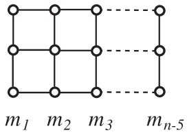
Figure 1: $A_{3}\times A_{n-5}$ diagram of the TBA system for the $n$-cusp minimal surfaces in AdS₄.

3.1 Perturbed unitary diagonal coset/$W$ minimal models

When only one mass parameter is turned on, $M_{s}=\delta_{s,r}M$, one expects from the AdS₃ case that the TBA system of the HSG model reduces to that for the unitary

$$\mathrm{SU}(4)_{r}\times\mathrm{SU}(4)_{n-4-r}/\mathrm{SU}(4)_{n-4}$$ (3.1)

diagonal coset model perturbed by $\phi_{(1,1,{\rm adj})}$ with dimension $h_{(1,1,{\rm adj})}=\bar{h}_{(1,1,{\rm adj})}=(n-4)/n$. In particular, when $r=1$, the above model becomes equivalent to the perturbed unitary $W$ minimal model,

$$WA_{3}^{(n-1,n)}\,.$$ (3.2)

Here, we have used the relations (3.11) and (3.12).

This expectation is also supported by an observation that the TBA system of the $\mathrm{SU}(N)$ Gross-Neveu model, which is characterized by the $A_{N-1}\times A_{m}$ diagram with $m\to\infty$, is given by the TBA system of the perturbed $\mathrm{SU}(N)_{1}\times\mathrm{SU}(N)_{m}/\mathrm{SU}(N)_{1+m}$ diagonal coset model [45]. Indeed, one can explicitly check that the above correspondences of the TBA systems are correct by comparing the TBA equations of the HSG model and those of the $\mathrm{G}_{k}\times\mathrm{G}_{k}/\mathrm{G}_{k+l}$ diagonal coset model perturbed by $\phi_{(1,1,{\rm adj})}$ [46].

3.2 Perturbed non-unitary diagonal coset/$W$ minimal models

When a pair of the mass parameters are turned on, $M_{s}=(\delta_{s,r}+\delta_{s,n-4-r})M$, with $n$ odd, the TBA system is characterized by the diagram $(A_{3}\times T_{(n-5)/2})_{r}$, namely, the $A_{3}\times T_{(n-5)/2}$ diagram with a mass parameter only for the $r^{\rm th}$ column. Taking into account the above and AdS₃ cases, one then expects that the TBA system in this case reduces to that for the non-unitary

$$\mathrm{SU}(4)_{r}\times\mathrm{SU}(4)_{n/2-4-r}/\mathrm{SU}(4)_{n/2-4}$$ (3.3)

diagonal coset model perturbed by $\phi_{(1,1,{\rm adj})}$ with dimension $h_{(1,1,{\rm adj})}=\bar{h}_{(1,1,{\rm adj})}=(n-8)/n$. The relation $1-h_{(1,1,{\rm adj})}=2(1-\Delta)$ is consistent with the UV expansion. In particular, when $r=1$, this perturbed diagonal coset model becomes equivalent to the perturbed non-unitary $W$ minimal model,

$$WA_{3}^{(n-2,n)}\,.$$ (3.4)

These are particular examples of the correspondence between the TBA system characterized by the diagram $(\mathrm{G}\times T_{l})_{r}$ and the non-unitary diagonal coset model for $\mathrm{G}$, which has been suggested in [47]. In the following sections, assuming, in particular, the correspondence for the 7-cusp ($n=7$) case, we derive the analytic expansion of the remainder function around the UV limit, to find a good agreement with the results from the numerical computation. We regard this also as a non-trivial check of the above correspondence.

3.3 $W$ minimal models

In the previous subsections, we observed/argued that the TBA systems for the AdS₄ minimal surfaces in the single-mass cases reduce to those for the diagonal coset/$W$ minimal models. As mentioned, we consider the cases corresponding to the $W$ minimal models to determine the UV expansion of the remainder function for $n=6$ and $7$. For later use, we thus summarize the $W$ minimal model below.

In the following, we focus on the $WA_{k-1}^{(p,q)}$ minimal model [48], where $p,q$ ($p<q$) are positive and relatively prime integers. The central charge of the model is

$$c(WA_{k-1}^{(p,q)})=(k-1)\left(1-{k(k+1)(p-q)^{2}\over pq}\right)\,.$$ (3.5)

The primary fields $\Phi_{l,l^{\prime}}$ have the dimensions

$$h_{l,l^{\prime}}={12\boldsymbol{\Lambda}_{l,l^{\prime}}^{2}-k(k^{2}-1)(p-q)^{2}\over 24pq}\,.$$ (3.6)

Here, $l=(l_{1},\cdots,l_{k-1})$ and $l^{\prime}=(l^{\prime}_{1},\cdots,l^{\prime}_{k-1})$ are vectors of positive integers satisfying

$$\sum_{i=1}^{k-1}l_{i}\leq q-1,\quad\sum_{i=1}^{k-1}l^{\prime}_{i}\leq p-1\,.$$ (3.7)

$\boldsymbol{\Lambda}_{l,l^{\prime}}$ is given by

$$\boldsymbol{\Lambda}_{l,l^{\prime}}=\sum_{i=1}^{k-1}(pl_{i}-ql^{\prime}_{i})\boldsymbol{\omega}_{i}\,,$$ (3.8)

where $\boldsymbol{\omega}_{i}$ ($i=1,\cdots,k-1$) are the fundamental weights of $A_{k-1}$ normalized as

$$\boldsymbol{\omega}_{i}\cdot\boldsymbol{\omega}_{j}={i(k-j)\over k}\quad{\rm for}\quad i\leq j\,.$$ (3.9)

We also define the effective central charge by $c_{\rm eff}(WA_{k-1}^{(p,q)}):=c(WA^{(p,q)}_{k-1})-24h_{0}$, where $h_{0}$ denotes the lowest conformal weight. For the unitary model with $q=p+1$, the lowest weight is 0, but otherwise it is evaluated as [49]

$$c_{\rm eff}(WA_{k-1}^{(p,q)})=(k-1)\left(1-{k(k+1)\over pq}\right)\,.$$ (3.10)

The $WA_{k-1}^{(p,q)}$ minimal model is represented by the coset model as [50]

$$WA_{k-1}^{(p,q)}={\mathrm{SU}(k)_{1}\times\mathrm{SU}(k)_{m}\over\mathrm{SU}(k)_{1+m}}\,,$$ (3.11)

where

$$m+k=\frac{p}{q-p}\,.$$ (3.12)

We note that $m$ is not generally a non-negative integer corresponding to an integrable representation. Instead, the general $m$ corresponds to an admissible representation. Let $(\boldsymbol{\mu}_{1},\boldsymbol{\mu}_{m},\boldsymbol{\mu}_{m+1})$ be the weighs of $\mathfrak{su}(k)$ for $\mathrm{SU}(k)_{1},\mathrm{SU}(k)_{m}$ and $\mathrm{SU}(k)_{m+1}$, respectively. Since $\boldsymbol{\mu}_{1}$ is determined by other two weights [49, 50, 51], one can label the fields in the coset model by

$$(\boldsymbol{\Lambda}_{+},\boldsymbol{\Lambda}_{-}):=(\boldsymbol{\mu}_{m},\boldsymbol{\mu}_{m+1})\,.$$ (3.13)

Then, the dimension of the field is given by

$$h_{(\boldsymbol{\Lambda}_{+},\boldsymbol{\Lambda}_{-})}={\bigl{[}q\boldsymbol{\Lambda}_{+}-p\boldsymbol{\Lambda}_{-}+(q-p)\boldsymbol{\rho}\bigr{]}^{2}-(q-p)^{2}\boldsymbol{\rho}^{2}\over 2pq}\,,$$ (3.14)

where $\boldsymbol{\rho}$ is the Weyl vector of $\mathfrak{su}(k)$, i.e.,

$$\boldsymbol{\rho}=\sum_{i=1}^{k-1}\boldsymbol{\omega}_{i}\,.$$ (3.15)

Since $\boldsymbol{\rho}^{2}=k(k^{2}-1)/12$, comparing (3.14) and (3.6) gives

$$\pm\boldsymbol{\Lambda}_{l,l^{\prime}}=q\boldsymbol{\Lambda}_{+}-p\boldsymbol{\Lambda}_{-}+(q-p)\boldsymbol{\rho}\,,$$ (3.16)

up to field identifications.

For example, the perturbing operator $\phi_{(1,1,{\rm adj})}$ for the single-mass cases is labeled by

$$(\boldsymbol{\Lambda}_{+},\boldsymbol{\Lambda}_{-})=(0,\boldsymbol{\omega}_{1}+\boldsymbol{\omega}_{k-1})\,,$$ (3.17)

and has the dimension

$$h_{\rm(1,1,adj)}=\frac{p-(k-1)(q-p)}{q}=\frac{m+1}{m+k+1}\,.$$ (3.18)

In addition, for the non-unitary model $WA_{3}^{(n-2,n)}$ with $n$ odd, which is used later, the vacuum or ground-state operator $\phi_{0}$ is labeled by

$$(\boldsymbol{\Lambda}_{+},\boldsymbol{\Lambda}_{-})=\Bigl{(}\frac{n-7}{2}\boldsymbol{\omega}_{2},\frac{n-5}{2}\boldsymbol{\omega}_{2}\Bigr{)}\,,$$ (3.19)

and has the dimension

$$h_{0}=-{15\over 2n(n-2)}\,.$$ (3.20)

The effective central charge is then $c_{\rm eff}=3\bigl{(}1-{20\over n(n-2)}\bigr{)}\,.$

3.4 Level-rank duality and decomposition of coset models

In subsection 3.1, we discussed the relation between the TBA systems of the HSG model in the single-mass cases and those of the perturbed unitary $W$ minimal models. This relation is directly found by using a decomposition of the generalized parafermion model into a product of the diagonal coset models based on the level-rank duality [52, 53].

Let us start with a simple example of the $\mathrm{SU}(2)_{k}/\mathrm{U}(1)$ coset or the ${\mathbb{Z}}_{k}$-parafermion theory [54, 55], which has the central charge $c=2(k-1)/(k+2)$ according to (2.16). The perturbing operator, i.e., weight-zero adjoint operator, has the conformal dimension $2/(k+2)$. By the level-rank duality, this parafermion CFT is equivalent to the $\mathrm{SU}(k)_{1}\times\mathrm{SU}(k)_{1}/\mathrm{SU}(k)_{2}$ diagonal coset CFT or the $WA_{k-1}^{(k+1,k+2)}$ minimal model which has the same central charge [56]. The perturbing field on the dual side is $\phi_{(1,1,{\rm adj})}$ with the dimension (3.18) for $m=1$, which indeed coincides with $2/(k+2)$.

The above equivalence between the perturbed parafermion and diagonal coset/$W$ minimal models can be generalized to the case of $\mathrm{SU}(N)_{k}/\mathrm{U}(1)^{N-1}$. We see that

$${\mathrm{SU}(N)_{k}\over\mathrm{U}(1)^{N-1}} = {(\mathrm{SU}(k)_{1})^{N}\over\mathrm{SU}(k)_{N}}$$ (3.21)

$$= {\mathrm{SU}(k)_{1}\times\mathrm{SU}(k)_{1}\over\mathrm{SU}(k)_{2}}\times{\mathrm{SU}(k)_{1}\times\mathrm{SU}(k)_{2}\over\mathrm{SU}(k)_{3}}\times\cdots\times{\mathrm{SU}(k)_{1}\times\mathrm{SU}(k)_{N-1}\over\mathrm{SU}(k)_{N}}\,.\quad$$

The first equation is due to [57], and the second expression is due to [58]. The matching of the central charges follows from

$$c({\mathrm{SU}(N)_{k}\over\mathrm{U}(1)^{N-1}})-c({\mathrm{SU}(N-1)_{k}\over\mathrm{U}(1)^{N-2}})=c(WA_{k-1}^{(k+N-1,k+N)}).$$ (3.22)

In the decomposition (3.21), the dimension of the perturbing operator on the left-hand side is $\Delta=N/(N+k)$, which coincides with that of $\phi_{(1,1,{\rm adj})}$ in the rightmost model on the right-hand side. This means that a weight-zero operator on the l.h.s. is represented solely by the $\phi_{(1,1,{\rm adj})}$ operator in the rightmost model, and thus the corresponding single-mass case is described by the ${\mathrm{SU}(k)_{1}\times\mathrm{SU}(k)_{N-1}/\mathrm{SU}(k)_{N}}=WA_{k-1}^{(N+k-1,N+k)}$ model perturbed by $\phi_{(1,1,{\rm adj})}$.

For example, for the level $k=2$ corresponding to the AdS₃ case, one has a product of the unitary minimal models in (3.21), and the relation has also been confirmed by the decomposition of the characters [59, 60]. Further setting $N=\tilde{n}-2$ for the $2\tilde{n}$-cusp minimal surfaces, the rightmost model becomes the unitary ${\cal M}_{\tilde{n}-1,\tilde{n}}$ minimal model, as already discussed. For $k=4$ and $N=n-4$, we indeed have the unitary $WA_{3}^{(n-1,n)}$ minimal model.

One finds a similar “decomposition” also for the TBA system characterized by the $A_{k-1}\times T_{(N-1)/2}$ diagram with $N$ odd. To see this, we first note the relation among the central charges,

$$c({\mathrm{SU}(N)_{k}\over\mathrm{U}(1)^{N-1}})-c({\mathrm{SU}(N-2)_{k}\over\mathrm{U}(1)^{N-3}})=2c_{\rm eff}(WA_{k-1}^{(k+N-2,k+N)})\,,$$ (3.23)

and then denote the relation after a successive use of it by

$${\mathrm{SU}(N)_{k}\over\mathrm{U}(1)^{N-1}}\sim(WA_{k-1}^{(k+1,k+3)})^{2}\star(WA_{k-1}^{(k+3,k+5)})^{2}\star\cdots\star(WA_{k-1}^{(k+N-2,k+N)})^{2}.$$ (3.24)

In parallel with the decomposition (3.21), we find that the rightmost factor on the r.h.s., $WA_{k-1}^{(k+N-2,k+N)}={\mathrm{SU}(k)_{1}\times\mathrm{SU}(k)_{(k+N)/2-k-1}/\mathrm{SU}(k)_{(k+N)/2-k}}$, is the non-unitary diagonal coset/$W$ minimal model describing the TBA system in the single-mass case which is characterized by $(A_{k-1}\times T_{(N-1)/2})_{1}$. In particular, for the $n$-cusp minimal surfaces in AdS₄ with $n$ odd, we have $WA_{3}^{(n-2,n)}={\mathrm{SU}(4)_{1}\times\mathrm{SU}(4)_{n/2-5}/\mathrm{SU}(4)_{n/2-4}}$, as already observed in subsection 3.2.

We note that, in the rank 2 cases with $N=3$, there is only one factor of $(WA_{k-1}^{(k+1,k+3)})^{2}$ on the r.h.s. of (3.24), which means that the central charge of the model on the l.h.s. is twice that on the r.h.s.. This is in accord with the fact that the free energy for the $A_{k-1}\times A_{2}$ TBA system with equal mass parameters is twice that for $(A_{k-1}\times T_{1})_{1}$ (see the next section). Explicitly, in the AdS₃ case with $\tilde{n}=N+2=5$, the relation (3.24) reads as ${\mathrm{SU}(3)_{2}/\mathrm{U}(1)^{2}}\sim(WA_{1}^{(3,5)})^{2}=({\cal M}_{3,5})^{2}$. This was used to determine the UV expansion of the remainder function for the 10-cusp minimal surfaces [26]. In the next section, we use the relation for the AdS₄ case with $n=N+4=7$,

$${\mathrm{SU}(3)_{4}\over\mathrm{U}(1)^{3}}\sim(WA_{3}^{(5,7)})^{2}\,,$$ (3.25)

to determine the UV expansion for the 7-cusp minimal surfaces.

The “decomposition” (3.24) based on the counting of the central charges tells us which $W$ minimal model appears in the single-mass case. It would be of interest to substantiate this relation at a more fundamental level.

4 UV expansion of free energy

As explained in section 2, the HSG model is regarded as an integrable perturbation of the generalized parafermion theory. Near the UV fixed point, we can thus analyze it by using the 2d CFT technique. In this section, we consider the UV expansion of the free energy for the $\mathrm{SU}(n-4)_{4}/\mathrm{U}(1)^{n-5}$ HSG model. In particular, we write down the analytic expression of the UV expansion for $n=6,7$. The connection between the generalized parafermions and the $W$ minimal models in the previous section is useful. The expansion of the T-functions will be considered in the next section. Before proceeding to detailed analysis, we note our notation for the mass parameters:

$$m_{s}=M_{s}L=\tilde{M}_{s}l,\qquad l=ML,$$ (4.1)

where $\tilde{M}_{s}$ are the relative masses, $M$ is the overall mass scale, and $L$ is the circumference of the cylinder on which the HSG model is defined.

Since the weight-zero adjoint operators of the $\mathrm{SU}(n-4)_{4}/\mathrm{U}(1)^{n-5}$ generalized parafermion theory have the dimension $\Delta=\bar{\Delta}=(n-4)/n$, the free energy is expanded around the UV fixed point $l=0$ as [17]

$$A_{\rm free}=\frac{\pi}{6}c_{n}+f_{n}^{\rm bulk}+\sum_{p=2}^{\infty}f_{n}^{(p)}l^{8p/n},$$ (4.2)

where $c_{n}$ is the central charge and $f_{n}^{\rm bulk}$ is the bulk contribution. In the case of our interest, $\mathrm{SU}(n-4)_{4}/\mathrm{U}(1)^{n-5}$, the central charge is given by

$$c_{n}=\frac{3(n-4)(n-5)}{n}.$$ (4.3)

The general form of the bulk term is not known. Here we assume, as in the AdS₃ case [26, 27], that this term just cancels the period term $A_{\rm periods}$ around the UV limit, i.e.,

$$f_{n}^{\rm bulk}=-A_{\rm periods}.$$ (4.4)

This is equivalent to requiring that the remainder function is expanded by $l^{4p/n}$ for $n\notin 4{\mathbb{Z}}$, as is the case for the T-/Y-functions discussed in the next section. For $n=6$, this is indeed the case [22], and we argue below that this holds also for $n=7$. We expect it to be true for any $n\not\in 4\mathbb{Z}$.

The expansion coefficients $f_{n}^{(p)}$ are obtained from the connected $n$-point correlation functions of the perturbing operator $\Phi$ at the CFT point. In particular, $f_{n}^{(2)}$ is given by

$$f_{n}^{(2)}=\frac{\pi}{6}(\kappa_{n}G(\tilde{M}_{s}))^{2}C_{n}^{(2)},$$ (4.5)

where we have denoted the dimensionless coupling in (2.20) by $\kappa_{n}$. The function $G(\tilde{M}_{s})$ is introduced as the normalization of the two-point function of the perturbing operator $\Phi$ in (2.18) parametrized by $\tilde{M}_{s}$,

$$\langle\Phi(z)\Phi(0)\rangle=\frac{G^{2}(\tilde{M}_{s})}{|z|^{4\Delta}},$$ (4.6)

and $C_{n}^{(2)}$ is given by

$$C_{n}^{(2)}=3(2\pi)^{2-16/n}\gamma^{2}\left(1-\frac{4}{n}\right)\gamma\left(\frac{8}{n}-1\right),$$ (4.7)

with $\gamma(x)=\Gamma(x)/\Gamma(1-x)$. We still need to determine the function $G(\tilde{M}_{s})$. As discussed below, it is trivial for $n=6$, whereas for $n=7$ it is determined by using the relation between the TBA system and the $W$ minimal models in the previous section.

4.1 Case of six-cusp minimal surfaces ($n=6$)

In this case, there is only one mass scale. Thus the above function is trivially given by $G(\tilde{M}_{1})=\tilde{M}_{1}$, which is equal to 1 for real $m_{1}$. As discussed in the previous section, the HSG model for $n=6$ is equivalent to a perturbed ${\mathbb{Z}}_{4}$-parafermion or $\mathrm{SU}(4)_{1}\times\mathrm{SU}(4)_{1}/\mathrm{SU}(4)_{2}=WA_{3}^{(5,6)}$ model. The constant $\kappa_{6}$ is thus read from the exact mass-coupling relation in [61]

$$\kappa_{6}G=\frac{1}{2\pi}\gamma^{1/2}\left(\frac{1}{6}\right)\left[\sqrt{\pi}\gamma\left(\frac{3}{4}\right)\right]^{4/3}.$$ (4.8)

We thus obtain

$$f_{6}^{(2)}=\frac{\pi}{6}\kappa_{6}^{2}G^{2}C_{6}^{(2)}=\frac{\pi}{2}\gamma^{3}\left(\frac{1}{3}\right)\gamma\left(\frac{1}{6}\right)\left[\frac{1}{2\sqrt{\pi}}\gamma\left(\frac{3}{4}\right)\right]^{\frac{8}{3}}.$$ (4.9)

This is indeed obtained by setting $\mu=1$ in the results in [26]. As discussed in [26], this expression is continued to the complex-mass case as $G^{2}(\tilde{M}_{s})\to|G(\tilde{M}_{s}e^{i\varphi_{s}})|^{2}$ so as to maintain the ${\mathbb{Z}}_{n}$-symmetry. The continuation in this case is, however, trivial, to give $|G|^{2}=1$.

4.2 Case of seven-cusp minimal surfaces ($n=7$)

In this case, there are two mass parameters $(m_{1},m_{2})$, which we first set to be real. To fix the function $G(\tilde{M}_{1},\tilde{M}_{2})$, we use the strategy explained in the previous section (see also [26]). From the symmetry and the dimensional analysis, we see that this function takes the form

$$G(\tilde{M}_{1},\tilde{M}_{2})=\sum_{r,s=1}^{2}F_{rs}\tilde{M}_{r}^{4/7}\tilde{M}_{s}^{4/7},$$ (4.10)

where $F_{11}=F_{22}$ and $F_{12}=F_{21}$. We would like to fix such coefficients. For this purpose, we consider the following two cases.

Let us first consider the case where $(m_{1},m_{2})\to(l,0)$. In this case, the TBA equations reduce to those for an integrable perturbation of the $W$ minimal model,

$$WA_{3}^{(6,7)}=\mathrm{SU}(4)_{1}\times\mathrm{SU}(4)_{2}/\mathrm{SU}(4)_{3}.$$ (4.11)

The perturbing operator is the relevant operator $\Phi$ with dimension $\Delta=\bar{\Delta}=3/7$. The bulk term in this TBA system is [62]

$$f^{\rm bulk}=-\frac{1}{2}l^{2}\,.$$ (4.12)

We can also read off the mass-coupling relation for this perturbed model from [61]:

$$\kappa_{7}G(1,0)=\kappa_{7}F_{11}=\frac{2}{3\pi}\left[\gamma\left(\frac{2}{7}\right)\gamma\left(\frac{4}{7}\right)\right]^{1/2}\left[\frac{3}{4\sqrt{2}}\Gamma^{2}\left(\frac{3}{4}\right)\right]^{8/7}.$$ (4.13)

To fix $F_{12}$, let us next consider the case with $m_{1}=m_{2}$. As argued in the previous section, the TBA equations in this case may be equivalent to those for an integrable perturbation of the non-unitary $W$ minimal model,

$$WA_{3}^{(5,7)}=\mathrm{SU}(4)_{1}\times\mathrm{SU}(4)_{-3/2}/{\rm SU(4)}_{-1/2}.$$ (4.14)

The central charge and the effective central charge of this CFT are given, respectively, by

$$c(WA_{3}^{(5,7)})=-\frac{27}{7},\qquad c_{\rm eff}(WA_{3}^{(5,7)})=\frac{9}{7}.$$ (4.15)

The perturbing operator $\hat{\Phi}=\phi_{(1,1,{\rm adj})}$ labeled by the weight (3.17) has the conformal dimension $\hat{\Delta}=\bar{\hat{\Delta}}=-1/7$, while the vacuum operator $\hat{\Phi}_{0}=\phi_{0}$ labeled by (3.19) has the dimension $\Delta_{0}=\bar{\Delta}_{0}=-{3}/{14}$.

Now, let us consider the UV expansion of the free energy for this TBA system. The mass-coupling relation [61] reads as

$$\hat{\lambda}=\hat{\kappa}M^{32/7},$$ (4.16)

where

$$(\pi\hat{\kappa})^{2}=9\gamma\left(\frac{1}{7}\right)\gamma\left(-\frac{3}{7}\right)\left[\frac{\Gamma(\frac{3}{4})\Gamma(\frac{7}{8})}{2\Gamma(\frac{5}{8})}\right]^{\frac{32}{7}}.$$ (4.17)

The free energy is expanded around the UV fixed point as

$$\hat{F}(l)=\frac{\pi}{6}c_{\rm eff}+\hat{f}^{\rm bulk}(l)+\sum_{p=1}^{\infty}\hat{f}^{(p)}l^{16p/n},$$ (4.18)

where the bulk term is given by [62]

$$\hat{f}^{\rm bulk}(l)=-\frac{1+\sqrt{2}}{2\sqrt{2}}l^{2},$$ (4.19)

and the coefficients $\hat{f}^{(p)}$ are expressed as

$$\hat{f}^{(p)}=\frac{\pi}{6}\hat{\kappa}^{p}\hat{C}^{(p)}.$$ (4.20)

The coefficients $\hat{C}^{(p)}$ are given by the correlation functions of the vacuum and the perturbing operators, and the integral forms of $\hat{C}^{(p)}$ are found in [17, 63]. Here, we are interested in the first correction given by

$$\hat{f}^{(1)}=\frac{\pi}{6}\hat{\kappa}\hat{C}^{(1)},\qquad\hat{C}^{(1)}=-12(2\pi)^{2\hat{\Delta}-1}C_{\hat{\Phi}_{0}\hat{\Phi}\hat{\Phi}_{0}},$$ (4.21)

where $C_{\hat{\Phi}_{0}\hat{\Phi}\hat{\Phi}_{0}}$ is the three-point structure constant. This structure constant is computed in Appendix A, and given by (A.20). Thus the first correction is finally given by

$$\hat{f}^{(1)}=\frac{1}{2\pi^{9/7}}\gamma\left(\frac{2}{7}\right)\gamma\left(\frac{1}{14}\right)\left[\frac{\Gamma(\frac{3}{4})\Gamma(\frac{7}{8})}{2\Gamma(\frac{5}{8})}\right]^{\frac{16}{7}}.$$ (4.22)

From this result, we can fix $F_{12}$. For $m_{1}=m_{2}$ ($\tilde{M}_{1}=\tilde{M}_{2}=1$), we find from (4.10) that

$$f_{7}^{(2)}=\frac{\pi}{6}(\kappa_{7}F_{11})^{2}C_{7}^{(2)}\times 4\left(1+\frac{F_{12}}{F_{11}}\right)^{2}.$$ (4.23)

This correction must be twice $\hat{f}^{(1)}$. Using (4.7), (4.13) and (4.22), we thus obtain

$$1+\frac{F_{12}}{F_{11}}=\left(\frac{\pi^{8}}{2^{3}\cdot 3^{2}}\right)^{\frac{1}{14}}\left[\gamma\left(\frac{4}{7}\right)\gamma\left(\frac{6}{7}\right)\gamma\left(\frac{1}{14}\right)\right]^{1/2}\left[\frac{\Gamma(\frac{7}{8})}{\Gamma(\frac{3}{4})\Gamma(\frac{5}{8})}\right]^{\frac{8}{7}}.$$ (4.24)

In summary, for $n=7$, the function $G(\tilde{M}_{1},\tilde{M}_{2})$ has the following form,

$$\kappa_{7}G(\tilde{M}_{1},\tilde{M}_{2})=\kappa_{7}F_{11}(\tilde{M}_{1}^{8/7}+\tilde{M}_{2}^{8/7}+B\tilde{M}_{1}^{4/7}\tilde{M}_{2}^{4/7}),$$ (4.25)

where $\kappa_{7}F_{11}$ is given by (4.13) and the constant $B$ is given by

$$B=\left(\frac{2^{11}\pi^{8}}{3^{2}}\right)^{\frac{1}{14}}\left[\gamma\left(\frac{4}{7}\right)\gamma\left(\frac{6}{7}\right)\gamma\left(\frac{1}{14}\right)\right]^{1/2}\left[\frac{\Gamma(\frac{7}{8})}{\Gamma(\frac{3}{4})\Gamma(\frac{5}{8})}\right]^{\frac{8}{7}}-2.$$ (4.26)

We also find that the bulk terms in the above two cases, (4.12) and (4.19), fix the form in the general case to be $f^{\rm bulk}(l)=-A_{\rm periods}$, as expected. Thus, from the connections to the $W$ minimal models, we indeed find this relation for $n=7$.

So far, we have considered the case of real $m_{s}$. Let us now consider the UV expansion of the free energy when the masses are complex. By the relation to $A_{\rm periods}$, or the argument in [26] to maintain the ${\mathbb{Z}}_{n}$-symmetry, the bulk term is given by

$$f^{\rm bulk}(l) =-A_{\rm periods}=-\frac{1}{2}(m_{1}\bar{m}_{1}+m_{2}\bar{m}_{2})-\frac{1}{2\sqrt{2}}(m_{1}\bar{m}_{2}+m_{2}\bar{m}_{1})$$

$$=-\frac{1}{2}\left(\tilde{M}_{1}^{2}+\tilde{M}_{2}^{2}+\sqrt{2}\tilde{M}_{1}\tilde{M}_{2}\cos(\varphi_{1}-\varphi_{2})\right)l^{2},$$ (4.27)

where $|m_{s}|=\tilde{M}_{s}l$. Similarly, following [26], we find that the function $G$ is continued as

$$G^{2}(\tilde{M}_{1},\tilde{M}_{2})\to|G(\tilde{M}_{1}e^{i\varphi_{1}},\tilde{M}_{2}e^{i\varphi_{2}})|^{2}.$$ (4.28)

In order to check the validity of these expressions, we compare them with numerical results from the TBA equations. Here, we remark that the TBA equations for the AdS₄ minimal surfaces generally exhibit an instability [64] around the UV limit, in that simple iterations for numerics do not converge. However, we have found that numerics based on the iteration works if $|m_{1}|=|m_{2}|$ up to some value of $l$. When the phases are turned off, the numerics works for smaller $l$. For the comparison, we have thus solved the TBA equations for $|m_{1}|=|m_{2}|$ from $l=1/20$ to $l=1/2$ with step $1/100$ for various values of $\varphi:=\varphi_{1}-\varphi_{2}$. We have then fitted the free energy by the function,

$$A_{\rm free}^{(\rm fit)}=\frac{\pi}{6}c+bl^{2}+f_{7}^{(2)}l^{16/7}+f_{7}^{(3)}l^{24/7}+f_{7}^{(4)}l^{32/7},$$ (4.29)

and found the best values of the fitting for each value of $\varphi$. Note that $\tilde{Y}_{a,s}$ and hence $A_{\rm free}$ depend on the phases only through $\varphi$ in this case. In Fig. 2, we plot the $\varphi$-dependence of the coefficients $b$ and $f_{7}^{(2)}$. The solid lines represent our analytic prediction while the dots show the numerical data from the TBA equations. Our analytic expressions show a good agreement with the numerical data, which strongly supports the correspondence to the non-unitary $W$ minimal models proposed in subsection 3.2, as well as the continuation to the complex masses.

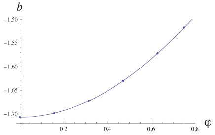
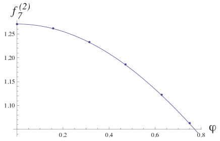
Figure 2: The (relative) phase dependence of the bulk term (left) and $f_{7}^{(2)}$ (right).

5 UV expansion of T-functions

To derive the UV expansion of the remainder function, we need to expand the Y-/T-functions, as well as the free energy part discussed in the previous section. This is achieved by using an interesting relation between the T-function and the $g$-function (boundary entropy) [65, 18]. Here, we extend the discussion for the minimal surfaces in AdS₃ [26, 27] to the AdS₄ case. We concentrate on the case with $n\notin 4{\mathbb{Z}}$.

5.1 T-functions for $\mathrm{SU}(N)_{4}/\mathrm{U}(1)^{N-1}$ HSG model

The first step to derive the expansion of $T_{a,s}$ is to compare the integral equations for the $T$- and $g$-functions of the $\mathrm{SU}(N)_{k}/\mathrm{U}(1)^{N-1}$ HSG model with level $k=4$. In this subsection, we consider those for the T-functions, which are obtained by a procedure similar to the one from Y-systems to TBA equations. The extension to general $k$ may be straightforward. For the reason explained in the next subsection, we also set $m_{s}$ to be real.

Let us start our discussion by considering the asymptotic behavior of $T_{a,s}$ for large $|\theta|$. To see this, we note that, when $N\in 2{\mathbb{Z}}+1$ with the boundary conditions (2.2), (2.3), one can invert the relation between the Y- and T-functions (2.4) for AdS₅, to express $T_{a,s}$ by $Y_{a,s}$. This is also possible for $N\in 4{\mathbb{Z}}+2$ after imposing the AdS₄ condition $Y_{1,s}=Y_{3,s}$ and $T_{1,s}=T_{3,s}$. In such cases, the asymptotic behavior of $Y_{a,s}$ (2.1) implies that of $T_{a,s}$,

$$\log T_{a,s}\to-\nu_{a,s}\cosh\theta\,,$$ (5.1)

for $0\leq a\leq k(=4)$ and $0\leq s\leq N$, where constants $\nu_{a,s}$ are related by (2.4) to $m_{a,s}=M_{a,s}L$ as

$$m_{a,s}=\nu_{a,s+1}+\nu_{k-a,s-1}-\nu_{a+1,s}-\nu_{a-1,s}\,.$$ (5.2)

At the boundary $a=0,k$ or $s=0,N$, we have $\nu_{a,s}=0$. The above relation together with the mass ratios (2.21) in turn gives

$$\nu_{a,s}=\nu_{s}\sin\bigl{(}\frac{\pi a}{k}\bigr{)}/\sin\bigl{(}\frac{\pi}{k}\bigr{)}\,,$$ (5.3)

and hence

$$m_{s}=\bigl{(}I_{N-1}-2\cos\frac{\pi}{k}\cdot{\bf 1}\bigr{)}_{sr}\nu_{r}\,,$$ (5.4)

where ${\bf 1}$ is the $(N-1)\times(N-1)$ unit matrix and $I_{N-1}$ is the incidence matrix for $A_{N-1}$. This relation is inverted as

$$\nu_{s}=(V_{N-1}\cdot J_{N-1}\cdot V_{N-1})_{sr}m_{r}\,,$$ (5.5)

where

$$(V_{N-1})_{rs}:=\sqrt{\frac{2}{N}}\sin\frac{rs\pi}{N}\,,$$ (5.6)

and $(J_{N-1})_{rs}:={\delta_{rs}}/{2(\cos\frac{\pi r}{N}-\cos\frac{\pi}{k})}$. We have also used $V_{N-1}^{-1}=V_{N-1}$ and

$$(V_{N-1}\cdot I_{N-1}\cdot V_{N-1})_{rs}=\delta_{rs}\cdot 2\cos\frac{\pi r}{N}\,.$$ (5.7)

Given the asymptotics (5.1) , we next subtract the linear terms in $l=ML$ from $\log T_{a,s}$ and define

$$U_{a,s}:=\log(T_{a,s}e^{\nu_{a,s}\cosh\theta})\,,$$ (5.8)

so that $U_{a,s}\to 0$ for large $|\theta|$. From (5.3) as well as the T-system (2.1) and the relation between $T_{a,s}$ and $Y_{a,s}$ (2.4) with $T_{k-a,s}=T_{a,s}$, we find that

$$\log\frac{T_{a,s}^{+}T_{a,s}^{-}}{T_{a+1,s}T_{a-1,s}}=U_{a,s}^{+}+U_{a,s}^{-}-U_{a+1,s}-U_{a-1,s}=\log(1+Y_{a,s})\,.$$ (5.9)

Note that terms with $\nu_{a,s}$ cancel each other due to (5.3), and that the above relation involves the same $s$ only. Assuming that $U_{a,s}$ are analytic in the strip $-\pi/k<\operatorname{Im}\theta<\pi/k$ and vanishing rapidly enough for large $|\theta|$, which is expected from the relation to $Y_{a,s}$, one can Fourier-transform the above equations. Further taking into account the boundary conditions on $T_{a,s}$ and using again (5.6) and (5.7) with $N$ being replaced by $k$, we obtain

$$\tilde{U}_{a,s}=-(V_{k-1}\cdot J^{\prime}_{k-1}\cdot V_{k-1})_{ab}\,\widetilde{\log(1+Y_{b,s})}\,,$$ (5.10)

where tildes stand for the Fourier transform, $\tilde{f}(\omega)=\int d\theta\,e^{i\omega\theta}f(\theta)$, and $J_{k-1}^{\prime}$ is given by $(J^{\prime}_{k-1})_{ab}:={\delta_{ab}}/{2(\cos\frac{\pi a}{k}-\cosh\frac{\pi\omega}{k})}$. Taking into account $U_{1,s}=U_{3,s}$ for $k=4$, and Fourier-transforming back (5.10), we find the integral equations of $U_{a,s}$ for $k=4$:

$$U_{a,s}={\cal K}_{ab}\ast\log(1+Y_{b,s})\,,$$ (5.11)

where

$${\cal K}(\theta)=\begin{pmatrix}K_{2}(\theta)&K_{1}(\theta)\\ 2K_{1}(\theta)&K_{2}(\theta)\end{pmatrix}\,,$$ (5.12)

and $K_{1},K_{2}$ are given in (2.9).

5.2 $g$-functions for $\mathrm{SU}(N)_{4}/\mathrm{U}(1)^{N-1}$ HSG model

Next, let us consider the $g$-function or boundary entropy for the $\mathrm{SU}(N)_{4}/\mathrm{U}(1)^{N-1}$ HSG model. The $g$-function is associated with a boundary, and hence with a set of corresponding reflection factors in an integrable quantum field theory. To keep the boundary integrability, we thus set the resonance parameters of the HSG model to be vanishing, so that the bulk S-matrix has the parity invariance up to constant factors $\eta_{r,s}$ in the S-matrix (2.22). This corresponds to considering real mass parameters $m_{s}$ in the TBA equations. The case of the complex $m_{s}$ is discussed later.

The reflection factors are constrained by the conditions from the unitarity, crossing-unitarity and boundary bootstrap [66, 67]. In our case, they read as

$$R_{a,s}(\theta)R_{a,s}(-\theta)=1\,,$$

$$R_{a,s}(\theta)R_{\bar{a},s}(\theta-i\pi)=S_{aa}^{ss}(2\theta)\,,$$ (5.13)

$$R_{\bar{c},s}(\theta)=R_{a,s}(\theta+i\bar{u}_{ac}^{b})R_{b,s}(\theta-i\bar{u}_{bc}^{a})S_{ab}^{ss}(2\theta+i\bar{u}_{ac}^{b}-i\bar{u}_{bc}^{a})\,.$$

Here, $\bar{u}=\pi-u$ and we have used $\overline{(a,s)}=(\bar{a},s)=(k-a,s)$. The location of the poles specified by $u^{a}_{bc}$ is the same as that for the $A_{k-1}$ minimal ATFT. Note that the boundary bootstrap equations involve the same label $s$ only. Given a set of the reflections factors $R_{a,s}$, one can deform it as $R^{\prime}_{a,s}=R_{a,s}/Z_{a,s}$ [68], where the deforming factors $Z_{a,s}$ need to satisfy

$$Z_{a,s}(\theta)Z_{a,s}(-\theta)=1\,,$$

$$Z_{a,s}(\theta)=Z_{\bar{a},s}(i\pi-\theta)\,,$$ (5.14)

$$Z_{\bar{c},s}(\theta)=Z_{a,s}(\theta+i\bar{u}_{ac}^{b})Z_{b,s}(\theta-i\bar{u}_{bc}^{a})\,,$$

in order to maintain the conditions (5.2).

Assuming the existence of the reflection factors corresponding to the boundary labeled by the identity operator, $R^{|\bf 1\rangle}_{a,s}$, we then consider the deformed reflection factors,

$$R_{a,s}^{|b,r;C\rangle}=R_{a,s}^{|{\bf 1}\rangle}/Z_{a,s}^{|b,r;C\rangle}\,,$$ (5.15)

where

$$Z_{a,s}^{|b,r;C\rangle}=\Bigl{[}S^{F}_{ab}\Bigl{(}\theta+\frac{i\pi}{k}C\Bigr{)}S^{F}_{ab}\Bigl{(}\theta-\frac{i\pi}{k}C\Bigr{)}\Bigr{]}^{\delta_{sr}}\,,$$ (5.16)

and $S_{ab}^{F}$ is defined in (2.25). The deforming factors $Z_{a,s}^{|b,r;C\rangle}$ are non-trivial only in the case $s=r$, where they reduce to those for the minimal ATFT [19]. This assures that they indeed satisfy the conditions (5.2). We also note that when $k=2$, the indices $a,b$ take only $1$, and the deforming factors of the form (5.16) reduce to

$$Z_{1,s}^{|1,r;C\rangle}=\Bigl{[}(1+C)_{\theta}(1-C)_{\theta}\Bigr{]}^{\delta_{sr}}\,,$$ (5.17)

which were used to analyze the T-functions for the minimal surfaces in AdS₃ [26, 27].

Given a pair of sets of the reflection factors, the $g$-functions associated with the corresponding boundaries satisfy [69, 19]

$$\log\frac{g_{|\alpha\rangle}(l)}{g_{|\beta\rangle}(l)}\frac{c_{|\beta\rangle}}{c_{|\alpha\rangle}}=\frac{1}{4}\sum_{\gamma}\int_{{\mathbb{R}}}d\theta\,\bigl{(}\phi_{\gamma}^{|\alpha\rangle}(\theta)-\phi_{\gamma}^{|\beta\rangle}(\theta)\bigr{)}\log\bigl{(}1+Y_{\gamma}(\theta)\bigr{)}\,,$$ (5.18)

where $c_{|\alpha\rangle}$ are certain constants related to the vacuum degeneracy, and

$$\phi_{\gamma}^{|\alpha\rangle}:=\frac{1}{\pi i}\partial_{\theta}\log R_{\gamma}^{|\alpha\rangle}(\theta)\,.$$ (5.19)

When we choose $R_{a,s}^{|b,r;C\rangle}$ and $R_{a,s}^{|{\bf 1}\rangle}$ for the pair, the right-hand side of (5.18) is determined only through the deforming factors $Z_{a,s}^{|b,r;C\rangle}$. By further using the relations $Y_{a,s}(\theta)=Y_{a,s}(-\theta)$ and $Y_{1,s}=Y_{3,s}$ for $k=4$, we find that

$$G_{a,s}(C):=\log\frac{g_{|a,s;C\rangle}(l)}{g_{|{\bf 1}\rangle}(l)}\frac{c_{|{\bf 1}\rangle}}{c_{|a,s;C\rangle}}=\Bigl{[}{\cal K}_{ab}\ast\log(1+Y_{b,s})\Bigr{]}\Bigl{(}\frac{i\pi}{k}C\Bigr{)}\,.$$ (5.20)

By comparing (5.11) and (5.20), we see that $G_{a,s}(C)=U_{a,s}\bigl{(}\frac{\pi i}{k}C\bigr{)}$. Moreover, assuming that $c_{|{\bf 1}\rangle}=c_{|a,s;C\rangle}$ as in the case of AdS₃, and subtracting the linear terms in $l\propto\nu_{a,s}$ from both sides, we arrive at the relation,

$$\frac{{\cal G}^{(0)}_{|a,s;C\rangle}}{{\cal G}^{(0)}_{|{\bf 1}\rangle}}=T_{a,s}\Bigl{(}\frac{\pi i}{k}C\Bigr{)}\,.$$ (5.21)

The ratios of ${\cal G}^{(0)}_{|\alpha\rangle}:=\log g_{|\alpha\rangle}-f_{|\alpha\rangle}l$ on the left-hand side, with $f_{|\alpha\rangle}$ being a constant, are the quantities which are directly computed around the UV limit by the conformal perturbation theory with boundaries [18, 19].

5.3 Expansion of $T_{a,s}$

Another input for the expansion of the T-functions is their periodicity. To see this, we first note that, from the Y-system (2.5) with $Y_{1,s}=Y_{3,s}$ and the boundary conditions given in section 2.1, the Y-functions have the quasi-periodicity,

$$Y_{a,s}\Bigl{(}\theta+\frac{n}{k}\pi i\Bigr{)}=Y_{a,N-s}(\theta)\,,$$ (5.22)

where $n=N+k$ and $k=4$. Since our T-functions are expressed by the Y-functions for $N\notin 4{\mathbb{Z}}$, they inherit the same quasi-periodicity,

$$T_{a,s}\Bigl{(}\theta+\frac{n}{k}\pi i\Bigr{)}=T_{a,N-s}(\theta)\qquad(N\notin 4{\mathbb{Z}})\,.$$ (5.23)

Taking also into account the structure of the CPT, we find that $T_{a,s}$ are expanded as

$$T_{a,s}(\theta)=\sum_{p,q=0}^{\infty}t^{(p,2q)}_{a,s}l^{(1-\Delta)(p+2q)}\cosh\Bigl{(}\frac{kp}{n}\theta\Bigr{)}\,,$$ (5.24)

with $t_{a,N-s}^{(p,2q)}=(-1)^{p}t_{a,s}^{(p,2q)}$. For lower orders, one can check from the T-system (2.1) that the terms $t_{a,s}^{p,q^{\prime}}$ with $q^{\prime}$ odd are indeed absent, and that the first two non-trivial coefficients are $t_{a,s}^{(0,0)}$ and $t_{a,s}^{(2,0)}$. The Y-functions also have similar expansion, the coefficients of which are related to $t_{a,s}^{(p,2q)}$ by (2.4) with (2.10).

To compute these coefficients using the relation to the $g$-functions (5.21), we still need to find which boundary the reflection factors $R_{a,s}^{|b,r;C\rangle}$ correspond to. For this purpose, we recall that similar reflection factors for the $\mathrm{SU}(\tilde{n}-2)_{2}/\mathrm{U}(1)^{\tilde{n}-3}$ HGS model in the AdS₃ case corresponded to a boundary labeled by a fundamental representation of $\mathfrak{su}(\tilde{n}-2)$. It is thus expected that the reflection factors in the present case also correspond to a boundary labeled by a definite representation. Expressing the weight vector by the Dynkin label as $\boldsymbol{\lambda}=[\lambda_{1},\lambda_{2},\cdots]$, we infer the following correspondence,

$$|a,s;C\rangle\ \longleftrightarrow\ \boldsymbol{\lambda}_{(a,s)}\quad{\rm with}\quad(\lambda_{(a,s)})_{j}=a\delta_{s}^{j}\,.$$ (5.25)

The result of the CPT and (5.21) then give [18, 19]

$$t^{(0,0)}_{a,s}=\frac{S^{(k)}_{\boldsymbol{\lambda}_{(a,s)}\boldsymbol{0}}}{S^{(k)}_{\boldsymbol{0}\boldsymbol{0}}}\,,$$ (5.26)

where $S^{(k)}_{\boldsymbol{\lambda}\boldsymbol{\mu}}$ is the modular S-matrix for $\mathrm{SU}(N)_{k}$ given by the formula [70],

$$S^{(k)}_{\boldsymbol{\lambda}\boldsymbol{\mu}} = (N+k)^{-(N-1)/2}\frac{i^{N(N-1)/2}}{\sqrt{N}}\exp\left[\frac{2\pi i}{N(N+k)}\left(\sum_{j=1}^{N-1}j(\lambda_{j}+1)\right)\left(\sum_{j=1}^{N-1}j(\mu_{j}+1)\right)\right],$$ (5.27)

$$\times\det\left(\exp\left[-\frac{2\pi i}{N+k}\left(\sum_{j=a}^{N-1}(\lambda_{j}+1)\right)\left(\sum_{j=b}^{N-1}(\mu_{j}+1)\right)\right]\right)_{1\leq a,b\leq N}\,.$$

For lower $N$, one can check that (5.26) indeed solve the constant T-system, in which $T_{a,s}$ are set to be constants corresponding to the UV limit. This provides a justification of the correspondence (5.25).

From the fact that the HSG model is obtained from an integrable deformation of the coset model by weight-zero adjoint operators, the CPT also gives [18, 19]

$${t_{a,s}^{(2,0)}\over t_{a,s}^{(0,0)}}=-\kappa_{n}G(\tilde{M}_{s})\cdot\frac{B(1-2\Delta,\Delta)}{2(2\pi)^{1-2\Delta}}\left(\frac{S^{(k)}_{\boldsymbol{\lambda}_{(a,s)}\boldsymbol{\rho}_{\rm adj}}}{S^{(k)}_{\boldsymbol{\lambda}_{(a,s)}\boldsymbol{0}}}\sqrt{\frac{S^{(k)}_{\boldsymbol{0}\boldsymbol{0}}}{S^{(k)}_{\boldsymbol{0}\boldsymbol{\rho}_{\rm adj}}}}-\sqrt{\frac{S^{(k)}_{\boldsymbol{0}\boldsymbol{\rho}_{\rm adj}}}{S^{(k)}_{\boldsymbol{0}\boldsymbol{0}}}}\right)\,,$$ (5.28)

at the next non-trivial order. Here, $\boldsymbol{\rho}_{\rm adj}=[1,0,...,0,1]$ and $\boldsymbol{0}=[0,...,0]$ are the Dynkin labels of the adjoint and the vacuum representation of $\mathfrak{su}(N)$, respectively.

Now, we are in the position to consider the expansion for complex $m_{s}$. As discussed in [26], the T-functions in this case are expanded as

$$T_{a,s}(\theta)=\sum_{p,q=0}^{\infty}\frac{1}{2}\Bigl{(}t^{(p,2q)}_{a,s}e^{-\frac{kp}{n}\theta}+\bar{t}^{(p,2q)}_{a,s}e^{\frac{kp}{n}\theta}\Bigr{)}l^{(1-\Delta)(p+2q)}\,,$$ (5.29)

where the coefficients are argued to be continued from the real-mass case as $t^{(p,2q)}_{a,s}(m_{s})\to t^{(p,2q)}_{a,s}(|m_{s}|e^{i\varphi_{s}})$. We confirm below that the expansions obtained in this way indeed agree with numerical results.

5.4 Case of $N=2$ ($n=6$)

In the next section, we discuss the UV expansion of the remainder functions for the $6$- and $7$-cusp minimal surfaces, which correspond to $N=2$ and $N=3$, respectively. Here, we list the relevant data for the expansion of $T_{a,s}$.

First, when $N=2$, the coefficients $t_{a,s}^{(p,2q)}$ with $p$ odd vanish due to (5.23). At the lowest order, (5.26) and (5.27) give

$$t_{1}^{(0,0)}=t_{3}^{(0,0)}=\sqrt{3}\,,\qquad t_{2}^{(0,0)}=2\,,$$ (5.30)

where we have omitted the index $s$ since it takes 1 only in this case. Denoting $\boldsymbol{\lambda}_{a,s}$ by $a$ and $\boldsymbol{\rho}_{\rm adj}=\boldsymbol{\lambda}_{2,s}$ by $2$, the ratios of the modular S-matrix elements appearing in $t_{a}^{(2,0)}$ are

$$\frac{S^{(4)}_{02}}{S^{(4)}_{00}}=2\,,\quad\frac{S^{(4)}_{12}}{S^{(4)}_{10}}=\frac{S^{(4)}_{32}}{S^{(4)}_{30}}=0\,,\quad\frac{S^{(4)}_{22}}{S^{(4)}_{20}}=-1\,.$$ (5.31)

Collecting these results, we find

$$t_{1}^{(2,0)} = \kappa_{6}G\cdot\sqrt{6}\frac{B(\frac{1}{3},\frac{1}{3})}{2(2\pi)^{1/3}}\,,\qquad t_{2}^{(2,0)}=\sqrt{3}t_{1}^{(2,0)}\,,$$ (5.32)

where $\kappa_{6}G$ is given by (4.8) with $G=\tilde{M}_{1}=1$. In addition, substituting the expansion (5.24) into the T-system (2.1) with $T_{1,1}=T_{3,1}$, we also find that $t_{a}^{(0,2)}=0$, $t_{2}^{(2,0)}=\sqrt{3}t_{1}^{(2,0)}$ and

$$\begin{pmatrix}t_{1}^{(0,4)}\\ t_{2}^{(0,4)}\end{pmatrix} = \frac{1}{24\sqrt{3}}\left(\begin{array}[]{cc}6&1\\ 6\sqrt{3}&2\sqrt{3}\end{array}\right)\begin{pmatrix}(t_{1}^{(2,0)})^{2}\\ (t_{2}^{(2,0)})^{2}\end{pmatrix}\,.$$ (5.35)

The ratio of $t_{1}^{(2,0)}$ and $t_{2}^{(2,0)}$ from the T-system agrees with (5.32), which provides a non-trivial check of our computations.

In [22], the expansion of the Y-functions for $N=2$ was numerically determined up to and including ${\cal O}(l^{4/3})$. We can compare this with the above results. To this end, we note that the relation between the Y- and T-functions in this case reads as $Y_{1}=1/T_{2}$, $Y_{2}=1/(T_{1})^{2}$, and that the Y-functions in [13, 22] and those in this paper are inverse to each other, $Y_{a}^{\rm AGM}=1/Y_{a}^{\rm here}$. Then,

$$Y_{2}^{\rm AGM}=(T_{1})^{2} = (t_{1}^{(0,0)})^{2}+2t_{1}^{(0,0)}t_{1}^{(2,0)}l^{4/3}\cosh\Bigl{(}\frac{4}{3}\theta\Bigr{)}+{\cal O}(l^{8/3})$$ (5.36)

$$\approx 3+5.4805|Z|^{4/3}\cosh\Bigl{(}\frac{4}{3}\theta\Bigr{)}+{\cal O}(l^{8/3})\,,$$

for real $m_{s}$, where $|Z|=l/2$. This agrees with the result in [22].

5.5 Case of $N=3$ ($n=7$)

When $N=3$, it follows from (5.23) that $t_{a,2}^{(p,q)}=(-1)^{p}t_{a,1}^{(p,q)}$, and thus the independent variables are $t_{a,1}^{(p,q)}$ only. At the lowest order, (5.26) and (5.27) give

$$t_{1,1}^{(0,0)}=t_{3,1}^{(0,0)}=\frac{\sin\frac{3}{7}\pi}{\sin\frac{\pi}{7}}\,,\qquad t_{2,1}^{(0,0)}=\frac{\sin\frac{3}{14}\pi}{\sin\frac{\pi}{14}}\,.$$ (5.37)

The ratios of the modular S-matrix elements appearing in $t_{a,s}^{(2,0)}$ are

$$\frac{S^{(4)}_{\boldsymbol{0}\boldsymbol{\rho}_{\rm adj}}}{S^{(4)}_{\boldsymbol{0}\boldsymbol{0}}}={\sin\frac{5\pi}{14}\over\sin\frac{\pi}{14}}\,,\quad\frac{S^{(4)}_{\boldsymbol{\lambda}_{(1,s)}\boldsymbol{\rho}_{\rm adj}}}{S^{(4)}_{\boldsymbol{\lambda}_{(1,s)}\boldsymbol{0}}}=\frac{S^{(4)}_{\boldsymbol{\lambda}_{(3,s)}\boldsymbol{\rho}_{\rm adj}}}{S^{(4)}_{\boldsymbol{\lambda}_{(3,s)}\boldsymbol{0}}}=1\,,\quad\frac{S^{(4)}_{\boldsymbol{\lambda}_{(2,s)}\boldsymbol{\rho}_{\rm adj}}}{S^{(4)}_{\boldsymbol{\lambda}_{(2,s)}\boldsymbol{0}}}=-{\sin\frac{\pi}{14}\over\sin\frac{3\pi}{14}}\,,$$

for $s=1,2$ . Collecting these results gives

$$t_{1,s}^{(2,0)}=-\kappa_{7}G\cdot\frac{B(\frac{1}{7},\frac{3}{7})}{2(2\pi)^{1/7}}\frac{\sin\frac{3\pi}{7}}{\sin\frac{\pi}{7}}\left(\sqrt{\frac{\sin\frac{\pi}{14}}{\sin\frac{5\pi}{14}}}-\sqrt{\frac{\sin\frac{5\pi}{14}}{\sin\frac{\pi}{14}}}\right)\,,\quad t_{2,s}^{(2,0)}=2\cos\frac{\pi}{7}\cdot t_{1,s}^{(2,0)}\,,$$ (5.38)

where $\kappa_{7}G$ is given in (4.25). In addition, substituting the expansion (5.24) into the T-system (2.1) with $T_{1,s}=T_{3,s}$, we find that $t_{a,s}^{(0,2)}=t_{a,s}^{(1,0)}=0$, $t_{2,s}^{(2,0)}=2\cos\frac{\pi}{7}\cdot t_{1,s}^{(2,0)}$, and

$$\begin{pmatrix}t_{1,1}^{(0,4)}\\ t_{2,1}^{(0,4)}\end{pmatrix} = \frac{s_{0}}{2(1+s_{0})(3-4s_{0})}\begin{pmatrix}2+s_{0}-4s_{0}^{2}&s_{0}\\ s_{0}^{-1}&1-s_{0}\end{pmatrix}\begin{pmatrix}(t_{1,1}^{(2,0)})^{2}\\ (t_{2,1}^{(2,0)})^{2}\end{pmatrix}\,,$$ (5.39)

where $s_{0}=\sin(\pi/14)$. The ratio of $t_{1,s}^{(2,0)}$ and $t_{2,s}^{(2,0)}$ from the T-system agrees with (5.38), which provides a non-trivial check of our computations again.

We have checked our analytic expansion by comparing it with numerical results. For example, Fig. 3 (a) shows plots of $Y_{2,1}(0)$ from numerics (points) and from our expansion (solid line) for real and equal mass parameters $m_{1}=m_{2}=l$, which are in good agreement with each other around the UV limit. To check the phase dependence, we have also numerically solved the TBA equations from $l=1/20$ to $3/2$ for $m_{s}=e^{i\varphi_{s}}l$ with $\varphi=\varphi_{1}-\varphi_{2}=-\pi j/40$ $(j=0,...,9)$, and fitted $\tilde{Y}_{2,1}(0)$ by the function

$$\tilde{Y}^{\rm(fit)}_{2,1}(0)=\tilde{Y}^{(0)}_{2,1}+\sum_{p=1}^{10}\tilde{y}_{2,1}^{(p)}(\varphi)l^{4p/7}\,.$$ (5.40)

Here, $\tilde{Y}^{(0)}_{2,1}=t_{2,1}^{(0,0)}/(t_{1,1}^{(0,0)})^{2}\approx 0.554958$ is the exact value in the UV limit. The points in Fig. 3 (b) show the fitted values of $\tilde{y}_{2,1}^{(2)}$ for each $\varphi$. We find a good agreement with our analytic expression (solid line) again.

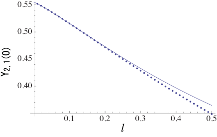
(a)

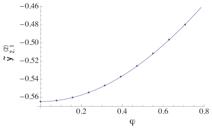
(b)

Figure 3: (a) Plots of $Y_{2,1}(0)$ from numerics (points) and from the analytic expansion (solid line) for $m_{1}=m_{2}=l$.   (b) Phase dependence of an expansion coefficient of $\tilde{Y}_{2,1}(0)$. The points are from numerical fitting, whereas the solid line represents the analytic expression.

6 UV expansion of remainder function

Based on the results so far, we derive the UV expansion of the remainder function in this section.

6.1 Remainder function for six-cusp minimal surfaces

In the case of $n=6$ ($N=2$), the relevant cross-ratios for $\Delta A_{\rm BDS}$ in (2.32) are

$$u_{r,r+3}=\bigl{(}U_{1}^{[2r-1]}\bigr{)}^{-1}=\frac{1}{T_{2,1}^{[2r-2]}T_{2,1}^{[2r]}}\,.$$ (6.1)

These are also rewritten by using $T_{2,1}^{[6+r]}=T_{2,1}^{[r]}$. In the UV limit, the cross-ratios become $u_{r,r+3}=1/4$ and equal to each other. Form (6.1) and the expansion of the T-functions, one finds that $\Delta A_{\rm BDS}$ is expanded in terms of $t_{a,s}^{(0,0)}$, $(t_{a,s}^{(2,0)})^{2}$ and $t_{a,s}^{(0,4)}$ for real $m_{s}$ up to ${\cal O}(l^{4(1-\Delta)})$. Similarly to the AdS₃ case [26, 27], other $t_{a,s}^{(p,2q)}$ do not appear in the expansion due to the ${\mathbb{Z}}_{n}$-symmetry. Further using (5.32) and (5.35), we find

$$\Delta A_{\rm BDS}=\frac{3}{4}\operatorname{Li_{2}}(-3)-\frac{1}{16}(3+2\log 2)(t_{2,1}^{(2,0)})^{2}l^{4(1-\Delta)}+{\mathcal{O}}(l^{6(1-\Delta)})\,.$$ (6.2)

Since the period term and the bulk term in the free energy part cancel each other, we arrive at the expansion of the remainder function,

$$R_{6}=\frac{\pi}{6}+\frac{3}{4}\operatorname{Li_{2}}(-3)+\Bigl{[}\frac{\pi}{6}C_{6}^{(2)}-\frac{1}{16}(3+2\log 2)(\tilde{t}_{1,1}^{(2,0)})^{2}\Bigr{]}(\kappa_{6}G)^{2}\cdot l^{8/3}+{\mathcal{O}}(l^{4})\,,$$ (6.3)

where we have introduced

$$\tilde{t}_{a,s}^{(2,0)}:={t}_{a,s}^{(2,0)}/\kappa_{n}G\,,$$ (6.4)

and $C_{6}^{(2)}$, $t_{1,1}^{(2,0)}$ and $\kappa_{6}G$ are given by (4.7), (5.32) and (4.8) with $G=\tilde{M}_{1}=1$, respectively. For complex $m_{s}$, one has only to replace $G^{2}(\tilde{M}_{s})$ by $|G(\tilde{M}_{s}e^{i\varphi_{s}})|^{2}$, giving just $|G|^{2}=1$. These results agree with those in [22].

6.2 Remainder function for seven-cusp minimal surfaces

In the case of $n=7$ ($N=3$), the relevant cross-ratios for $\Delta A_{\rm BDS}$ in (2.33) are

$$u_{r,r+3}=\bigl{(}U_{2}^{[2r-2]}\bigr{)}^{-1}=\frac{T_{2,1}^{[2r-2]}}{T_{2,2}^{[2r-3]}T_{2,2}^{[2r-1]}}\,.$$ (6.5)

These are also rewritten by using $T_{2,1}^{[7+r]}=T_{2,2}^{[r]}$. From (6.5) and the expansion of the T-functions, one finds again that $\Delta A_{\rm BDS}$ is expanded in terms of $t_{a,s}^{(0,0)}$, $(t_{a,s}^{(2,0)})^{2}$ and $t_{a,s}^{(0,4)}$ for real $m_{s}$ up to ${\cal O}(l^{4(1-\Delta)})$. Further using (5.38) and (5.39), we find that

$$\Delta A_{\rm BDS}=D_{7}^{(0)}+D_{7}^{(4)}(t_{1,1}^{(2,0)})^{2}l^{4(1-\Delta)}+{\mathcal{O}}(l^{6(1-\Delta)})\,,$$ (6.6)

where

$$D_{7}^{(0)} = -\frac{7}{4}\left[\log^{2}\left(2\cos\frac{\pi}{7}+1\right)+\operatorname{Li}_{2}\left(\frac{2\cos\frac{\pi}{7}}{2\cos\frac{\pi}{7}+1}\right)\right]\,,$$ (6.7)

$$D_{7}^{(4)} = -\frac{7}{16s_{0}(15+5s_{0}-24s_{0}^{2})}\bigl{[}s_{0}(3-4s_{0})+(1-s_{0})(1-4s_{0})\log(3-4s_{0}^{2})\bigr{]}\,.$$

Due to the cancelation between the period and bulk terms, we arrive at the expansion of the remainder function,

$$R_{7}=\frac{\pi}{6}c_{7}+D_{7}^{(0)}+\Bigl{[}\frac{\pi}{6}C_{7}^{(2)}+D_{7}^{(4)}(\tilde{t}_{1,1}^{(2,0)})^{2}\Bigr{]}(\kappa_{7}G)^{2}\cdot l^{16/7}+{\mathcal{O}}(l^{24/7})\,,$$ (6.8)

where $C_{7}^{(2)}$, $t_{1,1}^{(2,0)}$ and $\kappa_{7}G(\tilde{M}_{s})$ are given by (4.7), (5.38) and (4.25), respectively. For complex $m_{s}$, $\bigl{(}\kappa_{7}G(\tilde{M}_{s})\bigr{)}^{2}$ is replaced by $|\kappa_{7}G(\tilde{M}_{s}e^{i\varphi_{s}})|^{2}$.

In Fig. 4, we show plots of the 7-point (7-cusp) remainder function for $m_{1}=e^{-\frac{\pi}{40}i}l$, $m_{2}=e^{-\frac{\pi}{20}i}l$ from numerics (points) and from our analytic expansion (solid line). They are in good agreement around the UV limit.

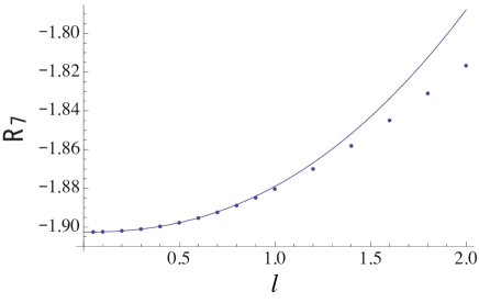
Figure 4: 7-point remainder function at strong coupling. The points are from numerics, whereas the solid line is from our analytic expansion (6.8). These are evaluated for $m_{1}=e^{-\frac{\pi}{40}i}l$, $m_{2}=e^{-\frac{\pi}{20}i}l$.

6.3 Rescaled remainder function

In [29], it was observed numerically for the 8-cusp minimal surfaces in AdS₃ that the remainder functions at strong coupling and at two loops are close to each other, but different, if they are appropriately shifted and rescaled. In [26, 27], this was analytically demonstrated around the UV limit for the general null-polygonal minimal surfaces in AdS₃.

Similarly, one can define the rescaled remainder function for the AdS₄ case by

$$\bar{R}_{n}:=\frac{R_{n}-R_{n,{\rm UV}}}{R_{n,{\rm UV}}-R_{n,{\rm IR}}}\,.$$ (6.9)

Here, $R_{n,{\rm UV}}$ is the $n$-point remainder function in the UV limit, which is read off from (6.3) and (6.8). $R_{n,{\rm IR}}$ is the $n$-point remainder function in the IR limit where $|m_{s}|\to\infty$. To find this constant, we note the asymptotics of $Y_{a,s}$ (2.1) valid for real $m_{s}$ and $|\operatorname{Im}\theta\,|<\pi/2$, and successively use the Y-system (2.5), to express $Y_{a,s}^{[r]}$, e.g., by $Y_{a,s}^{[0]}$ and $Y_{a,s}^{[-1]}$ in the IR limit. We then find that

$$(u_{1,4},u_{2,5},u_{3,6})\sim(e^{-m_{1}},1,e^{-m_{1}})\,,$$ (6.10)

for $n=6$ [13], and that

$$(u_{1,4},u_{2,5},u_{3,6},u_{4,7},u_{1,5},u_{2,6},u_{3,7})\sim\Bigl{(}e^{-\sqrt{2}m_{2}},\frac{1}{2},1,e^{-m_{1}},e^{-m_{1}},1,\frac{1}{2}\Bigr{)}\,,$$ (6.11)

for $n=7$. The leading terms in $\Delta A_{\rm BDS}$ thus cancel $A_{\rm periods}$ [23]. Furthermore, from the fact that $A_{\rm free}$ vanishes in the IR limit, it follows that

$$R_{6,{\rm IR}}=-\frac{\pi^{2}}{12}\,,\qquad R_{7,{\rm IR}}=-\frac{\pi^{2}}{6}\,.$$ (6.12)

Substituting these values into (6.9), we find that

$$\bar{R}_{6}\approx-0.0528126l^{8/3}+{\cal O}(l^{12/3})\,,$$ (6.13)

for $n=6$, and

$$\bar{R}_{7}\approx-0.707647|\kappa_{7}G|^{2}l^{16/7}+{\cal O}(l^{24/7})\,,$$ (6.14)

for $n=7$.

On the weak-coupling side, the remainder function at two loops for $n=6$ in the AdS₄ case is read off from the results in the AdS₅ case [32, 33, 34, 35]. In particular, one can find the UV expansion of the remainder function from a very concise expression in [35] and the expansion of the T-functions in the previous section: $R_{6}^{\rm 2\mbox{-}loop}\approx 1.08917-0.0487985l^{8/3}$. The value in the UV limit $l\to 0$ has been given in [32, 34]. The rescaled remainder function is defined similarly to (6.9). Since the two-loop remainder function vanishes in the IR limit, the rescaled remainder function at two loops is expanded as

$$\bar{R}_{6}^{\rm 2\mbox{-}loop}\approx-0.0448036l^{8/3}+{\cal O}(l^{12/3})\,.$$ (6.15)

The ratio of the rescaled remainder functions at strong coupling and at two loops is then

$${\bar{R}_{6}\over\bar{R}_{6}^{\rm 2\mbox{-}loop}}\approx 1.17876\,,$$ (6.16)

which is close to 1. By numerics, we also find that the two 6-point rescaled remainder functions are close to each other for all the scales as shown in Fig. 5 (a). We also show the 7-point rescaled remainder function from the numerics in Fig. 5 (b). For both the 6- and 7-point cases, we find a good agreement with our analytic expansions around the UV limit. It would be of interest to compare the 7-point rescaled remainder function at strong coupling with the one at weak coupling, which is yet to be computed.

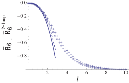
(a)

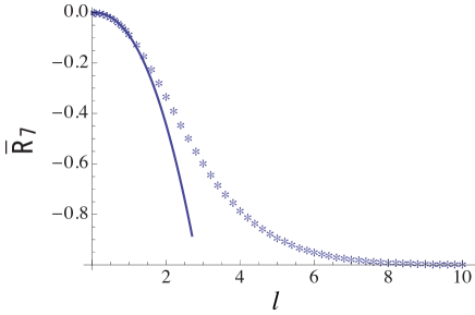
(b)

Figure 5: (a) 6-point rescaled remainder functions. Points denoted by $\ast$/$+$ stand for a plot from numerics at strong coupling/two loops. The solid/dashed line represents the analytic expansion around the UV limit at strong coupling/two loops. These are evaluated for $m_{1}=e^{-\frac{\pi}{20}i}l$.   (b) 7-point rescaled remainder function at strong coupling. Points are from numerics and the solid line represents the analytic expansion around the UV limit. These are evaluated for $m_{1}=e^{-\frac{\pi}{40}i}l$, $m_{2}=e^{-\frac{\pi}{20}i}l$.

6.4 Cross-ratios and mass parameters

We have expanded the remainder function by the mass parameters. In order to express it by the cross-ratios, one needs to invert the relation between the former and the latter.

For $n=6$, it follows from (6.1) and the expansion of the T-functions in the previous section that

$$u_{r,3+r}=\frac{1}{4}-\frac{1}{8}\cos\Bigl{(}\frac{1}{3}(4\varphi-(2r-1)\pi)\Bigr{)}\cdot|t_{2}^{(2,0)}|l^{2(1-\Delta)}+{\mathcal{O}}(l^{4(1-\Delta)})\,.$$ (6.17)

Inverting this relation, one can express the mass parameter $m_{1}=e^{i\varphi}l$ by the cross-ratios [22]. In the notation in this paper, the result reads as

$$\tan\frac{4}{3}\varphi = \frac{\sqrt{3}(U_{1}^{[-1]}-U_{1}^{[1]})}{2U_{1}^{[3]}-U_{1}^{[-1]}-U_{1}^{[1]}}\,,\qquad l^{\frac{4}{3}}=\frac{-2U_{1}^{[3]}+U_{1}^{[-1]}+U_{1}^{[1]}}{6\sqrt{3}|t_{1}^{(2,0)}|\cos\frac{4}{3}\varphi}\,.$$ (6.18)

For $n=7$, it follows from (6.5) and the expansion of the T-function in the previous section that

$$u_{r,r+3}=\frac{1}{t_{2,1}^{(0,0)}}-\frac{2\cos\frac{2\pi}{7}-1}{2(t_{2,1}^{(0,0)})^{2}}\Bigl{(}t_{2,1}^{(2,0)}e^{-\frac{4}{7}\pi(r-1)i}+\bar{t}_{2,1}^{(2,0)}e^{\frac{4}{7}\pi(r-1)i}\Bigr{)}l^{2(1-\Delta)}+{\mathcal{O}}(l^{3(1-\Delta)})\,.$$ (6.19)

By inverting this relation, one can express the mass parameters by the cross-ratios. For example, when $\varphi_{1}=\varphi_{2}$, the inversion is simple, but generically it is not.

7 Conclusions and discussion

In this paper we have evaluated the regularized area of the null-polygonal minimal surfaces in AdS₄, and the remainder function for the corresponding Wilson loops/amplitudes at strong coupling. They are described by the TBA integral equations or the associated T-/Y-system of the HSG model, which is regarded as the integrable perturbation of the generalized parafermion CFT by the weight-zero adjoint fields. The connection to the HSG model as well as to the corresponding CFT allows us to derive the analytic expansion of the remainder function around the UV/regular-polygonal limit by using the conformal perturbation theory. Generalizing the results in the AdS₃ case, we have found or argued that the TBA systems in the single-mass cases are given by those for the perturbed $\mathrm{SU}(4)$ diagonal coset models and $W$ minimal models. This is used to find the precise expansion coefficients through their mass-coupling relations and correlation functions. We have derived the leading-order expansion explicitly for $n=6$ and 7. For the 6-point case, we have also compared the rescaled remainder function with the two-loop one. They are close to each other, but different, similarly to the AdS₃ case. Although we have focused on the $n\notin 4{\mathbb{Z}}$ case in this paper, it would be an interesting problem to generalize our analysis to the minimal surfaces with general $n$, and to compare their remainder functions with those at weak coupling.

As noted in section 4, the TBA equations for the AdS₄ minimal surfaces generally exhibit a numerical instability around the UV limit. In spite of that, our analytic expansion works well, which proves our formalism to be useful in this respect as well. It would also be desirable to establish the proposed connection to the TBA systems of the non-unitary diagonal coset/$W$ minimal models, and to substantiate the “decomposition” discussed in section 3.

The remainder function at strong coupling for general kinematical configurations are given by the minimal surfaces in AdS₅. The corresponding TBA system is recovered by reintroducing the parameters dropped in the AdS₄ case. For example, in the 6-point case, the relevant chemical potential is turned on by a twist operator in the ${\mathbb{Z}}_{4}$-parafermion or the $\mathrm{SU}(2)_{4}/\mathrm{U}(1)$ coset CFT. It would be interesting to find corresponding operators for higher-point cases, as well as to identify the relevant integrable system and the CFT. This would also provide a way to analyze the AdS₄ minimal surfaces with the chemical potential $\mu=-1$, which are not discussed in this paper. Finally, it would be very interesting to find the quantum/strong-coupling corrections to the minimal surfaces, and possibly to extrapolate the results to the weak-coupling side.

Acknowledgements

We would like to thank Y. Aisaka, Z. Bajnok, J. Balog, P. Dorey, C. Dunning, D. Fioravanti, K. Hosomichi, J.L. Miramontes, M. Rossi, K. Sakai, V. Schomerus, J. Suzuki and R. Tateo for useful discussions and conversations. We are also grateful to Yukawa Institute for Theoretical Physics, where part of this work was done during YITP workshop YITP-W-12-05. Y. S. would like to thank the organizers of a conference “Progress in Quantum Field Theory and String Theory” at Osaka, CQUeST-IEU Focus program at Seoul, APCTP-CQueST-IEU Workshop at Jeju Island, Yukawa International Seminar (YKIS) 2012 at Kyoto, and YIPQS long-term workshop at Kyoto, for warm hospitality. The work of Y. H. is supported in part by the JSPS Research Fellowship for Young Scientists, whereas the work of K. I. and Y. S. is supported in part by Grant-in-Aid for Scientific Research from the Japan Ministry of Education, Culture, Sports, Science and Technology.

A Three-point function in $W$ minimal models

In this appendix we review the free field representation of the $WA_{k-1}^{(p,q)}$ minimal model and compute the three-point function of the ground-state and perturbing operators for $k=4$ and $p=5,q=7$, that is used in section 4 to analyze the 7-point remainder function. To lighten the notation, we refrain from using boldface letters for the weight vectors.

A.1 Free field representation

The $WA_{k-1}$ minimal model [48] is realized by the scalar fields $\varphi=(\varphi_{1},...,\varphi_{k-1})$ in the $\mathfrak{sl}(k)$ conformal Toda field theory with the Lagrangian,

$$L=\frac{1}{8\pi}(\partial\varphi)^{2}+\tilde{\mu}\sum_{j=1}^{k-1}e^{b(e_{j},\varphi)}\,.$$ (A.1)

Here, $e_{j}$ are the simple roots of $\mathfrak{sl}(k)$, $(\ ,\ )$ denotes the inner-product, $\tilde{\mu}$ is the scale parameter and $b$ is the dimensionless coupling. The system has the background charge,

$$Q=\Bigl{(}b+\frac{1}{b}\Bigr{)}\rho\,,$$ (A.2)

where $\rho=\sum_{j}\omega_{j}$ is the Weyl vector of $\mathfrak{sl}(k)$ and $\omega_{j}$ are the fundamental weights satisfying $(e_{i},\omega_{j})=\delta_{ij}$. The energy momentum tensor is

$$T(z)=-\frac{1}{2}(\partial\varphi)^{2}+(Q,\partial^{2}\varphi)\,.$$ (A.3)

The central charge is given by

$$c=k-1+12Q^{2}=(k-1)\Bigl{[}1+k(k+1)\Bigl{(}b+\frac{1}{b}\Bigr{)}^{2}\Bigr{]}\,.$$ (A.4)

For the $WA_{k-1}^{(p,q)}$ minimal model with the central charge (3.5), the coupling is given by

$$ib=\sqrt{\frac{p}{q}}.$$ (A.5)

The primary field of the CFT is represented by the vertex operator,

$$V_{\alpha}:=e^{(\alpha,\varphi)}\,,$$ (A.6)

which has the dimension

$$h(\alpha)=h(2Q-\alpha)=\frac{1}{2}(\alpha,2Q-\alpha)\,.$$ (A.7)

Thus, the field with the dimension (3.14) is represented by the vertex operator with

$$\alpha=\alpha(\Lambda_{+},\Lambda_{-}):=-\frac{1}{b}\Lambda_{+}-b\Lambda_{-}\,.$$ (A.8)

For example, from (3.17), we find that the operator $\phi_{(1,1,{\rm ad})}$ corresponds to $V_{\alpha}$ with

$$\alpha=\alpha_{(1,1,{\rm adj})}:=-be_{0}\,,$$ (A.9)

where

$$e_{0}=\sum_{j=1}^{k-1}e_{j}=\omega_{1}+\omega_{k-1}$$ (A.10)

is the highest root, i.e., the highest weight of the adjoint representation. Similarly, from (3.19), the ground-state operator for $k=4$ and $p=n-2,q=n$ with $n$ odd corresponds to

$$\alpha=\alpha_{0}:=-\Bigl{(}\frac{n-7}{2}b^{-1}+\frac{n-5}{2}b\Bigr{)}\omega_{2}\,.$$ (A.11)

For $n=7$, this simplifies to

$$\alpha_{0}=-b\omega_{2}.$$ (A.12)

A.2 Three-point function

We are interested in the three-point structure constant $C_{\phi_{0}\phi_{(1,1,{\rm adj})}\phi_{0}}$ of the ground-state operator $\phi_{0}$ and the perturbing operator $\phi_{(1,1,{\rm adj})}$ for $k=4$ and $p=5,q=7$, where

$$\phi_{0}\sim V_{\alpha_{0}}\,,\quad\phi_{(1,1,{\rm adj})}\sim V_{-be_{0}}\,,$$ (A.1)

up to normalization. To compute this, we first note that the normalized three-point function is generally given by [71, 72]

$$\big{\langle}{\cal O}_{\alpha_{1}}{\cal O}_{\alpha_{2}}{\cal O}_{\alpha_{3}}\big{\rangle}_{\rm normalized}=B(\alpha_{1})B(\alpha_{2})B^{-1}(\alpha_{3})\big{\langle}V_{\alpha_{1}}V_{\alpha_{2}}V_{2Q-\alpha^{\ast}_{3}}\big{\rangle}\,,$$ (A.2)

where ${\cal O}_{\alpha}:=B(\alpha)V_{\alpha}$ is the normalized operator so that $\bigl{\langle}{\cal O}_{\alpha}(z){\cal O}_{\alpha^{\ast}}(0)\bigr{\rangle}_{\rm normalized}=|z|^{-4h(\alpha)}$, and $\alpha^{\ast}$ for $\alpha$ is defined through $(\alpha,e_{j})=(\alpha^{\ast},e_{k-j})$. The normalization constant $B(\alpha)$ is given by

$$B(\alpha) = \sqrt{A(\alpha)A(2Q)\over A(2Q-\alpha)A(0)}\,,$$

$$A(\alpha) = \Bigl{(}\pi\tilde{\mu}\gamma(b^{2})\Bigr{)}^{(\alpha-Q,\rho)/b}\prod_{e>0}\Gamma\bigl{(}1-b(\alpha-Q,e)\bigr{)}\Gamma\bigl{(}-b^{-1}(\alpha-Q,e)\bigr{)}\,,$$ (A.3)

with the product being over the positive roots. The normalization of the vacuum has also been taken into account. Next, the unnormalized structure constant $C^{\alpha_{3}}_{\alpha_{1},\alpha_{2}}$ is obtained by extracting the residue of the Coulomb-gas integral for $\bigl{\langle}V_{\alpha_{1}}(\infty)V_{\alpha_{2}}(1)V_{2Q-\alpha_{3}}(0)\bigr{\rangle}$. In particular, a class of the structure constants has been evaluated in eq. (1.53) of [71]:

$$C^{\alpha}_{-be_{0},\alpha} = \sum_{i=1}^{k}\prod_{j\neq i}^{k}{\pi\tilde{\mu}\gamma\bigl{(}b(\alpha-Q,h_{ji})\bigr{)}\over\gamma(-b^{2})\gamma\bigl{(}1+b^{2}+b(\alpha-Q,h_{ji})\bigr{)}}{\cal F}_{i}^{2}(\alpha)\,,$$ (A.4)

where

$${\cal F}_{i}(\alpha) := 1+\sum_{p=1}^{\infty}\prod_{j=1}^{k}{\bigl{(}b(Q-\alpha,h_{ji})-b^{2}\bigr{)}_{p}\over\bigl{(}1+b(Q-\alpha,h_{ji})\bigr{)}_{p}}$$ (A.7)

$$= {}_{k}F_{k-1}\left(\begin{array}[]{ccccc}b(Q-\alpha,h_{1i})-b^{2},&\cdots,&-b^{2},&\cdots,&b(Q-\alpha,h_{ki})-b^{2}\\ 1+b(Q-\alpha,h_{1i}),&\cdots&&\cdots,&1+b(Q-\alpha,h_{ki})\end{array}\bigg{|}\ 1\,\right)\,,\quad$$

and the $i$-th entry in the lower row is empty. We have also defined

$$(x)_{p}=x(x+1)\cdots(x+p-1)={\Gamma(x+p)\over\Gamma(x)}\,,$$ (A.8)

$\gamma(x)=\Gamma(x)/\Gamma(1-x)$ and

$$h_{ij}:=h_{i}-h_{j}\,,\qquad h_{j}=\omega_{1}-e_{1}-\cdots-e_{j-1}\,.$$ (A.9)

We now concentrate on the case of $k=4$. Since $\alpha_{0}=-b\omega_{2}$ for $p=5,q=7$ of our interest, we first evaluate $C^{-b\omega_{2}}_{-be_{0},-b\omega_{2}}$ with $b$ being generic. Taking into account the fact that the coefficients in front of ${\cal F}_{i}$ in (A.4) vanish for $i=2,4$, we find after some algebras that

$$C^{-b\omega_{2}}_{-be_{0},-b\omega_{2}} = \Bigl{(}{\pi\tilde{\mu}\over\gamma(-b^{2})}\Bigr{)}^{3}{\gamma(1+b^{2})\over\gamma(2+2b^{2})}\Bigl{[}{\gamma(2+3b^{2})\over\gamma(4+5b^{2})}{\cal F}_{1}^{2}(-b\omega_{2})+{\gamma(-2-3b^{2})\over\gamma(-b^{2})}{\cal F}_{3}^{2}(-b\omega_{2})\Bigr{]}\,,$$ (A.10)

$$= \Bigl{(}{\pi\tilde{\mu}\over\gamma(-b^{2})}\Bigr{)}^{3}{\gamma^{2}(1+b^{2})\over\gamma(2+2b^{2})\gamma(4+5b^{2})}{\Gamma^{2}(3+4b^{2})\over\Gamma^{2}(2+2b^{2})}\cdot(-2)\cos(2\pi b^{2})\,,$$

where

$${\cal F}_{1}(-b\omega_{2}) = {}_{4}F_{3}\biggl{(}\begin{array}[]{cccc}-b^{2},&-1-2b^{2},&-2-4b^{2},&-3-5b^{2}\\ &-b^{2},&-1-3b^{2},&-2-4b^{2}\end{array}\bigg{|}\ 1\,\biggr{)}$$

$$= {\Gamma(-1-3b^{2})\Gamma(3+4b^{2})\over\Gamma(-b^{2})\Gamma(2+2b^{2})}\,,$$

$${\cal F}_{3}(-b\omega_{2}) = {}_{4}F_{3}\biggl{(}\begin{array}[]{cccc}-b^{2},&2+2b^{2},&1+b^{2},&-1-2b^{2}\\ &3+3b^{2},&2+2b^{2},&-b^{2}\end{array}\bigg{|}\ 1\,\biggr{)}$$

$$= {\Gamma(3+3b^{2})\Gamma(3+4b^{2})\over\Gamma(2+2b^{2})\Gamma(4+5b^{2})}\,.$$

To obtain the normalized structure constant through (A.2), we next need $B(-be_{0})$, which is evaluated by using

$${A(\alpha)\over A(2Q-\alpha)} = \Bigl{(}\pi\tilde{\mu}\gamma(b^{2})\Bigr{)}^{2(\alpha-Q,\rho)/b}\prod_{e>0}\frac{1}{b^{2}}{\gamma\bigl{(}1-b(\alpha-Q,e)\bigr{)}\over\gamma\bigl{(}1+b^{-1}(\alpha-Q,e)\bigr{)}}\,,$$ (A.17)

as

$$B^{2}(-be_{0})=\Bigl{(}\pi\tilde{\mu}\gamma(b^{2})\Bigr{)}^{-6}b^{-24}\Bigl{(}{3+4b^{2}\over 4+5b^{2}}\Bigr{)}^{2}\gamma^{-2}(1+b^{2})\gamma(3+3b^{2})\gamma(5+5b^{2})\,.$$ (A.18)

Combining (A.10) and (A.18), we find the normalized structure constant,

$$C^{-b\omega_{2};\ {\rm normalized}}_{-be_{0},-b\omega_{2}} = B(-be_{0})C^{-b\omega_{2}}_{-be_{0},-b\omega_{2}}$$

$$= -2\cos(2\pi b^{2})\cdot(3+4b^{2})(4+5b^{2}){\Gamma^{2}(3+4b^{2})\over\Gamma^{2}(2+2b^{2})}{\gamma(1+b^{2})\over\gamma(2+2b^{2})}\sqrt{\gamma(3+3b^{2})\over\gamma(5+5b^{2})}\,.$$

The factors of $\pi\tilde{\mu}$ have been canceled, as they should.

Finally, the normalized structure constant $C_{\phi_{0}\phi_{(1,1,{\rm adj})}\phi_{0}}$ for $p=5,q=7$ and $k=4$ is obtained by plugging $b^{2}=-5/7$ in the above expression,

$$C_{\phi_{0}\phi_{(1,1,{\rm adj})}\phi_{0}}=-\frac{6}{49}\cos\Bigl{(}\frac{10}{7}\pi\Bigr{)}{\Gamma^{2}(\frac{1}{7})\gamma(\frac{2}{7})\over\Gamma^{2}(\frac{4}{7})\gamma(\frac{4}{7})}\sqrt{\gamma(\frac{6}{7})\over\gamma(\frac{10}{7})}\approx 1.31083\sqrt{-1}\,.$$ (A.20)

This is purely imaginary since $\gamma(10/7)<0$. In subsection 4.2, $\phi_{0}$ and $\phi_{(1,1,{\rm adj})}$ for $WA_{3}^{(5,7)}$ are denoted by $\hat{\Phi}_{0}$ and $\hat{\Phi}$, respectively.

References

References

- [1] S. -J. Rey and J. -T. Yee, Eur. Phys. J. C 22 (2001) 379 [hep-th/9803001].
- [2] J. M. Maldacena, Phys. Rev. Lett. 80 (1998) 4859 [hep-th/9803002].
- [3] L. F. Alday and J. M. Maldacena, JHEP 0706 (2007) 064 [arXiv:0705.0303 [hep-th]].
- [4] J.M. Drummond, G.P. Korchemsky and E. Sokatchev, Nucl. Phys. B 795 (2008) 385 [arXiv:0707.0243 [hep-th]].
- [5] A. Brandhuber, P. Heslop and G. Travaglini, Nucl. Phys. B 794 (2008) 231 [arXiv:0707.1153 [hep-th]].
- [6] J. M. Drummond, J. Henn, V. A. Smirnov and E. Sokatchev, JHEP 0701 (2007) 064 [arXiv:hep-th/0607160].
- [7] J.M. Drummond, J. Henn, G.P. Korchemsky and E. Sokatchev, Nucl. Phys. B 826 (2010) 337 [arXiv:0712.1223 [hep-th]].
- [8] Z. Bern, L. J. Dixon and V. A. Smirnov, Phys. Rev. D 72 (2005) 085001 [arXiv:hep-th/0505205].
- [9] L. F. Alday and J. Maldacena, JHEP 0711 (2007) 068 [arXiv:0710.1060 [hep-th]].
- [10] Z. Bern, L. J. Dixon, D. A. Kosower, R. Roiban, M. Spradlin, C. Vergu and A. Volovich, Phys. Rev. D 78 (2008) 045007 [arXiv:0803.1465 [hep-th]].
- [11] J. M. Drummond, J. Henn, G. P. Korchemsky and E. Sokatchev, Nucl. Phys. B 815 (2009) 142 [arXiv:0803.1466 [hep-th]].
- [12] L. F. Alday and J. Maldacena, JHEP 0911 (2009) 082 [arXiv:0904.0663 [hep-th]].
- [13] L. F. Alday, D. Gaiotto and J. Maldacena, JHEP 1109 (2011) 032 [arXiv:0911.4708 [hep-th]].
- [14] L. F. Alday, J. Maldacena, A. Sever and P. Vieira, J. Phys. A 43 (2010) 485401 [arXiv:1002.2459 [hep-th]].
- [15] Y. Hatsuda, K. Ito, K. Sakai and Y. Satoh, JHEP 1004 (2010) 108 [arXiv:1002.2941 [hep-th]].
- [16] C. R. Fernandez-Pousa, M. V. Gallas, T. J. Hollowood, J. L. Miramontes, Nucl. Phys. B 484 (1997) 609 [arXiv:hep-th/9606032].
- [17] Al. B. Zamolodchikov, Nucl. Phys. B 342 (1990) 695.
- [18] P. Dorey, I. Runkel, R. Tateo and G. Watts, Nucl. Phys. B 578 (2000) 85 [arXiv:hep-th/9909216].
- [19] P. Dorey, A. Lishman, C. Rim and R. Tateo, Nucl. Phys. B 744 (2006) 239 [arXiv:hep-th/0512337].
- [20] I. Affleck, A. W. W. Ludwig, Phys. Rev. Lett. 67 (1991) 161.
- [21] G. Yang, JHEP 1012, 082 (2010) [arXiv:1004.3983 [hep-th]].
- [22] Y. Hatsuda, K. Ito, K. Sakai and Y. Satoh, JHEP 1009 (2010) 064 [arXiv:1005.4487 [hep-th]].
- [23] G. Yang, JHEP 1103 (2011) 087 [arXiv:1006.3306 [hep-th]].
- [24] J. Bartels, J. Kotanski and V. Schomerus, JHEP 1101 (2011) 096 [arXiv:1009.3938 [hep-th]].
- [25] J. Bartels, V. Schomerus and M. Sprenger, arXiv:1207.4204 [hep-th].
- [26] Y. Hatsuda, K. Ito, K. Sakai and Y. Satoh, JHEP 1104 (2011) 100 [arXiv:1102.2477 [hep-th]].
- [27] Y. Hatsuda, K. Ito and Y. Satoh, JHEP 1202 (2012) 003 [arXiv:1109.5564 [hep-th]].
- [28] D. Gepner, Nucl. Phys. B 290 (1987) 10.
- [29] A. Brandhuber, P. Heslop, V. V. Khoze and G. Travaglini, JHEP 1001 (2010) 050 [arXiv:0910.4898 [hep-th]].
- [30] V. Del Duca, C. Duhr and V. A. Smirnov, JHEP 1009 (2010) 015 [arXiv:1006.4127 [hep-th]].
- [31] P. Heslop and V. V. Khoze, JHEP 1011 (2010) 035 [arXiv:1007.1805 [hep-th]].
- [32] C. Anastasiou, A. Brandhuber, P. Heslop, V. V. Khoze, B. Spence and G. Travaglini, JHEP 0905 (2009) 115 [arXiv:0902.2245 [hep-th]].
- [33] V. Del Duca, C. Duhr and V. A. Smirnov, JHEP 1003 (2010) 099 [arXiv:0911.5332 [hep-ph]].
- [34] V. Del Duca, C. Duhr and V. A. Smirnov, JHEP 1005 (2010) 084 [arXiv:1003.1702 [hep-th]].
- [35] A. B. Goncharov, M. Spradlin, C. Vergu and A. Volovich, Phys. Rev. Lett. 105 (2010) 151605 [arXiv:1006.5703 [hep-th]].
- [36] O. A. Castro-Alvaredo, A. Fring, C. Korff and J. L. Miramontes, Nucl. Phys. B 575 (2000) 535 [arXiv:hep-th/9912196].
- [37] J. L. Miramontes and C. R. Fernandez-Pousa, Phys. Lett. B 472 (2000) 392 [arXiv:hep-th/9910218].
- [38] R. Koberle and J. A. Swieca, Phys. Lett. B 86 (1979) 209.
- [39] H. W. Braden, E. Corrigan, P. E. Dorey and R. Sasaki, Nucl. Phys. B 338 (1990) 689.
- [40] G. Mussardo, “Statistical field theory:an introduction to exactly solved models in statistical physics,” Oxford Univ. Press, Oxford, UK (2009).
- [41] Al. B. Zamolodchikov, Nucl. Phys. B 366 (1991) 122.
- [42] H. Itoyama, P. Moxhay, Phys. Rev. Lett. 65 (1990) 2102.
- [43] Al. B. Zamolodchikov, Nucl. Phys. B 358 (1991) 497.
- [44] F. Ravanini, R. Tateo and A. Valleriani, Int. J. Mod. Phys. A 8 (1993) 1707 [hep-th/9207040].
- [45] P. Fendley, JHEP 0105, 050 (2001) [arXiv:hep-th/0101034].
- [46] F. Ravanini, Phys. Lett. B 282, 73 (1992) [hep-th/9202020].
- [47] F. Ravanini, R. Tateo and A. Valleriani, Phys. Lett. B 293 (1992) 361 [hep-th/9207069].
- [48] V. A. Fateev and S. L. Lukyanov, Int. J. Mod. Phys. A 3 (1988) 507.
- [49] V. G. Kac and M. Wakimoto, Acta. Appl. Math. 21 (1990) 3.
- [50] E. Frenkel, V. Kac and M. Wakimoto, Commun. Math. Phys. 147 (1992) 295.
- [51] P. Mathieu, D. Senechal and M. Walton, Int. J. Mod. Phys. A 7S1B (1992) 731 [hep-th/9110003].
- [52] D. Altschuler, Nucl. Phys. B 313 (1989) 293.
- [53] A. Kuniba, T. Nakanishi and J. Suzuki, Nucl. Phys. B 356 (1991) 750.
- [54] V. A. Fateev and A. B. Zamolodchikov, Sov. Phys. JETP 62 (1985) 215 [Zh. Eksp. Teor. Fiz. 89 (1985) 380].
- [55] D. Gepner and Z. -a. Qiu, Nucl. Phys. B 285 (1987) 423.
- [56] F. A. Bais, P. Bouwknegt, M. Surridge and K. Schoutens, Nucl. Phys. B 304 (1988) 371.
- [57] J. Bagger and D. Nemeschansky, “Coset construction of chiral algebras,” HUTP-88/A059.
- [58] P. Bouwknegt and K. Schoutens, Phys. Rept. 223 (1993) 183 [hep-th/9210010].
- [59] M. Ninomiya and K. Yamagishi, Phys. Lett. B 183 (1987) 323 [Addendum-ibid. B 190 (1987) 234].
- [60] V.G. Kac and M. Wakimoto, Adv. Math. 70 (1988) 156.
- [61] V. A. Fateev, Phys. Lett. B 324 (1994) 45.
- [62] C. Dunning, Phys. Lett. B 537 (2002) 297 [hep-th/0204090].
- [63] T. R. Klassen and E. Melzer, Nucl. Phys. B 350, 635 (1991).
- [64] O. Castro-Alvaredo and A. Fring, Phys. Lett. A 334 (2005) 173 [hep-th/0406066].
- [65] V. V. Bazhanov, S. L. Lukyanov and A. B. Zamolodchikov, Commun. Math. Phys. 177 (1996) 381 [arXiv:hep-th/9412229].
- [66] A. Fring and R. Koberle, Nucl. Phys. B 421 (1994) 159 [arXiv:hep-th/9304141].
- [67] S. Ghoshal and A. B. Zamolodchikov, Int. J. Mod. Phys. A 9 (1994) 3841 [Erratum-ibid. A 9 (1994) 4353] [arXiv:hep-th/9306002].
- [68] R. Sasaki, “Reflection Bootstrap equations for Toda field theory,” in the proceedings of the conference, Interface between physics and mathematics, eds. W. Nahm and J.-M. Shen [arXiv:hep-th/9311027].
- [69] P. Dorey, D. Fioravanti, C. Rim and R. Tateo, Nucl. Phys. B 696 (2004) 445 [arXiv:hep-th/0404014].
- [70] T. Gannon, arXiv:hep-th/0106123.
- [71] V. A. Fateev and A. V. Litvinov, JHEP 0711 (2007) 002 [arXiv:0709.3806 [hep-th]].
- [72] C. -M. Chang and X. Yin, JHEP 1210 (2012) 050 [arXiv:1112.5459 [hep-th]].