Analysis of possible systematic errors in the Oslo method

Abstract

In this work, we have reviewed the Oslo method, which enables the simultaneous extraction of level density and $\gamma$-ray transmission coefficient from a set of particle-$\gamma$ coincidence data. Possible errors and uncertainties have been investigated. Typical data sets from various mass regions as well as simulated data have been tested against the assumptions behind the data analysis.

I Introduction

Nuclear level densities and $\gamma$-ray strength functions are two indispensable quantities for many nuclear structure studies and applications. The approach developed by the nuclear physics group at the Oslo Cyclotron Laboratory (OCL), was first described in 1983 rekstad1 , and has during a period of nearly 30 years been refined and extended to the sophisticated level presently referred to as the Oslo method. The method is designed to extract the nuclear level density and the $\gamma$-ray transmission coefficient (or $\gamma$-ray strength function) up to the neutron (proton) threshold from particle-$\gamma$ coincidence data. Typical reactions that have been utilized are transfer reactions such as (³He, $\alpha\gamma$) and ($p,t\gamma$), and inelastic scattering reactions, e.g., (³He, ³He${}^{\prime}\gamma$) and (p,p${}^{\prime}\gamma$).

The measurements have been very successful and have shed new light on important issues in nuclear structure, such as the $M1$ scissors mode SchillerM1 ; undraa ; bagheri ; hildes_DyRSF , and the sequential breaking of Cooper pairs melb0 ; Sn_pairbreak . For the Sn isotopes, a resonance-like structure that may be due to the so-called $E1$ pygmy resonance has been observed Sn_RSF ; Heidi_Sn . Also, a new, unpredicted low-energy increase in the $\gamma$-ray strength function for $E_{\gamma}\leq 3$ MeV of medium-mass nuclei has been discovered by use of this method Fe_Alex ; Fe_Emel ; Mo_RSF ; V ; Sc ; magne_46Ti . This enhancement might have a non-negligible impact on stellar reaction rates relevant for the nucleosynthesis larsen_goriely . At present, this structure is poorly understood.

In this work, we have investigated the possible systematic errors that can occur in the Oslo method due to experimental limitations and the assumptions made in the various steps of the method. We have studied experimental data with high statistics (and thus low statistical errors) so that systematic errors can be revealed. Also, we have used simulated data to enable better control on the input parameters (level density and $\gamma$-ray strength function). In Sec. II we give a short overview of the experiments and the various steps in the method. In Sec. III we present the possible systematic errors for each main step of the method. Finally, a summary and concluding remarks are given in Sec. IV.

II Experimental procedure and the Oslo method

The Oslo method is in fact a set of methods and analysis techniques, which together make it possible to measure level density and $\gamma$-ray strength from particle-$\gamma$ coincidence data. In this section, these techniques and methods will be described.

II.1 Experimental details

The experiments were performed at the OCL using a light-ion beam delivered by the MC-35 Scanditronix cyclotron. Typically, ³He beams with energy $30-45$ MeV has been used. Recently, also proton beams with energy $15-32$ MeV have been applied. Self-supporting targets enriched to $\approx 95$% in the isotope of interest, and with a thickness of $\approx 2$ mg/cm² were placed in the center of the multi-detector array CACTUS Cactus . CACTUS consists of 28 collimated NaI(Tl) $\gamma$-ray detectors with a total efficiency of 15.2(1)% for $E_{\gamma}=1332$ keV. Usually also a 60% Ge detector has been applied to monitor the populated spin range ($\sim 0-8\hbar$) and possible target contaminations. The experiments were typically run for a period of 1$-$2 weeks with beam currents of $\sim 1$ nA.

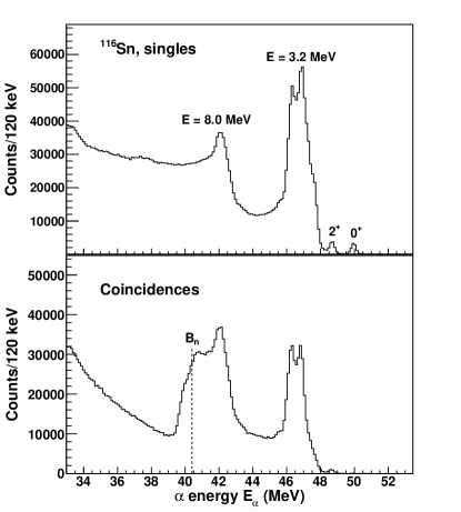
Figure 1: Singles $\alpha$-particle spectrum (upper panel), and $\alpha$-$\gamma$ coincidence spectrum (lower panel) from the ¹¹⁷Sn(³He, $\alpha$)¹¹⁶Sn reaction. The data are taken from the experiment presented in Ref. Sn_pairbreak .

Inside the CACTUS array, eight collimated Si particle detectors were used for detecting the charged ejectiles from the nuclear reactions. The particle detectors were placed at 45^∘ relative to the beam line in forward direction. The detectors were of $\Delta E-E$ type with a thin ($\sim 140$ $\mu$m) front detector and a thick ($\sim 1500$ $\mu$m) end detector where the charged ejectiles stop. The particle telescopes enable a good separation between the various charged-ejectile species. The energy resolution of the particle spectra ranges from $150-300$ keV depending on the beam species, the mass of the target nucleus and the size of the collimators. Both singles and coincidence events were measured for the ejectiles. In Figs. 1, 2 and 3 the singles and particle-$\gamma$ coincidence spectra are shown for the reactions ¹¹⁷Sn(³He,$\alpha$)¹¹⁶Sn, ¹⁶⁴Dy(³He,³He^′)¹⁶⁴Dy and ⁴⁶Ti($p$, $p^{\prime}$)⁴⁶Ti, respectively.

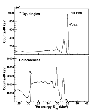
Figure 2: Singles ³He spectrum (upper panel), and ³He-$\gamma$ coincidence spectrum (lower panel) from the ¹⁶⁴Dy(³He,³He^′)¹⁶⁴Dy reaction. The data are taken from the experiment presented in Ref. hildes_DyRSF .

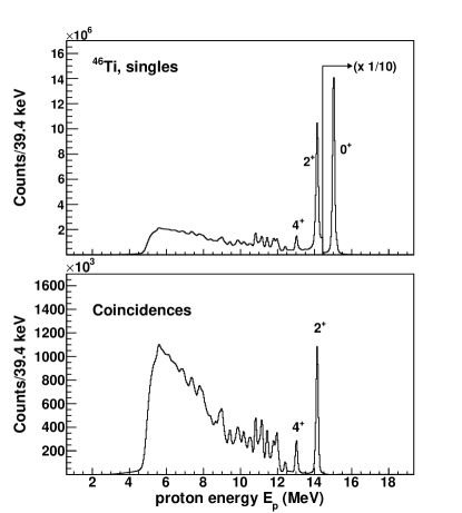
Figure 3: Singles proton spectrum (upper panel) and $p$-$\gamma$ coincidence spectrum (lower panel) from the ⁴⁶Ti($p$, $p^{\prime}$)⁴⁶Ti reaction. The data are taken from the experiment presented in Ref. magne_46Ti .

The ejectile energy can easily be transformed to the excitation energy of the residual nucleus using the reaction $Q$-values and kinematics. Thus, an excitation energy vs. $\gamma$-ray energy matrix can be built from the coincidence events. An example of such a matrix is shown in Fig. 4 (left panel), where the $\gamma$-ray spectra have been corrected for the known response functions of the CACTUS array Gut96 . The correction (or unfolding) method is described in detail in Ref. Gut96 . One of the main advantages with this method is that the fluctuations of the original spectra are preserved without introducing additional, spurious fluctuations.

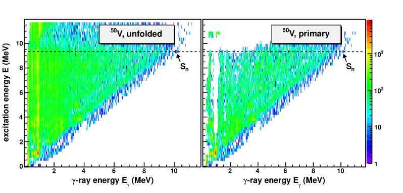
Figure 4: (Color online). Excitation-energy vs. $\gamma$-ray energy matrix (left), and primary $\gamma$-ray matrix (right) for ⁵⁰V. The data are taken from the experiment presented in Ref. V .

II.2 Extracting primary $\gamma$ rays

As $\gamma$ decay from highly excited states often involves a cascade of transitions, it is necessary to isolate the $\gamma$ rays that are emitted in the first decay step of all the possible decay routes, since information on the level density and the $\gamma$-ray strength function can be extracted from the distribution of these primary $\gamma$ rays (also called first-generation $\gamma$ rays). Therefore, a method has been developed in order to separate the primary $\gamma$-ray spectra from the $\gamma$ rays that origin from the later steps in the decay cascades at each excitation energy. This method will hereafter be referred to as the first-generation method and is described in detail in Ref. Gut87 . This method is very important, since the correctness of the further analysis is completely dependent on correctly determined primary $\gamma$-ray spectra. The first-generation method shares several features with another subtraction technique developed by Bartholomew et al. Bartholomew . The main features of the method will be outlined in the following.

From the $E$ vs. $E_{\gamma}$ matrix, where $\gamma$-ray spectra for each excitation energy are contained, the primary $\gamma$-ray spectra are extracted through an iterative subtraction technique. The unfolded spectra $f_{i}$ are made of all generations of $\gamma$ rays from all possible cascades decaying from the excited levels within the excitation-energy bin $i$. Now, we utilize the fact that the spectra $f_{j<i}$ for all the underlying energy bins $j$ contain the same $\gamma$-transitions as $f_{i}$ except the first $\gamma$ rays emitted, since they will bring the nucleus from the states in energy bin $i$ to underlying states in the bins $j$. Thus, the primary $\gamma$-ray spectrum $h_{i}$ for each bin $i$ can be found by

$$h_{i}=f_{i}-g_{i},$$ (1)

where $g_{i}$ is a weighted sum of all spectra

$$g_{i}=n_{i1}w_{i1}f_{1}+n_{i2}w_{i2}f_{2}+\ldots+n_{ij}w_{ij}f_{j}=\sum_{j}n_{ij}w_{ij}f_{j}.$$ (2)

Here, the unknown coefficients $w_{ij}$ (with the normalization $\sum_{j}w_{ij}=1$) represent the probability of the decay from states in bin $i$ to states in bin $j$. In other words, the $w_{ij}$ values make up the weighting function for bin $i$, and contain the distribution of branching ratios as a function of $\gamma$-ray energy. Therefore, the weighting function $w_{i}$ corresponds directly to the primary $\gamma$-ray spectrum $h_{i}$ for bin $i$.

The coefficients $n_{ij}$ are correcting factors for the different cross sections of populating levels in bin $i$ and the underlying levels in bin $j$. They are determined so that the total area of each spectrum $f_{i}$ multiplied by $n_{ij}$ corresponds to the same number of cascades. This can be done in two ways Gut87 :

• Singles normalization. The singles-particle cross section is proportional to the number of events populating levels in a specific bin, and thus to the number of decay cascades from this bin. We denote the number of counts measured for bin $i$ and $j$ in the singles spectrum $S_{i}$ and $S_{j}$, respectively. The normalization factor $n_{ij}$ that should be applied to the spectrum $f_{j}$ is then given by

  $$n_{ij}=\frac{S_{i}}{S_{j}}.$$ (3)

• Multiplicity normalization. The average $\gamma$-ray multiplicity $\langle M\rangle$ can be obtained in the following way Rekstad : Assume an $N$-fold population of an excited level $E$. The decay from this level will result in $N$ $\gamma$-ray cascades, where the $i$th cascade contains $M_{i}$ $\gamma$ rays. The average $\gamma$-ray energy $\langle E_{\gamma}\rangle$ is equal to the total energy carried by the $\gamma$ rays divided by the total number of $\gamma$ rays:

  $$\langle E_{\gamma}\rangle=N\cdot\frac{E}{\sum_{i=1}^{N}M_{i}}=\frac{E}{\frac{1}{N}\sum_{i=1}^{N}M_{i}}=\frac{E}{\langle M\rangle}.$$ (4)

  Then, the average $\gamma$-ray multiplicity is simply given by

  $$\langle M\rangle=\frac{E}{\langle E_{\gamma}\rangle}.$$ (5)

  The average $\gamma$-ray multiplicity $\langle M_{i}\rangle$ can thus easily be calculated for each excitation-energy bin $i$. Let the area (or total number of counts) of the $\gamma$-ray spectrum $f_{i}$ be denoted by $A(f_{i})$. Then the singles particle cross section $S_{i}$ is proportional to the ratio $A(f_{i})/\langle M_{i}\rangle$, and the normalization coefficient $n_{ij}$ that should be applied to bin $i$ when subtracting bin $j$ is

  $$n_{ij}=\frac{A(f_{i})/\langle M_{i}\rangle}{A(f_{j})/\langle M_{j}\rangle}=\frac{\langle M_{j}\rangle A(f_{i})}{\langle M_{i}\rangle A(f_{j})}.$$ (6)

The two normalization methods give normally the same results within the experimental error bars, see also Sec. III.2. The resulting primary $\gamma$-ray matrix of ⁵⁰V is shown in Fig. 4 (right panel), using the singles normalization method.

In cases where the multiplicity is well determined, an area consistency check can be applied to Eq. (1). Assume that a small correction is introduced by substituting $g_{i}$ by $\delta g_{i}$, where $\delta$ is close to unity. The area of the first-generation $\gamma$ spectrum is then

$$A(h_{i})=A(f_{i})-\delta A(g_{i}),$$ (7)

and this corresponds to a $\gamma$-ray multiplicity of one unit. Since the number of primary $\gamma$ rays in the spectrum $f_{i}$ equals $A(f_{i})/\langle M_{i}\rangle$, $A(h_{i})$ is also given by

$$A(h_{i})=A(f_{i})/\langle M_{i}\rangle.$$ (8)

Combining Eqs. (7) and (8) yields

$$\delta=(1-1/\langle M_{i}\rangle)\frac{A(f_{i})}{A(g_{i})}.$$ (9)

The $\delta$ parameter can be varied to get the best agreement of the areas $A(h_{i})$, $A(f_{i})$ and $A(g_{i})$ within the following restriction: $\delta=1.00\pm 0.15$; that is, the correction should not exceed 15%. If a larger correction is necessary, then improved weighting functions should be determined instead.

As mentioned before, the weighting coefficients $w_{ij}$ correspond directly to the first-generation spectrum $h_{i}$, and this close relationship makes it possible to determine $w_{ij}$ (and thus $h_{i}$) through a fast converging iteration procedure Gut87 :

1. Apply a trial function for $w_{ij}$.

2. Deduce $h_{i}$.

3. Transform $h_{i}$ to $w_{ij}$ by giving $h_{i}$ the same energy calibration as $w_{ij}$, and normalize the area of $h_{i}$ to unity.

4. If $w_{ij}$(new) $\approx$ $w_{ij}$(old), convergence is reached, and the procedure is finished. Otherwise repeat from step 2.

The first trial function could be the unfolded spectrum $f_{i}$, or a theoretical estimate based on a model for the level density and $\gamma$-ray transmission coefficient, or a constant function; it turns out that the resulting first-generation spectra are not sensitive to the starting trial function. Also, previous tests of the convergence properties of the procedure have shown that excellent agreement is achieved between the exact solution (from simulated spectra) and the trial function $w_{ij}$ already after three iterations Gut87 . Usually, about $10-20$ iterations are performed on experimental spectra.

II.3 Determining level density and $\gamma$-ray strength

Once the primary $\gamma$-ray spectra are obtained for each excitation energy, the first-generation matrix $P(E,E_{\gamma})$ is used for the determination of level density and $\gamma$-ray strength. For statistical $\gamma$-decay, the decay probability (given by $P(E,E_{\gamma})$) of a $\gamma$-ray with energy $E_{\gamma}$ decaying from a specific excitation energy $E$ is proportional to the level density $\rho(E_{\mathrm{f}})$ at the final excitation energy $E_{\mathrm{f}}=E-E_{\gamma}$, and the $\gamma$-ray transmission coefficient $\mathcal{T}(E_{\gamma})$:

$$P(E,E_{\gamma})\propto\rho(E_{\mathrm{f}}){\mathcal{T}}(E_{\gamma}).$$ (10)

The above relation holds for decay from compound states, which means that the relative probability for decay into any specific set of final states is independent on how the compound nucleus was formed. Thus, the nuclear reaction can be described as a two-stage process, where a compound state is first formed before it decays in a manner that is independent of the mode of formation BM ; hend1 . This is believed to be fulfilled at high excitation energy, even though direct reactions are used, as already discussed previously. Equation (10) can also be compared with Fermi’s golden rule:

$$\lambda=\frac{2\pi}{\hbar}\left|\left<\mathrm{f}\left|\hat{H}_{\mathrm{int}}\right|\mathrm{i}\right>\right|^{2}\rho(E_{\mathrm{f}}),$$ (11)

where $\lambda$ is the decay rate of the initial state $\left|\mathrm{i}\right>$ to the final state $\left|\mathrm{f}\right>$, and $\hat{H}_{\mathrm{int}}$ is the transition operator. In Eq. (10), an ensemble of initial and final states within each excitation-energy bin is considered, and thus we obtain here the average decay properties of a set of initial states to a set of final states. Note, however, that in contrast to Fermi’s golden rule where the matrix element is strictly dependent on the initial and final state, the transmission coefficient ${\mathcal{T}}$ is only dependent on the $\gamma$-ray energy and neither the initial nor the final excitation energy. This is in accordance with the Brink hypothesis brink , which states that the collective giant dipole mode built on excited states has the same properties as if built on the ground state. In its generalized form, this hypothesis includes all types of collective decay modes. Assuming that this hypothesis holds, the first-generation matrix $P(E,E_{\gamma})$ is separable into two functions $\rho$ and ${\mathcal{T}}$ as given in Eq. (10).

To extract the level density and the $\gamma$-ray transmission coefficient, an iterative procedure schi0 is applied to the first-generation matrix $P(E,E_{\gamma})$. The basic idea of this method is to minimize

$$\chi^{2}=\frac{1}{N_{\mathrm{free}}}\sum_{E=E^{\mathrm{min}}}^{E^{\mathrm{max}}}\sum_{E_{\gamma}=E_{\gamma}^{\mathrm{min}}}^{E}\left(\frac{P_{\mathrm{th}}(E,E_{\gamma})-P(E,E_{\gamma})}{\Delta P(E,E_{\gamma})}\right)^{2},$$ (12)

where $N_{\mathrm{free}}$ is the number of degrees of freedom, and $\Delta P(E,E_{\gamma})$ is the uncertainty in the experimental first-generation $\gamma$-ray matrix. The fitted first-generation $\gamma$-ray matrix $P_{\mathrm{th}}(E,E_{\gamma})$ can theoretically be approximated by

$$P_{\mathrm{th}}(E,E_{\gamma})=\frac{\rho(E-E_{\gamma}){\mathcal{T}}(E_{\gamma})}{\sum_{E_{\gamma}=E_{\gamma}^{\mathrm{min}}}^{E}\rho(E-E_{\gamma}){\mathcal{T}}(E_{\gamma})}.$$ (13)

The experimental matrix of first-generation $\gamma$ rays is normalized schi0 such that for every excitation-energy bin $E$, the sum over all $\gamma$ energies $E_{\gamma}$ from some minimum value $E_{\gamma}^{\mathrm{min}}$ to the maximum value $E_{\gamma}^{\mathrm{max}}=E$ at this excitation-energy bin is unity:

$$\sum_{E_{\gamma}=E_{\gamma}^{\mathrm{min}}}^{E}P(E,E_{\gamma})=1.$$ (14)

The experimental matrix $P(E,E_{\gamma})$ and the fitted matrix $P_{\mathrm{th}}(E,E_{\gamma})$ of ⁴⁶Ti are displayed in Fig. 5. The energy limits set in the first-generation matrix for extraction are also shown. These limits ($E^{\mathrm{min}}$, $E^{\mathrm{max}}$, and $E_{\gamma}^{\mathrm{min}}$) are chosen to ensure that the data utilized are from the statistical excitation-energy region and that no $\gamma$-lines stemming from, e.g., yrast transitions, are used in the further analysis. Note that the $\gamma$-ray energy bins are now re-binned to the same size (120 keV in this case) as the excitation-energy bins.

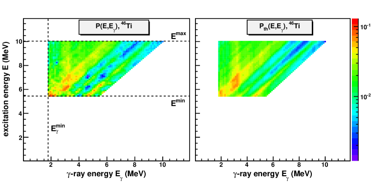
Figure 5: (Color online). Experimental first-generation matrix $P(E,E_{\gamma})$ (left) and the calculated $P_{\mathrm{th}}(E,E_{\gamma})$ (right) of ⁴⁶Ti from the iteration procedure of A. Schiller et al. schi0 . The dashed lines show the limits set in the experimental first-generation matrix for the fitting procedure. The data are taken from the experiment presented in Ref. magne_46Ti .

Each point of the $\rho$ and ${\mathcal{T}}$ functions is assumed to be an independent variable, so that the reduced $\chi^{2}$ of Eq. (12) is minimized for every argument $E-E_{\gamma}$ and $E$. The quality of the procedure when applied to ⁴⁶Ti and ¹⁶³Dy is shown in Figs. 6 and 7, where the experimental first-generation spectra for various initial excitation energies are compared to the least-$\chi^{2}$ solution. In general, the agreement between the experimental data and the fit is very good. Note, however, that differences of several standard deviations do occur. In the case of ⁴⁶Ti, this is particularly pronounced for the peaks at $E_{\gamma}\approx 4.7$ MeV for $E=5.6$ MeV and $E_{\gamma}\approx 5.5$ MeV for $E=6.4$ MeV. As these peaks correspond to the decay to the first excited state, one might expect large Porter-Thomas fluctuations porter-thomas in the strength of these transitions.

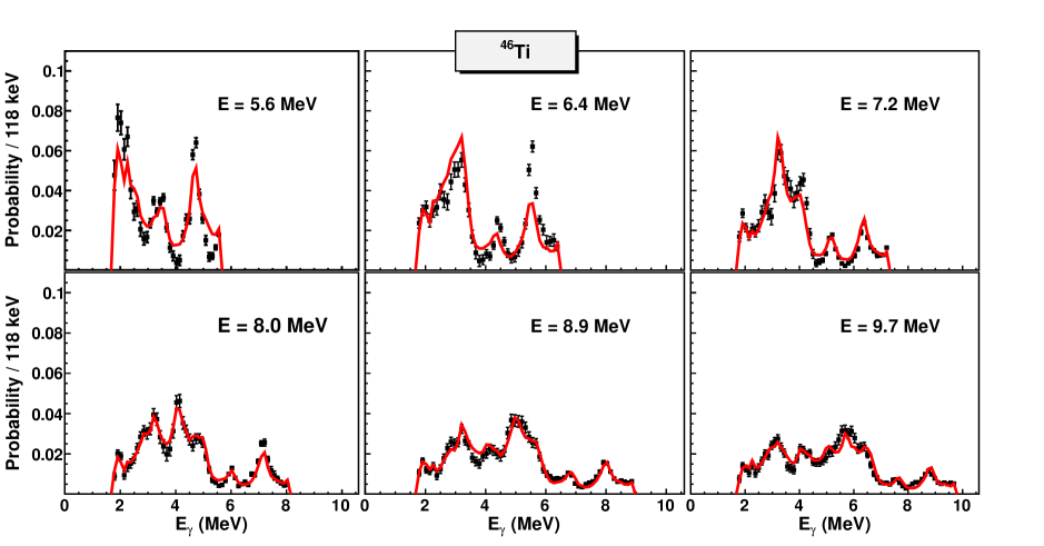
Figure 6: (Color online). Experimental first-generation $\gamma$ spectra (data points with error bars) at six different initial excitation energies (indicated in the figure) compared to the $\chi^{2}$ fit (solid lines) for ⁴⁶Ti. The fit is performed simultaneously on the entire first-generation matrix of which the six displayed spectra are a fraction. The data are taken from the experiment presented in Ref. magne_46Ti .

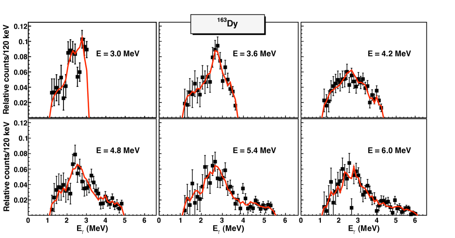
Figure 7: (Color online). Same as Fig. 6 for ¹⁶³Dy. The data are taken from the experiment presented in Ref. hildes_DyRSF .

The global fitting to the data points only gives the functional form of $\rho$ and ${\mathcal{T}}$. In fact, it has been shown schi0 that if one solution for the multiplicative functions $\rho$ and ${\mathcal{T}}$ is known, one may construct an infinite number of other functions, which give identical fits to the $P(E,E_{\gamma})$ matrix by

$$\tilde{\rho}(E-E_{\gamma}) = A\exp[\alpha(E-E_{\gamma})]\,\rho(E-E_{\gamma}),$$ (15)

$$\tilde{{\mathcal{T}}}(E_{\gamma}) = B\exp(\alpha E_{\gamma}){\mathcal{T}}(E_{\gamma}).$$ (16)

Therefore the transformation parameters $\alpha$, $A$ and $B$, which correspond to the physical solution, must be found from external data.

II.4 Normalization

In order to determine the correction $\alpha$ to the slope of the level density and the $\gamma$-ray transmission coefficient, and to determine the absolute value $A$ of the level density in Eq. (15), the $\rho$ function is adjusted to fit the number of known discrete levels at low excitation energy and neutron (or proton) resonance data at high excitation energy. This normalization is shown for ¹⁶⁴Dy in Fig. 8.

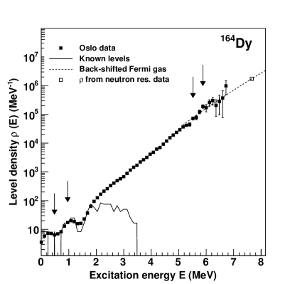
Figure 8: Normalization procedure of the level density (data points) of ¹⁶⁴Dy. The data points between the arrows are normalized to known levels at low excitation energy (solid line) and to the level density at the neutron separation energy (open square) using an interpolation with the Fermi-gas level density (dashed line). The data are taken from the experiment presented in Ref. hildes_DyRSF .

The data point at high excitation energy (open square in Fig. 8) is calculated in the following way according to Ref. schi0 . The starting point is Eqs. (4) and (5) of Ref. GC :

$$\rho(U,J)=\frac{\sqrt{\pi}}{12}\frac{{\rm exp}(2\sqrt{aU})}{a^{1/4}U^{5/4}}\frac{(2J+1)\exp\left[-(J+1/2)^{2}/2\sigma^{2}\right]}{2\sqrt{2\pi}\sigma^{3}},$$ (17)

and

$$\rho(U)=\frac{\sqrt{\pi}}{12}\frac{{\rm exp}(2\sqrt{aU})}{a^{1/4}U^{5/4}}\frac{1}{\sqrt{2\pi}\sigma},$$ (18)

where $\rho(U,J)$ is the level density for a given spin $J$, and $\rho(U)$ is the level density for all spins. The intrinsic excitation energy $U$, the level-density parameter $a$, and the spin cutoff parameter $\sigma$ are normally taken from Ref. egidy1 in previous works, or from Ref. egidy2 in recent works.

Now, let $I_{t}$ be the spin of the target nucleus in a neutron resonance experiment. The average neutron resonance spacing $D_{\ell=0}$ for s-wave neutrons can be written as

$$\frac{1}{D_{0}}=\frac{1}{2}\left[\rho(S_{n},J=I_{t}+1/2)+\rho(S_{n},J=I_{t}-1/2)\right],$$ (19)

because all levels with spin $J=I_{t}\pm 1/2$ are accessible in neutron resonance experiments, and because it is assumed that both parities contribute equally to the level density at the neutron separation energy $S_{n}$. Combining Eqs. (17)–(19) with $U=S_{n}$, one finds the total level density at the neutron separation energy to be

$$\rho(S_{n})=\frac{2\sigma^{2}}{D_{0}}\cdot\frac{1}{(I_{t}+1)\exp\left[-(I_{t}+1)^{2}/2\sigma^{2}\right]+I_{t}\exp\left[-I_{t}^{2}/2\sigma^{2}\right]}.$$ (20)

Note also that the resonance spacing between $p$-waves, $D_{1}$, could also be used for calculating $\rho(S_{n})$, see Ref. Pb .

Since our experimental data only reach up to excitation energies around $S_{n}-E_{\gamma}^{\mathrm{min}}$, an interpolation has been made between the Oslo data and $\rho(S_{n})$ using the back-shifted Fermi gas model of Refs. egidy1 ; egidy2 , as shown in Fig. 8. It should be noted that in most cases the gap between the data and $\rho(S_{n})$ is small, so that the normalization is not very sensitive to the interpolation; a pure exponential function of the type $\rho(E)=C_{0}\exp(C_{1}E)$, where $C_{0}$ and $C_{1}$ are fitting parameters, gives an interpolation of equally good agreement (see Ref. Heidi_Sn ).

The slope of the $\gamma$-ray transmission coefficient ${\mathcal{T}}(E_{\gamma})$ has already been determined through the normalization of the level density, as explained above. The remaining constant $B$ in Eq. (16) gives the absolute normalization of ${\mathcal{T}}$, and it is determined using information from neutron resonance decay on the average total radiative width $\langle\Gamma_{\gamma}\rangle$ at $S_{n}$ according to Ref. voin1 .

The starting point is Eq. (3.1) of Ref. Kopecky&Uhl_2 ,

$$\langle\Gamma_{\gamma}(E,J,\pi)\rangle= \frac{1}{2\pi\rho(E,J,\pi)}\sum_{XL}\sum_{J_{\mathrm{f}},\pi_{\mathrm{f}}}\int_{E_{\gamma}=0}^{E}{\mathrm{d}}E_{\gamma}{\mathcal{T}}_{XL}(E_{\gamma})$$

$$\times\rho(E-E_{\gamma},J_{\mathrm{f}},\pi_{\mathrm{f}}),$$ (21)

where $\langle\Gamma_{\gamma}(E,J,\pi)\rangle$ is the average total radiative width of levels with energy $E$, spin $J$ and parity $\pi$. The summation and integration are going over all final levels with spin $J_{\mathrm{f}}$ and parity $\pi_{\mathrm{f}}$ that are accessible through $\gamma$ transitions with energy $E_{\gamma}$, electromagnetic character $X$ and multipolarity $L$. Assuming that the main contribution to the experimental ${\mathcal{T}}$ is from dipole radiation ($L=1$), we get

$$B{\mathcal{T}}(E_{\gamma})=B\sum_{XL}{\mathcal{T}}_{XL}(E_{\gamma})\approx B\left[{\mathcal{T}}_{\mathrm{E1}}(E_{\gamma})+{\mathcal{T}}_{\mathrm{M1}}(E_{\gamma})\right],$$ (22)

from which the total, experimental $\gamma$-ray strength function can easily be calculated:

$$f(E_{\gamma})=\frac{1}{2\pi E_{\gamma}^{3}}B{\mathcal{T}}(E_{\gamma}),$$ (23)

from the relation between $\gamma$-ray strength function and $\gamma$-ray transmission coefficient RIPL :

$${\mathcal{T}}_{XL}(E_{\gamma})=2\pi E_{\gamma}^{(2L+1)}f_{XL}(E_{\gamma})\>.$$ (24)

Further, we also assume that there are equally many accessible levels with positive and negative parity for any excitation energy and spin, so that the level density is given by

$$\rho(E-E_{\gamma},J_{\mathrm{f}},\pm\pi_{\mathrm{f}})=\frac{1}{2}\rho(E-E_{\gamma},J_{\mathrm{f}}).$$ (25)

Now, by combining Eqs. (21), (22) and (25), the average total radiative width of neutron s-wave capture resonances with spins $I_{t}\pm 1/2$ expressed in terms of the experimental ${\mathcal{T}}$ is obtained:

$$\langle\Gamma_{\gamma}(S_{n},I_{t}\pm 1/2, \pi_{t})\rangle=\frac{B}{4\pi\rho(S_{n},I_{t}\pm 1/2,\pi_{t})}\int_{E_{\gamma}=0}^{S_{n}}\mathrm{d}E_{\gamma}\mathcal{T}(E_{\gamma})$$

$$\times\rho(S_{n}-E_{\gamma})\sum_{J=-1}^{1}g(S_{n}-E_{\gamma},I_{t}\pm 1/2+J),$$ (26)

where $I_{t}$ and $\pi_{t}$ are the spin and parity of the target nucleus in the $(n,\gamma)$ reaction, and $\rho(S_{n}-E_{\gamma})$ is the experimental level density. Note that the factor $1/\rho(S_{n},I_{t}\pm 1/2,\pi_{t})$ equals the neutron resonance spacing $D_{0}$. The spin distribution of the level density is assumed to be given by GC :

$$g(E,J)\simeq\frac{2J+1}{2\sigma^{2}}\exp\left[-(J+1/2)^{2}/2\sigma^{2}\right].$$ (27)

The spin distribution is normalized so that $\sum_{J}g(E,J)\approx 1$. The experimental value of $\langle\Gamma_{\gamma}\rangle$ at $S_{n}$ is then the weighted sum of the level widths of states with $I_{t}\pm 1/2$ according to Eq. (26). From this expression the normalization constant $B$ can be determined as described in Ref. voin1 . However, some considerations must be done before normalizing according to Eq. (26).

Methodical difficulties in the primary $\gamma$-ray extraction prevent determination of the function ${\mathcal{T}}(E_{\gamma})$ for $E_{\gamma}<E_{\gamma}^{\mathrm{min}}$ as discussed previously. In addition, the data at the highest $\gamma$-energies suffer from poor statistics. Therefore, ${\mathcal{T}}$ is extrapolated with an exponential function, as demonstrated for ⁵¹V in Fig. 9. The contribution of the extrapolation to the total radiative width given by Eq. (26) does not normally exceed $15$%, thus the errors due to a possibly poor extrapolation are of minor importance voin1 .

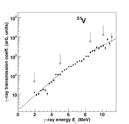
Figure 9: Extrapolation of the $\gamma$-ray transmission coefficient of ⁵¹V. The data points between the arrows in the low and high $\gamma$-energy regions are utilized to fit the exponential functions to the data. The data are taken from the experiment presented in Ref. V .

III Uncertainties and possible systematic errors

In the following, we will go through the Oslo method step by step with a close look at the uncertainties and possible systematic errors connected to it.

III.1 Unfolding of $\gamma$-ray spectra

The unfolding method is described in great detail in Ref. Gut96 . The method is based on a successive subtraction-iteration technique in combination with a special treatment of the Compton background. The stability of the method has been extensively tested in previous works and has proven to be very robust and reliable (see, e.g., Refs. V ; Sc ; Pb ). To some extent also the impact of slightly erroneous response functions has been investigated in Ref. hend1 . As this is the part of the method that has the largest potential of influencing the final results, it is further addressed here.

In the unfolding method, the $\gamma$-ray spectra are corrected for the total absorption efficiency of the NaI crystals for a given $\gamma$ energy. The applied efficiencies (normalized to the efficiency at 1.33 MeV) are shown in Fig. 10.

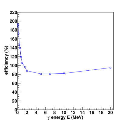
Figure 10: (Color online). Efficiencies relative to the 1.33-MeV efficiency used in the unfolding method.

We have tested the effect of reducing these efficiencies by up to $\approx 20$% for $\gamma$ energies above 1 MeV, using simulated particle-$\gamma$ coincidences generated with the DICEBOX code DICEBOX . In the DICEBOX algorithm, a complete decay scheme of an artificial nucleus is generated. In this case we have considered an artificial nucleus resembling ⁵⁷Fe. Below an excitation energy of about 2.2 MeV, all information from the known decay scheme is used; above this energy the levels and decay properties are generated from a chosen model of the level density and $\gamma$-ray strength function. The code allows to take into account Porter-Thomas fluctuations of the individual transition intensities as well as assumed fluctuations in the actual density of levels. Each particular set of the level scheme and the decay intensities is called a nuclear realization. For more details see Ref. DICEBOX . A restriction on the spin distribution of the initial excitation-energy levels of $1/2\leq J\leq 13/2$ was applied, and the chosen bin size was 120 keV. In these simulations, each level in a bin was populated with the same probability independently of its spin and parity. This means that Porter-Thomas fluctuations were not considered in the population of levels via the direct population, but only in the $\gamma$ decay.

The results on the extracted level density and $\gamma$-ray strength function are shown in Fig. 11.

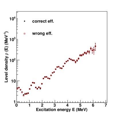
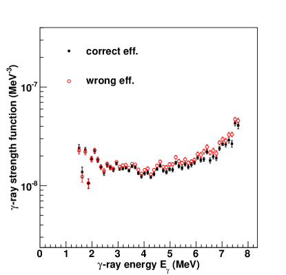
Figure 11: (Color online). Test of sensitivity on the total $\gamma$ efficiency on the level density (top) and $\gamma$-ray strength function (bottom) extracted from simulated data.

It is seen that the level density is not very sensitive to the total efficiency, but the slope of the $\gamma$-ray strength function is increased when using a too low efficiency for the high-energy $\gamma$ rays, thus leading to a too large correction in the unfolding procedure. However, it is very gratifying that the overall shape is indeed preserved, and the deviation in absolute value of the two $\gamma$-ray strength functions does not exceed 20%, corresponding to the maximum change in the absolute efficiency.

III.2 The first-generation method

The first-generation method, which is applied to extract the distribution of primary $\gamma$ rays from each excitation energy, is a sequential subtraction technique where an iterative procedure is applied to determine the weighting coefficients $w_{ij}$, which correspond to the primary $\gamma$-ray spectrum as described in Sec. II.2.

The main assumption of the first-generation method is that the $\gamma$ decay from any excitation-energy bin is independent on how the nucleus was excited to this bin. In other words, the decay routes are the same whether they were initiated directly by the nuclear reaction or by $\gamma$ decay from higher-lying states, giving rise to the same shape of the $\gamma$ spectra. This assumption is automatically fulfilled when states have the same cross section to be populated by the two processes, since $\gamma$ branching ratios are properties of the levels themselves.

In the region of high level density, the nucleus seems to attain a compound-like system before emitting $\gamma$ rays even though direct reactions are utilized. This is due to two factors. First, a significant configuration mixing of the levels will appear when the level spacing is comparable to the residual interaction. Second, the reaction time, and thus the time it takes to create a complete compound state, is $\approx 10^{-18}$s, while the typical life time of states in the quasi-continuum is $\approx 10^{-15}$s. Therefore, it is reasonable to assume that the nucleus has thermalized prior to $\gamma$ decay. This is supported by recent calculations betac based on the Iwamoto-Harada-Bispinghoff model, showing that for the ¹⁶⁰Dy(³He,$\alpha\gamma$) reaction with a 45-MeV ³He beam, the pre-equilibrium (”direct”) component of the $\gamma$-ray spectra is very small for $\gamma$ energies below $\approx 10$ MeV (see Fig. 12). The same is true for the ⁴⁶Ti($p,p^{\prime}\gamma$) reaction with proton beam energy $E_{p}=15$ MeV, see Fig. 13. Note that the ”direct” component is calculated using the pre-equilibrium (i.e. statistical) formalism.

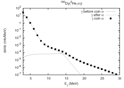
Figure 12: Calculated $\gamma$-ray spectra from the ¹⁶⁰Dy(³He,$\alpha\gamma$) reaction at 45 MeV betac . The solid line shows the pre-equilibrium component of the total $\gamma$-ray spectrum ($\gamma$ before $\alpha$), the dashed line represents the equilibrium part ($\alpha$ before $\gamma$), and the filled squares give the total spectrum.

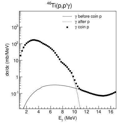
Figure 13: Same as Fig. 12, but for the inelastic scattering ⁴⁶Ti($p,p^{\prime}\gamma$) at $E_{p}=15$ MeV.

Experimentally, the independence of the reaction mechanism has been tested by creating the same compound nucleus with the two different reactions (³He,$\alpha$) and (³He,³He’). This has been done for, e.g., ^96,97Mo Mo_RSF , ^161,162Dy bagheri , and ^171,172Yb undraa . One observes an excellent agreement with the level density and $\gamma$-ray strength function resulting from the two reactions within the experimental error bars. However, at very low excitation energies, there is a significant difference in the obtained level density: the inelastic scattering gives consistently a higher level density close to the ground state than does the pick-up reaction. This could be a sign that the inelastic scattering populates states with wave functions having a large overlap with the ground state and the low-lying excited states. Thus, the decay to the ground state and low-lying states will be very fast, and cannot be characterized as compound decay.

The region at low excitation energies can be tricky also in other aspects. Vertical ridges and/or valleys can occur in the primary $\gamma$-ray matrix as a consequence of differences in feeding of these discrete states, giving significantly different shapes of the $\gamma$ spectra at low $E$ compared to higher excitation energies. The direct reaction cross section depends strongly on the intrinsic wave functions of low lying states, as seen in the particle spectra in Figs. 1–3. One can encounter the situation where some of these states are very weakly populated in the reaction, but strongly fed through decay from above-lying states. This means that some higher-order $\gamma$ rays are not fully subtracted in the first-generation method, giving an erroneous primary $\gamma$-ray spectrum for low $E_{\gamma}$. On the other hand, the reaction might populate very strongly some low-lying states that are more moderately populated by decay from above. One can then subtract too much of the $\gamma$ rays from these states.

The latter case is demonstrated for ⁵⁰V in the right panel of Fig. 4. A state at excitation energy 910 keV with spin/parity 7⁺ decaying 100% to the ground state, is strongly populated in the neutron pick-up reaction, which favors high-$\ell$ transfer (here $\ell=3$, see Ref. V50_spec ). However, it is not so strongly populated by $\gamma$ decay from above, and the result is that there is a vertical valley with zero counts in the primary $\gamma$-ray matrix at this $\gamma$ energy.

Furthermore, it is important that the populated spin distribution is (at least approximately) independent on the excitation energy. Else, the bins at high excitation energy will contain decay from states with higher spin than the bins at lower excitation energy, again disturbing the low-energy part of the primary $\gamma$-ray spectra. For the ¹⁶³Dy(³He, $\alpha$)¹⁶²Dy reaction, the spin population has been extensively studied in Ref. hend1 and references therein. In this specific case, the spin distribution turned out to be approximately constant in the excitation-energy region investigated. Also, for the lighter nuclei it is observed that indeed, the spins are populated with the same relative intensities within the error bars. This is seen for ⁵⁰V in the left panel of Fig. 4: the relative feeding to the low-lying states (vertical lines) is approximately the same for the whole quasi-continuum region. This is also the case for ⁴⁶Ti magne_46Ti .

Another potential problem could arise from the finite detector resolution. To illustrate this, consider a first-generation $\gamma$-ray of 8 MeV, decaying from $E_{i}=10$ MeV to $E_{f}=2$ MeV. This $\gamma$-ray would typically have a resolution of $\approx 250$ keV, while the particle resolution could be $\approx 150$ keV (for 15-MeV protons). This means that the weighting function (see Sec. II.2) for $E_{f}=2$ MeV is about 100 keV broader than the excitation-energy resolution at this point. If the situation is that there is only one level within $E_{f}$, one could then ”miss” some of the weighting function because it is broader than the particle peak. It could also be that the opposite situation applies: low-energy $\gamma$ rays with, say, 50-keV resolution might decay to excitation energies with resolution ranging from $150-300$ keV, leading to too narrow weighting functions.

We have tested the effects of different resolutions by employing a very simple, artificial decay scheme, see Fig. 14. A hypothetical nucleus with three excited states at $E_{1}=3.5$ MeV, $E_{2}=6$ MeV, and $E_{3}=8$ MeV, was assumed to have the following decay scheme:

• from $E_{3}$: 30% $\gamma_{a}$, 20% $\gamma_{b}$, and 50% $\gamma_{c}$.

• from $E_{2}$: 67% $\gamma_{d}$, and 33% $\gamma_{e}$.

• from $E_{1}$: 100% $\gamma_{f}$.

The $\gamma$-ray energies involved are: $\gamma_{a}=2.0$ MeV, $\gamma_{b}=4.5$ MeV, $\gamma_{c}=8.0$ MeV, $\gamma_{d}=2.5$ MeV, $\gamma_{e}=6.0$ MeV, and $\gamma_{f}=3.5$ MeV. The first-generation $\gamma$ rays from $E_{3}$ are then $\gamma_{a}$, $\gamma_{b}$, and $\gamma_{c}$, from $E_{2}$ $\gamma_{d}$ and $\gamma_{e}$, and from $E_{1}$ $\gamma_{f}$.

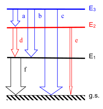
Figure 14: (Color online). Hypothetical decay scheme of an artificial nucleus (see text).

Applying no smoothing for all excitation energies, i.e., the $\gamma$-ray peaks are $\delta$ functions, the exact result is obtained from the first-generation method. Then, we assume 200-keV resolution for all excitation energies, but with an energy-dependent resolution of the $\gamma$-ray spectrum with 50-keV resolution for 1-MeV $\gamma$ rays and 300-keV resolution for 9-MeV $\gamma$ rays, similar to the experimental conditions. This constructed matrix is shown in Fig. 15.

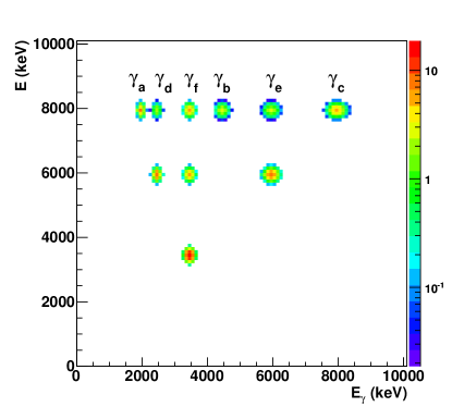
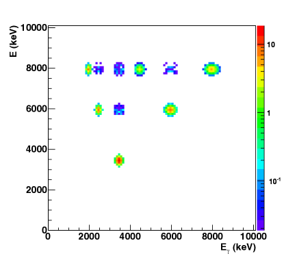
Figure 15: (Color online). Matrix of energy levels and $\gamma$ transitions in an artificial nucleus. Top: original matrix; bottom: result after the first-generation method is applied.

When applying the first-generation method on this smoothed matrix, we get the result shown in the lower part of Fig. 15. It is seen that it is not exact any more, but the differences are small. For example, for $E_{3}=8$ MeV, $\gamma_{d}$ is not a primary transition and should have been completely gone in the first-generation spectrum, but still about 5% of the counts in the original peak is present. For the $\gamma_{e}$ and $\gamma_{f}$ peaks, the situation is the same; also so for $\gamma_{f}$ at $E_{2}=6$ MeV. This means that one might expect leftovers of higher-generation $\gamma$ rays of the order of 5% in the primary spectra. Compared to values of experimental errors, which are typically within $5-30$%, this is a relatively small effect (the error propagation is discussed in detail in Ref. schi0 ).

To check more thoroughly what effect possible errors in the first-generation method might have on the final results, namely the extracted level density and strength function, we have performed simulations with the generalized version of DICEBOX DICEBOX , as already discussed biefly in Sec. III.1. Again, we have considered an artificial nucleus resembling ⁵⁷Fe, with a spin distribution of the initial excitation-energy levels of $1/2\leq J\leq 13/2$, and bin size of 120 keV. Note also that equally many negative- and positive-parity states are assumed above the region of known, discrete levels.

First, the simulated spectra were folded with the CACTUS response functions, and also a Gaussian smoothing was applied giving a full width at half maximum (FWHM) of 250 keV for all excitation energies. These spectra were thus made to be as similar as possible to experimental spectra. Then, we applied the unfolding technique and the first-generation method to obtain the first-generation spectra. We then compared the extracted first-generation matrix with the true first-generation matrix from the simulations, after smoothing the true first-generation spectra with a resolution similar to the experimental one. Examples of two such matrices for one nuclear realization are shown in Fig. 16.

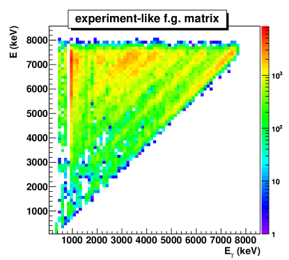
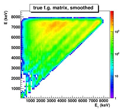
Figure 16: (Color online). Simulated first-generation matrix for ⁵⁷Fe. Top: spectra from folded data set. Bottom: true spectra with smoothing similar to the experimental resolution.

The overall good similarity between the two matrices is gratifying. However, in the low-$E_{\gamma}$ region, there are significant differences between the results extracted from the experiment-like matrix and the true, smoothed matrix. In particular, one can see that there are some vertical lines in the experiment-like first-generation matrix, e.g., for $E_{\gamma}\approx$1020 keV, that are not present in the true matrix. This particular vertical ridge originates from the 7/2^- state at 1007 keV, which for this nuclear realization is strongly populated in the decay cascades at high excitation energy. However, at low excitation energies, which corresponds to the population from the direct reaction, this state is only moderately populated. Thus, its $\gamma$ decay is not correctly subtracted in the first-generation procedure. It is therefore important to exclude such leftovers from higher-generation $\gamma$ rays in the further analysis, as mentioned in Sec. II.3.

We also tested the case with a Gaussian smoothing on the particle resolution, and the ideal response on the $\gamma$-detection side. The extracted level densities and strength functions for all three cases are displayed in Fig. 17.

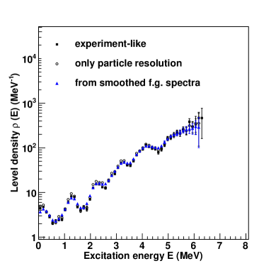
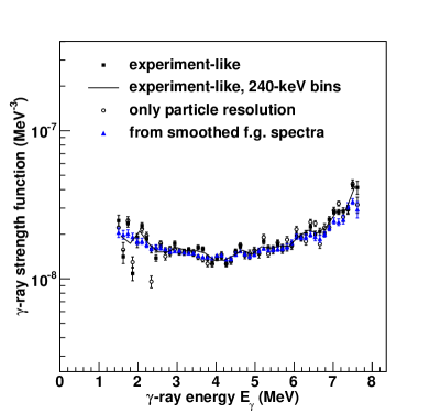
Figure 17: (Color online). Results from simulated spectra on ⁵⁷Fe. Top: level density. Bottom: $\gamma$-ray strength function.

In general, the results agree very well. We note that there are larger fluctuations in the strength function extracted from the experiment-like matrix as well as the case where only the particle resolution is applied, especially in the region below $E_{\gamma}\approx 2.5$ MeV. These fluctuations are related to uncertainties in the first-generation subtraction procedure and could be due to small variations in the shape of the $\gamma$ spectra. However, by compressing the experiment-like $\gamma$ spectra by a factor of two (bin size of 240 keV), we obtain practically the same shape of the $\gamma$-ray strength function as from the true first-generation spectra (see Fig. 17).

Finally, we have tested the two normalization options (singles or multiplicity) of the first-generation method on experimental spectra to investigate the effect on the extracted level density and $\gamma$-ray strength function. The result for ⁵¹V is shown in Fig. 18.

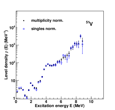
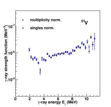
Figure 18: (Color online). Test of the two normalization options in the first-generation method for ⁵¹V. Top: level density. Bottom: $\gamma$-ray strength function. The data are taken from the experiment presented in Ref. V .

We observe that the two options give very similar results, only a very few data points are outside the experimental error bars. It is clear that the two methods do not give any difference in the overall shape of neither the level density nor the strength function.

III.3 The Brink hypothesis

The $\gamma$-ray transmission coefficient $\mathcal{T}(E_{\gamma})$ in Eq. (10) is assumed to be independent of excitation energy (and thus nuclear temperature) according to the generalized Brink hypothesis brink , as discussed in Sec. II.3. This hypothesis is violated when high temperatures and/or spins are involved in the nuclear reactions, as shown for giant dipole excitations (see Ref. Andreas&Thoennessen and references therein). However, since both the temperature reached and the spins populated are rather low for the Oslo experiments, these dependencies are usually assumed to be of minor importance in the relatively low excitation-energy region considered here.

The effect of the Brink hypothesis has been tested by analyzing simulated spectra on an artificial nucleus resembling ¹⁶³Dy. The simulations were again performed with the DICEBOX code DICEBOX for a specific spin range on the initial excited levels, $1/2\leq J\leq 13/2$.

As a first step, a temperature-independent model for the $\gamma$-ray strength function was used as input for the simulations. The extracted and input $\gamma$-ray strength function are shown in Fig. 19. As expected, the Oslo method works very well in this case.

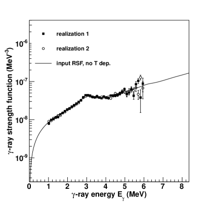
Figure 19: Results from simulated spectra of the artificial nucleus ¹⁶³Dy. The extracted $\gamma$-ray strength functions are shown as black points and open circles for two different nuclear realizations, while the input $\gamma$-ray strength model is shown as a solid line.

In the next test, a temperature-dependent input $\gamma$-ray strength function was used, with temperature $T\propto\sqrt{E_{\mathrm{f}}}$. In principle, it is not possible to disentangle the input level density and $\gamma$-ray strength function anymore, since now we have

$$P(E,E_{\gamma})\propto\rho(E_{\mathrm{f}}){\mathcal{T}}(E_{\mathrm{f}},E_{\gamma}).$$ (28)

This we keep in mind when we use the procedure of Ref. schi0 in order to extract the level density and $\gamma$-ray strength function.

The extracted $\gamma$-ray strength functions for two different nuclear realizations are shown in Fig. 20, within the excitation-energy range $2.1<E<6.2$ MeV.

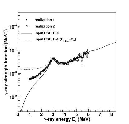
Figure 20: Results from simulated spectra of ¹⁶³Dy. The extracted $\gamma$-ray strength functions are displayed as black and open squares for two different nuclear realizations. The input $\gamma$-ray strength function models for $T_{f}=0$ (solid line) and $T_{f}\propto\sqrt{(S_{n}-E_{\gamma})}$ (dashed-dotted line) are also shown.

It is seen that the extracted $\gamma$-ray strength function lies in between the two extremes of the temperature-dependent input model, and thus an average strength function for the excitation energy region under study is found. The shape of the extracted $\gamma$-ray strength function is therefore quite reasonable, although it is clear that the low-energy part with $1\leq E_{\gamma}\leq 2.5$ MeV must necessarily be quite different from the two extremes of the input.

This is further illustrated in Fig. 21, where we have extracted the $\gamma$-ray strength function for two separate excitation-energy regions: $2.1<E<4.1$ MeV and $4.1<E<6.2$ MeV.

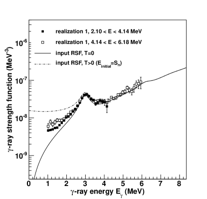
Figure 21: Results from simulated spectra of the artificial nucleus ¹⁶³Dy. The extracted $\gamma$-ray strength functions for two excitation-energy regions are displayed as black and open squares. The input $\gamma$-ray strength function models for $T_{f}=0$ (solid line) and $T_{f}\propto\sqrt{(S_{n}-E_{\gamma})}$ (dashed-dotted line) are also shown.

It is easily seen that the $\gamma$-ray strength function for $\gamma$ energies between $\approx 1-2$ MeV is different in the two cases; the higher excitation energies lead to a higher temperature of the final states and thus a higher strength function.

However, one should keep in mind that the experimental $\gamma$-ray strength functions have been tested against the assumption of temperature dependence for many nuclei, e.g., ⁴⁵Sc Sc , ^56,57Fe Fe_Alex , ^96,98Mo Mo_RSF , and ¹¹⁷Sn Sn_RSF . This is also shown for ¹⁶⁴Dy hildes_DyRSF in Fig. 22, where the $\gamma$-ray strength function has been extracted for three sets of initial excitation energies. As can be seen from the figure, the similarity of the three $\gamma$-ray strength functions is striking.

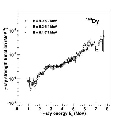
Figure 22: Experimental $\gamma$-ray strength function of ¹⁶⁴Dy for three sets of initial excitation energies. The data are taken from the experiment presented in Ref. hildes_DyRSF .

There is, therefore, no experimental evidence in this excitation-energy region for a strong temperature dependence in the strength function. Hence, the Brink hypothesis seems to be valid here.

III.4 The parity distribution

As mentioned previously, for both the normalization of the level density and the $\gamma$-ray transmission coefficient, the assumption of equally many levels with positive and negative parity is used. We will in the following investigate this assumption in detail.

Using $\rho_{+}$ and $\rho_{-}$ to denote the level density with positive and negative parity levels, the parity asymmetry $\alpha$ is defined as gary

$$\alpha=\frac{\rho_{+}-\rho_{-}}{\rho_{+}+\rho_{-}},$$ (29)

which gives $-1$ and $1$ for only negative and positive parities, respectively, and 0 when both parities are equally represented.

Another expression widely used in literature is the ratio $\rho_{-}/\rho_{+}$, which relates to $\alpha$ by

$$\frac{\rho_{-}}{\rho_{+}}=\frac{1-\alpha}{1+\alpha}.$$ (30)

We have considered theoretical parity distributions from combinatorial plus Hartree-Fock-Bogoliubov calculations of spin- and parity-dependent level densities go08 . Applying the definition in Eq. (29), we find the calculated parity distributions for several Fe, Mo, and Dy isotopes as shown in Figs. 23–25. As one might expect from the fact that more orbits are accessible at increasing excitation energy, the parity distributions are seen to approach zero as the excitation energy increases. However, it is clear that for the lighter nuclei, in particular the Fe isotopes, the assumption of zero parity asymmetry is not fulfilled in the calculations for excitation energies below $\approx 10$ MeV.

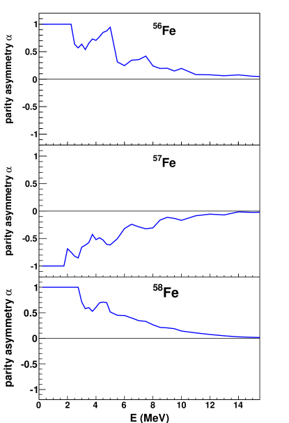
Figure 23: (Color online). Calculated parity distributions as a function of excitation energy calculated for ^56-58Fe, from Ref. go08 .

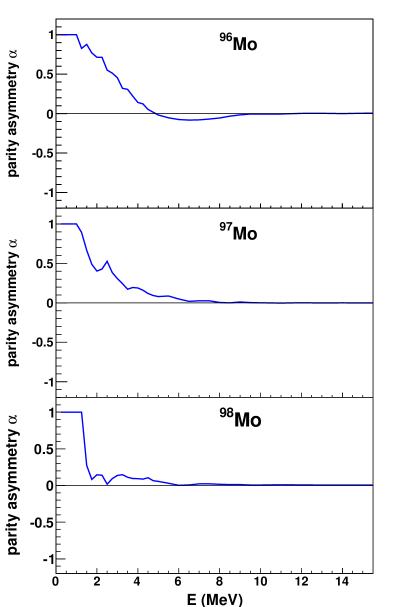
Figure 24: (Color online). Same as Fig. 23 for ^96-98Mo.

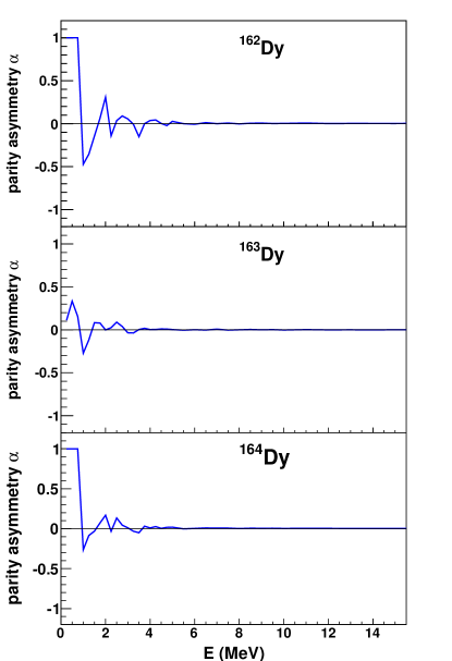
Figure 25: (Color online). Same as Fig. 23 for ^162-164Dy.

We have also looked at other theoretical work such as shell-model Monte Carlo calculations Alhassid and macroscopic-microscopic calculations Rauscher . In Fig. 2 of Ref. Rauscher , the ratio $\rho_{-}/\rho_{+}$ is shown for ⁵⁶Fe, indicating a value of $\rho_{-}/\rho_{+}\simeq 0.1$ at 10 MeV excitation energy. From Fig. 4 in Ref. Alhassid , the ratio $\rho_{-}/\rho_{+}\simeq 0.2$ for $E=10$ MeV. In contrast to this, the combinatorial calculations of Ref. go08 give $\rho_{-}/\rho_{+}\simeq 0.7$ at $E=10$ MeV, which is also in accordance with other microscopic calculations based on the Nilsson model and BCS quasi-particles Fe_Emel , where $\rho_{-}/\rho_{+}\simeq 0.5$. These results indicate considerably more negative-parity states in ⁵⁶Fe than found in Refs. Alhassid ; Rauscher . In this specific case, the amount of positive-parity states is very sensitive to the position of the $g_{9/2}$ orbital relative to the Fermi level.

To our understanding, there are currently no experimental data on the parity distribution in ⁵⁶Fe. However, recent measurements on level densities of $J^{\pi}=2^{+}$ and $2^{-}$ states in ⁵⁸Ni and ⁹⁰Zr vonNeumann-Cosel show no indication of a significantly larger amount of states with one of the parities in none of the nuclei under study at $E\approx 10$ MeV. Also, from the study of proton resonances in ⁴⁵Sc gary , equally many $1/2^{+}$ and $1/2^{-}$ states were found, again at $E\approx 10$ MeV. Thus it seems reasonable to assume that the parity asymmetry is at least very small for these excitation energies, in support of the assumption of equal parity as described in Sec. II.4.

We would nevertheless like to investigate the impact of the assumption of parity symmetry on the calculations of $\rho(S_{n})$. Let us assume that the spin- and parity-projected level density $\rho(E,J,\pi)$ can be described by Rauscher

$$\rho(E,J,\pi)=\rho(E)\cdot g(E,J)\cdot\mathcal{P}(E,\pi),$$ (31)

where $\rho(E)$ is the total level density at excitation energy $E$, $g(E,J)$ is the spin distribution given by Eq. (27), and $\mathcal{P}(E,\pi)$ is the parity projection factor. According to Eq. (19), we get

$$\frac{1}{D_{0}}=\rho(S_{n})\cdot g(S_{n},J=I_{t}\pm 1/2)\cdot\mathcal{P}(S_{n},\pi_{t})$$ (32)

for the neutron resonance spacing at $S_{n}$ reaching states with parity $\pi_{t}\cdot(-1)^{\ell}=\pi_{t}$ for s-wave neutrons having $\ell=0$. Now, we define the parity projection factor for positive and negative parities as

$$\mathcal{P}_{+}\equiv\mathcal{P}(E,\pi=\pi_{+})=\frac{\rho_{+}}{\rho}=\frac{1+\alpha}{2},\\$$ (33)

and

$$\mathcal{P}_{-}\equiv\mathcal{P}(E,\pi=\pi_{-})=\frac{\rho_{-}}{\rho}=\frac{1-\alpha}{2},$$ (34)

using

$$\mathcal{P}_{+}+\mathcal{P}_{-}=1.$$ (35)

Further,

$$\frac{1}{D_{0}} =\rho(S_{n})\left[g(S_{n},J=I_{t}+1/2)+g(S_{n},J=I_{t}-1/2)\right]\mathcal{P}(S_{n},\pi)$$ (36)

$$=\rho(S_{n})\left[g(S_{n},J=I_{t}+1/2)+g(S_{n},J=I_{t}-1/2)\right]\frac{1\pm\alpha}{2},$$ (37)

which gives

$$\rho(S_{n})=\frac{\sigma^{2}}{D_{0}}\frac{(1\pm\alpha)/2}{(I_{t}+1)\exp\left[-(I_{t}+1)^{2}/2\sigma^{2}\right]+I_{t}\exp\left[-I_{t}^{2}/2\sigma^{2}\right]},$$ (38)

using Eq. (27). If the target nucleus in the neutron-capture experiment has positive parity in the ground state, the factor $(1+\alpha)/2$ is used, and for negative ground-state parity we use $(1-\alpha)/2$.

For several key cases, we have applied Eq. (38) for calculating $\rho(S_{n})$ and compared to the result using Eq. (20). For example, for ⁵⁸Fe with neutron resonance spacing $D_{0}=6.5$ keV at $S_{n}=10.044$ MeV RIPL , and using the spin cutoff parameter $\sigma(S_{n})=3.93$ from the prescription of Ref. egidy2 , we obtain $\rho(S_{n})=2518$ MeV^-1 if the assumption of equal parity is used, and $\rho(S_{n})=2939$ MeV^-1 if we correct for the parity asymmetry $\alpha=0.14$ predicted by the combinatorial model of go08 . Thus, including the parity asymmetry gives about 17% higher level density at $S_{n}$. For ⁹⁶Mo, with $D_{0}=105$ eV RIPL , $\sigma(S_{n})=5.15$, and $\alpha=-0.017$ go08 , we get $\rho(S_{n})=1.01\cdot 10^{5}$ MeV^-1 when no parity asymmetry is taken into account, and $\rho(S_{n})=1.03\cdot 10^{5}$ MeV^-1 when the parity asymmetry is considered; only a change of $\approx 2$%.

To check the effect of the parity asymmetry on the normalization, we have renormalized the data on ⁹⁶Mo using the above-mentioned values for $\rho(S_{n})$ with and without parity correction. Since the estimated $\alpha$ was so small for this case, we have also assumed a much larger parity asymmetry of $\alpha=-0.5$ leading to $\rho(S_{n})=2.02\cdot 10^{5}$ MeV^-1, a factor of 2 larger level density than the one assuming equal parity. Assuming that $\alpha=0.5$ gives $\rho(S_{n})=6.74\cdot 10^{4}$ MeV^-1, roughly a factor of 2/3 reduction compared to the parity-symmetry case.

The resulting level density and strength function are shown in Figs. 26.

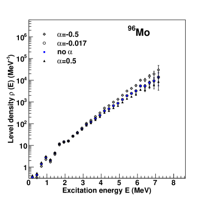
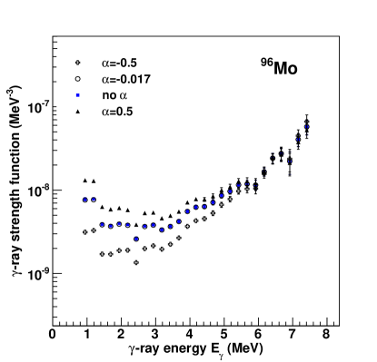
Figure 26: (Color online). Effect of parity asymmetry on the experimental level density (upper panel) and strength function (lower panel) of ⁹⁶Mo. The data are taken from the experiment presented in Ref. Mo_RSF .

Here, it is easily seen that a small parity asymmetry does not give any significant changes of the normalization in neither the level density nor the strength function. However, for $\alpha=-0.5$ corresponding to a factor of 2 larger $\rho(S_{n})$ gives an overall larger level density for excitation energies larger than $\approx 3$ MeV, and the steeper slope is reflected also in the strength function. In addition, one sees a suppression in the $\gamma$-ray strength function for $E_{\gamma}\lesssim 6$ MeV, a direct consequence of the changes in the level density. The opposite is true for $\alpha=0.5$; here, $\rho(S_{n})$ and thus the slope of the level density is reduced. Consequently, the slope is reduced also in the $\gamma$-ray strength function, but the absolute value for $E_{\gamma}\lesssim 6$ MeV is in this case increased with respect to the parity-symmetry case. Note that such large values of $\alpha$ represent extreme cases; both from experimental data gary ; vonNeumann-Cosel and several theoretical estimates (e.g, go08 ; Fe_Emel ) the asymmetry around $S_{n}$ should be smaller than typically $\pm 0.2$.

The assumption of parity symmetry influences also the normalization of the $\gamma$-ray transmission coefficient. To take into account the parity distribution, one can modify Eq. (25) according to Eq. (31) so that

$$\rho(E-E_{\gamma},J_{\mathrm{f}},\pi_{\mathrm{f}})=\rho(E-E_{\gamma})\cdot\mathcal{P}(E-E_{\gamma},\pi_{\mathrm{f}})\cdot g(E-E_{\gamma},J_{\mathrm{f}}).$$ (39)

We will restrict ourselves to consider $\ell=1$ radiation only ($E1$ and $M1$), since in general, this multipolarity is expected to give by far the largest contribution to the strength function in the quasicontinuum region (see, e.g., studies by Kopecky and Uhl Kopecky&Uhl_2 ).

For $E1$ radiation, the parity of the final state is opposite to the initial state. In s-wave neutron capture experiments, the parity of the target nucleus’ ground state is equal to the parity of the neutron resonances of the created compound nucleus. Therefore, the accessible parity of the final states must be the opposite of the initial state. For $M1$ radiation, the accessible final states must have the same parity as the initial state.

Based on Eq. (21) and taking the parity distribution into account, one finds

$$\langle\Gamma_{\gamma}(S_{n},I_{t}\pm 1/2,\pi_{t})\rangle=\frac{B}{2\pi\rho(S_{n},I_{t}\pm 1/2,\pi_{t})}$$

$$\times\int_{E_{\gamma}=0}^{S_{n}}\mathrm{d}E_{\gamma}\left[\mathcal{T}_{E1}(E_{\gamma})\mathcal{P}_{-/+}+\mathcal{T}_{M1}(E_{\gamma})\mathcal{P}_{+/-}\right]$$

$$\times\rho(S_{n}-E_{\gamma})\sum_{J=-1}^{1}g(S_{n}-E_{\gamma},I_{t}\pm 1/2+J).$$ (40)

for target nuclei with positive/negative ground-state parity. It is easily seen that if $\mathcal{P}_{+}=\mathcal{P}_{-}=1/2$, Eq. (26) is restored.

The Oslo method does not enable the separation of $\mathcal{T}(E_{\gamma})$ into its $E1$ and $M1$ components. We have therefore applied models for the level density and the $E1$ and $M1$ strength functions in order to investigate the influence of including parity on the integral in Eq. (40). For the level density, we have used the results of go08 . For the $E1$ strength function, we have used the the Kadmenskiĭ, Markushev and Furman (KMF) model ka83 with a constant temperature $T_{f}=0.3$ MeV, while for the $M1$ component (the spin-flip resonance BM ) we have applied a Lorentzian shape (see Ref. RIPL ). We use again ⁹⁶Mo as a test case, with experimental GDR parameters taken from Ref. RIPL and $M1$ Lorentzian parameters from systematics RIPL . The target nucleus ⁹⁵Mo in the $(n,\gamma)^{96}$Mo reaction has spin/parity $5/2^{+}$.

First, we take the parity distribution from Ref. go08 as shown in Fig. 24 and apply in the integral of Eq. (40). The resulting value is only about 1% smaller than the value obtained assuming $\mathcal{P}_{+}=\mathcal{P}_{-}=1/2$ for all excitation energies, implying that the effect of parity is negligible in this case. As a further test we used the parity distribution of ⁵⁶Fe shown in Fig. 23 on ⁹⁶Mo; then, we found a $\approx 47$% reduction using Eq. (40) compared to the parity-symmetry case. For the very extreme cases assuming that $\alpha=1$ for all $E$ (allowing only for positive-parity states and $M1$ transitions), we get about a factor of 3 reduction, and using $\alpha=-1$ for all $E$ (allowing only for negative-parity states and $E1$ transitions), we obtain about 67% increase of the normalization integral in Eq. (40) relative to the case where no parity distribution is considered.

To summarize, for nuclei in the Mo mass region and above, we find only small corrections of the order of a few percent to the estimation of $\rho(S_{n})$ and also for the absolute normalization of the strength function when using realistic parity distributions (compared to the extreme cases). However, for light nuclei such as Fe, effects of the parity distribution could be significant on both the level-density and strength-function normalization, of the order of 30–50%.

The parity distribution could also potentially influence the $\gamma$-ray strength function in other ways than just the normalization. In the quasi-continuum region, one expects that $E1$ transitions largely dominate as long as the parity asymmetry is close to zero. However, if the parity asymmetry is large, $M1$ transitions will be favored over those of $E1$ type. We have investigated this using DICEBOX DICEBOX to generate simulated data on an artificial nucleus resembling ⁵⁷Fe, as already described in Sec. III.2. We have applied a symmetric parity distribution in the first case, and an asymmetric parity distribution in the second case. Note that the parity distribution is implemented directly in the level density only; the input $\gamma$-ray strength function is kept fixed.

The resulting $\gamma$-ray strength functions are shown in Fig. 27.

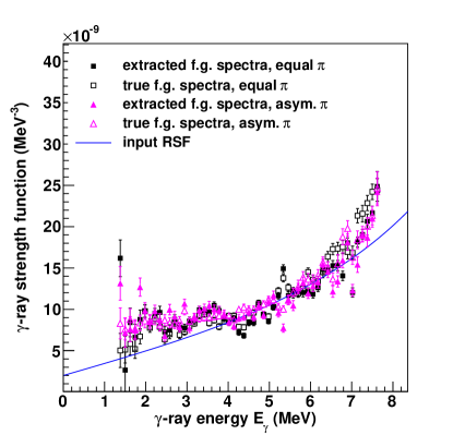
Figure 27: (Color online). Extracted strength functions from simulated data for an artificial ⁵⁷ Fe nucleus, with and without parity asymmetry in the level density.

Visually, it is hard to see any difference between the $\gamma$-ray strength functions with and without parity asymmetry. By taking the average $\gamma$-ray strength function for $\gamma$ energies between $1.4-3$ MeV, we find an average increase of about 20% for the case with parity asymmetry relative to the equal parity case, using the true first-generation spectra. The statistical fluctuations here are typically less than 10% for $E_{\gamma}=2-3$ MeV, and up to 40% for $\gamma$ rays below 2 MeV. If we use the extracted first-generation spectra from the folded data, the difference between the two cases is approximately 6–7%, less than the statistical fluctuations which are larger than when using the true first-generation spectra. For higher $E_{\gamma}$, there is no effect of parity within the fluctuations. We therefore conclude that it could be an effect of $\approx 20$% on the low-energy part of the $\gamma$-ray strength function. Hence, we find it reasonable to believe that even a considerable parity asymmetry on the level density as in the ⁵⁷Fe case will not drastically change the shape of the $\gamma$-ray strength function.

In Fig. 27, we note that there is an enhanced strength for $\gamma$-ray energies below $\approx 3.5$ MeV compared to the input $\gamma$-ray strength function, regardless of the parity distribution. This is in fact due to the spin range of the initial levels, which is further investigated in the following section.

III.5 The spin distribution

The uncertainty in the spin distribution may lead to errors in the Oslo method in three ways: (i) the extraction of first-generation $\gamma$ rays and subsequent effects on the extracted level density and $\gamma$-ray strength function, (ii) the estimation of $\rho(S_{n})$, and (iii) the spin range accessed experimentally (typically $0-8\hbar$ depending on the reaction and target spin) compared to the true, total spin distribution. These issues will be discussed in the following.

We have once more relied on simulated data applying the DICEBOX code DICEBOX in order to test the sensitivity on the final results with respect to the spin range of the initial levels. We simulated again a light nucleus that resembles ⁵⁷Fe, as we expect that light nuclei would be most sensitive to the initial spin population. This is because the higher spin levels are missing at low excitations. Again, the critical energy was set to 2.2 MeV, as there are no available data in the literature about levels with higher spins above this energy. As before, all levels had the same probability of population. The input $\gamma$-ray strength function model was independent of excitation energy.

Three spin ranges were used: $1/2\leq J\leq 7/2$, $1/2\leq J\leq 13/2$, and $7/2\leq J\leq 13/2$. This means that the highest possible spin reached at the final excitation energy was $9/2$ or $15/2$ depending on the maximum allowed initial spin. The weighting of the allowed spins followed the spin distribution of the input level density, which in this case was from the microscopic calculations of Ref. go08 . For all initial spin ranges we applied the full Oslo method, and in parallel we extracted the level density and $\gamma$-ray strength function from the true first-generation spectra. The resulting level densities and $\gamma$-ray strength functions are displayed in Figs. 28 and 29, respectively.

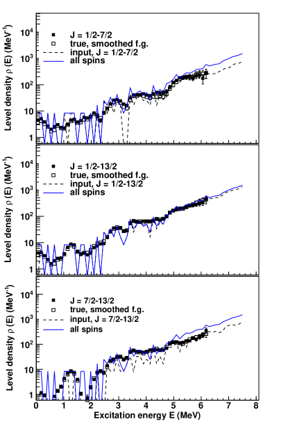
Figure 28: (Color online). Extracted level densities from simulated data for initial spin range $1/2\leq J\leq 7/2$ (top panel), $1/2\leq J\leq 13/2$ (middle panel), and $7/2\leq J\leq 13/2$ (bottom panel) on the initial levels.

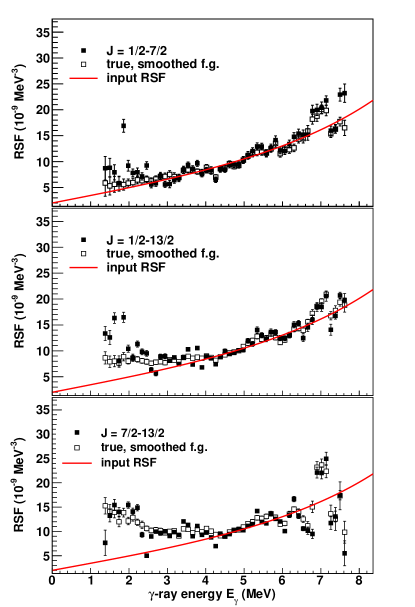
Figure 29: (Color online). Extracted strength functions for spin range $1/2\leq J\leq 7/2$ (top), $1/2\leq J\leq 13/2$ (middle), and $7/2\leq J\leq 13/2$ (bottom) on the initial levels.

As can be seen from Fig. 29, there is an enhanced strength at low $\gamma$ energies for the spin windows including the highest spins. Also, by looking at the average multiplicity $\langle M\rangle$ at 7.0 MeV of excitation energy, we get 1.8 for $1/2\leq J\leq 7/2$, 2.2 for $1/2\leq J\leq 13/2$, and 2.5 for $7/2\leq J\leq 13/2$. At $E_{\gamma}=2.1$ MeV, we find that the $\gamma$-ray strength function is increased with a factor of $\approx 1.7$ for the spin range $1/2\leq J\leq 13/2$, and a factor of $\approx 2.6$ for the spin range $7/2\leq J\leq 13/2$ with respect to the input $\gamma$-ray strength function. This is not an artifact from the unfolding or first-generation method, as it is also seen in the extracted $\gamma$-ray strength functions from the true first-generation spectra.

The explanation for the observed behavior is probably connected to three issues: (i) the dominance of dipole radiation, which carries $L=1$; (ii) the applied spin restriction on the initial levels; (iii) the low level density in this mass region at low excitation energies, especially for high spins. Let us take, as an example, the population of a 13/2 level at high excitation energy. If it is to decay to a low-lying level, involving a high-energy $\gamma$ transition, a level with appropriate spin must be present at this excitation energy. This is not necessarily the case as there are only about $2-10$ levels per 120 keV for excitation energies below 4.7 MeV. Among these few levels, there are probably no high-spin levels at all. This leads to a higher average multiplicity and an enhanced probability for decaying with low-energy $\gamma$ rays.

From Fig. 29, it is clear that the enhancement in the extracted $\gamma$-ray strength function is not present in the input $\gamma$-ray strength function, but is an effect of the three factors mentioned above. This means that the simple factorization in Eq. (10) of the first-generation spectra is not able to reproduce the input $\gamma$-ray strength function. The extracted $\gamma$-ray strength function, which could be considered as an ”effective” $\gamma$-ray strength function, is however fully capable of reproducing the true primary $\gamma$-ray spectra, and it is seen from Fig. 28 that the extracted level density is very reasonable indeed.

However, it is not obvious whether the spin range of the inital states is the full explanation of the observed low-energy enhancement in light and medium-mass nuclei. Further investigations are therefore needed to clarify this issue. It should also be noted that similar tests have been performed for an artificial nucleus resembling ¹⁶³Dy. No such enhancement was seen in this case, in agreement with experimental findings in this mass region. This is not surprising since in these nuclei, the level density is much higher and relatively high spins are available already at low excitation energies.

The quantity $\rho(S_{n})$ is calculated assuming a bell-like spin distribution according to Ref. GC given by Eq. (27) and using a model for the spin cutoff parameter $\sigma$ usually taken from Ref. GC or from Ref. egidy2 . Both these assumptions could in principle be a source of uncertainty, as it is hard or even impossible to measure experimentally the total spin distribution at high excitation energy. Thus, the theoretical spin distributions are seldom constrained to data for excitation energies higher than typically $2-3$ MeV.

In Fig. 30 various spin distributions for ⁴⁴Sc are shown, calculated at an excitation energy of 8.0 MeV. In the two upper panels, the spin distribution given in Eq. (27) has been used, but with the expression for the spin cutoff parameter of Refs. GC ; egidy1 in panel a) and the formalism of Ref. egidy2 in panel b). In panel c) the spin distribution of the spin-dependent level densities of Ref. Goriely1 are shown. Here, the authors also have assumed a bell-shaped spin distribution according to Eqs. (7) and (8) in Ref. Goriely1 . It is clear from the figure that the spin distributions in panel b) and c) are broader with centroids shifted to higher spins compared to the one in panel a).

In panel d), the spin distribution of the calculated spin- and parity-dependent level density of Ref. Goriely2 is shown. There are no underlying assumptions for the spin distribution in these calculations. It is seen from this distribution that there is a significant difference in the relative numbers of states with spin 0 and 1. The normalization procedure for the level density described above is especially sensitive to such variations at low spin if the neutron resonance spacing $D_{0}$ is measured from a neutron capture reaction where the target nucleus is even-even, that is, with zero ground-state spin. Then the states reached in neutron capture can only have spin $1/2^{+}$, and the number of all other states must be estimated using a certain spin cutoff parameter, introducing a larger uncertainty in the calculated $\rho(S_{n})$. Therefore it is preferred to calculate $\rho(S_{n})$ from both $D_{0}$ and $D_{1}$ resonance spacings if possible, since in the latter, also states with $3/2^{-}$ are reached for target nuclei with $I_{t}^{\pi}=0^{+}$, and will therefore decrease this uncertainty.

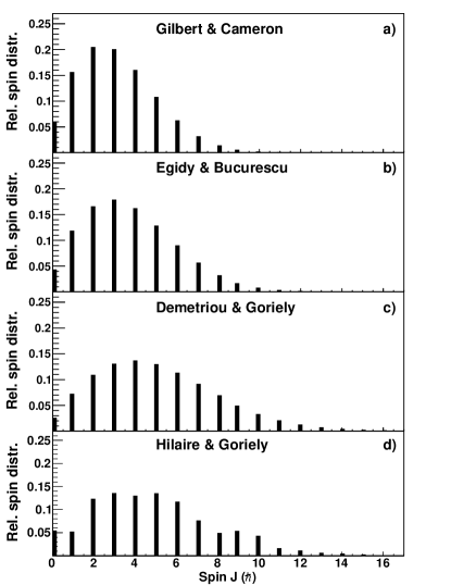
Figure 30: Relative spin distributions calculated for $E=8.0$ MeV of ⁴⁴Sc (see text).

We have investigated the relative difference in the value of $\rho(S_{n})$ for several nuclei using the spin-cutoff parameter of GC with global parameterization of egidy1 (referred to as Gilbert & Cameron), and the prescription of egidy2 (hereafter called von Egidy & Bucurescu), see Tab. 1. For the cases investigated here, the general trend is that the Gilbert & Cameron approach leads to a lower value for $\rho(S_{n})$ than the von Egidy & Bucurescu parameterization. However, this depends on the spins reached in the $(n,\gamma)$ reaction. For example, for ⁵¹V, we note that the obtained $\rho(S_{n})$ using the spin cutoff of von Egidy & Bucurescu is lower than that of Gilbert & Cameron. This is easily understood from the fact that in this case, relatively high spins are populated in the ($n,\gamma$) reaction. We see from Fig. 31 that the Gilbert & Cameron parameterization gives lower relative values for states with spin 11/2 and 13/2 compared to the von Egidy & Bucurescu distribution. Thus, one divides by a smaller number in Eq. (20) and $\rho(S_{n})$ gets larger.

Table 1: Variation of the calculated $\rho(S_{n})$ using different spin cutoff parameters. The target spin in the $(n,\gamma)$ reaction is denoted by $I_{t}^{\pi}$, and $E_{1}$ is the total backshift for the back-shifted Fermi-gas model while $a$ is the level-density parameter. All level spacings ($D_{0}$) are taken from RIPL . The parameter $\eta$ is the ratio $\rho_{EB}(S_{n})/\rho_{GC}(S_{n})$.

				Gilbert & Cameron				von Egidy & Bucurescu
Nucleus	$I_{t}^{\pi}$	$S_{n}$	$D_{0}$	$a$	$E_{1}$	$\sigma$	$\rho_{GC}(Sn)$	$a$	$E_{1}$	$\sigma$	$\rho_{EB}(Sn)$	$\eta$
		(MeV)	(keV)	(MeV-1)	(MeV)		(MeV-1)	(MeV-1)	(MeV)		(MeV-1)
51V	6+	11.05	2.3(6)	6.42	$-0.511$	3.24	$5.18\times 10^{3}$	6.17	$-0.153$	3.83	$4.15\times 10^{3}$	0.80
57Fe	0+	7.646	25.4(22)	7.08	$-0.910$	3.20	$8.46\times 10^{2}$	6.58	$-0.523$	3.83	$1.20\times 10^{3}$	1.41
96Mo	5/2+	9.154	0.105(10)	11.14	1.016	4.21	$7.38\times 10^{4}$	11.39	0.779	5.15	$1.01\times 10^{5}$	1.37
117Sn	0+	6.944	0.380(130)	13.23	0.197	4.48	$1.08\times 10^{5}$	13.62	$-0.210$	5.58	$1.67\times 10^{5}$	1.54
164Dy	5/2+	7.658	0.0068(6)	17.75	0.416	5.49	$1.74\times 10^{6}$	18.12	0.310	6.91	$2.59\times 10^{6}$	1.49

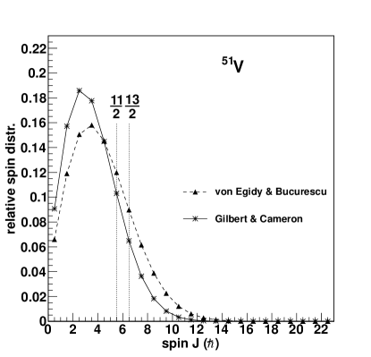
Figure 31: Relative spin distributions calculated at $S_{n}=11.051$ MeV of ⁵¹V (see text).

One can conclude that the two approaches studied here give a $\approx 10-50$% change in the resulting $\rho(S_{n})$, while other calculations go08 indicate even larger variations. Using this HFB-plus-combinatorial approach gives typically a factor of two change compared to $\rho_{GC}(S_{n})$ for most cases and up to a factor of 3.7 for the extreme case of ¹⁷²Dy (see Tab. II in Ref. go08 ). The effect of these differences is of course an uncertain determination of $\rho(S_{n})$ and thus of the slope of the level density and the $\gamma$-ray strength function, in a similar fashion as for the parity dependence (see Sec. III.4 and Fig. 26).

There is also a question of how the spin range accessed experimentally relative to the true, total spin range might influence structures in the level density. In the analysis, we assume that the excluded spins contribute on average with a scaling factor of the level density, which is corrected for by normalizing to $\rho(S_{n})$, i.e. the total level density for all spins at this energy. However, this relies on the hypothesis that structures in the level density due to, e.g., nucleon pair breaking are not severely affected by the spin window.

To test this, we have performed simplistic calculations with the code COMBI Ti45 , which is based on a microscopic, combinatorial model using Nilsson single-particle energies and the concept of quasiparticles from the nuclear Bardeen-Cooper-Schrieffer (BCS) theory. The chosen spin windows were $0\leq J\leq 6$ and $0\leq J\leq 30$ (in units of $\hbar$). Details of the model can be found in Ref. Ti45 .

The resulting calculated level densities for ⁵⁶Fe and ¹⁶⁴Dy are displayed in Figs. 32 and 33, respectively.

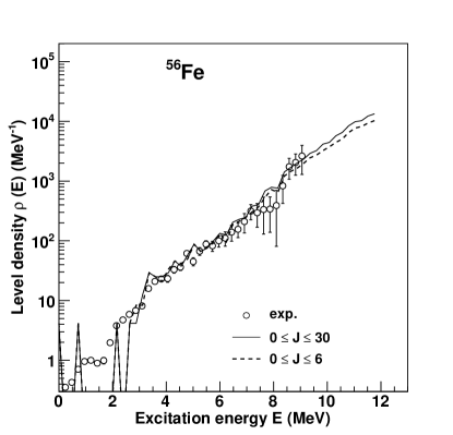
Figure 32: Calculated level density of ⁵⁶Fe for two spin ranges: $0\leq J\leq 6$ (dashed line) and $0\leq J\leq 30$ (solid line) compared to experimental data (open circles, from Ref. Fe_Emel ) normalized to the total level density at $S_{n}$.

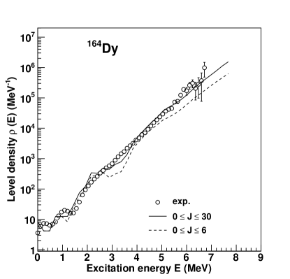
Figure 33: Same as Fig. 32 for ¹⁶⁴Dy, with experimental data from Ref. hildes_DyRSF .

For ⁵⁶Fe, is it clear that most of the states are found within the spin range of $0-6\hbar$. In fact, the relative difference between the large and the small spin window is at most $\approx 30$%, and it is clear that there are no significant structural differences for the two cases. One would therefore not expect any severe problems with normalizing the level density of such light nuclei to the total level density $\rho(S_{n})$. However, for the ¹⁶⁴Dy case, the deviation of the level densities calculated within the two spin ranges can be considerable and is increasing with excitation energy, up to a factor of $\approx 2.5$ for $E\approx 7.5$ MeV. It is nevertheless very gratifying that, indeed, the gross structures of the level densities are very much alike, so that extracted information from the experimental level density, such as the onset of the pair-breaking process, is probably reliable (the larger spin window leads to a smoothing of the steps). However, experimental work to investigate the spin distribution further is highly desirable.

IV Summary and conclusions

In this work we have addressed uncertainties and possible systematic errors that one can encounter using the Oslo method. The main steps of the method have been outlined, and the assumptions behind each step are investigated in detail. Our findings indicate that although the Oslo method is in general very robust, the various assumptions it relies on must be carefully considered when it is applied in different mass regions. The results can be summarized as follows.

The unfolding procedure. We have investigated the effect of changing the total absorption efficiencies of the NaI(Tl) crystals up to $\approx 20$%. We found that the extracted level density is hardly affected at all, while the $\gamma$-ray strength function gets a somewhat different slope. The quantitative effect on the $\gamma$-ray strength function corresponds directly to the imposed changes in the efficiencies.

The first-generation method. In general, the assumption of thermalization can be questioned at excitation energies above $\approx 10$ MeV. Also, variation in the populated spin range as a function of excitation energy may lead to an erroneous subtraction, especially of yrast states and other strong transitions at low $\gamma$-ray energies. This is particularly pronounced at low excitation and low $\gamma$-ray energies, where the direct reaction may favor or suppress the population of some levels compared to feeding from $\gamma$ decay. In addition, the finite, and for some energies, the mismatch of the detector resolution of the particle telescopes and CACTUS might in principle lead to problems with determining correct weighting functions. However, tests on simulated spectra show that this effect is probably of minor importance. The two different normalization options in the method turn out to give very similar results.

The Brink hypothesis. Since the extraction of level density and $\gamma$-ray strength relies on the Brink hypothesis, one would expect problems if there was an effective temperature dependence in the $\gamma$-ray strength function. From the results of simulated data, it is clear that especially the region of low $E_{\gamma}$ is affected when the $\gamma$-ray strength function is temperature dependent, and the extracted strength is found to found to lie in between the two temperature extremes considered. However, we note that there is, so far, no experimental evidence for any strong temperature dependence of the $\gamma$-ray strength function in the excitation-energy region in question (below $\approx 10$ MeV).

The parity distribution. The assumption of equally many positive- and negative-parity states may break down, especially for light nuclei, and would then affect the normalization of both the level density and the $\gamma$-ray strength function. If the parity asymmetry is large, the value of the normalization point $\rho(S_{n})$ might change with a factor of $\approx 2$, which will consequently change the slope of the level density and $\gamma$-ray strength function. For heavier nuclei, however, the parity distribution at $S_{n}$ is expected to be quite even, and experimental data on lighter nuclei suggest that the parity asymmetry should be small also here. Therefore, we find it reasonable to believe that the error in $\rho(S_{n})$ and on the absolute normalization of the $\gamma$-ray strength function due to this assumption does not exceed $50$%.

Another issue is the influence on the relative contribution of $E1$ and $M1$ transitions, as a large parity asymmetry will favor $M1$ transitions. Tests with simulated data indicate, however, that the effect is not large even with a considerable parity asymmetry.

The spin distribution. From simulations on light nuclei with different spin ranges on the initial levels, it is seen that the ranges including higher spins might lead to an enhanced $\gamma$-ray strength function at low $\gamma$-ray energies. This is understood from considering the relatively low level density and the matching of spins between the initial and final levels for dipole radiation. This could explain, at least partially, the observed enhanced low-energy strength in experimental data for light and medium-mass nuclei.

The spin distribution is one of the largest uncertainties in the normalization, since the determination of the slope of the level density and $\gamma$-ray strength function strongly depends on the relative intensities of the populated spins at $S_{n}$. Assuming a bell-shaped spin distribution with various global parameterizations of the spin cutoff parameter give up to $\approx 50$% change in $\rho(S_{n})$; however, microscopic calculations indicate that this value can vary within a factor of 2 or more, especially for nuclei in the rare-earth region. This will also consequently influence the $\gamma$-ray strength function.

The experimentally reached spin window in OCL experiments is typically $0-8\hbar$, which means that the extracted level-density data in fact represent this narrow spin range. This is usually compensated for by normalizing to the total level density at $S_{n}$. This is not a big effect for light nuclei with relatively few high-spin states. Even in the case of rare-earth nuclei, our calculations indicate that this scaling works well as the main structures in the level density are indeed present in the levels of a rather narrow spin range.

V Acknowledgments

The authors wish to thank E. A. Olsen and J. Wikne for providing excellent experimental conditions. Financial support from the Research Council of Norway (NFR), project no. 180663, is gratefully acknowledged.

References

- (1) J. Rekstad et. al., Physica Scripta Vol. T5, 45 (1983).
- (2) A. Schiller, A. Voinov, E. Algin, J. A. Becker, L. A. Bernstein, P. E. Garrett, M. Guttormsen, R. O. Nelson, J. Rekstad, and S. Siem, Phys. Lett. B 633 225 (2006).
- (3) U. Agvaanluvsan, A. Schiller, J. A. Becker, L. A. Bernstein, P. E. Garrett, M. Guttormsen, G. E. Mitchell, J. Rekstad, S. Siem, A. Voinov, and W. Younes, Phys. Rev. C 70, 054611 (2004).
- (4) M. Guttormsen, A. Bagheri, R. Chankova, J. Rekstad, A. Schiller, S. Siem, and A. Voinov, Phys. Rev. C 68, 064306 (2003).
- (5) H. T. Nyhus, S. Siem, M. Guttormsen, A. C. Larsen, A. Bürger, N. U. H. Syed, G. M. Tveten, and A. Voinov, Phys. Rev. C 81, 024325 (2010).
- (6) E. Melby, L. Bergholt, M. Guttormsen, M. Hjorth-Jensen, F. Ingebretsen, S. Messelt, J. Rekstad, A. Schiller, S. Siem, and S. W. Ødegård, Phys. Rev. Lett. 83, 3150 (1999).
- (7) U. Agvaanluvsan, A. C. Larsen, M. Guttormsen, R. Chankova, G. E. Mitchell, A. Schiller, S. Siem, and A. Voinov, Phys. Rev. C 79, 014320 (2009).
- (8) U. Agvaanluvsan, A. C. Larsen, R. Chankova, M. Guttormsen, G. E. Mitchell, A. Schiller, S. Siem, and A. Voinov, Phys. Rev. Lett. 102, 162504 (2009).
- (9) H. K. Toft, A. C. Larsen, U. Agvaanluvsan, A. Bürger, M. Guttormsen, G. E. Mitchell, H. T. Nyhus, A. Schiller, S. Siem, N. U. H. Syed, and A. Voinov, Phys. Rev. C 81, 064311 (2010).
- (10) A. Voinov, E. Algin, U. Agvaanluvsan, T. Belgya, R. Chankova, M. Guttormsen, G.E. Mitchell, J. Rekstad, A. Schiller, and S. Siem, Phys. Rev. Lett 93, 142504 (2004).
- (11) E. Algin, U. Agvaanluvsan, M. Guttormsen, A. C. Larsen, G. E. Mitchell, J. Rekstad, A. Schiller, S. Siem, and A. Voinov, Phys. Rev. C 78, 054321 (2008).
- (12) M. Guttormsen, R. Chankova, U. Agvaanluvsan, E. Algin, L.A. Bernstein, F. Ingebretsen, T. Lönnroth, S. Messelt, G.E. Mitchell, J. Rekstad, A. Schiller, S. Siem, A. C. Sunde, A. Voinov and S. Ødegård, Phys. Rev. C 71, 044307 (2005).
- (13) A. C. Larsen, R. Chankova, M. Guttormsen, F. Ingebretsen, T. Lönnroth, S. Messelt, J. Rekstad, A. Schiller, S. Siem, N. U. H. Syed, A. Voinov, and S. W. Ødegård, Phys. Rev. C 73, 064301 (2006).
- (14) A. C. Larsen, M. Guttormsen, R. Chankova, F. Ingebretsen, T. Lönnroth, S. Messelt, J. Rekstad, A. Schiller, S. Siem, N. U. H. Syed, and A. Voinov, Phys. Rev. C 76, 044303 (2007).
- (15) M. Guttormsen, A. C. Larsen, A. Bürger, A. Görgen, S. Harissopulos, M. Kmiecik, T. Konstantinopoulos, M. Krtic̆ka, A. Lagoyannis, T. Lönnroth, K. Mazurek, M. Norrby, H. T. Nyhus, G. Perdikakis, A. Schiller, S. Siem, A. Spyrou, N. U. H. Syed, H. K. Toft, G. M. Tveten, and A. Voinov, Phys. Rev. C 83, 014312 (2011).
- (16) A. C. Larsen and S. Goriely, Phys. Rev. C 82, 014318 (2010).
- (17) M. Guttormsen, A. Ataç, G. Løvhøiden, S. Messelt, T. Ramsøy, J. Rekstad, T.F. Thorsteinsen, T.S. Tveter, and Z. Zelazny, Phys. Scr. T 32, 54 (1990).
- (18) M. Guttormsen, T. S. Tveter, L. Bergholt, F. Ingebretsen, and J. Rekstad, Nucl. Instrum. Methods Phys. Res. A 374, 371 (1996).
- (19) M. Guttormsen, T. Ramsøy, and J. Rekstad, Nucl. Instrum. Methods Phys. Res. A 255, 518 (1987).
- (20) G. A. Bartholomew, I. Bergqvist, E. D. Earle, and A. J. Ferguson, Can. J. Phys. 48, 687 (1970).
- (21) J. Rekstad, A. Henriquez, F. Ingebretsen, G. Midttun, B. Skaali, R. Øyan, J. Wikne, and T. Engeland, Phys. Scr. T 5, 45 (1983).
- (22) A. Bohr and B. Mottelson, Nuclear Structure, Benjamin, New York, 1969, Vol. I.
- (23) L. Henden, L. Bergholt, M. Guttormsen, J. Rekstad, and T. S. Tveter, Nucl. Phys. A589, 249 (1995).
- (24) D. M. Brink, Ph.D. thesis, p.101-110, Oxford University, 1955.
- (25) A. Schiller, L. Bergholt, M. Guttormsen, E. Melby, J. Rekstad, and S. Siem, Nucl. Instrum. Methods Phys. Res. A 447, 498 (2000).
- (26) C. E. Porter and R. G. Thomas, Phys. Rev. 104, 483 (1956).
- (27) A. Gilbert and A. G. W. Cameron, Can. J. Phys. 43, 1446 (1965).
- (28) T. von Egidy, H. H. Schmidt and A. N. Behkami, Nucl. Phys. A 481 (1988) 189.
- (29) T. von Egidy and D. Bucurescu, Phys. Rev. C 72, 044311 (2005); Phys. Rev. C 73, 049901(E) (2006).
- (30) N. U. H. Syed, M. Guttormsen, F. Ingebretsen, A. C. Larsen, T. Lönnroth, J. Rekstad, A. Schiller, S. Siem, and A. Voinov, Phys. Rev. C 79, 024316 (2009).
- (31) A. Voinov, M. Guttormsen, E. Melby, J. Rekstad, A. Schiller, and S. Siem, Phys. Rev. C 63, 044313 (2001).
- (32) J. Kopecky and M. Uhl, Phys. Rev. C41, 1941 (1990).
- (33) T. Belgya, O. Bersillon, R. Capote, T. Fukahori, G. Zhigang, S. Goriely, M. Herman, A. V. Ignatyuk, S. Kailas, A. Koning, P. Oblozinsky, V. Plujko and P. Young, Handbook for calculations of nuclear reaction data, RIPL-2. IAEA-TECDOC-1506 (IAEA, Vienna, 2006).
- (34) F. Bec̆vár̆, Nucl. Instrum. Methods Phys. Res. A 417, 434 (1998).
- (35) E. Běták, in Proceedings of the Second International Workshop on Compond Nuclear Reactions and Related Topics, 58 October 2009, Bordeaux, France, EPJ Web of Conferences 2, 11002 (2010).
- (36) J. W. Smith, L. Meyer-Schützmeister, T. H. Braid, P. P. Singh, and G. Hardie, Phys. Rev. C 7, 1099 (1973).
- (37) A. Schiller and M. Thoennessen, At. Data Nucl. Data Tables 93, 549 (2007).
- (38) U. Agvaanluvsan, G. E. Mitchell, J. F. Shriner Jr., and M. Pato, Phys. Rev. C 67, 064608 (2003).
- (39) S. Goriely, S. Hilaire, and A. J. Koning, Phys. Rev. C 78, 064307 (2008).
- (40) Y. Alhassid, G. F. Bertsch, S. Liu, and H. Nakada, Phys. Rev. Lett 84, 4313 (2000).
- (41) D. Mocelj, T. Rauscher, G. Martínez-Pinedo, K. Langanke, L. Pacearescu, A. Faessler, F.-K. Thielemann, and Y. Alhassid, Phys. Rev. C 75, 045805 (2007).
- (42) Y. Kalmykov, C. Özen, K. Langanke, G. Martínez-Pinedo, P. von Neumann-Cosel, and A. Richter, Phys. Rev. Lett 99, 202502 (2007).
- (43) S. G. Kadmenskiĭ, V. P. Markushev, and V. I. Furman, Sov. J. Nucl. Phys. 37, 165 (1983).
- (44) P. Demetriou and S. Goriely, Nucl. Phys. A 695, 95 (2001).
- (45) S. Hilaire and S. Goriely, Nucl. Phys. A 779, 63 (2006).
- (46) N. U. H. Syed, A. C. Larsen, A. Bürger, M. Guttormsen, S. Harissopulos, M. Kmiecik, T. Konstantinopoulos, M. Krtic̆ka, A. Lagoyannis, T. Lönnroth, K. Mazurek, M. Norrby, H. T. Nyhus, G. Perdikakis, S. Siem, and A. Spyrou, Phys. Rev. C 80, 044309 (2009).