Modelling the Polarisation of Microwave Foreground Emission on Large Angular Scales

Abstract

Templates for polarised emission from Galactic foregrounds at frequencies relevant to Cosmic Microwave Background (CMB) polarisation experiments are obtained by modelling the Galactic Magnetic Field (GMF) on large scales. This work extends the results of O’Dea et al. (2012) (hereafter FGPolI) by including polarised synchrotron radiation as a source of foreground emission. The polarisation direction and fraction in this calculation are based solely on the underlying choice of GMF model and therefore provide an independent prediction for the polarisation signal on large scales. Templates of polarised foregrounds may be of use when forecasting effective experimental sensitivity. In turn, as measurements of the CMB polarisation over large fractions of the sky become routine, this model will allow for the data to constrain parameters in the, as yet, not well understood form of the GMF. Template foreground maps at a range of frequencies can be downloaded from the on-line repository .

1 Introduction

Currently operating or upcoming CMB experiments such as EBEX (Reichborn-Kjennerud et al., 2010), Spider (Filippini et al., 2010), POLARBEAR (The Polarbear Collaboration et al., 2010), Keck (Sheehy et al., 2011) and ABS (Essinger-Hileman et al., 2010) will routinely reach the sensitivity in polarisation required to detect the curl-type pattern ($B$-mode) predicted by the simplest models of inflation (Dodelson et al., 2009). The predicted amplitude of this signal however is comparable or below the predicted signal of foreground polarisation over all observationally relevant frequencies and over most of the sky (Gold et al., 2011). For polarisation in particular the foreground signal is dominated by synchrotron emission at low frequencies ($\lesssim$ 100 GHz) and thermal dust emission at high frequencies ($\gtrsim$ 100 GHz).

Given the high levels of polarised foregrounds the mission planning for these and future experiments requires a detailed study of sky coverage to optimise sensitivity to the $B$-mode signal. The impact of the trade off between larger sky coverage, depth of observation and the ‘cleanliness’ of or lack of Galactic foregrounds in a patch of sky must all be considered. Regardless of how clean the final observed sky patch, some level of foreground removal will be required for all experiments. Realistic foreground templates based on models and/or observations of the polarisation direction and amplitude of foregrounds are very useful when carrying out this work. However, reliable templates of polarised foregrounds at the frequencies relevant to CMB observations have been hard to come by and only recently, with Wilkinson Microwave Anisotropy Probe (WMAP) $K$-band observations have reliable estimates of synchrotron polarisation on large angular scales been made.

Little other polarization data exists at the frequencies of interest for future CMB experiments (with frequency bands ranging from $90$ GHz up to $450$ GHz), hence it is necessary to model foreground emission by extrapolating the information from existing data. This paper builds on previous work presented in FGPolI, which described a model for foreground emission due to interstellar dust in the Galaxy. The dust model was introduced by O’Dea (2009) and first applied in O’Dea et al. (2011) for the purpose of studying the impact of polarised foreground dust on Spider’s ability to detect $B$-mode polarisation. FGPolI gives a detailed explanation of the dust model and presents a number of full-sky template maps at various frequencies. A complete model of polarised foreground emission must also include the effect of synchrotron emission. This is particularly important for low frequency observations i.e. below the CMB ‘sweet-spot’ at 100 GHz. This will be the focus of the work reported here. Additional components due to spinning dust and free-free emission are not thought to give a significant signal in polarisation and are omitted in our modelling (see for example Macellari et al. (2011) and López-Caraballo et al. (2011)).

Synchrotron emission, generated by the gyration of cosmic ray electrons in the Galactic magnetic field (GMF), is intrinsically polarised and constitutes the main polarised foreground at lower frequencies (Page et al., 2007). While the emission from thermal dust is expected to be higher than synchrotron emission above around $90$ GHz, the signal from synchrotron is also not negligible. With the addition of synchrotron, this paper provides a complete model of polarised microwave foreground emission on large angular scales. Here a detailed explanation of the synchrotron model is given and full-sky template maps are presented. As with previous work the model includes a three dimensional description of the Galactic magnetic field on both large and small spatial scales. Both polarisation amplitude and angle are modelled internally and the templates are scaled such that the polarisation amplitude corresponds to a nominal value when averaged over the maps.

This paper is organized as follows. Section 2 briefly reviews the mechanism for synchrotron emission. Section 3 describes the synchrotron model including the underlying GMF, the choice of total intensity template, and the cosmic ray density distribution and line-of-sight integration method required to evaluate the final Stokes parameters maps. In Section 4 examples of template maps produced using this model are described and in Section 5 the templates are are compared with the WMAP estimated foreground maps. Section 6 compares the level of foreground polarisation in the templates in coverage areas of a sample of currently planned or operating sub-orbital experiments. We conclude with some discussion in Section 7.

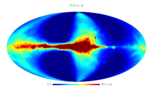
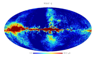
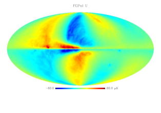
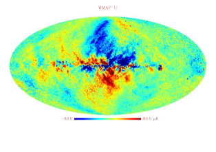
Figure 1: From top to bottom, $Q$ and $U$ Stokes parameter template maps, displayed in Galactic co-ordinates for left: FGPol model of synchrotron emission at $23$ GHz for the LSA GMF model. These were generated at $N_{\rm side}=1024$ map resolution based on $N_{\rm side}^{\rm P}=128$ line-of-sight resolution. The maps are smoothed to $1^{\circ}$ and downgraded to $N_{\rm side}=64$. right: WMAP MCMC synchrotron map for comparison. Units are $\mu K$ antenna temperature.

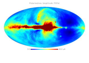
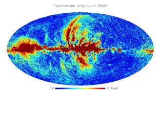
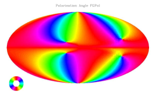
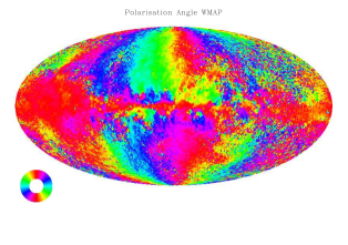
Figure 2: Polarisation amplitude ($P=\sqrt{Q^{2}+U^{2}}$) in antenna temperature ($\mu K$) (top) and angle (bottom) in Galactic co-ordinates for the synchrotron emission template (LSA GMF model) at 23 GHz (left) and for WMAP 23GHz (right). The polarisation angle colour coding ranges from 0 to 180 degrees.

2 Polarised Synchrotron Emission

Diffuse synchrotron emission is one of the dominant Galactic foregrounds for CMB observations. The synchrotron radiation arises when electrons with large relativistic energies are accelerated in the GMF. The frequency dependence of synchrotron emission depends on the energy spectrum of these cosmic-ray electrons, as well as the intensity of the GMF (see e.g.  Rybicki & Lightman (1979)). An ensemble of relativistic electrons with a power law distribution in energy produces a synchrotron emission spectrum that is another power law ( Longair (1994)). At GeV energies, where radio synchrotron emission peaks, the index of the power law is expected to have a range between $\beta\sim-3.5\rightarrow-2.5$ (Rybicki & Lightman, 1979) in inferred antenna temperature or, equivalently, $\alpha\sim-1.5\rightarrow-0.5$ in specific intensity. Since the spectral index has been seen to vary with position across the sky (Hinshaw et al., 2007), such a power law in antenna temperature describing synchrotron emission is only an approximation. In addition, the highest energy electrons lose energy more quickly resulting in a gradual steepening in the power law index at the higher frequencies (Bennett et al., 2003).

At microwave frequencies polarised foreground emission is dominated by polarised synchrotron and thermal dust that are both sensitive to the coherent GMF (Page et al., 2007). The dominant emission at lower frequencies is polarised synchrotron radiation. WMAP measurements from its lower frequency bands provide important constraints on polarised synchrotron emission. Synchrotron emission is linearly polarised with direction perpendicular to the projection of the GMF on the plane of the sky (see for example Rybicki & Lightman (1979)). The degree of synchrotron polarisation depends greatly on position on the sky and observing frequency. Changes in magnetic field direction along the line-of-sight leads to a depolarization effect, reducing the fractional polarisation degree of synchrotron emission. At frequencies lower than $\sim$ 1 GHz, depolarization is significant and hence synchrotron polarisation is as low as few tens of percent (Spoelstra, 1984). At CMB frequencies, depolarisation is minimal, with the degree of synchrotron polarisation being as high as 30 to 50 % in some galactic structure.

Free-free emission and spinning dust are also thought to contribute to the foreground signal in total intensity over a range of frequencies. For example, anomalous microwave emission around 20GHz has been found in WMAP data, with suggestions that this is more likely due to spinning dust emission than a flat synchrotron component (Peel et al., 2011). However spinning dust and free-free emission are not thought to be significantly polarised and their impact on final estimates of e.g. the tensor-to-scalar ratio $r$ is minimal (Armitage-Caplan et al., 2012) at about the 1% level.

Aside from the spatial dependence of the polarisation angle and amplitude, significant uncertainties remain in the frequency modelling of synchrotron intensity. For example, Bennett et al. (2003) argue that at higher Galactic latitudes (in the halo) the spectral index $\beta\sim-3$ while in the Galactic plane (near star forming regions) $\beta\sim-2.5$. This results in differences in the observed structure between WMAP $K$-band at 23GHz and the Haslam map at 408MHz (Haslam et al., 1982) as regions with flatter spectral index become more important at higher frequencies. However Miville-Deschenes et al. (2008) find a lower range of variation of the spectral index. This work focuses only on the polarisation fraction and orientation due to the assumed GMF model. We assume a simple frequency scaling of the Haslam template with a single spectral index multiplying the internally modelled polarisation fraction to provide morphologically realistic templates. A more detailed, possibly pixel dependent, frequency rescaling can always be introduced by rescaling the template obtained.

A number of other studies aimed at modelling foreground emission at microwave frequencies have been carried out (see e.g. Fauvet et al. (2010), Page et al. (2007)). An extensive study modelling different foregrounds in both intensity and polarisation over a large range in angular scales is the Planck Sky Model (PSM) (Delabrouille et al., 2012). It includes detailed modelling of Galactic diffuse emission, including synchrotron and thermal dust emission as well as free-free, spinning dust and CO lines. It also includes information on Galactic HII regions, extragalactic radio sources and several other sources of emission.

At present the best template of polarised Galactic synchrotron emission is that provided by the WMAP $K$-band (23GHz) whilst the intensity has been well measured (free from CMB contamination) at 408MHz by the Haslam all sky survey. As detailed below we use the Haslam maps to introduce detailed morphology in our templates since the WMAP Maximum Entropy Method (MEM) maps still contain a significant noise residual due to CMB contamination at the smoothing scale adopted (1^∘). We compare the templates obtained here with the WMAP synchrotron and dust maps obtained through their Monte Carlo Markov Chain (MCMC) best–fit procedure (Gold et al., 2011). Similar templates (Fauvet et al., 2010) have been compared with Archeops maps over a limited fraction of the sky at 353 GHz (Benoît et al., 2004) but these maps are not publicly available.

3 Model

3.1 Galactic Magnetic Field Model

A number of magnetic field models were compared in FGPolI . Here we limit the choice to the Logarithmic Spiral Arm (LSA) model introduced by Page et al. (2007) for use in modelling the WMAP data. The model is defined as

$$B_{\rho} =-B_{0}\sin{\left(\psi_{0}+\psi_{1}\ln{\frac{\rho}{\rho_{\rm W}}}\right)}\cos{\chi}\,,$$

$$B_{\Phi} =-B_{0}\cos{\left(\psi_{0}+\psi_{1}\ln{\frac{\rho}{\rho_{\rm W}}}\right)}\cos{\chi}\,,$$

$$B_{z} =B_{0}\sin{\chi}\,,$$ (1)

where $\rho$, $\Phi$ and $z$ are Galacto-centric cylindrical co-ordinates with $\Phi$, the cylindrical longitude, measured from the direction of the Sun, $\chi=\chi_{0}\tanh(z/z_{0})$ parametrizes the amplitude of the $z$ component and $z_{0}=1$ kpc. The field amplitude is set to $B_{0}=3\mu$G, and we take the distance between the Sun and the Galactic center to be $8$ kpc. Best-fit parameter values obtained by fits to the WMAP $K$-band field directions are $\psi_{0}=27$ degrees, $\psi_{1}=0.9$ degrees, and $\chi_{0}=25$ degrees. The radial scale is set to $\rho_{\rm W}=8$ kpc and the scale height is set to $z_{0}=1$ kpc.

Although we focus on large angular scales we also include a small-scale random component in our GMF model by adding a realisation of a Kolmogorov turbulence field with a one-dimensional Kolmogorov energy spectral index of $-5/3$. An injection scale of $100$ pc is chosen for the turbulent realisation with a negligibly small dissipation scale compared to the resolution scale.

3.2 Cosmic Ray Density Distribution

To model synchrotron emission a three-dimensional model of the distribution of cosmic rays in the Galaxy is required. The large-scale spatial distribution of the cosmic rays is modelled through its density, $n_{\rm cr}$, and is thought to follow the same form as the dust distribution with modified radial and scale heights (Page et al., 2007),

$$n_{\rm cr}=n_{0}\exp{\left(-\frac{\rho}{\rho_{{\rm cr}}}\right)}\mathrm{\,sech\,}^{2}{\left(\frac{z}{z_{{\rm cr}}}\right)}\,.$$ (2)

where the height and radial scales are set to $z_{{\rm cr}}=1$ kpc and $\rho_{{\rm cr}}=5$ kpc. These parameter values were chosen for the WMAP analysis of Page et al. (2007) following work by Drimmel & Spergel (2001).

3.3 Total Intensity

Our method aims to predict the polarisation amplitude and angle based on a chosen GMF model. The choice of total intensity for our templates is therefore external to the model and can be set to reflect any existing template. For synchrotron emission we chose to scale the point source corrected Haslam all-sky survey using a single power law in antenna temperature for simplicity. This scaled map is also multiplied by the internally modelled polarisation fraction template to produce Stokes parameter maps with realistic morphology.

The Haslam template in brightness temperature, with a resolution of $0.85^{\circ}$, is scaled to microwave frequencies using a spectral index $\beta_{s}=-3$. Although the map may contain residual contamination by free-free emission (see e.g. Dickinson, Davies & Davis (2003)) we assume it is dominated by the synchrotron component. The templates can be rescaled using any choice of templates in future.

3.4 Stokes Parameters

The direction and degree of polarisation from synchrotron emission are highly dependent on the Galactic magnetic field. To model these we integrate along lines-of-sight using the GMF outlined in section 3.1. The full-sky maps presented here were obtained using a one-dimensional realisation of the small-scale turbulent field. When producing smaller patches that require much fewer lines-of-sight at a given resolution we model the small scale turbulence as a full three-dimensional random realisation which preserves the spatial correlations implied by the Kolmogorov spectrum.

The total GMF model is made up of a sum of large-scale (ls) and small-scale (ss) components with

$$B_{r}=B_{r,\rm{ss}}+B_{r,{\rm ls}}\,,$$

$$B_{\theta}=B_{\theta,{\rm ss}}+B_{\theta,{\rm ls}}\,,$$

$$B_{\phi}=B_{\phi,{\rm ss}}+B_{\phi,{\rm ls}}\,,$$ (3)

where $r$, $\theta$, and $\phi$ are now Solar-centric spherical polar co-ordinates. The polarisation at each point along the line-of-sight $\hat{r}$ is determined by the perpendicular field components, $B_{\theta}$ and $B_{\phi}$.

The Stokes parameters for the synchrotron model are then projected out from the three-dimensional model using the appropriate line-of-sight integrals,

$$I_{\rm model}(\theta,\phi) =\epsilon(\nu)\int_{0}^{r_{\max}}n_{{\rm cr}}(\boldsymbol{r})(B_{\phi}(\boldsymbol{r})^{2}+B_{\theta}(\boldsymbol{r})^{2})\,{\mathrm{d}}r\,,$$

$$Q_{\rm model}(\theta,\phi) =\epsilon(\nu)\int_{0}^{r_{\max}}n_{{\rm cr}}(\boldsymbol{r})p\frac{(B_{\phi}(\boldsymbol{r})^{2}-B_{\theta}(\boldsymbol{r})^{2})B_{r}^{2}}{{B^{2}}}\,{\mathrm{d}}r\,,$$

$$U_{\rm model}(\theta,\phi) =\epsilon(\nu)\int_{0}^{r_{\max}}n_{{\rm cr}}(\boldsymbol{r})p\frac{2B_{\phi}(\boldsymbol{r})B_{\theta}(\boldsymbol{r})B_{r}^{2}}{{B^{2}}}\,{\mathrm{d}}r\,,$$ (4)

where $B^{2}=B_{r}^{2}+B_{\phi}^{2}+B_{\theta}^{2}$ and $\epsilon$ is the emissivity as a function of frequency, $\nu$. As with the dust templates, we conform to the default convention applied in the healpix package (Górski et al., 2005) regarding the sign of $U$.

Having computed the line-of-sight integrals for the Stokes parameters we calculate maps of the polarisation direction, $\gamma$, and degree, $P$, given by

$$P(\theta,\phi) =\frac{\sqrt{Q_{\rm model}^{2}+U_{\rm model}^{2}}}{I_{\rm model}}\,,$$

$$\gamma(\theta,\phi) =\frac{1}{2}\arctan{\left(\frac{U_{\rm model}}{Q_{\rm model}}\right)}\,.$$ (5)

The final synchrotron template at frequency $\nu$ is then obtained by scaling with the Haslam template

$$I^{\nu}_{{\rm sync}}(\theta,\phi) =I^{\nu}_{{\rm Has}}(\theta,\phi)\,,$$

$$Q^{\nu}_{{\rm sync}}(\theta,\phi) =I^{\nu}_{{\rm Has}}(\theta,\phi)\,P(\theta,\phi)\,\cos\left(2\,\gamma(\theta,\phi)\right)\,,$$

$$U^{\nu}_{{\rm sync}}(\theta,\phi) =I^{\nu}_{{\rm Has}}(\theta,\phi)\,P(\theta,\phi)\,\sin\left(2\,\gamma(\theta,\phi)\right)\,,$$ (6)

where $I_{{\rm Has}}^{\nu}$ is the total intensity of the Haslam map extrapolated to frequency $\nu$.

4 Maps

Figure 1 shows $Q$ and $U$ Stokes parameter maps at 23GHz for the whole sky arising from the model with their amplitudes scaled such that the polarisation amplitude corresponds to that of the WMAP counterpart (also shown) when averaged over the maps. The morphology of the polarisation agrees well with the observations with the most visible difference being on scales of a few degrees where the WMAP estimates are dominated by residual noise.

The resolution of the healpix maps is $N_{\rm side}=1024$ but the polarisation information is based on a line-of-sight integral at an angular resolution of $N_{\rm side}^{\rm P}=128$, corresponding to roughly $\ell\sim 500$ in multipole space. We integrate along lines-of-sight to the centre of all healpix pixels at a given $N_{\rm side}^{\rm P}$ from zero out to a maximum distance $r_{\max}$ of 30,000 pc, with discretisation steps of $0.1$ pc. $N_{\rm side}^{\rm P}$ is less than or equal to $N_{\rm side}$ of the total intensity Haslam map.

The LSA model is used for the Galactic magnetic field model with the same parameters as in FGPolI. The small scale field is modeled as Kolmogorov turbulence in 1D for large patches of sky, with a power spectrum of $\mathcal{P}(k)\propto k^{-(2+3\,N_{d})/3}$ where $N_{d}$ is the number of spatial dimensions of the realisation and $k$ is the magnitude of the wavevector. All full-sky templates presented here make use of the 1D approximation along the line-of-sight for the small scale turbulent component of the GMF. Small patch templates discussed below are produced with full 3D realisations of the field in the (smaller) volume probed by the reduced coverage.

Figure 2 shows maps of $P$ and $\gamma$ obtained using this choice of resolution and modelling of large and small scales. For comparison, maps of $P$ and $\gamma$ for the WMAP 23GHz MCMC template are also plotted. Differences between the templates and observations are mostly due to noise but there are also obvious differences in the morphology along the galactic plane and around the largest Galactic features such as the Galactic centre and North and South Galactic Spurs. Some of these differences are related to our choice of total intensity template which uses the Haslam maps at 408 MHz. A comparison between the scaled Haslam map and synchrotron templates obtain via the differencing of WMAP $K$ and $Ka$ bands were discussed in Gold et al. (2011). Below we quantitatively compare the broad features of both synchrotron and dust full–sky templates with the corresponding WMAP MCMC best–fit maps.

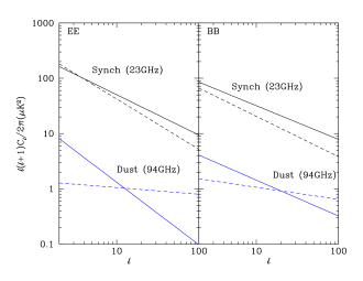
Figure 3: $EE$ (left) and $BB$ (right) fits to the foreground angular power spectra for the WMAP MCMC synchrotron 23GHz and dust 94GHz maps (solid line) compared to the FGPol synchrotron model and dust model (dashed line). The polarisation amplitude of the model templates is matched to the WMAP MCMC templates as described in the text. The fit values used are given in Table 1. These were calculated from maps masked with a union of the WMAP P06 mask and the MCMC flagged pixels.

Component	A [$\mu K^{2}$]	m
WMAP MCMC
Synchrotron $EE$	306 $\pm$ 95	$-0.91$ $\pm$ 0.11
Synchrotron $BB$	144 $\pm$ 44	$-0.87$ $\pm$ 0.12
Dust $EE$	12.9 $\pm$ 6.4	$-1.06$ $\pm$ 0.24
Dust $BB$	6.12 $\pm$ 3.7	$-0.83$ $\pm$ 0.29
FGPol
Synchrotron $EE$	343 $\pm$ 91	$-1.05$ $\pm$ 0.09
Synchrotron $BB$	110 $\pm$ 29	$-0.73$ $\pm$ 0.08
Dust $EE$	1.38 $\pm$ 0.33	$-0.12$ $\pm$ 0.07
Dust $BB$	1.70 $\pm$ 0.37	$-0.22$ $\pm$ 0.06

Table 1: Foreground power law + white noise fits of WMAP MCMC and FGPol template spectra outside the combination of P06 mask and MCMC flagged pixels. There is good agreement in both $EE$ and $BB$ for synchrotron between the FGPol template and the WMAP MCMC synchrotron component map. The FGPol dust template shows a significantly shallower spectrum than the WMAP MCMC component map indicating relatively more structure at large angular scales.

5 Comparison with WMAP templates

The WMAP satellite observations provide full–sky maps of temperature and polarisation in five frequency bands between 23GHz and 94GHz (Jarosik et al., 2011). The polarisation maps contain important information on Galactic foreground emission and hence provide an important test of our model of Galactic synchrotron radiation. Synchrotron radiation dominates the measured signal in the lower frequency bands, and we use the best fit WMAP 23GHz synchrotron templates generated by an MCMC fit for comparison with our model. Thermal dust emission dominates higher frequency bands, and for comparison with our dust model we use the 94GHz dust templates generated from the MCMC best fit values.

We use the WMAP MCMC ‘base’ fit which includes three power law foregrounds: dust, synchrotron and free-free emission as well as a contribution from CMB. These maps are smoothed at a scale of $1^{\circ}$ and have been downgraded to $N_{\rm side}=64$ before the MCMC fit is carried out. The WMAP team performed a combined MCMC fit to their five bands at a resolution of $N_{\rm side}=64$. The pixel noise is calculated at $N_{\rm side}=512$ and downgraded to $N_{\rm side}=64$.

FGPol templates are normalised to the polarisation amplitude $P=\sqrt{Q^{2}+U^{2}}$ of the full sky WMAP MCMC template with no masking or smoothing. The model maps are generated at $N_{\rm side}=1024$ for the large scale resolution and $N_{\rm side}^{\rm P}=128$ for the small scale line-of-sight resolution, then smoothed with a Gaussian beam of $1^{\circ}$ and degraded to $N_{\rm side}=64$.

Angular power spectra $C_{\ell}^{XX}$ for $XX\equiv TT,EE$, and $BB$ of both templates were calculated after masking with the P06 polarisation mask (Page et al., 2007) combined with a mask of pixels flagged by the WMAP MCMC process. The spectra are corrected for sky fraction $f_{\rm sky}$ effects and for their respective pixel and beam smoothing functions and then fit for a power law in multipole $\ell$ with an additional white noise component

$$\frac{\ell(\ell+1)}{2\pi}C_{\ell} =A\ell^{m}+\ell(\ell+1)N^{2}\,$$ (7)

where $A$ is the amplitude of the foreground component, $m$ is the index and $N$ is the noise amplitude. This procedure is similar to that carried out by Gold et al. (2011). Although the scatter at large angular scales is non-Gaussian and somewhat correlated by the sky cut we adopt a very simple assumption for sample variance in the power spectra by disregarding correlations between multipoles and assuming a Gaussian scatter given by the sample variance for each $C_{\ell}^{XX}$. The WMAP derived fits also make use of diagonal Fisher error values.

The fits allow us to quantify the scaling of the angular power spectrum for both templates as a function of multipole $\ell$ whilst allowing for any residual noise and/or pixelisation effects. They can also be used as a quick guide for the level of foreground contamination at different frequencies on large angular scales either on the full sky or on small patches. Figure 3 shows the resulting power law fits in both $C_{\ell}^{EE}$ and $C_{\ell}^{BB}$ for the P06 masked FGPol and WMAP MCMC synchrotron templates at a frequency of 23 GHz. Also included are the results of the same procedure applied to the dust FGPol and WMAP MCMC templates at 94 GHz.

The fit values, excluding the noise amplitudes, can be found in Table 1. The synchrotron templates agree well with the WMAP MCMC maps in both amplitude and angular dependence whereas there are significant differences between the FGPol dust template and the WMAP MCMC map at 94 GHz.

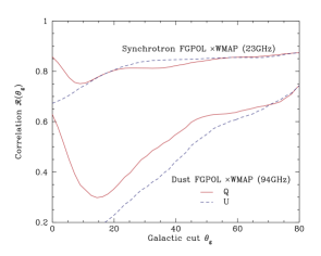
Figure 4: Comparison of the correlation coefficient $\cal R$ between the FGPol maps and WMAP best–fit templates for both synchrotron and dust. In order to look at the correlation on large scales we smooth these maps to a resolution of $10^{\circ}$. The correlation is calculated by including areas outside a range of cuts in Galactic latitude. The trend shows that both dust and synchrotron models are highly correlated with the best-fit maps at high Galactic latitudes whilst the correlation falls rapidly at low galactic latitudes for the dust comparison. The WMAP best–fit dust map however has an even larger noise residual than the synchrotron map and this is expected to reduce the correlation significantly.

We also attempt to quantify the level of correlation between the WMAP MCMC maps and FGPol templates. We do this using two separate measures. The first analyses the level of pixel-to-pixel correlation between maps calculated for the area of the sky outside a given galactic latitude cut. The correlation coefficient ${\cal R}$ is given by

$${\cal R}(\theta_{g}) =\frac{\sum_{p}({\cal W}_{p}-\widehat{\cal W}_{p})({\cal F}_{p}-\widehat{\cal F}_{p})}{\sqrt{\sum_{p}({\cal W}_{p}-\widehat{\cal W}_{p})^{2}\sum_{p}({\cal F}_{p}-\widehat{\cal F}_{p})^{2}}}\,.$$ (8)

where ${\cal W}$ and ${\cal F}$ are the $I$, $Q$, or $U$ Stokes values of the WMAP and FGPol maps respectively and the index $p$ sums over all pixels outside the cut at latitude $\pm\theta_{g}$. The result, for both dust and synchrotron $Q$ and $U$ Stokes parameters is shown in Figure 4. The analysis shows that both dust and synchrotron templates are highly correlated with the WMAP best-fit foreground templates at high Galactic latitudes. Whilst this is also true for synchrotron at low Galactic latitudes, the dust model fails to reproduce the observed morphology well at latitudes below $\sim$ 30 degrees. This is not surprising since thermal emission by dust particles is more susceptible to the detailed structure in the Galactic disk with even large angular scales being influenced by turbulence and/or existence of individual clouds.

We also look at the correlation in terms of scatter of the pixel values in $Q$ and $U$ Stokes parameters for the WMAP MCMC maps versus the FGPol templates in both dust and synchrotron. All pixels outside the P06 mask and MCMC flagged pixels are included and the scatter density is shown in Figure 5 as two contours encompassing 68% and 95% of pixels. We only show the synchrotron correlation density since the dust one is found to be dominated by the larger WMAP variance due to residual noise and is not informative.

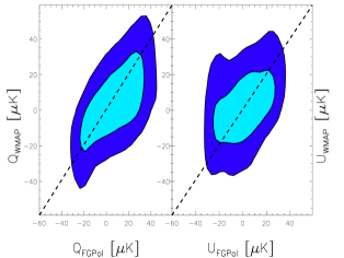
Figure 5: Comparison of the scatter between the FGPol maps and WMAP best–fit templates for synchrotron. This is done for the full–sky templates including pixels outside the combination of the P06 polarisation mask and WMAP MCMC flagged pixels. The dust correlation density is omitted as it is dominated by the variance in the WMAP map due to residual noise.

6 Foreground amplitudes in sub–orbital sky patches

We also examine the amplitude of foreground contamination in smaller sky areas being targeted by a sample of three currently operating or planned sub-orbital experiments; EBEX (Reichborn-Kjennerud et al., 2010), Spider (Filippini et al., 2010) and the Bicep2 and Keck (Orlando et al., 2010) arrays which observe the same field. Angular resolution and sensitivity for the three experiments are varied but they are all targeting the detection of $BB$ power either on large angular scales that are free of lensing effects or, as in the case of EBEX, on smaller angular scales where the lensing effect dominates the $BB$ signal.

We generate high resolution templates with full three-dimensional modelling of the turbulent small-scale GMF over the regions of expected coverage for the three experiments. For the dust templates, the $Q$ and $U$ components are normalised so that the average polarisation fraction outside the area defined by the WMAP P06 mask is 3.6%. The coverage areas are outlined in Figure 6 with Spider targeting the largest area with $f_{\rm sky}\sim 0.1$, EBEX targeting the smallest patch contained in the Spider area with $f_{\rm sky}\sim 0.01$ and Bicep2/Keck targeting the southern most patch with $f_{\rm sky}\sim 0.03$.

In order to compare the relative contamination by foregrounds in relation to the relevant signal we analyse the angular power spectrum $C_{\ell}^{BB}$ for both dust and synchrotron. Due to the uncertainties involved in predicting the small scale signal we focus on large scales only with templates smoothed to a common resolution of $1^{\circ}$ and rely on extrapolating a power law to scales larger than $\ell\sim 200$ in comparing with the expected signal.

The analysis on small areas of the sky such as these is complicated by the significant correlation induced by the cut on spherical harmonic coefficients. The high level of correlation would result in significant biases if the same power law fitting procedure as used in Section 5 were carried out. To avoid this problem we estimate the overall amplitude of foreground contamination by averaging in pixel space assuming a fixed power law in $\ell$ corresponding to our previous near full-sky analysis.

In practice we calculate the variance in both $Q$ and $U$ for each patch and assume a relation between the variance and angular power spectrum of the form

$$\sigma^{2}=\frac{1}{4\pi}\sum_{\ell=2}^{\ell_{\rm max}}(2\ell+1)C_{\ell}B^{2}_{\ell}(\theta_{s})\,,$$ (9)

with the signal angular power spectrum modelled as $C_{\ell}=A\,\ell^{m}$ in accordance with (7) and with index $m$ set to the corresponding near full-sky best-fit value (see Table 1). We take $\ell_{\rm max}=128$ and model the smoothing $B_{\ell}$ applied to the templates as a Gaussian beam with FWHM $1^{\circ}$ multiplied by the pixel window function at the working HealPix resolution $N_{\rm side}=64$. We then invert the relation (9) to obtain an ‘average’ polarisation angular power spectrum amplitude $A$, effectively assuming that power is equally distributed between $EE$ and $BB$.

The results are summarised in Figure 7 for a single reference frequency of 150 GHz as this is being included as an observing frequency in all experiments being considered. The model power spectra for each patch are shown in thermodynamic temperature in order to compare directly with the expected $BB$ signal for a tensor-to-scalar ratio $r=0.1$. Both primordial and lensing contribution to the $BB$ signal are shown.

The amplitude of foreground contamination varies by roughly an order of magnitude between the area targeted by different experiments. In particular the area targeted by EBEX seems to be very clean with the foreground signal reduced by an order of magnitude compared to the areas targeted by Spider and Bicep2/Keck. This agrees visually with the impression given in Figure 6.

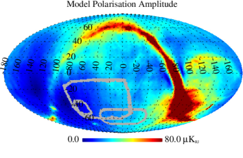
Figure 6: Comparison of patches targeted by a variety of sub-orbital experiments. Spider targets the largest area ($f_{\rm sky}\sim 0.1$), EBEX targets the smallest patch ($f_{\rm sky}\sim 0.01$) and Bicep2/Keck targets the southern most patch ($f_{\rm sky}\sim 0.03$).

7 Conclusions

We have presented templates for polarised emission from synchrotron radiation within our Galaxy using a 3D model of the Galactic magnetic field and cosmic ray density distribution. From this model, maps of polarisation amplitude and angle are calculated which are then combined with total intensity measurements from the Haslam 408MHz all-sky radio continuum survey to provide template maps.

We have compared the FGPol templates obtained from this model with data from the WMAP satellite for both synchrotron and dust emission. We find that the synchrotron template agrees qualitatively with the observations whereas comparison of the dust template is complicated by the large residuals present in the WMAP estimates.

We have also looked at foreground contamination levels in patches that will be targeted by upcoming experiments and found that our model predicts significant differences of up to an order of magnitude in the foreground contamination of different patches. The level of contamination will dominate the ability of various experiments to achieve their target sensitivity with respect to the $B$-mode signal being searched for.

As more polarisation data becomes available the comparison between the model and observations will become more quantitatively precise. In particular future Planck data releases will provide high signal-to-noise $Q$ and $U$ maps at a number of frequencies and we will be able to refine our model based on them. Indeed, in future, it should be possible to learn much about the Galactic magnetic field itself by fitting the (many) model parameters to actual data. This will shed light on many aspects of our Galaxy’s physical model that are still poorly understood.

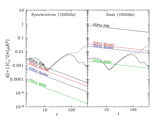
Figure 7: Foreground amplitude for synchrotron (left panel) and dust (right panel) calculated from patches targeted by various suborbital experiments compared with theoretical $EE$ and $BB$ spectra for $r=0.1$. The index of the power law used is from the corresponding near full sky power spectrum fits. Also shown are the near full sky best fit spectra for the FGPol synchrotron template from Table 1 along with best fit spectra to the dust templates with $Q$ and $U$ normalised so that the polarisation fraction is 3.6% outside the WMAP P06 mask. The amplitudes were calculated from our FGPol dust and synchrotron templates at 150GHz calculated from maps generated at $N_{\rm side}=1024$ for the large scale resolution and $N_{\rm side}^{\rm P}=128$ for the small scale line-of-sight resolution, which are then smoothed to $1^{\circ}$ and downgraded to $N_{\rm side}=64$. Units are $\mu K_{\rm CMB}$.

References

- Armitage-Caplan et al. (2012) Armitage-Caplan C., Dunkley J., Eriksen H. K., Dickinson C., 2012
- Bennett et al. (2003) Bennett C. L. et al., 2003, ApJS, 148, 97
- Benoît et al. (2004) Benoît A. et al., 2004, A&A, 424, 571
- Delabrouille et al. (2012) Delabrouille J., Betoule M., Melin J.-B., Miville-Deschenes M.-A., Gonzalez-Nuevo J., et al., 2012
- Dickinson, Davies & Davis (2003) Dickinson C., Davies R., Davis R., 2003, Mon.Not.Roy.Astron.Soc., 341, 369
- Dodelson et al. (2009) Dodelson S., Easther R., Hanany S., McAllister L., Meyer S., et al., 2009
- Drimmel & Spergel (2001) Drimmel R., Spergel D. N., 2001, ApJ, 556, 181
- Essinger-Hileman et al. (2010) Essinger-Hileman T. et al., 2010, ArXiv e-prints
- Fauvet et al. (2010) Fauvet L., Macias-Perez J., Aumont J., Desert F., Jaffe T., et al., 2010
- Filippini et al. (2010) Filippini J. P. et al., 2010, Proc. SPIE, 7741, 77411N
- Gold et al. (2011) Gold B., Odegard N., Weiland J., Hill R., Kogut A., et al., 2011, Astrophys.J.Suppl., 192, 15
- Gold et al. (2011) Gold B. et al., 2011, ApJS, 192, 15
- Górski et al. (2005) Górski K. M., Hivon E., Banday A. J., Wandelt B. D., Hansen F. K., Reinecke M., Bartelmann M., 2005, ApJ, 622, 759
- Haslam et al. (1982) Haslam C., Salter C., Stoffel H., Wilson W., 1982, Astron.Astrophys.Suppl.Ser., 47, 1
- Hinshaw et al. (2007) Hinshaw G. et al., 2007, ApJS, 170, 288
- Jarosik et al. (2011) Jarosik N., Bennett C., Dunkley J., Gold B., Greason M., et al., 2011, Astrophys.J.Suppl., 192, 14
- Longair (1994) Longair M. S., 1994, High energy astrophysics. Volume 2. Stars, the Galaxy and the interstellar medium.
- López-Caraballo et al. (2011) López-Caraballo C. H., Rubiño-Martín J. A., Rebolo R., Génova-Santos R., 2011, ApJ, 729, 25
- Macellari et al. (2011) Macellari N., Pierpaoli E., Dickinson C., Vaillancourt J., 2011, ArXiv e-prints
- Miville-Deschenes et al. (2008) Miville-Deschenes M. ., Ysard N., Lavabre A., Ponthieu N., Macias-Perez J. F., Aumont J., Bernard J. P., 2008, ArXiv preprint
- O’Dea (2009) O’Dea D. T., 2009, PhD thesis, University of Cambridge, UK
- O’Dea et al. (2011) O’Dea D. T. et al., 2011, ApJ, 738, 63
- O’Dea et al. (2012) O’Dea D. T., Clark C. N., Contaldi C. R., MacTavish C. J., 2012, MNRAS, 419, 1795
- Orlando et al. (2010) Orlando A., Aikin R., Amiri M., Bock J., Bonetti J., et al., 2010
- Page et al. (2007) Page L. et al., 2007, ApJS, 170, 335
- Peel et al. (2011) Peel M., Dickinson C., Davies R., Banday A., Jaffe T., et al., 2011
- Reichborn-Kjennerud et al. (2010) Reichborn-Kjennerud B. et al., 2010, in Society of Photo-Optical Instrumentation Engineers (SPIE) Conference Series, Vol. 7741, Society of Photo-Optical Instrumentation Engineers (SPIE) Conference Series
- Rybicki & Lightman (1979) Rybicki G. B., Lightman A. P., 1979, Radiative processes in astrophysics
- Sheehy et al. (2011) Sheehy C. D. et al., 2011, ArXiv e-prints
- Spoelstra (1984) Spoelstra T. A. T., 1984, A&A, 135, 238
- The Polarbear Collaboration et al. (2010) The Polarbear Collaboration et al., 2010, ArXiv e-prints