The Metallicity Evolution of Star-Forming Galaxies from redshift 0 to 3: Combining Magnitude Limited Survey with Gravitational Lensing

Abstract

We present a comprehensive observational study of the gas phase metallicity of star-forming galaxies from $z\sim 0\rightarrow 3$. We combine our new sample of gravitationally lensed galaxies with existing lensed and non-lensed samples to conduct a large investigation into the mass-metallicity (MZ) relation at $z>1$. We apply a self-consistent metallicity calibration scheme to investigate the metallicity evolution of star-forming galaxies as a function of redshift. The lensing magnification ensures that our sample spans an unprecedented range of stellar mass (3 $\times$ 10⁷$-$6$\times$10¹⁰ M_⊙). We find that at the median redshift of $z=2.07$, the median metallicity of the lensed sample is 0.35 dex lower than the local SDSS star-forming galaxies and 0.18 dex lower than the $z\sim 0.8$ DEEP2 galaxies. We also present the $z\sim 2$ MZ relation using 19 lensed galaxies. A more rapid evolution is seen between $z\sim 1\rightarrow 3$ than $z\sim 0\rightarrow 1$ for the high-mass galaxies (10^9.5 M${}_{\odot}<$M${}_{\star}<$10¹¹ M_⊙), with almost twice as much enrichment between $z\sim 1\rightarrow 3$ than between $z\sim 1\rightarrow 0$. We compare this evolution with the most recent cosmological hydrodynamic simulations with momentum driven winds. We find that the model metallicity is consistent with the observed metallicity within the observational error for the low mass bins. However, for higher masses, the model over-predicts the metallicity at all redshifts. The over-prediction is most significant in the highest mass bin of 10^10-11 M_⊙.

1. Introduction

Soon after the pristine clouds of primordial gas collapsed to assemble a protogalaxy, star formation ensued, leading to the production of heavy elements (metals). Metals were synthesized exclusively in stars, and were ejected into the interstellar medium (ISM) through stellar winds or supernovae explosions. Tracing the heavy element abundance (metallicity) in star-forming galaxies provides a “fossil record” of galaxy formation and evolution.

When considered as a closed system, the metal content of a galaxy is directly related to the yield and gas fraction (Searle & Sargent, 1972; Pagel & Patchett, 1975; Pagel & Edmunds, 1981; Edmunds, 1990). In reality, a galaxy interacts with its surrounding intergalactic medium (IGM), hence both the overall and local metallicity distribution of a galaxy is modified by feedback processes such as galactic winds, inflows, and gas accretions (e.g., Lacey & Fall, 1985; Edmunds & Greenhow, 1995; Köppen & Edmunds, 1999; Dalcanton, 2007). Therefore, observations of the chemical abundances in galaxies offer crucial constraints on the star formation history and various mechanisms responsible for galactic inflows and outflows.

The well-known correlation between galaxy mass (luminosity) and metallicity was first proposed by Lequeux et al. (1979). Subsequent studies confirmed the existence of the luminosity-metallicity (LZ) relation (e.g., Rubin et al., 1984; Skillman et al., 1989; Zaritsky et al., 1994; Garnett, 2002). Luminosity was used as a proxy for stellar mass in these studies as luminosity is a direct observable. Aided by new sophisticated stellar population models, stellar mass can be robustly calculated and a tighter correlation is found in the mass-metallicity (MZ) relation. Tremonti et al. (2004) have established the MZ relation for local star-forming galaxies based on $\sim$ 5$\times$10⁵ Sloan Digital Sky Survey (SDSS) galaxies. At intermediate redshifts ($0.4<z<1$), the MZ relation has also been observed for a large number of galaxies ($>$100) (e.g., Savaglio et al., 2005; Cowie & Barger, 2008; Lamareille et al., 2009). Zahid et al. (2011) derived the MZ relation for $\sim$ 10³ galaxies from the Deep Extragalactic Evolutionary Probe 2 (DEEP2) survey, validating the MZ relation on a statistically significant level at $z\sim 0.8$.

Current cosmological hydrodynamic simulations and semi-analytical models can predict the metallicity history of galaxies on a cosmic timescale (Nagamine et al., 2001; De Lucia et al., 2004; Bertone et al., 2007; Brooks et al., 2007; Davé & Oppenheimer, 2007; Davé et al., 2011a, b). These models show that the shape of the MZ relation is particularly sensitive to the adopted feedback mechanisms. The cosmological hydrodynamic simulations with momentum-driven winds models provide better match with observations than energy-driven wind models (Oppenheimer & Davé, 2008; Finlator & Davé, 2008; Davé et al., 2011a). However, these models have not been tested thoroughly in observations, especially at high redshifts ($z>1$), where the MZ relation is still largely uncertain.

As we move to higher redshifts, selection effects and small number statistics haunt observational metallicity history studies. The difficulty becomes more severe in the so-called “redshift desert” ($1\lesssim z\lesssim 3$), where the metallicity sensitive optical emission lines have shifted to the sky-background dominated near infrared (NIR). Ironically, this redshift range harbors the richest information about galaxy evolution. It is during this redshift period ($\sim$ 2$-$6 Gyrs after the Big Bang) that the first massive structures condensed; the star formation rate (SFR), major merger activity, and black hole accretion rate peaked; much of today’s stellar mass was assembled, and heavy elements were produced (Fan et al., 2001; Dickinson et al., 2003; Chapman et al., 2005; Hopkins & Beacom, 2006; Grazian et al., 2007; Conselice et al., 2007; Reddy et al., 2008). It is therefore of crucial importance to explore NIR spectra for galaxies in this redshift range.

Many spectroscopic redshift surveys have been carried out to study star-forming galaxies at $z>$1 in recent years (e.g., Steidel et al., 2004; Law et al., 2009). However, due to the low efficiency in the NIR, those spectroscopic surveys almost inevitably have to rely on color-selection criteria and the biases in UV-selected galaxies tend to select the most massive and less dusty systems (e.g., Capak et al., 2004; Steidel et al., 2004; Reddy et al., 2006). Space telescopes can observe much deeper in the NIR and are able to probe a wider mass range. For example, the narrow-band H$\alpha$ surveys based on the new WFC3 camera aboard the Hubble Space Telescope (HST) have located hundreds of H$\alpha$ emitters up to z = 2.23, finding much fainter systems than observed from the ground (Sobral et al., 2009). However, the low-resolution spectra from the narrow band filters forbid derivations of physical properties such as metallicities that can only currently be acquired from ground-based spectral analysis.

Thanks to the advent of long-slit/multi-slit NIR spectrographs on 8$-$10 meter class telescopes, enormous progress has been made in the last decade to capture galaxies in the redshift desert. For chemical abundance studies, a full coverage of rest-frame optical spectra (4000$-$9000$\AA$) is usually mandatory for the most robust diagnostic analysis. For 1.5 $\lesssim z\lesssim 3$, the rest-frame optical spectra have shifted into the J, H, and K bands. It remains challenging and observationally expensive to obtain high signal-to-noise ($S/N$) NIR spectra from the ground, especially for “typical” targets at high-$z$ that are less massive than conventional color-selected galaxies. Therefore, previous investigations into the metallicity properties between $1\lesssim z\lesssim 3$ focused on stacked spectra, samples of massive luminous individual galaxies, or very small numbers of lower-mass galaxies (e.g., Erb et al., 2006; Förster Schreiber et al., 2006; Law et al., 2009; Erb et al., 2010; Yabe et al., 2012).

The first mass-metallicity (MZ) relation for galaxies at z $\sim$ 2 was found by Erb et al. (2006) using the stacked spectra of 87 UV selected galaxies divided into 6 mass bins. Subsequently, mass and metallicity measurements have been reported for numerous individual galaxies at 1.5 $<z<$ 3 (Förster Schreiber et al., 2006; Genzel et al., 2008; Hayashi et al., 2009; Law et al., 2009; Erb et al., 2010). These galaxies are selected using broadband colors in the UV (Lyman Break technique; Steidel et al., 1996, 2003) or using B, z, and K-band colors (BzK selection; Daddi et al., 2004). The Lyman break and BzK selection techniques favor galaxies that are luminous in the UV or blue and may therefore be biased against low luminosity (low-metallicity) galaxies, and dusty (potentially metal-rich) galaxies. Because of these biases, galaxies selected in this way may not sample the full range in metallicity at redshift z $>$1.

A powerful alternative method to avoid these selection effects is to use strong gravitationally lensed galaxies. In the case of galaxy cluster lensing, the total luminosity and area of the background sources can easily be boosted by $\sim 10-50$ times, providing invaluable opportunities to obtain high S/N spectra and probe intrinsically fainter systems within a reasonable amount of telescope time. In some cases, sufficient S/N can even be obtained for spatially resolved pixels to study the resolved metallicity of high-$z$ galaxies (Swinbank et al., 2009; Jones et al., 2010; Yuan et al., 2011; Jones et al., 2012). Before 2011, metallicities have been reported for a handful of individually lensed galaxies using optical emission lines at 1.5 $<z<$ 3 (Pettini et al., 2001; Lemoine-Busserolle et al., 2003; Stark et al., 2008; Quider et al., 2009; Yuan & Kewley, 2009; Jones et al., 2010). Fortunately, lensed galaxy samples with metallicity measurements have increased significantly thanks to reliable lensing mass modeling and larger dedicated spectroscopic surveys of lensed galaxies on 8-10 meter telescopes (Richard et al., 2011; Wuyts et al., 2012; Christensen et al., 2012).

In 2008, we began a spectroscopic observational survey designed specifically to capture metallicity sensitive lines for lensed galaxies. Taking advantage of the multi-object cryogenic NIR spectrograph (MOIRCS) on Subaru, we targeted well-known strong lensing galaxy clusters to obtain metallicities for galaxies between 0.8 $<z<$ 3. In this paper, we present the first metallicity measurement results from our survey.

Combining our new data with existing data from the literature, we present a coherent observational picture of the metallicity history and mass-metallicity evolution of star-forming galaxies from $z\sim 0$ to $z\sim 3$. Kewley & Ellison (2008) have shown that the metallicity offsets in the diagnostic methods can easily exceed the intrinsic trends. It is of paramount importance to make sure that relative metallicities are compared on the same metallicity calibration scale. In MZ relation studies, the methods used to derive the stellar mass can also cause systematic offsets (Zahid et al., 2011). Different SED fitting codes can yield a non-negligible mass offset, hence mimicking or hiding evolution in the MZ relation. In this paper, we derive the mass and metallicity of all samples using the same methods, ensuring that the observational data are compared in a self-consistent way. We compare our observed metallicity history with the latest prediction from cosmological hydrodynamical simulations.

Throughout this paper we use a standard $\Lambda$CDM cosmology with $H_{0}$= 70 km s^-1 Mpc^-1, $\Omega_{M}$=0.30, and $\Omega_{\Lambda}$=0.70. We use solar oxygen abundance 12 + log(O/H)_⊙=8.69 (Asplund et al., 2009).

The paper is organized as follows: Section 2 describes our lensed sample survey and observations. Data reduction and analysis are summarized in Section 3. Section 4 presents an overview of all the samples we use in this study. Section 5 describes the methodology of derived quantities. The metallicity evolution of star-forming galaxies with redshift is presented in Section 6. Section 7 presents the mass-metallicity relation for our lensed galaxies. Section 8 compares our results with previous work in literature. Section 9 summarizes our results. In the Appendix, we show the morphology, slit layout, and reduced 1D spectra for the lensed galaxies reported in our survey.

2. The LEGMS survey and Observations

Table 1MOIRCS Observation Summary

Target	Dates	Exposure Time	PA	Seeing($K_{s}$)	Slit width	Filter/Grism
		(ks)	(deg)	$\!\!{}^{\prime\prime}$	$\!\!{}^{\prime\prime}$
Abell 1689	Apr 28,2011	50.0	60	0.5-0.8	$\cdots$	Ks Imaging
Abell 1689	Apr 28,2010	15.6	-60	0.5-0.8	0.8	HK500
Abell 1689	Apr 29,2010	19.2	45	0.5-0.6	0.8	HK500
Abell 1689	Mar 24,2010	16.8	20	0.5-0.6	0.8	HK500
Abell 1689	Mar 25,2010	12.0	-20	0.6-0.7	0.8	HK500
Abell 1689	Apr 23, Mar 24, 2008	15.6	60	0.5-0.8	0.8	zJ500
Abell 68	Sep 29-30,2009	12.0	60	0.6-1.0	1.0	HK500, zJ500

Note. — Log of the observations. We use a dithering length of 2.$\!\!{}^{\prime\prime}$5 for all the spectroscopic observations.

2.1. The Lensed Emission-Line Galaxy Metallicity Survey (LEGMS)

Our survey (LEGMS) aims to obtain oxygen abundance of lensed galaxies at 0.8$<$z$<$3. LEGMS has taken enormous advantage of the state-of-the-art instruments on Mauna Kea. Four instruments have been utilized so far: (1) the Multi-Object InfraRed Camera and Spectrograph (MOIRCS; Ichikawa et al. 2006) on Subaru; (2) the OH-Suppressing Infra-Red Imaging Spectrograph (OSIRIS; Larkin et al. 2006) on Keck II; (3) the Near Infrared Spectrograph (NIRSPEC; McLean et al. 1998) on Keck II; (4) the Low Dispersion Imaging Spectrograph (LRIS; Oke et al. 1995) on Keck I. The scientific objective of each instrument is as follows: MOIRCS is used to obtain the NIR images and spectra for multiple targets behind lensing clusters; NIRSPEC is used to capture occasional single field lensed targets (especially galaxy-scale lenses); LRIS is used to obtain the [O ii]$\,\lambda$3727 to [O iii]$\,\lambda$5007 spectral range for targets with z $<$ 1.5. From the slit spectra, we select targets that are have sufficient fluxes and angular sizes to be spatially resolved with OSIRIS. In this paper we focus on the MOIRCS observations of the lensing cluster Abell 1689 for targets between redshifts 1.5 $\lesssim$ z $\lesssim$ 3. Observations for other clusters are ongoing and will be presented in future papers.

The first step to construct a lensed sample for slit spectroscopy is to find the lensed candidates (arcs) that have spectroscopic redshifts from optical surveys. The number of known spectroscopically identified lensed galaxies at z $>$ 1 is still on the order of a few tens. The limited number of lensed candidates makes it impractical to build a sample that is complete and well defined in mass. A mass complete sample is the future goal of this project. Our strategy for now is to observe as many arcs with known redshifts as possible. If we assume the AGN fraction is similar to local star-forming galaxies, then we expect $\sim$ 10% of our targets to be AGN dominated (Kewley et al., 2004). Naturally, lensed sample is biased towards highly magnified sources. However, because the largest magnifications are not biased towards intrinsically bright targets, lensed samples are less biased towards the intrinsically most luminous galaxies.

Abell 1689 is chosen as the primary target for MOIRCS observations because it has the largest number ($\sim$ 100 arcs, or $\sim$ 30 source galaxies) of spectroscopically identified lensed arcs (Broadhurst et al., 2005; Frye et al., 2007; Limousin et al., 2007).

Multi-slit spectroscopy of NIR lensing surveys greatly enhances the efficiency of spectroscopy of lensed galaxies in clusters. Theoretically, $\sim$ 40 slits can be observed simultaneously on the two chips of MOIRCS with a total field of view (FOV) of 4${}^{\prime}\times 7^{\prime}$. In practice, the number of lensed targets on the slits is restricted by the strong lensing area, slit orientations, and spectral coverage. For A1689, the lensed candidates cover an area of $\sim$2^′ $\times$ 2^′, well within the FOV of one chip. We design slit masks for chip 2, which has better sensitivity and less bad pixels than chip 1. There are $\sim$ 40 lensed images ($\sim$ 25 individual galaxies) that fall in the range of 1.5 $\lesssim$ z $\lesssim$ 3 in our slit masks. We use the MOIRCS low-resolution (R$\sim$ 500) grisms which have a spectral coverage of 0.9 -1.78 $\mu$m in ZJ and 1.3-2.5 $\mu$m in HK. To maximize the detection efficiency, we give priority to targets with the specific redshift range such that all the strong emission lines from [O ii]$\,\lambda$3727 to [N ii]$\,\lambda$6584 can be captured in one grism configuration. For instance, the redshift range of 2.5 $\lesssim$ z $\lesssim$ 3 is optimized for the HK500 grism, and 1.5 $\lesssim$ z $\lesssim$ 1.7 is optimized for the ZJ500 grism.

From UT March 2008 to UT April 2010, we used 8 MOIRCS nights (6 usable nights) with 4 position angles (PAs) and 6 masks to observe 25 galaxies. Metallicity quality spectra were obtained for 12 of the 25 targets. We also include one $z>1.5$ galaxy from our observations of Abell 68. The PA is chosen to optimize the slit orientation along the targeted arcs’ elongated directions. For arcs that are not oriented to match the PA, the slits are configured to center on the brightest knots of the arcs. We use slit widths of 0.8 $\!\!{}^{\prime\prime}$ and 1.0 $\!\!{}^{\prime\prime}$, with a variety of slit lengths for each lensed arc. For each mask, a bright galaxy/star is placed on one of the slits to trace the slit curvature and determine the offsets among individual exposures. Typical integrations for individual frames are 400 s, 600 s, and 900 s, depending on levels of skyline saturation. We use an ABBA dithering sequence along the slit direction, with a dithering length of 2.$\!\!{}^{\prime\prime}$5. The observational logs are summarized in Table 1.

3. Data Reduction and Analysis

3.1. Reduce 1D spectrum

The data reduction procedures from the raw mask data to the final wavelength and flux calibrated 1D spectra were realized by a set of IDL codes called MOIRCSMOSRED. The codes were scripted originally by Youichi Ohyama. T.-T Yuan extended the code to incorporate new skyline subtraction (e.g., Henry et al., 2010, for a description of utilizing MOIRCSMOSRED).

We use the newest version (Apr, 2011) of MOIRCSMOSRED to reduce the data in this work. The sky subtraction is optimized as follows. For each A_i frame, we subtract a sky frame denoted as $\alpha$((B_i-1+B_i+1)/2), where B_i-1 and B_i+1 are the science frames before and after the A_i exposure. The scale parameter $\alpha$ is obtained by searching through a parameter range of 0.5-2.0, with an increment of 0.0001. The best $\alpha$ is obtained where the root mean square (RMS) of the residual R$=$ A_i- $\alpha$((B_i-1+B_i+1)/2) is minimal for a user defined wavelength region $\lambda_{1}$ and $\lambda_{2}$. We find that this sky subtraction method yields smaller sky OH line residuals ($\sim$ 20%) than conventional A-B methods. We also compare with other skyline subtraction methods in literature (Kelson, 2003; Davies, 2007). We find the sky residuals from our method are comparable to those from the Kelson (2003) and Davies (2007) methods within 5% in general cases. However, in cases where the emission line falls on top of a strong skyline, our method is more stable and improves the skyline residual by $\sim$ 10% than the other two methods.

Wavelength calibration is carried out by identifying skylines for the ZJ grism. For the HK grism, we use argon lines to calibrate the wavelength since only a few skylines are available in the HK band. The argon-line calibrated wavelength is then re-calibrated with the available skylines in HK to determine the instrumentation shifts between lamp and science exposures. Note that the RMS of the wavelength calibration using a 3rd order polynomial fitting is $\sim$ 10-20 Å, corresponding to a systematic redshift uncertainty of 0.006.

A sample of A0 stars selected from the UKIRT photometric standards were observed at similar airmass as the targets. These stars were used for both telluric absorption corrections and flux calibrations. We use the prescriptions of Erb et al. (2003) for flux calibration. As noted in Erb et al. (2003), the absolute flux calibration in the NIR is difficult with typical uncertainties of $\sim$20%. We note that this uncertainty is even larger for lensed samples observed in multi-slits because of the complicated aperture effects. The uncertainties in the flux calibration are not a concern for our metallicity analysis where only line ratios are involved. However, these errors are a major concern for calculating SFRs. The uncertainties from the multi-slit aperture effects can cause the SFRs to change by a factor of 2-3. For this reason, we refrain from any quantitative analysis of SFRs in this work.

3.2. Line Fitting

The emission lines are fitted with Gaussian profiles. For the spatially unresolved spectra, the aperture used to extract the spectrum is determined by measuring the Gaussian profile of the wavelength collapsed spectrum. Some of the lensed targets ($\sim$ 10%) are elongated and spatially resolved in the slit spectra, however, because of the low surface brightness and thus very low S/N per pixel, we are unable to obtain usable spatially resolved spectra. For those targets, we make an initial guess for the width of the spatial profile and force a Gaussian fit, then we extract the integrated spectrum using the aperture determined from the FWHM of the Gaussian profile.

For widely separated lines such as [O ii]$\,\lambda$3727, H$\beta$$\,\lambda$4861, single Gaussian functions are fitted with 4 free parameters: the centroid (or the redshift), the line width, the line flux, and the continuum. The doublet [O iii]$\,\lambda$$\,\lambda$4959,5007 are initially fitted as a double Gaussian function with 6 free parameters: the centroids 1 and 2 , line widths 1 and 2, fluxes 1 and 2, and the continuum. In cases where the [O iii]$\,\lambda$4959 line is too weak, its centroid and line velocity width are fixed to be the same as [O iii]$\,\lambda$5007 and the flux is fixed to be 1/3 of the [O iii]$\,\lambda$5007 line (Osterbrock, 1989). A triple-Gaussian function is fitted simultaneously to the three adjacent emission lines: [N ii]$\,\lambda$6548, 6583 and H$\alpha$. The centroid and velocity width of [N ii]$\,\lambda$6548, 6583 lines are constrained by the velocity width of H$\alpha$$\,\lambda$6563, and the ratio of [N ii]$\,\lambda$6548 and [N ii]$\,\lambda$6583 is constrained to be the theoretical value of 1/3 given in Osterbrock (1989). The line profile fitting is conducted using a $\chi^{2}$ minimization procedure which uses the inverse of the sky OH emission as the weighting function. The S/N per pixel is calculated from the $\chi^{2}$ of the fitting. The measured emission line fluxes and line ratios are listed in Table 4. The final reduced 1D spectra are shown in the Appendix.

3.3. Lensing Magnification

Because the lensing magnification ($\mu$) is not a direct function of wavelength, line ratio measurements do not require pre-knowledge of the lensing magnification. However, $\mu$ is needed for inferring other physical properties such as the intrinsic fluxes, masses and source morphologies. Parametric models of the mass distribution in the clusters Abell 68 and Abell 1689 were constructed using the Lenstool software Lenstool (Kneib et al., 1993; Jullo et al., 2007). The best-fit models have been previously published in Richard et al. (2007) and Limousin et al. (2007). As detailed in Limousin et al. (2007), Lenstool uses Bayesian optimization with a Monte-Carlo Markov Chain (MCMC) sampler which provides a family of best models sampling the posterior probability distribution of each parameter. In particular, we use this family of best models to derive the magnification and relative error on magnification $\mu$ associated to each lensed source. Typical errors on $\mu$ are $\sim$10% for Abell 1689 and Abell 68.

3.4. Photometry

We determine the photometry for the lensed galaxies in A1689 using 4-band HST imaging data, 1-band MOIRCS imaging data, and 2-channel Spitzer IRAC data at 3.6 and 4.5 $\mu$m.

We obtained a 5,000 s image exposure for A1689 on the MOIRCS K_s filter, at a depth of 24 mag, using a scale of 0.117 $\!\!{}^{\prime\prime}$ per pixel. The image was reduced using MCSRED in IRAF written by the MOIRCS supporting astronomer Ichi Tanaka. The photometry is calibrated using the 2MASS stars located in the field.

The ACS F475W, F625W, F775W, F850LP data are obtained from the HST archive. The HST photometry are determined using SExtractor (Bertin & Arnouts, 1996) with parameters adjusted to detect the faint background sources. The F775W filter is used as the detection image using a 1.$\!\!{}^{\prime\prime}$0 aperture.

The IRAC data are obtained from the Spitzer archive and are reduced and drizzled to a pixel scale of 0.$\!\!{}^{\prime\prime}$6 pixel^-1. In order to include the IRAC photometry, we convolved the HST and MOIRCS images with the IRAC point spread functions (PSFs) derived from unsaturated stars. All photometric data are measured using a 3.$\!\!{}^{\prime\prime}$0 radius aperture. Note that we only consider sources that are not contaminated by nearby bright galaxies: $\sim 70\%$ of our sources have IRAC photometry (Table 5). Typical errors for the IRAC band photometry are 0.3 mag, with uncertainties mainly from the aperture correction and contamination of neighboring galaxies. Typical errors for the ACS and MOIRCS bands are 0.15 mag, with uncertainties mainly from the Poisson noise and absolute zero-point uncertainties (Wuyts et al., 2012). We refer to Richard et al. (2012, in prep) for the full catalog of the lensing magnification and photometry of the lensed sources in Abell 1689.

4. Supplementary Samples

In addition to our lensed targets observed in LEGMS, we also include literature data for complementary lensed and non-lensed samples at both local and high-$z$. The observational data for individually measured metallicities at z $>$ 1.5 are still scarce and caution needs to be taken when using them for comparison. The different metallicity and mass derivation methods used in different samples can give large systematic discrepancies and provide misleading results. For this reason, we only include the literature data that have robust measurements and sufficient data for consistently recalculating the stellar mass and metallicities using our own methods. Thus, in general, stacked data, objects with lower/upper limits in either line ratios or masses are not chosen. The one exception is the stacked data of Erb et al. (2006), as it is the most widely used comparison sample at $z\sim 2$.

The samples used in this work are:

(1) The Sloan Digital Sky Survey (SDSS) sample ($z\sim$ 0.07). We use the SDSS sample (Abazajian et al., 2009, http://www.mpa-garching.mpg.de/SDSS/DR7/) defined by Zahid et al. (2011). The mass derivation method used in Zahid et al. (2011) is the same as we use in this work. All SDSS metallicities are recalculated using the PP04N2 method, which uses an empirical fit to the [N ii] and H$\alpha$ line ratios of H ii regions (Pettini & Pagel, 2004).

(2) The The Deep Extragalactic Evolutionary Probe 2 (DEEP2) sample ($z\sim$ 0.8). The DEEP2 sample (Davis et al., 2003, http://www.deep.berkeley.edu/DR3/) is defined in Zahid et al. (2011). At $z\sim$ 0.8, the [N ii] and H$\alpha$  lines are not available in the optical. We convert the KK04 R₂₃ metallicity to the PP04N2 metallicity using the prescriptions of Kewley & Ellison (2008).

(3) The UV-selected sample ($z\sim$ 2). We use the stacked data of Erb et al. (2006). The metallicity diagnostic used by Erb et al. (2006) is the PP04N2 method and no recalculation is needed. We offset the stellar mass scale of Erb et al. (2006) by -0.3 dex to match the mass derivation method used in this work (Zahid et al., 2012). This offset accounts for the different initial mass function (IMF) and stellar evolution model parameters applied by Erb et al. (2006).

(4) The lensed sample (1 $<$ z $<$ 3). Besides the 11 lensed galaxies from our LEGMS survey in Abell 1689, we include 1 lensed source ($z=$1.762) from our MOIRCS data on Abell 68 and 1 lensed spiral ($z=$1.49) from Yuan et al. (2011). We also include 10 lensed galaxies from Wuyts et al. (2012) and 3 lensed galaxies from Richard et al. (2011), since these 13 galaxies have [N ii] and H$\alpha$ measurements, as well as photometric data for recalculating stellar masses. We require all emission lines from literature to have S/N $>$ 3 for quantifying the metallicity of 1 $<$ z $<$ 3 galaxies. Upper-limit metallicities are found for 6 of the lensed targets from our LEGMS survey. Altogether, the lensed sample is composed of 25 sources, 12 (6/12 upper limits) of which are new observations from this work. Upper-limit metallicities are not used in our quantitative analysis.

The methods used to derive stellar mass and metallicity are discussed in detail in Section 5.

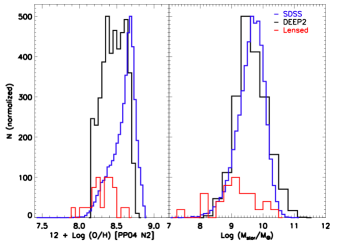
Figure 1.— Left panel: the metallicity distribution of the local SDSS (blue), intermediate-$z$ DEEP2 (black), and high-$z$ lensed galaxy samples (red). Right panel: the stellar mass distribution of the same samples. To present all three samples on the same figure, the SDSS (20577 points) and DEEP2 (1635 points) samples are normalized to 500, and the lensed sample (25 points) is normalized to 100.

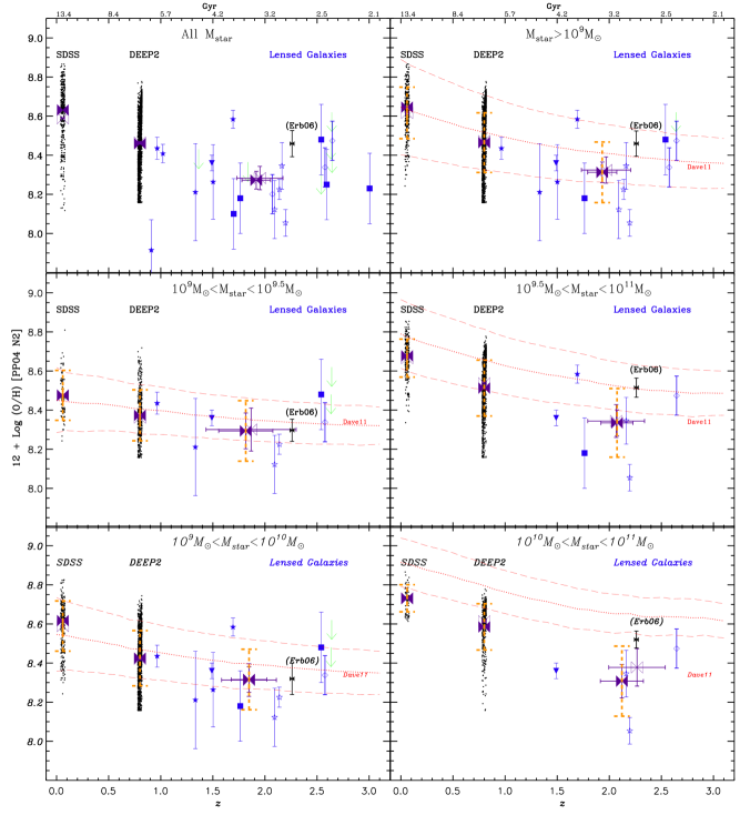
Figure 2.— The $\rm{Z}\emph{z}$ plot: metallicity history of star-forming galaxies from redshift 0 to 3. The SDSS and DEEP2 samples (black dots) are taken from Zahid et al. (2011). The SDSS data are plotted in bins to reduce visual crowdedness. The lensed galaxies are plotted in blue (upper-limit objects in green arrows), with different lensed samples showing in different symbols (see Figure 6 for the legends of the different lensed samples). The purple “bowties” show the bootstrapping mean (filled symbol) and median (empty symbol) metallicities and the 1$\sigma$ standard deviation of the mean and median, whereas the orange dashed error bars show the 1$\sigma$ scatter of the data. For the SDSS and DEEP2 samples, the $1\sigma$ errors of the median metallicities are 0.001 and 0.006 (indiscernible from the figure), whereas for the lensed sample the $1\sigma$ scatter of the median metallicity is 0.067. Upper limits are excluded from the median and error calculations. For comparison, we also show the mean metallicity of the UV-selected galaxies from Erb et al. (2006) (symbol: the black bowtie). The 6 panels show samples in different mass ranges. The red dotted and dashed lines are the model predicted median and $1\sigma$ scatter (defined as including 68% of the data) of the SFR-weighted gas metallicity in simulated galaxies (Davé et al., 2011b).

5. Derived Quantities

5.1. Optical Classification

We use the standard optical diagnostic diagram (BPT) to exclude targets that are dominated by AGN (Baldwin et al., 1981; Veilleux & Osterbrock, 1987; Kewley et al., 2006). For all 26 lensed targets in our LEGMS sample, we find 1 target that could be contaminated by AGN (B8.2). The fraction of AGN in our sample is therefore $\sim$8%, which is similar to the fraction ($\sim$7%) of the local SDSS sample (Kewley et al., 2006). We also find that the line ratios of the high-z lensed sample has a systematic offset on the BPT diagram, as found in Shapley et al. (2005); Erb et al. (2006); Kriek et al. (2007); Brinchmann et al. (2008); Liu et al. (2008); Richard et al. (2011). The redshift evolution of the BPT diagram will be reported in Kewley et al (2013, in preparation).

5.2. Stellar Masses

We use the software LE PHARE (Ilbert et al., 2009) to determine the stellar mass. LE PHARE is a photometric redshift and simulation package based on the population synthesis models of Bruzual & Charlot (2003). If the redshift is known and held fixed, LE PHARE finds the best fitted SED on a $\chi^{2}$ minimization process and returns physical parameters such as stellar mass, SFR and extinction. We choose the initial mass function (IMF) by Chabrier (2003) and the Calzetti et al. (2000) attenuation law, with E$\rm{(B-V)}$ ranging from 0 to 2 and an exponentially decreasing SFR (SFR $\varpropto$ e^-t/τ) with $\tau$ varying between 0 and 13 Gyrs. The errors caused by emission line contamination are taken into account by manually increasing the uncertainties in the photometric bands where emission lines are located. The uncertainties are scaled according to the emission line fluxes measured by MOIRCS. The stellar masses derived from the emission line corrected photometry are consistent with those without emission line correction, albeit with larger errors in a few cases ($\sim$ 0.1 dex in log space). We use the emission-line corrected photometric stellar masses in the following analysis.

5.3. Metallicity Diagnostics

The abundance of oxygen (12 + log(O/H)) is used as a proxy for the overall metallicity of H ii regions in galaxies. The oxygen abundance can be inferred from the strong recombination lines of hydrogen atoms and collisionally excited metal lines (e.g., Kewley & Dopita, 2002). Before doing any metallicity comparisons across different samples and redshifts, it is essential to convert all metallicities to the same base calibration. The discrepancy among different diagnostics can be as large as 0.7 dex for a given mass, large enough to mimic or hide any intrinsic observational trends. Kewley & Ellison (2008) (KE08) have shown that both the shape and the amplitude of the MZ relation change substantially with different diagnostics. For this work, we convert all metallicities to the PP04N2 method using the prescriptions from KE08.

For our lensed targets with only [N ii] and H$\alpha$, we use the N2 = log([N ii]$\,\lambda$6583/H$\alpha$) index, as calibrated by Pettini & Pagel (2004) (the PP04N2 method). All lines are required to have S/N$>$3 for reliable metallicity estimations. Lines that have S/N$<$3 are presented as 3-$\sigma$ upper limits. For targets with only [O ii] to [O iii] lines, we use the indicator R₂₃ = ([O ii]$\,\lambda$3727 + [O iii]$\,\lambda\lambda$4959, 5007)/H$\beta$ to calculate metallicity. The formalization is given in Kobulnicky & Kewley (2004) (KK04 method). The upper and lower branch degeneracy of R₂₃ can be broken by the value/upper limit of [N ii]/H$\alpha$. If the upper limit of [N ii]/H$\alpha$ is not sufficient or available to break the degeneracy, we calculate both the upper and lower branch metallicities and assign the statistical errors of the metallicities as the range of the upper and lower branches. The KK04 R₂₃ metallicity is then converted to the PP04N2 method using the KE08 prescriptions. The line fluxes and metallicity are listed in Table 4. For the literature data, we have recalculated the metallicities in the PP04N2 scheme.

The statistical metallicity uncertainties are calculated by propagating the flux errors of the [N ii] and H$\alpha$ lines. The metallicity calibration of the PP04N2 method itself has a 1$\sigma$ dispersion of 0.18 dex (Pettini & Pagel, 2004; Erb et al., 2006). Therefore, for individual galaxies that have statistical metallicity uncertainties of less than 0.18 dex, we assign errors of 0.18 dex.

Note that we are not comparing absolute metallicities between galaxies as they depend on the accuracy of the calibration methods. However, by re-calculating all metallicities to the same calibration diagnostic, relative metallicities can be compared reliably. The systematic error of relative metallicities is $<$ 0.07 dex for strong-line methods (Kewley & Ellison, 2008).

Table 2Median/Mean Redshift and Metallicity of the Samples

Sample	Redshift	Metallicity (12 + log(O/H))
		$>10^{7}M_{\odot}$(all)	$>10^{9}M_{\odot}$	$10^{9-9.5}M_{\odot}$	$10^{9.5-11}M_{\odot}$	$10^{9-10}M_{\odot}$	$10^{10-11}M_{\odot}$
				Mean
SDSS	0.071$\pm$0.016	8.589$\pm$0.001	8.616 $\pm$0.001	8.475$\pm$0.002	8.666$\pm$0.001	8.589$\pm 0.001$	8.731$\pm$0.001
DEEP2	0.782$\pm$0.018	8.459$\pm$0.004	8.464$\pm$0.004	8.373$\pm$0.006	8.512$\pm$0.005	8.425$\pm$0.004	8.585$\pm$0.006
Erb06	2.26$\pm$0.17	8.418$\pm$0.051	8.418$\pm$0.050	8.265$\pm$0.046	8.495$\pm$0.030	8.316$\pm$0.052	8.520$\pm$0.028
Lensed	1.91$\pm$ 0.63	8.274$\pm$0.045	8.309$\pm$0.049	8.296$\pm$0.090	8.336$\pm$0.066	8.313$\pm$0.083	8.309$\pm$0.086
				Median
SDSS	0.072	8.631 $\pm$0.001	8.646 $\pm$0.001	8.475$\pm$0.003	8.677$\pm$0.001	8.617$\pm$0.001	8.730$\pm$0.001
DEEP2	0.783	8.465$\pm$0.005	8.472 $\pm$0.006	8.362$\pm$0.009	8.537$\pm$0.008	8.421$\pm$0.008	8.614$\pm$0.006
Erb06	$\cdots$	8.459$\pm$0.065	8.459 $\pm$0.065	8.297$\pm$0.056	8.515$\pm$0.048	8.319$\pm$0.008	8.521$\pm$0.043
Lensed	2.07	8.286$\pm$0.059	8.335 $\pm$0.063	8.303$\pm$0.106	8.346$\pm$0.085	8.313$\pm$0.083	8.379$\pm$0.094

Note. — The errors for the redshift are the $1\sigma$ standard deviation of the sample redshift distribution (not the $\sigma$ of the mean/median). The errors for the metallicity are the $1\sigma$ standard deviation of the mean/median from bootstrapping.

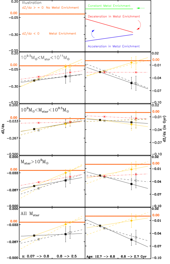
Figure 3.— Cosmic metal enrichment rate ($\frac{d\rm{Z}}{d\emph{z}}$) in two redshift (cosmic time) epochs. $\frac{d\rm{Z}}{d\emph{z}}$ is defined as the slope of the $\rm{Z}\emph{z}$ relation. Left coloumn shows $\frac{d\rm{Z}}{d\emph{z}}$ in unit of $\Delta$dex per redshift whereas the right coloumn is in unit of $\Delta$dex per Gyr. We derive $\frac{d\rm{Z}}{d\emph{z}}$ for the SDSS to the DEEP2 ($z\sim 0$ to 0.8), and the DEEP2 to the Lensed ($z\sim 0.8$ to 2.0) samples respectively (black squares/lines). As a comparison, we also derive $\frac{d\rm{Z}}{d\emph{z}}$ from $z\sim 0.8$ to 2.0 using the DEEP2 and the Erb06 samples (yellow circles/lines). Filled and empty squares are results from the mean and median quantities. The model prediction (using median) from the cosmological hydrodynamical simulation of Davé et al. (2011a) is shown in red stars. The second to fifth rows show $\frac{d\rm{Z}}{d\emph{z}}$ in different mass ranges. The first row illustrates the interpretation of the $\frac{d\rm{Z}}{d\emph{z}}$ in redshift and cosmic time frames. A negative value of $\frac{d\rm{Z}}{d\emph{z}}$ means a positive metal enrichment from high-redshift to local universe. The negative slope of $\frac{d\rm{Z}}{d\emph{z}}$ versus cosmic time (right column) indicates a deceleration in metal enrichment from from high-$z$ to low-$z$.

6. The Cosmic Evolution of Metallicity for Star-Forming Galaxies

6.1. The $\rm{Z}\emph{z}$ Relation

In this section, we present the observational investigation into the cosmic evolution of metallicity for star-forming galaxies from redshift 0 to 3. The metallicity in the local universe is represented by the SDSS sample (20577 objects, $\left<z\right>=0.072\pm 0.016$). The metallicity in the intermediate-redshift universe is represented by the DEEP2 sample (1635 objects, $\left<z\right>=0.78\pm 0.02$). For redshift $1\lesssim z\lesssim 3$, we use 19 lensed galaxies (plus 6 upper limit measurements) ($\left<z\right>=1.91\pm 0.61$) to infer the metallicity range.

The redshift distributions for the SDSS and DEEP2 samples are very narrow ($\Delta z\sim 0.02$), and the mean and median redshifts are identical within 0.001 dex. Whereas for the lensed sample, the median redshift is 2.07, and is 0.16 dex higher than the mean redshift. There are two z $\sim$ 0.9 objects in the lensed sample, and if these two objects are excluded, the mean and median redshifts for the lensed sample are $\left<z\right>=2.03\pm 0.54$, $z_{median}=2.09$ (see Table 2).

The overall metallicity distributions of the SDSS, DEEP2, and lensed samples are shown in Figure 1. Since the $z>1$ sample size is 2-3 orders of magnitude smaller than the $z<1$ samples, we use a bootstrapping process to derive the mean and median metallicities of each sample. Assuming the measured metallicity distribution of each sample is representative of their parent population, we draw from the initial sample a random subset and repeat the process for 50000 times. We use the 50000 replicated samples to measure the mean, median and standard deviations of the initial sample. This method prevents artifacts from small-number statistics and provides robust estimation of the median, mean and errors, especially for the high-$z$ lensed sample.

The fraction of low-mass (M${}_{\star}<$10⁹ M_⊙) galaxies is largest (31%) in the lensed sample, compared to 9% and 5% in the SDSS and DEEP2 samples respectively. Excluding the low-mass galaxies does not notably change the median metallicity of the SDSS and DEEP2 samples ($\sim$ 0.01 dex), while it increases the median metallicity of the lensed sample by $\sim$ 0.05 dex. To investigate whether the metallicity evolution is different for various stellar mass ranges, we separate the samples in different mass ranges and derive the mean and median metallicities (Table 2). The mass bins of 10⁹ M${}_{\odot}<$M${}_{\star}<$10^9.5 M_⊙ and 10^9.5 M${}_{\odot}<$M${}_{\star}<$10¹¹ M_⊙ are chosen such that there are similar number of lensed galaxies in each bin. Alternatively, the mass bins of 10⁹ M${}_{\odot}<$M${}_{\star}<$10¹⁰ M_⊙ and 10¹⁰ M${}_{\odot}<$M${}_{\star}<$10¹¹ M_⊙ are chosen to span equal mass scales.

We plot the metallicity ($\rm{Z}$) of all samples as a function of redshift z in Figure 2 (dubbed the $\rm{Z}\emph{z}$ plot hereafter). The first panel shows the complete observational data used in this study. The following three panels show the data and model predictions in different mass ranges. The samples at local and intermediate redshifts are large enough such that the 1$\sigma$ errors of the mean and median metallicity are smaller than the symbol sizes on the $\rm{Z}\emph{z}$ plot (0.001-0.006 dex). Although the $z>1$ samples are still composed of a relatively small number of objects, we suggest that the lensed galaxies and their bootstrapped mean and median values more closely represent the average metallicities of star-forming galaxies at $z>1$ than Lyman break, or B-band magnitude limited samples because the lensed galaxies are selected based on magnification rather than colors. Although we do note that there is still a magnitude limit and flux limit for each lensed galaxy.

We derive the metallicity evolution in units of “dex per redshift” and “dex per Gyr” using both the mean and median values. The metallicity evolution can be characterized by the slope ($\frac{d\rm{Z}}{d\emph{z}}$) of the $\rm{Z}\emph{z}$ plot. We compute $\frac{d\rm{Z}}{d\emph{z}}$ for two redshift ranges: $z\sim 0\rightarrow$ 0.8 (SDSS to DEEP2) and $z\sim 0.8\rightarrow$ $\sim$2.5 (DEEP2 to Lensed galaxies). As a comparison, we also derive $\frac{d\rm{Z}}{d\emph{z}}$ from $z\sim 0.8$ to 2.5 using the DEEP2 and the Erb06 samples (yellow circles/lines in Figure 3). We derive separate evolutions for different mass bins. We show our result in Figure 3.

A positive metallicity evolution, i.e., metals enrich galaxies from high-$z$ to the local universe, is robustly found in all mass bins from $z\sim 0.8\rightarrow$ 0. This positive evolution is indicated by the negative values of $\frac{d\rm{Z}}{d\emph{z}}$ (or $\frac{d\rm{Z}}{d\emph{z}(Gyr)}$) in Figure 3. The negative signs (both mean and median) of $\frac{d\rm{Z}}{d\emph{z}}$ are significant at $>$5 $\sigma$ of the measurement errors from $z\sim 0.8\rightarrow$ 0. From $z\sim 2.5$ to 0.8, however, $\frac{d\rm{Z}}{d\emph{z}}$ is marginally smaller than zero at the $\sim$1 $\sigma$ level from the Lensed $\rightarrow$ DEEP2 samples. If using the Erb06 $\rightarrow$ DEEP2 samples, the metallicity evolution ($\frac{d\rm{Z}}{d\emph{z}}$ ) from $z\sim 2.5$ to 0.8 is consistent with zero within $\sim$1 $\sigma$ of the measurement errors. The reason that there is no metallicity evolution from the $z\sim 2$ Erb06 $\rightarrow$ $z\sim 0.8$ DEEP2 samples may be due to the UV-selected sample of Erb06 being biased towards more metal-rich galaxies.

The right column of Figure 3 is used to interpret the deceleration/acceleration in metal enrichment. Deceleration means the metal enrichment rate ($\frac{d\rm{Z}}{d\emph{z}(Gyr)}$=$\Delta$ dex Gyr^-1) is dropping from high-$z$ to low-$z$. Using our lensed galaxies, the mean rise in metallicity is $0.055\pm 0.014$ dex Gyr^-1 for $z\sim 2.5\rightarrow 0.8$, and $0.022\pm 0.001$ dex Gyr^-1 for $z\sim 0.8\rightarrow 0$. The Mann-Whitney test shows that the mean rises in metallicity are larger for $z\sim 2.5\rightarrow 0.8$ than for $z\sim 0.8\rightarrow 0$ at a significance level of 95% for the high mass bins (10^9.5 M${}_{\odot}<$M${}_{\star}<$10¹¹ M_⊙). For lower mass bins, the hypothesis that the metal enrichment rates are the same for $z\sim 2.5\rightarrow 0.8$ and $z\sim 0.8\rightarrow 0$ can not be rejected at the 95% confidence level, i.e, there is no difference in the metal enrichment rates for the lower mass bin. Interestingly, if the Erb06 sample is used instead of the lensed sample, the hypothesis that the metal enrichment rates are the same for $z\sim 2.5\rightarrow 0.8$ and $z\sim 0.8\rightarrow 0$ can not be rejected at the 95% confidence level for all mass bins. This means that statistically, the metal enrichment rates are the same for $z\sim 2.5\rightarrow 0.8$ and $z\sim 0.8\rightarrow 0$ for all mass bins from the Erb06 $\rightarrow$ DEEP2 $\rightarrow$ SDSS samples.

The clear trend of the average/median metallicity in galaxies rising from high-redshift to the local universe is not surprising. Observations based on absorption lines have shown a continuing fall in metallicity using the damped Ly$\alpha$ absorption (DLA) galaxies at higher redshifts ($z\sim 2-5$) (e.g., Songaila & Cowie, 2002; Rafelski et al., 2012). There are several physical reasons to expect that high-$z$ galaxies are less metal-enriched: (1) high-$z$ galaxies are younger, have higher gas fractions, and have gone through less generations of star formation than local galaxies; (2) high-$z$ galaxies may be still accreting a large amount of metal-poor pristine gas from the environment, hence have lower average metallicities; (3) high-$z$ galaxies may have more powerful outflows that drive the metals out of the galaxy. It is likely that all of these mechanisms have played a role in diluting the metal content at high redshifts.

6.2. Comparison between the $\rm{Z}\emph{z}$ Relation and Theory

We compare our observations with model predictions from the cosmological hydrodynamic simulations of Davé et al. (2011a, b). These models are built within a canonical hierarchical structure formation context. The models take into account the important feedback of outflows by implementing an observation-motivated momentum-driven wind model (Oppenheimer & Davé, 2008). The effect of inflows and mergers are included in the hierarchical structure formation of the simulations. Galactic outflows are dealt specifically in the momentum-driven wind models. Davé & Oppenheimer (2007) found that the outflows are key to regulating metallicity, while inflows play a second-order regulation role.

The model of Davé et al. (2011a) focuses on the metal content of star-forming galaxies. Compared with the previous work of Davé & Oppenheimer (2007), the new simulations employ the most up-to-date treatment for supernova and AGB star enrichment, and include an improved version of the momentum-driven wind models (the $vzw$ model) where the wind properties are derived based on host galaxy masses (Oppenheimer & Davé, 2008). The model metallicity in Davé et al. (2011a) is defined as the SFR-weighted metallicity of all gas particles in the identified simulated galaxies. This model metallicity can be compared directly with the metallicity we observe in star-forming galaxies after a constant offset normalization to account for the uncertainty in the absolute metallicity scale (Kewley & Ellison, 2008). The offset is obtained by matching the model metallicity with the SDSS metallicity. Note that the model has a galaxy mass resolution limit of M${}_{\star}\sim$10⁹  M_⊙. For the $\rm{Z}\emph{z}$ plot, we normalize the model metallicity with the median SDSS metallicity computed from all SDSS galaxies $>$10⁹ M_⊙. For the MZ relation in Section 7, we normalize the model metallicity with the SDSS metallicity at the stellar mass of 10¹⁰ M_⊙.

We compute the median metallicities of the Davé et al. (2011a) model outputs in redshift bins from $z=0$ to $z=3$ with an increment of 0.1. The median metallicities with 1$\sigma$ spread (defined as including 68% of the data) of the model at each redshift are overlaid on the observational data in the $\rm{Z}\emph{z}$ plot.

We compare our observations with the model prediction in 3 ways:

(1) We compare the observed median metallicity with the model median metallicity. We see that for the lower mass bins (10^9-9.5, 10^9-10 M_⊙), the median of the model metallicity is consistent with the median of the observed metallicity within the observational errors. However, for higher mass bins, the model over-predicts the metallicity at all redshifts. The over-prediction is most significant in the highest mass bin of 10^10-11 M_⊙, where the Student’s t-statistic shows that the model distributions have significantly different means than the observational data at all redshifts, with a probability of being a chance difference of $<10^{-8}$, $<10^{-8}$, 1.7%, 5.7% for SDSS, DEEP2, the Lensed, and the Erb06 samples respectively. For the alternative high-mass bin of 10^9.5-11 M_⊙, the model also over-predicts the observed metallicity except for the Erb06 sample, with a chance difference between the model and observations of $<10^{-8}$, $<10^{-8}$, 1.7%, 8.9%, 93% for SDSS, DEEP2, the Lensed, and the Erb06 samples respectively.

(2) We compare the scatter of the observed metallicity (orange error bars on $\rm{Z}\emph{z}$ plot) with the scatter of the models (red dashed lines). For all the samples, the 1$\sigma$ scatter of the data from the SDSS ($z\sim 0$), DEEP2($z\sim 0.8$), and the Lensed sample ($z\sim 2$) are: 0.13, 0.15, and 0.15 dex; whereas the 1$\sigma$ model scatter is 0.23, 0.19, and 0.14 dex. We find that the observed metallicity scatter is increasing systematically as a function of redshift for the high mass bins whereas the model does not predict such a trend: 0.10, 0.14, 0.17 dex c.f. model 0.17, 0.15, 0.12 dex; 10^9.5-11 M_⊙ and 0.07, 0.12, 0.18 dex c.f. model 0.12, 0.11, 0.10 dex ; 10^10-11 M_⊙ from SDSS $\rightarrow$ DEEP2 $\rightarrow$ the Lensed sample. Our observed scatter is in tune with the work of Nagamine et al. (2001) in which the predicted stellar metallicity scatter increases with redshift. Note that our lensed samples are still small and have large measurement errors in metallicity ($\sim 0.2$ dex). The discrepancy between the observed scatter and models needs to be further confirmed with a larger sample.

(3) We compare the observed slope ($\frac{d\rm{Z}}{d\emph{z}}$) of the $\rm{Z}\emph{z}$ plot with the model predictions (Figure 3). We find the observed $\frac{d\rm{Z}}{d\emph{z}}$ is consistent with the model prediction within the observational errors for the undivided sample of all masses $>$10^9.0 M_⊙. However, when divided into mass bins, the model predicts a slower enrichment than observations from $z\sim 0\rightarrow 0.8$ for the lower mass bin of 10^9.0-9.5 M_⊙, and from $z\sim 0.8\rightarrow 2.5$ for the higher mass bin of 10^9.5-11 M_⊙ at a 95% significance level.

Dave et al. (2011) showed that their models over-predict the metallicities for the highest mass galaxies in the SDSS. They suggested that either (1) an additional feedback mechanism might be needed to suppress star formation in the most massive galaxies; or (2) wind recycling may be bringing in highly enriched material that elevates the galaxy metallicities. It is unclear from our data which (if any) of these interpretations is correct. Additional theoretical investigations specifically focusing on metallicities in the most massive active galaxies are needed to determine the true nature of this discrepancy.

7. Evolution of the Mass-Metallicity Relation

7.1. The Observational Limit of the Mass-Metallicity Relation

For the N2 based metallicity, there is a limiting metallicity below which the [N ii] line is too weak to be detected. Since [N ii] is the weakest of the H$\alpha$ +[N ii] lines, it is therefore the flux of [N ii] that drives the metallicity detection limit. Thus, for a given instrument sensitivity, there is a region on the mass-metallicity relation that is observationally unobtainable. Based on a few simple assumptions, we can derive the boundary of this region as follows.

Observations have shown that there is a positive correlation between the stellar mass $M_{\star}$ and $SFR$ (Noeske et al., 2007b; Elbaz et al., 2011; Wuyts et al., 2011). One explanation for the $M_{\star}$ vs. SFR relation is that more massive galaxies have earlier onset of initial star formation with shorter timescales of exponential decay (Noeske et al., 2007a; Zahid et al., 2012). The shape and amplitude of the SFR vs. $M_{\star}$ relation at different redshift $z$ can be characterized by two parameters $\delta(z)$ and $\gamma(z)$, where $\delta(z)$ is the logarithm of the SFR at $10^{10}M_{\star}$ and $\gamma(z)$ is the power law index (Zahid et al., 2012).

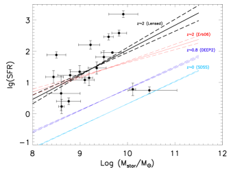
Figure 4.— SFR vs. stellar mass relation. The light-blue, blue, and red lines show the best-fit SFR vs. stellar mass relation from the SDSS, DEEP2, and Erb06 samples respectively ((Zahid et al., 2011), see also Table 3). Back dots are the lensed sample used in this work. The SFR for the lensed sample is derived from the H$\alpha$ flux with dust extinction corrected from the SED fitting. The errors on the SFR of the lensed sample are statistical errors of the H$\alpha$ fluxes. Systematic errors of the SFR can be large (a factor of 2-3) for our lensed galaxies due to complicated aperture effects (Section 3.1).

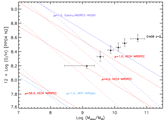
Figure 5.— The instrument detection limit on the MZ relation. We give the dependence of this detection limit in Equation 4. Shown here are examples of the detection limit based on given parameters specified as follows. The solid lines use the parameters based on the mass-SFR relation of the Erb06 sample: $\delta=1.657$ and $\gamma=0.48$ at $z=2.26$. The dashed lines use the parameters based on the mass-SFR relation of the Lensed sample: $\delta=2.02$ and $\gamma=0.69$ at $z=2.07$ (see Figure 4; Table 3). The parameters adopted for the instrument flux limit are given in Section 7.1. The lensing magnification ($\mu$) are fixed at 1.0 (i.e., non-lensing cases) for Subaru/MOIRCS (blue lines) and JWST/NIRSpec (light blue). The red lines show the detection limits for KECK/NIRSPEC with different magnifications. Black filled triangles show the Erb et al. (2006) sample. We show that stacking and/or lensing magnification can help to push the observational boundary of the MZ relation to lower mass and metallicity regions. For example, Erb et al. (2006) used stacked NIRSPEC spectra with $N\sim$ 15 spectra in each mass bin. The effect of stacking ($N\sim$ 15 per bin) is similar to observing with a lensing magnification of $\mu\sim 4$.

The relationship between the SFR and M_⋆ then becomes:

$$\log_{10}(SFR(z))=\delta(z)+\gamma(z)[\log_{10}(M_{\star}/M_{\odot})-10]$$ (1)

As an example, we show in Figure 4 the SFR vs. M_⋆ relation at three redshifts ($z\sim 0,0.8,2$). The best-fit values of $\delta(z)$ and $\gamma(z)$ are listed in Table 3.

Using the Kennicutt (1998) relation between SFR and H$\alpha$ :

$$SFR=7.9\times 10^{-42}L(H\alpha)[ergs~{}s^{-1}]$$ (2)

and the N2 metallicity calibration (Pettini & Pagel, 2004):

$$12+{\rm log(O/H)}=8.90+0.57\times{\log_{10}[NII]/H\alpha},$$ (3)

we can then derive a metallicity detection limit. We combine Equations (1), (2) and (3), and assume the [N ii]  flux is greater than the instrument flux detection limit. We provide the detection limit for the PP04N2 diagnosed MZ relation:

$$\begin{array}[]{l}\displaystyle Z_{met}\geq[\log_{10}(f_{inst}/\mu)+2\log_{10}D_{L}(z)-\gamma(z)\\ {}{}{}{}{}{}{}{}{}{}\displaystyle\\ \displaystyle~{}~{}~{}~{}~{}~{}~{}~{}~{}~{}~{}~{}~{}~{}M_{\star}-\beta(z)+\log_{10}(4\pi)]0.57+8.9\end{array}$$ (4)

where:

$$\beta(z)\equiv\delta(z)-\gamma(z)10+42-\log_{10}7.9;$$ (5)

$\delta(z)$, $\gamma(z)$ are defined in Equation (1); $f_{inst}$ is the instrument flux detection limit in $ergs~{}s^{-1}~{}cm^{-2}$; $\mu$ is the lensing magnification in flux; $D_{L}(z)$ is the luminosity distance in $cm$.

Table 3Fit to the SFR-Stellar Mass Relation

Sample	Redshift (Mean)	$\delta$	$\gamma$
SDSS	0.072	0.317$\pm$0.003	0.71 $\pm$0.01
DEEP2	0.78	0.795$\pm$0.009	0.69$\pm$0.02
Erb06	2.26	1.657$\pm$0.027	0.48$\pm$0.06
Lensed (Wuyts12)	1.69	2.93$\pm$1.28	1.47$\pm$0.14
Lensed (all)	2.07	2.02$\pm$0.83	0.69$\pm$0.09

Note. — The SFR vs. stellar mass relations at different redshifts can be characterize by two parameters $\delta(z)$ and $\gamma(z)$, where $\delta(z)$ is the logarithm of the SFR at $10^{10}M_{\star}$, and $\gamma(z)$ is the power law index. The best fits for the non-lensed samples are adopted from Zahid et al. (2012). The best fits for the lensed sample are calculated for the Wuyts et al. (2012) sample and the whole lensed sample separately.

The slope of the mass-metallicity detection limit is related to the slope of the SFR-mass relation, whereas the y-intercept of the slope depends on the instrument flux limit (and flux magnification for gravitational lensing), redshift, and the y-intercept of the SFR-mass relation.

Note that the exact location of the boundary depends on the input parameters of Equation 8. As an example, we use the $\delta(z)$ and $\gamma(z)$ values of the Erb06 and Lensed samples respectively (Table 3). We show the detection boundary for three current and future NIR instruments: Subaru/MOIRCS, KECK/NIRSPEC and JWST/NIRSpec. The instrument flux detection limit is based on background limited estimation in 10⁵ seconds (flux in units of 10^-18 ergs s^-1 cm^-2 below). For Subaru/MOIRCS (low resolution mode, HK500), we adopt $f_{inst}$ = 23.0 based on the 1$\sigma$ uncertainty of our MOIRCS spectrum (flux=4.6 in 10 hours), scaled to 3$\sigma$ in 10⁵ seconds. For KECK/NIRSPEC, we use $f_{inst}$ = 12.0, based on the 1$\sigma$ uncertainty of Erb et al. (2006) (flux=3.0 in 15 hours), scaled to 3$\sigma$ in 10⁵ seconds. For JWST/NIRSpec, we use $f_{inst}$ = 0.17, scaled to 3$\sigma$ in 10⁵ seconds.

Since lensing flux magnification is equivalent to lowering the instrument flux detection limit, we see that with a lensing magnification of $\sim$55, we reach the sensitivity of JWST using KECK/NIRSPEC. Stacking can also push the observations below the instrument flux limit. For instance, the $z\sim 2$ Erb et al. (2006) sample was obtained from stacking the NIRSPEC spectra of 87 galaxies, with $\sim$ 15 spectra in each mass bin, thus the Erb06 sample has been able to probe $\sim$ 4 times deeper than the nominal detection boundary of NIRSPEC.

The observational detection limit on the MZ relation is important for understanding the incompleteness and biases of samples due to observational constraints. However, we caution that the relation between $Z_{met}$ and M_⋆ in Equation 4 will have significant intrinsic dispersion due to variations in the observed properties of individual galaxies. This includes scatter in the M_⋆-SFR relation, the N2 metallicity calibration, the amount of dust extinction, and variable slit losses in spectroscopic observations. For example, a scatter of 0.8 dex in $\delta$ for the lensed sample (Table 3) implies a scatter of approximately 0.5 dex in $Z_{met}$. In addition, Equations 2 and 4 include implicit assumptions of zero dust extinction and no slit loss, such that the derived line flux is overestimated (and $Z_{met}$ is underestimated). Because of the above uncertainties and biases in the assumptions we made, Equation 4 should be used with due caution.

7.2. The Evolution of the MZ Relation

Figure 6 shows the mass and metallicity measured from the SDSS, DEEP2, and our lensed samples. The Erb et al. (2006) (Erb06) stacked data are also included for comparison. We highlight a few interesting features in Figure 7:

(1) To first order, the MZ relation still exists at $z\sim 2$, i.e., more massive systems are more metal rich. The Pearson correlation coefficient is $r=0.33349$, with a probability of being a chance correlation of $P=$ 17%. A simple linear fit to the lensed sample yields a slope of 0.164$\pm$0.033, with a y-intercept of 6.8$\pm$0.3.

(2) All $z>1$ samples show evidence of evolution to lower metallicities at fixed stellar masses. At high stellar mass (M${}_{\star}>$10¹⁰ M_⊙), the lensed sample has a mean metallicity and a standard deviation of the mean of 8.41$\pm$0.05, whereas the mean and standard deviation of the mean for the Erb06 sample is 8.52$\pm$0.03. The lensed sample is offset to lower metallicity by 0.11$\pm$0.06 dex compared to the Erb06 sample. This slight offset may indicate the selection difference between the UV-selected (potentially more dusty and metal rich) sample and the lensed sample (less biased towards UV bright systems).

(3) At lower mass (M${}_{\star}<$10^9.4 M_⊙), our lensed sample provides 12 individual metallicity measurements at $z>1$. The mean metallicity of the galaxies with M${}_{\star}<$10^9.4 M_⊙ is 8.25$\pm$0.05, roughly consistent with the $<$8.20 upper limit of the stacked metallicity of the lowest mass bin (M${}_{\star}\sim$10^9.1 M_⊙) of the Erb06 galaxies.

(4) Compared with the Erb06 galaxies, there is a lack of the highest mass galaxies in our lensed sample. We note that there is only 1 object with M${}_{\star}>$10^10.4 M_⊙ among all three lensed samples combined. The lensed sample is less affected by the color selection and may be more representative of the mass distribution of high-$z$ galaxies. In the hierarchical galaxy formation paradigm, galaxies grow their masses with time. The number density of massive galaxies at high redshift is smaller than at $z\sim 0$, thus the number of massive lensed galaxies is small. Selection criteria such as the UV-color selection of the Erb06 and SINs (Genzel et al., 2011) galaxies can be applied to target the high-mass galaxies on the MZ relation at high redshift.

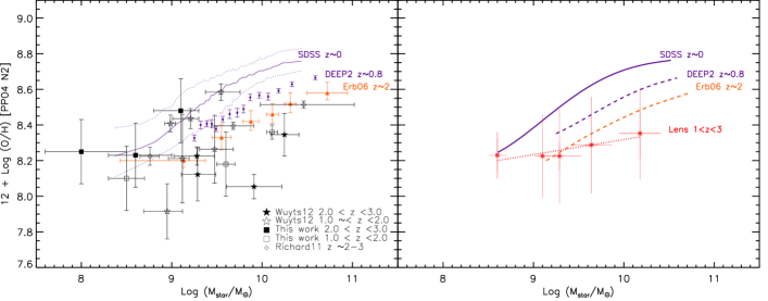
Figure 6.— Left: the observed MZ relation. Black symbols are the lensed galaxy sample at $z>1$. Specifically, the squares are from this work; the stars are from Wuyts et al. (2012), and the diamonds are from Richard et al. (2011). The orange triangles show the Erb et al. (2006) sample. The local SDSS relation and its 1-sigma range are drawn in purple lines. The $z\sim$ 0.8 DEEP2 relations from Zahid et al. (2011) are drawn in purple dots. Right: the best fit to the MZ relation. A second degree polynomial function is fit to the SDSSS, DEEEP2, and Erb06 samples. A simple linear function is fit to the lensed sample. The $z>1$ lensed data are binned in 5 mass bins (symbol: red star) and the median and 1$\sigma$ standard deviation of each bin are plotted on top of the linear fit.

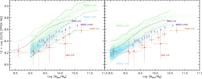
Figure 7.— Model predictions of the MZ relation. The data symbols are the same as those used in Figure 6. The small green and light blue dots are the cosmological hydrodynamic simulations with momentum-conserving wind models from Davé et al. (2011a). The difference between the left and right panels are the different normalization methods used. The left panel normalizes the model metallicity to the observed SDSS values by applying a constant offset at $M_{star}\sim 10^{10}M_{\odot}$, whereas the right panel normalizes the model metallicity to the observed SDSS metallicity by allowing a constant shift in the slope, amplitude and stellar mass. Note that the model has a mass cut off at $1.1\times 10^{9}M_{\odot}$.

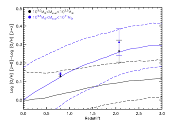
Figure 8.— The “mean evolved metallicity” as a function of redshift for two mass bins (indicated by four colors). Dashed lines show the median and 1$\sigma$ scatter of the model prediction from Davé et al. (2011a). The observed data from DEEP2 and our lensed sample are plotted as filled circles.

7.3. Comparison with Theoretical MZ Relations

Understanding the origins of the MZ relation has been the driver of copious theoretical work. Based on the idea that metallicities are mainly driven by an equilibrium among stellar enrichment, infall and outflow, Finlator & Davé (2008) developed smoothed particle hydrodynamic simulations. They found that the inclusion of a momentum-driven wind model ($vzw$) fits best to the $z\sim 2$ MZ relations compared to other outflow/wind models. The updated version of their $vzw$ model is described in detail in Davé et al. (2011a). We overlay the Davé et al. (2011a) $vzw$ model outputs on the MZ relation in Figure 7. We find that the model does not reproduce the MZ redshift evolution seen in our observations. We provide possible explanations as follows.

Kewley & Ellison (2008) found that both the shape and scatter of the MZ relation vary significantly among different metallicity diagnostics. This poses a tricky normalization problem when comparing models to observations. For example, a model output may fit the MZ relation slope from one strong-line diagnostic, but fail to fit the MZ relation from another diagnostic, which may have a very different slope. This is exactly what we are seeing on the left panel of Figure 7. Davé et al. (2011a) applied a constant offset of the model metallicities by matching the amplitude of the model MZ relation at $z\sim 0$ with the observed local MZ relation of Tremonti et al. (2004, T04) at the stellar mass of 10¹⁰ M_⊙. Davé et al. (2011a) found that the characteristic shape and scatter of the MZ relation from the $vzw$ model matches the T04 MZ relation between 10^9.0 M${}_{\odot}<$M${}_{\star}<$10^11.0 within the 1$\sigma$ model and observational scatter. However, since both the slope and amplitude of the T04 SDSS MZ relation are significantly larger than the SDSS MZ relation derived using the PP04N2 method (Kewley & Ellison, 2008), the PP04N2-normalized MZ relation from the model does not recover the local MZ relation within $1\sigma$.

In addition, the stellar mass measurements from different methods may cause a systematic offsets in the x-direction of the MZ relation (Zahid et al., 2011). As a result, even though the shape, scatter, and evolution with redshifts are independent predictions from the model, systematic uncertainties in metallicity diagnostics and stellar mass estimates do not allow the shape to be constrained separately.

In the right panel of Figure 7, we allow the model slope ($\alpha$), metallicity amplitude ($Z$), and stellar mass (M_∗) to change slightly so that it fits the local SDSS MZ relation. Assuming that this change in slope ($\Delta\alpha$), and x, y amplitudes ($\Delta Z,\Delta M_{\ast}$) are caused by the systematic offsets in observations, then the same $\Delta\alpha$, $\Delta Z$, and $\Delta M_{\ast}$ can be applied to model MZ relations at other redshifts. Although normalizing the model MZ relation in this way will make the model lose prediction power for the shape of the MZ relation, it at least leaves the redshift evolution of the MZ relation as a testable model output.

Despite the normalization correction, we see from Figure 7 that the models predict less evolution from z $\sim$ 2 to z $\sim$ 0 than the observed MZ relation. To quantify, we divide the model data into two mass bins and derive the mean and 1$\sigma$ scatter in each mass bin as a function of redshift. We define the “mean evolved metallicity” on the MZ relation as the difference between the mean metallicity at redshift $z$ and the mean metallicity at $z\sim 0$ at a fixed stellar mass (log (O/H) [z$\sim$0] $-$ log (O/H) [z$\sim$2]). The “mean evolved metallicity” errors are calculated based on the standard errors of the mean.

In Figure 8 we plot the “mean evolved metallicity” as a function of redshift for two mass bins: 10^9.0 M${}_{\odot}<$M${}_{\star}<$10^9.5 M_⊙, 10^9.5 M${}_{\odot}<$M${}_{\star}<$10¹¹ M_⊙. We calculate the observed “mean evolved metallicity” for DEEP2 and our lensed sample in the same mass bins. We see that the observed mean evolution of the lensed sample are largely uncertain and no conclusion between the model and observational data can be drawn. However, the DEEP2 data are well-constrained and can be compared with the model.

We find that at $z\sim 0.8$, the mean evolved metallicity of the high-mass galaxies are consistent with the mean evolved metallicity of the models. The observed mean evolved metallicity of the low-mass bin galaxies is $\sim$ 0.12 dex larger than the mean evolved metallicity of the models in the same mass bins.

8. Compare with Previous Work in Literature

In this Section, we compare our findings with previous work on the evolution of the MZ relation.

For low masses (10⁹ M_⊙), we find a larger enrichment (i.e., smaller decrease in metallicity) between $z\sim 2\rightarrow 0$ than either the non-lensed sample of Maiolino et al. (2008) (0.15 dex c.f. 0.6 dex) or the lensed sample of Wuyts et al. (2012); Richard et al. (2011) (0.4 dex). These discrepancies may reflect differences in metallicity calibrations applied. It is clear that a larger sample is required to characterize the true mean and spread in metallicities at intermediate redshift. Note that the lensed samples are still small and have large measurement errors in both stellar masses (0.1 to 0.5 dex) and metallicity ($\sim 0.2$ dex).

For high masses (10¹⁰ M_⊙), we find similar enrichment (0.4 dex) between $z\sim 2\rightarrow 0$ compare to the non-lensed sample of Maiolino et al. (2008) and the lensed sample of Wuyts et al. (2012); Richard et al. (2011).

We find in Section 6.1 that the deceleration in metal enrichment is significant in the highest mass bin (10^9.5 M${}_{\odot}<$M${}_{\star}<$10¹¹ M_⊙) of our samples. The deceleration in metal enrichment from $z\sim 2\rightarrow 0.8$ to $z\sim 0.8\rightarrow 0$ is consistent with the picture that the star formation and mass assembly peak between redshift 1 and 3 (Hopkins & Beacom, 2006). The deceleration is larger by 0.019$\pm$0.013 dex Gyr^-2 in the high mass bin, suggesting a possible mass-dependence in chemical enrichment, similar to the “downsizing” mass-dependent growth of stellar mass (Cowie et al., 1996; Bundy et al., 2006). In the downsizing picture, more massive galaxies formed their stars earlier and on shorter timescales compared with less massive galaxies (Noeske et al., 2007a). Our observation of the chemical downsizing is consistent with previous metallicity evolution work (Panter et al., 2008; Maiolino et al., 2008; Richard et al., 2011; Wuyts et al., 2012).

We find that for higher mass bins, the model of Davé et al. (2011a) over-predicts the metallicity at all redshifts. The over-prediction is most significant in the highest mass bin of 10^10-11 M_⊙. This conclusion similar to the findings in Davé et al. (2011a, b). In addition, we point out that when comparing the model metallicity with the observed metallicity, there is a normalization problem stemming from the discrepancy among different metallicity calibrations (Section 7.3).

We note the evolution of the MZ relation is based on an ensemble of the averaged SFR weighted metallicity of the star-forming galaxies at each epoch. The MZ relation does not reflect an evolutionary track of individual galaxies. We are probably seeing a different population of galaxies at each redshift (Brooks et al., 2007; Conroy et al., 2008). For example, a $\sim$10^10.5 M_⊙ massive galaxy at $z\sim$2 will most likely evolve into an elliptical galaxy in the local universe and will not appear on the local MZ relation. On the other hand, to trace the progenitor of a $\sim$10¹¹ M_⊙ massive galaxy today, we need to observe a $\sim$10^9.5 M_⊙ galaxy at $z\sim$2 (Zahid et al., 2012).

It is clear that gravitational lensing has the power to probe lower stellar masses than current color selection techniques. Larger lensed samples with high-quality observations are required to reduce the measurement errors.

9. Summary

To study the evolution of the overall metallicity and MZ relation as a function of redshift, it is critical to remove the systematics among different redshift samples. The major caveats in current MZ relation studies at $z>$1 are: (1) metallicity is not based on the same diagnostic method; (2) stellar mass is not derived using the same method; (3) the samples are selected differently and selection effects on mass and metallicity are poorly understood. In this paper, we attempt to minimize these issues by re-calculating the stellar mass and metallicity consistently, and by expanding the lens-selected sample at $z>$1. We aim to present a reliable observational picture of the metallicity evolution of star forming galaxies as a function of stellar mass between $0<z<3$. We find that:

• There is a clear evolution in the mean and median metallicities of star-forming galaxies as a function of redshift. The mean metallicity falls by $\sim 0.18$ dex from redshift 0 to 1 and falls further by $\sim 0.16$ dex from redshift 1 to 2.

• A more rapid evolution is seen between $z\sim 1\rightarrow 3$ than $z\sim 0\rightarrow 1$ for the high-mass galaxies (10^9.5 M${}_{\odot}<$M${}_{\star}<$10¹¹ M_⊙), with almost twice as much enrichment between $z\sim 1\rightarrow 3$ than between $z\sim 1\rightarrow 0$.

• The deceleration in metal enrichment from $z\sim 2\rightarrow 0.8$ to $z\sim 0.8\rightarrow 0$ is significant in the high-mass galaxies (10^9.5 M${}_{\odot}<$M${}_{\star}<$10¹¹ M_⊙), consistent with a mass-dependent chemical enrichment.

• We compare the metallicity evolution of star-forming galaxies from $z=0\rightarrow 3$ with the most recent cosmological hydrodynamic simulations. We see that the model metallicity is consistent with the observed metallicity within the observational error for the low mass bins. However, for higher mass bins, the model over-predicts the metallicity at all redshifts. The over-prediction is most significant in the highest mass bin of 10^10-11 M_⊙. Further theoretical investigation into the metallicity of the highest mass galaxies is required to determine the cause of this discrepancy.

• The median metallicity of the lensed sample is 0.35$\pm$0.06 dex lower than local SDSS galaxies and 0.28$\pm$0.06 dex lower than the $z\sim 0.8$ DEEP2 galaxies.

• Cosmological hydrodynamic simulation (Davé et al., 2011a) does not agree with the evolutions of the observed MZ relation based on the PP04N2 diagnostic. Whether the model fits the slope of the MZ relation depends on the normalization methods used.

This study is based on 6 clear nights of observations on a 8-meter telescope, highlighting the efficiency in using lens-selected targets. However, the lensed sample at $z>1$ is still small. We aim to significantly increase the sample size over the years.

Appendix A Slit layout, spectra for the lensed sample

This section presents the slit layouts, reduced and fitted spectra for the newly observed lensed objects in this work. The line fitting procedure is described in Section 3.2. For each target, the top panel shows the HST ACS 475W broad-band image of the lensed target. The slit layouts with different positional angles are drawn in white boxes. The bottom panel(s) show(s) the final reduced 1D spectrum(a) zoomed in for emission line vicinities. The black line is the observed spectrum for the target. The cyan line is the noise spectrum extracted from object-free pixels of the final 2D spectrum. Tilted grey mesh lines indicate spectral ranges where the sky absorption is severe. Emission lines falling in these spectral windows suffer from large uncertainties in telluric absorption correction. The blue horizontal line is the continuum fit using first order polynomial function after blanking out the severe sky absorption region. The red lines overplotted on the emission lines are the overall Gaussian fit, with the blue lines show individual components of the multiple Gaussian functions. Vertical dashed lines show the center of the Gaussian profile for each emission line. The S/N of each line are marked under the emission line labels. Note that for lines with S/N $<$3, the fit is rejected and a 3-$\sigma$ upper limit is derived.

Brief remarks on individual objects (see also Table 2 and 3 for more information):

• Figure 9 and 10, B11 (888_351) : this is a resolved galaxy with spiral-like structure at $z=2.540\pm 0.006$. As reported in Broadhurst et al. (2005), It is likely to be the most distant known spiral galaxy so far. B11 has 3 multiple images. We have observed B11.1, and B11.2, with two slit orientations on each image respectively. Different slit orientation yields very different line ratios, implying possible gradients. Our IFU follow-up observations are in progress to reveal the details of this 2.6-Gyr-old spiral.

• Figure 11 and 12, B2 (860_331): this is one of the interesting systems reported in Frye et al. (2007). It has 5 multiple images, and is only 2 $\!\!{}^{\prime\prime}$ away from another five-image lensed system, “The Sextet Arcs” at z$=$3.038. We have observed B2.1 and B2.2 and detected strong H$\alpha$ and [O iii] lines in both of them, yielding a redshift of $2.537\pm 0.006$, consistent with the redshift $z=2.534$ measured from the absorption lines ([C ii]$\,\lambda$1334, [Si ii]$\,\lambda$1527) in Frye et al. (2007).

• Figure 13, MS1 (869_328): We have detected a 7-$\sigma$ [O iii] line and determined its redshift to be $z=2.534\pm 0.010$.

• Figure 14, B29 (884_331): this is a lensed system with 5 multiple images. We observed B29.3, the brightest of the five images. The overall surface brightness of the B29.3 arc is very low, We have observed a 10-$\sigma$ H$\alpha$ and an upper limit for [N ii], placing it at $z=2.633\pm 0.010$.

• Figure 15, G3: this lensed arc with a bright knot has no recorded redshift before this study. It was put on one of the extra slits during mask designing. We have detected a 8-$\sigma$ [O iii] line and determined its redshift to be $z=2.540\pm 0.010$.

• Figure 16, Ms-Jm7 (865_359): We detected [O ii]  H$\beta$  [O iii]  H$\alpha$  and an upper limit for [N ii]  placing it at redshift $z=2.588\pm 0.006$.

• Figure 17 and 18, B5 (892_339, 870_346): it has three multiple images, of which we observed B5.1 and B5.3. Two slit orientations were observed for B5.1, the final spectrum for B5.1 has combined the two slit orientations weighted by the S/N of H$\alpha$Ṡtrong H$\alpha$ and upper limit of [N ii] were obtained in both images, yielding a redshift of $z=2.636\pm 0.004$.

• Figure 19, G2 (894_332): two slit orientations were available for G2, with detections of H$\beta$, [O iii], H$\alpha$, and upper limits for [O ii] and [N ii]. The redshift measured is $z=1.643\pm 0.010$.

• Figure 20, B12: this blue giant arc has 5 multiple images, and we observed B12.2. It shows a series of strong emission lines, with an average redshift of $z=1.834\pm 0.006$.

• Figure 21, Lensz1.36 (891_321): it has a very strong H$\alpha$ and [N ii] is at noise level, from H$\alpha$  we derive $z=1.363\pm 0.010$.

• Figure 22, MSnewz3: this is a new target observed in Abell 1689, we detect [O ii], H$\beta$, and [O iii] at a significant level, yielding $z=3.007\pm 0.003$.

• Figure 23, B8: this arc has five multiple images in total, and we observed B8.2, detection of [O ii], [O iii], H$\alpha$, with H$\beta$ and [N ii] as upper limit yields an average redshift of $z=2.662\pm 0.006$.

• B22.3: a three-image lensed system at $z=1.703\pm 0.004$, this is the first object reported from our LEGMS program, see Yuan & Kewley (2009).

• Figure 24, A68-C27: this is the only object chosen from our unfinished observations on Abell 68. This target has many strong emission lines. $z=1.762\pm 0.006$. The morphology of C27 shows signs of merger. IFU observation on this target is in process.

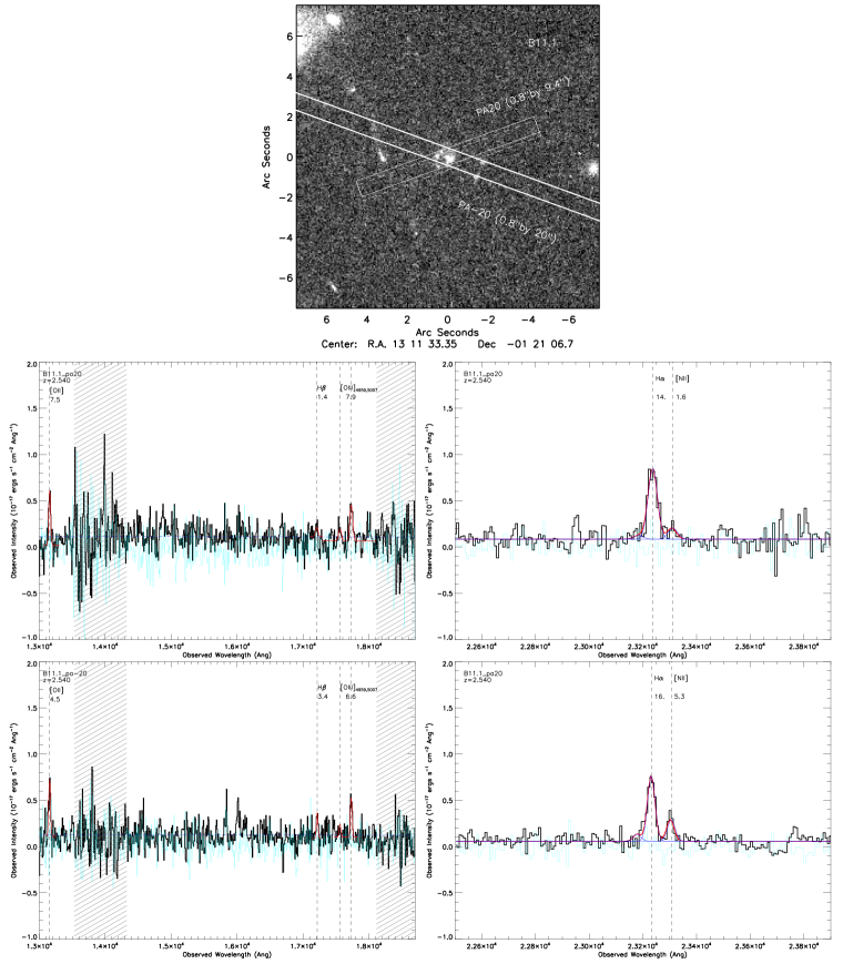
Figure 9.— z=2.540, B11.1 MOIRCS J, H band spectra. Detail descriptions are given in the Appendix text. Note that the dashed box indicates the $\sim$0.1 arcsec alignment error of MOIRCS.

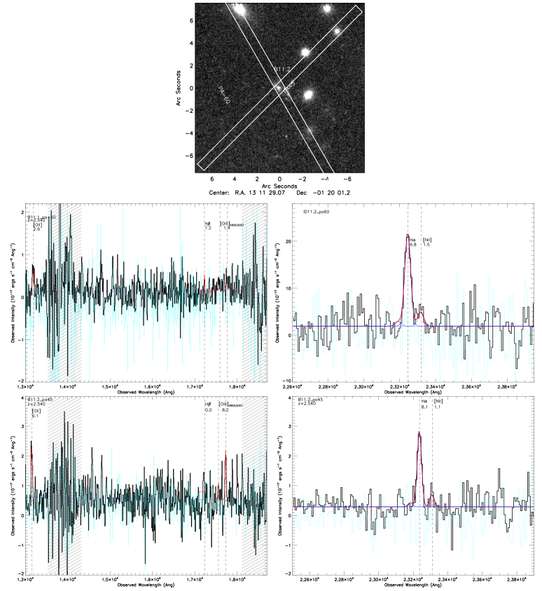
Figure 10.— z=2.540, B11.2 MOIRCS J, H band spectra. Detail descriptions are given in the Appendix text.

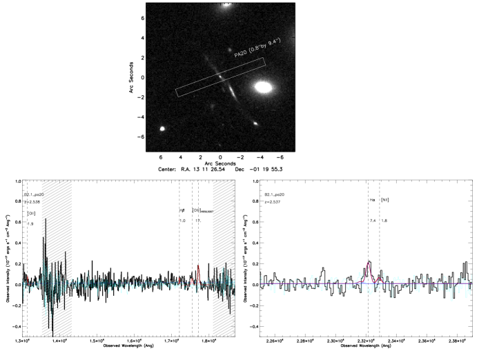
Figure 11.— z=2.537, B2.1, MOIRCS J, H band spectra. Detail descriptions are given in the Appendix text.

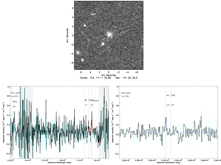
Figure 12.— z=2.537, B2.2, MOIRCS J, H band spectra. Detail descriptions are given in the Appendix text.

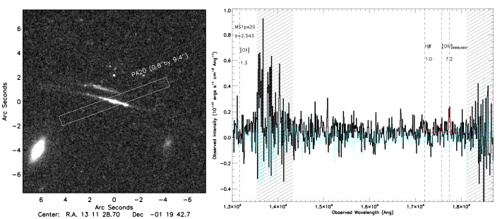
Figure 13.— z=2.54, MS1, MOIRCS J, H band spectra. Detail descriptions are given in the Appendix text.

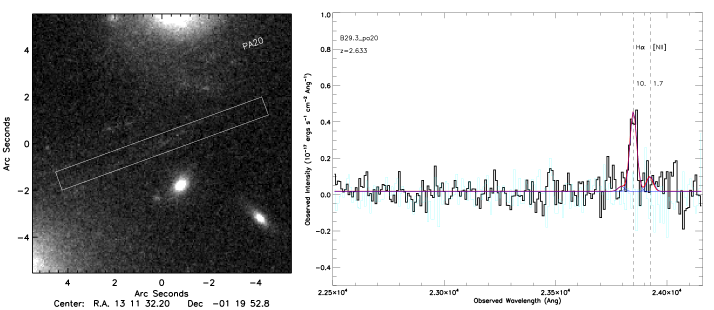
Figure 14.— z=2.633, B29.3, MOIRCS J, H band spectra. Detail descriptions are given in the Appendix text.

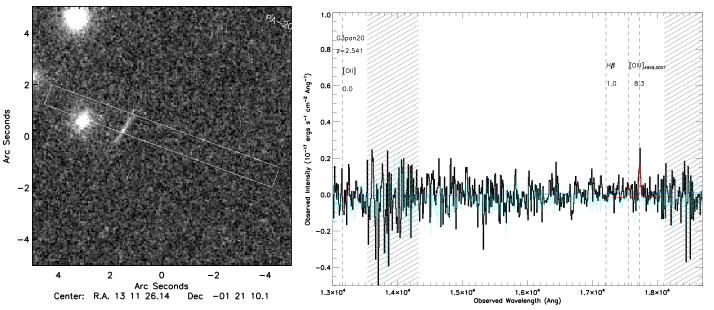
Figure 15.— z=2.540, G3, MOIRCS J, H band spectra. Detail descriptions are given in the Appendix text.

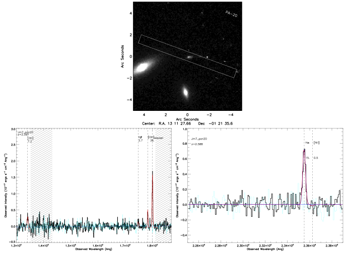
Figure 16.— z=2.588, Jm7, MOIRCS J, H band spectra. Detail descriptions are given in the Appendix text.

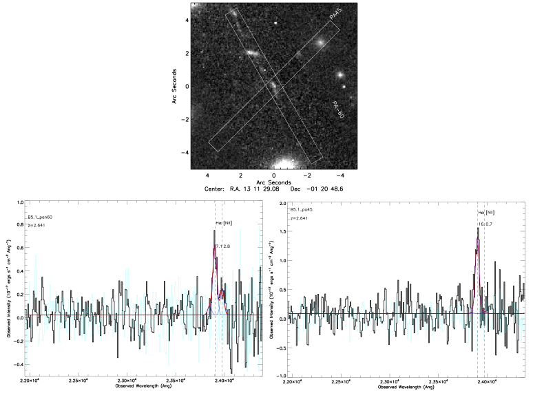
Figure 17.— z=2.641, B5.1, MOIRCS J, H band spectra. Note that the reason that the flux of B5.1 in slit position PAn60 is less than PA45 (B5.1+B5.2) is that the dithering length of PAn60 was smaller than the separation of 5.1 and 5.2, thus part of the flux of PA45 (B5.1+B5.2) was cancelled out during the dithering process. Detail descriptions are given in the Appendix text.

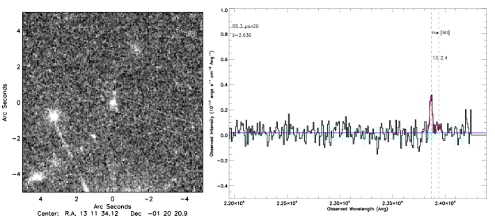
Figure 18.— z=2.636, B5.3, MOIRCS J, H band spectra. Detail descriptions are given in the Appendix text.

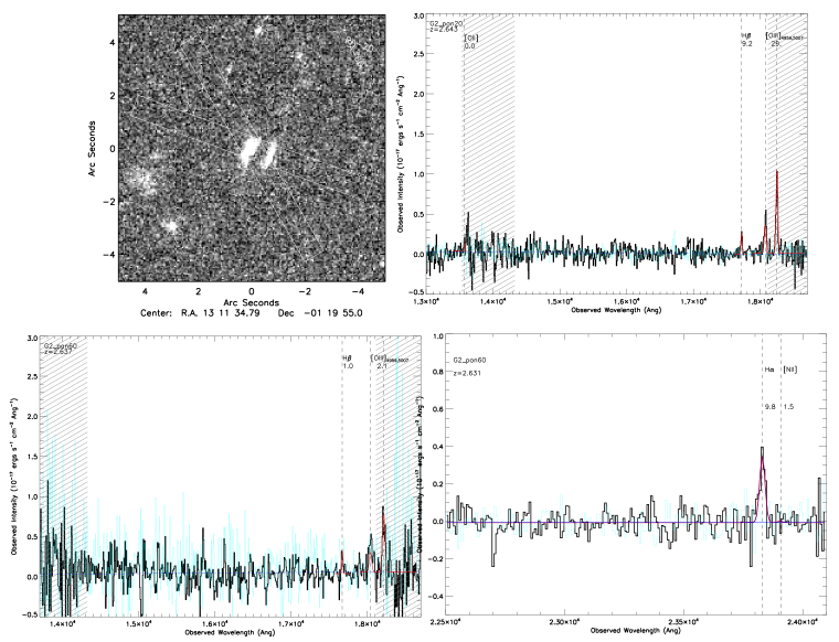
Figure 19.— z=2.643, G2, MOIRCS J, H band spectra. Detail descriptions are given in the Appendix text.

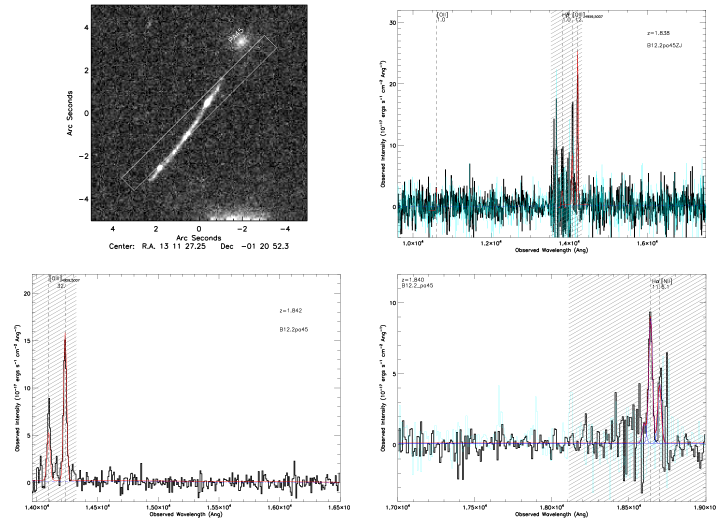
Figure 20.— z=1.834$\pm$0.002, B12.2, MOIRCS J, H band spectra. Detail descriptions are given in the Appendix text.

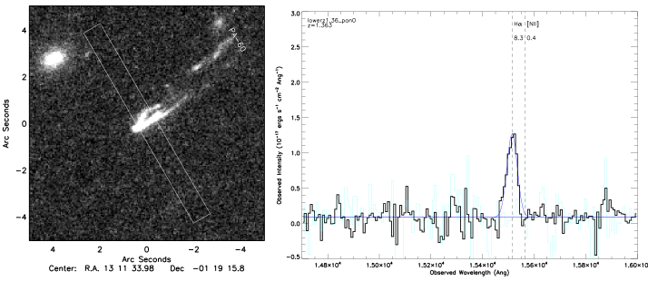
Figure 21.— z=1.363, Low-z, MOIRCS J, H band spectra. Detail descriptions are given in the Appendix text.

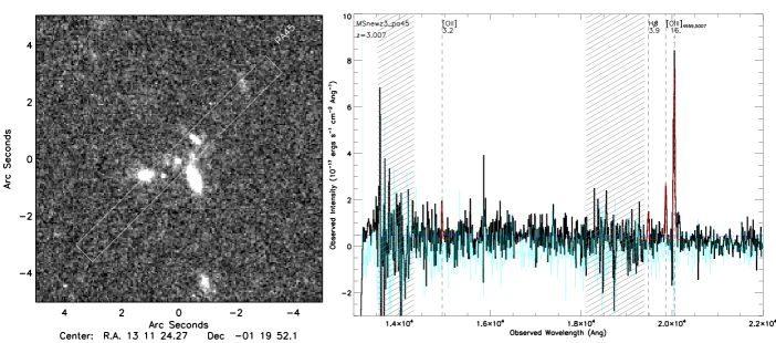
Figure 22.— z=3.003, new target, MOIRCS J, H band spectra. Detail descriptions are given in the Appendix text.

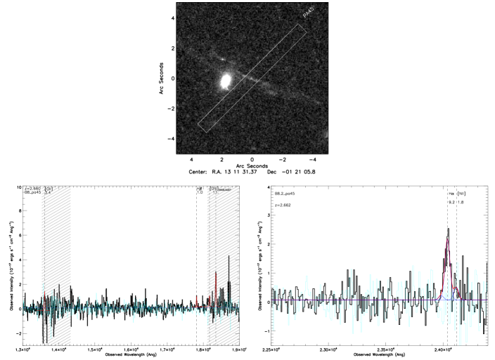
Figure 23.— z=2.663, B8.2, MOIRCS J, H band spectra. Detail descriptions are given in the Appendix text.

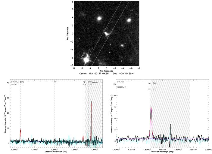
Figure 24.— z=1.763, A68C27, MOIRCS J, H band spectra. Detail descriptions are given in the Appendix text.

Table 4Measured Emission Line fluxes

Id	[O ii]$\,\lambda$3727	H$\beta$	[O iii]$\,\lambda$5007	H$\alpha$	[N ii]$\,\lambda$6584	KK04($\to$PP04N2)	Branch	PP04N2	E(B-V)	Final Adopted
B11.1:pa20	21.43$\pm$2.60	5.42$\pm$1.63	21.12$\pm$2.43	33.54$\pm$2.38	$<$4.59	8.38(8.16)$\pm$0.14	up	$<$8.41	0.73$\pm$0.29	8.48$\pm$0.18
B11.1:pa-20	22.02$\pm$4.88	9.40$\pm$2.75	14.78$\pm$2.21	28.13$\pm$2.56	8.90$\pm$0.89	8.74(8.54)$\pm$0.14	up	8.61$\pm$0.05	0.05$\pm$0.29
B11.2:pa-60	$<$60.5	$<$64.6	$<$60.3	53.6$\pm$4.09	$<$17.12	$\cdots$	$\cdots$	$<$8.62	$\cdots$
B11.2:pa45	73.65$\pm$12.01	$<$34.23	61.06$\pm$7.4	80.46$\pm$9.9	$<$13.08	$<$8.74(8.54)	up	$<$8.73	0.
B2.1:pa20	$<$2.82	$<$6.3	9.47$\pm$0.56	7.66$\pm$0.69	$<$0.67	$\cdots$	$\cdots$	$<$8.30	$\cdots$	$<$8.30
B2.2:pa20	$<$7.73	$<$20.6	23.2$\pm$3.0	$<$5.45	$<$6.4	$\cdots$	$\cdots$	$\cdots$	$\cdots$	$\cdots$
MS1:pa20	$<3.08$	$<$4.5	6.7$\pm$0.9	$\cdots$	$\cdots$	$\cdots$	$\cdots$	$\cdots$	$\cdots$	$\cdots$
B29.3:pa20	$\cdots$	$\cdots$	$\cdots$	17.05$\pm$1.6	$<$3.1	$\cdots$	$\cdots$	$<$8.48	$\cdots$	$<$8.48
G3:pan20	$\cdots$	$<$4.0	6.0$\pm$0.7	$\cdots$	$\cdots$	$\cdots$	$\cdots$	$\cdots$	$\cdots$	$\cdots$
MS-Jm7:pan20	19.16$\pm$2.74	12.5$\pm$3.6	58.12$\pm$1.64	23.03$\pm$1.6	$<$9.22	8.69(8.33)$\pm$0.12	up	$<$8.67	0.	8.25$\pm$0.18
						8.23(8.19)$\pm$0.12	low
B5.3:pan20	$\cdots$	$\cdots$	$\cdots$	9.07$\pm$0.7	$<$2.94	$\cdots$	$\cdots$	$<$8.62	$\cdots$	$<$8.62
B5.1:pan20	$\cdots$	$\cdots$	$\cdots$	30.38$\pm$4.6	$<$13.34	$\cdots$	$\cdots$	$<$8.70	$\cdots$
B5.1:pa45	$\cdots$	$\cdots$	$\cdots$	64.39$\pm$3.9	$<$59.5	$\cdots$	$\cdots$	$<$8.88	$\cdots$
G2:pan20	$<$4.7	6.84$\pm$0.74	36.49$\pm$1.25	$\cdots$	$\cdots$	$<$8.62(8.41)	up	$\cdots$	$\cdots$	$<$8.41
G2:pan60	$<$25.8	$<$8.8	$<$98.7	10.09$\pm$1.0	$<$3.1	$\cdots$	$\cdots$	$<$8.60	$\cdots$
Lowz1.36:pan60	$\cdots$	$\cdots$	$\cdots$	59.19$\pm$7.1	$<$8.82	$\cdots$	$\cdots$	$<$8.43	$\cdots$	$<$8.43
MSnewz3:pa45	36.94$\pm$11.5	44.02$\pm$11.06	300.3$\pm$17.8	$\cdots$	$\cdots$	8.5(8.29)$\pm$0.11	up	$\cdots$	$\cdots$	8.23$\pm$0.18
						8.12(8.16)$\pm$0.11	low	$\cdots$	$\cdots$
B12.2:pa45	$<$71.58	$<67.79$	141.01$\pm$10.07	90.45$\pm$6.95	$<10.6$	$\cdots$	$\cdots$	$<$8.369	$\cdots$	$<$8.369
B8.2:pa45	40.2$\pm$11.8	$<$17.7	75.7$\pm$6.6	115.26$\pm$12.5	$<$72.13	$<$8.51(8.29)	up	$<$8.78	$>$1.2	$<$8.29
						$<$8.11(8.16)	low	$\cdots$	$\cdots$
B22.3:pa60	162.1$\pm$20.3	146.0$\pm$29.2	942.3$\pm$62.8	734.4$\pm$56.5	$<$3.65	8.13(8.17)$\pm$0.12	low	$<$8.22	0.54$\pm$0.22	8.10$\pm$0.18
A68-C27:pa60	317.01$\pm$17.9	149.2$\pm$17.5	884.4$\pm$58.9	814.6$\pm$21.8	40.4$\pm$10.92	8.26(8.25)$\pm$0.06	low	8.16$\pm$0.07	0.62$\pm$0.11	8.16$\pm$0.18

Note. — Observed emission line fluxes for the lensed background galaxies in A1689. Fluxes are in units of 10^-17 ergs s^-1 cm^-2, without lensing magnification correction. Some lines are not detected because of the severe telluric absorption.

Table 5Physical Properties of the Lensed Sample

ID1	ID2	RA, DEC (J2000)	Redshift	lg(SFR)	Lensing Magnification	log(M∗/M⊙)
				(M⊙ yr-1)	(flux)
B11.1:pa20	888_351	13:11:33.336, -01:21:06.94	2.540$\pm$0.006	1.08$\pm$0.1	11.8$\pm$2.7	9.1${}^{+0.2}_{-0.3}$
B11.2:pa45	$\cdots$	13:11:29.053, -01:20:01.26	2.540$\pm$0.006	1.42$\pm$0.11	13.1$\pm$1.8
B2.1:pa20	860_331	13:11:26.521, -01:19:55.24	2.537$\pm$0.006	0.20$\pm$0.03	20.6$\pm$1.8	8.2${}^{+0.3}_{-0.3}$
B2.2:pa20	$\cdots$	13:11:32.961, -01:20:25.31	2.537$\pm$0.006	$\cdots$	15.0$\pm$2.0
MS1:pa20	869_328	13:11:28.684,-01:19:42.62	2.534$\pm$0.01	$\cdots$	58.3$\pm$2.8	8.5${}^{+0.1}_{-0.1}$
B29.3:pa20	884_331	13:11:32.164,-01:19:52.53	2.633$\pm$0.01	0.43$\pm$0.06	22.5$\pm$6.9	9.0${}^{+0.4}_{-0.5}$
G3:pan20	$\cdots$	13:11:26.219,-01:21:09.64	2.540$\pm$0.01	$\cdots$	7.7$\pm$0.1	$\cdots$
MS-Jm7:pan20	865_359	13:11:27.600,-01:21:35.00	2.588$\pm$0.006	$\cdots$	18.5$\pm$3.2	8.0${}^{+0.5}_{-0.4}$
B5.3:pan20	892_339	13:11:34.109,-01:20:20.90	2.636$\pm$0.004	0.47$\pm$0.05	14.2$\pm$1.3	9.1${}^{+0.4}_{-0.2}$
B5.1:pan60	870_346	13:11:29.064,-01:20:48.33	2.641$\pm$0.004	1.0$\pm$0.05	14.3$\pm$0.3
G2	894_332	13:11:34.730,-01:19:55.53	1.643$\pm$0.01	0.45$\pm$0.09	16.7$\pm$3.1	8.0${}^{+0.3}_{-0.4}$
Lowz1.36	891_321	13:11:33.957,-01:19:15.90	1.363$\pm$0.01	0.67$\pm$0.11	11.6$\pm$2.7	8.9${}^{+0.3}_{-0.3}$
MSnewz3:pa45	$\cdots$	13:11:24.276,-01:19:52.08	3.007$\pm$0.003	0.65$\pm$0.55	2.9$\pm$1.7	8.6${}^{+0.3}_{-0.4}$
B12.2:pa45	863_348	13:11:27.212,-01:20:51.89	1.834$\pm$0.006	1.00$\pm$0.05	56.0$\pm$4.4	7.4${}^{+0.2}_{-0.0}$
B8.2:pa45	$\cdots$	13:11:27.212,-01:20:51.89	2.662$\pm$0.006	1.36$\pm$0.07	23.7$\pm$3.0	8.2${}^{+0.5}_{-0.6}$
B22.3:pa60	$\cdots$	13:11:32.4150,-01:21:15.917	1.703$\pm$0.006	1.88$\pm$0.04	15.5$\pm$0.3	8.5${}^{+0.2}_{-0.2}$
A68-C27:pa60	$\cdots$	00:37:04.866,+09:10:29.26	1.762$\pm$0.006	2.46$\pm$0.1	4.9$\pm$1.1	9.6${}^{+0.1}_{-0.1}$

Note. — The redshift errors in Table 5 is determined from RMS of different emission line centroids. If the RMS is smaller than 0.006 (for most targets) or if there is only one line fitted, we adopt the systematic error of 0.006 as a conservative estimation for absolute redshift measurements.

References

- Abazajian et al. (2009) Abazajian, K. N., et al. 2009, ApJS, 182, 543
- Asplund et al. (2009) Asplund, M., Grevesse, N., Sauval, A. J., & Scott, P. 2009, ARA&A, 47, 481
- Baldwin et al. (1981) Baldwin, J. A., Phillips, M. M., & Terlevich, R. 1981, PASP, 93, 5
- Bertin & Arnouts (1996) Bertin, E., & Arnouts, S. 1996, A&AS, 117, 393
- Bertone et al. (2007) Bertone, S., De Lucia, G., & Thomas, P. A. 2007, MNRAS, 379, 1143
- Brinchmann et al. (2008) Brinchmann, J., Pettini, M., & Charlot, S. 2008, MNRAS, 385, 769
- Broadhurst et al. (2005) Broadhurst, T., et al. 2005, ApJ, 621, 53
- Brooks et al. (2007) Brooks, A. M., Governato, F., Booth, C. M., Willman, B., Gardner, J. P., Wadsley, J., Stinson, G., & Quinn, T. 2007, ApJ, 655, L17
- Bruzual & Charlot (2003) Bruzual, G., & Charlot, S. 2003, MNRAS, 344, 1000
- Bundy et al. (2006) Bundy, K., et al. 2006, ApJ, 651, 120
- Calzetti et al. (2000) Calzetti, D., Armus, L., Bohlin, R. C., Kinney, A. L., Koornneef, J., & Storchi-Bergmann, T. 2000, ApJ, 533, 682
- Capak et al. (2004) Capak, P., et al. 2004, AJ, 127, 180
- Chabrier (2003) Chabrier, G. 2003, PASP, 115, 763
- Chapman et al. (2005) Chapman, S. C., Blain, A. W., Smail, I., & Ivison, R. J. 2005, ApJ, 622, 772
- Christensen et al. (2012) Christensen, L., et al. 2012, ArXiv e-prints
- Conroy et al. (2008) Conroy, C., Shapley, A. E., Tinker, J. L., Santos, M. R., & Lemson, G. 2008, ApJ, 679, 1192
- Conselice et al. (2007) Conselice, C. J., et al. 2007, MNRAS, 381, 962
- Cowie & Barger (2008) Cowie, L. L., & Barger, A. J. 2008, ApJ, 686, 72
- Cowie et al. (1996) Cowie, L. L., Songaila, A., Hu, E. M., & Cohen, J. G. 1996, AJ, 112, 839
- Daddi et al. (2004) Daddi, E., Cimatti, A., Renzini, A., Fontana, A., Mignoli, M., Pozzetti, L., Tozzi, P., & Zamorani, G. 2004, ApJ, 617, 746
- Dalcanton (2007) Dalcanton, J. J. 2007, ApJ, 658, 941
- Davé et al. (2011a) Davé, R., Finlator, K., & Oppenheimer, B. D. 2011a, MNRAS, 416, 1354
- Davé & Oppenheimer (2007) Davé, R., & Oppenheimer, B. D. 2007, MNRAS, 374, 427
- Davé et al. (2011b) Davé, R., Oppenheimer, B. D., & Finlator, K. 2011b, MNRAS, 415, 11
- Davies (2007) Davies, R. I. 2007, MNRAS, 375, 1099
- Davis et al. (2003) Davis, M., et al. 2003, in Society of Photo-Optical Instrumentation Engineers (SPIE) Conference Series, Vol. 4834, Society of Photo-Optical Instrumentation Engineers (SPIE) Conference Series, ed. P. Guhathakurta, 161–172
- De Lucia et al. (2004) De Lucia, G., Kauffmann, G., & White, S. D. M. 2004, MNRAS, 349, 1101
- Dickinson et al. (2003) Dickinson, M., Papovich, C., Ferguson, H. C., & Budavári, T. 2003, ApJ, 587, 25
- Edmunds (1990) Edmunds, M. G. 1990, MNRAS, 246, 678
- Edmunds & Greenhow (1995) Edmunds, M. G., & Greenhow, R. M. 1995, MNRAS, 272, 241
- Elbaz et al. (2011) Elbaz, D., et al. 2011, A&A, 533, A119
- Erb et al. (2010) Erb, D. K., Pettini, M., Shapley, A. E., Steidel, C. C., Law, D. R., & Reddy, N. A. 2010, ApJ, 719, 1168
- Erb et al. (2006) Erb, D. K., Shapley, A. E., Pettini, M., Steidel, C. C., Reddy, N. A., & Adelberger, K. L. 2006, ApJ, 644, 813
- Erb et al. (2003) Erb, D. K., Shapley, A. E., Steidel, C. C., Pettini, M., Adelberger, K. L., Hunt, M. P., Moorwood, A. F. M., & Cuby, J.-G. 2003, ApJ, 591, 101
- Fan et al. (2001) Fan, X., et al. 2001, AJ, 121, 54
- Finlator & Davé (2008) Finlator, K., & Davé, R. 2008, MNRAS, 385, 2181
- Förster Schreiber et al. (2006) Förster Schreiber, N. M., et al. 2006, ApJ, 645, 1062
- Förster Schreiber et al. (2011) Förster Schreiber, N. M., Shapley, A. E., Erb, D. K., Genzel, R., Steidel, C. C., Bouché, N., Cresci, G., & Davies, R. 2011, ApJ, 731, 65
- Frye et al. (2007) Frye, B. L., et al. 2007, ApJ, 665, 921
- Garnett (2002) Garnett, D. R. 2002, ApJ, 581, 1019
- Genzel et al. (2008) Genzel, R., et al. 2008, ApJ, 687, 59
- Genzel et al. (2011) —. 2011, ApJ, 733, 101
- Grazian et al. (2007) Grazian, A., et al. 2007, A&A, 465, 393
- Hayashi et al. (2009) Hayashi, M., et al. 2009, ApJ, 691, 140
- Henry et al. (2010) Henry, J. P., et al. 2010, ApJ, 725, 615
- Hopkins & Beacom (2006) Hopkins, A. M., & Beacom, J. F. 2006, ApJ, 651, 142
- Ichikawa et al. (2006) Ichikawa, T., et al. 2006, in Society of Photo-Optical Instrumentation Engineers (SPIE) Conference Series, Vol. 6269
- Ilbert et al. (2009) Ilbert, O., et al. 2009, ArXiv e-prints
- Jones et al. (2010) Jones, T., Ellis, R., Jullo, E., & Richard, J. 2010, ApJ, 725, L176
- Jones et al. (2012) Jones, T., Ellis, R. S., Richard, J., & Jullo, E. 2012, ArXiv e-prints
- Jullo et al. (2007) Jullo, E., Kneib, J.-P., Limousin, M., Elíasdóttir, Á., Marshall, P. J., & Verdugo, T. 2007, New Journal of Physics, 9, 447
- Kelson (2003) Kelson, D. D. 2003, PASP, 115, 688
- Kennicutt (1998) Kennicutt, Jr., R. C. 1998, ARA&A, 36, 189
- Kewley & Dopita (2002) Kewley, L. J., & Dopita, M. A. 2002, ApJS, 142, 35
- Kewley & Ellison (2008) Kewley, L. J., & Ellison, S. L. 2008, ApJ, 681, 1183
- Kewley et al. (2004) Kewley, L. J., Geller, M. J., & Jansen, R. A. 2004, AJ, 127, 2002
- Kewley et al. (2006) Kewley, L. J., Groves, B., Kauffmann, G., & Heckman, T. 2006, MNRAS, 372, 961
- Kneib et al. (1993) Kneib, J. P., Mellier, Y., Fort, B., & Mathez, G. 1993, A&A, 273, 367
- Kobulnicky & Kewley (2004) Kobulnicky, H. A., & Kewley, L. J. 2004, ApJ, 617, 240
- Köppen & Edmunds (1999) Köppen, J., & Edmunds, M. G. 1999, MNRAS, 306, 317
- Kriek et al. (2007) Kriek, M., et al. 2007, ApJ, 669, 776
- Lacey & Fall (1985) Lacey, C. G., & Fall, S. M. 1985, ApJ, 290, 154
- Lamareille et al. (2009) Lamareille, F., et al. 2009, A&A, 495, 53
- Lara-Lopez et al. (2012) Lara-Lopez, M. A., Lopez-Sanchez, A. R., & Hopkins, A. M. 2012, ArXiv e-prints
- Larkin et al. (2006) Larkin, J., et al. 2006, New Astronomy Reviews, 50, 362
- Law et al. (2009) Law, D. R., Steidel, C. C., Erb, D. K., Larkin, J. E., Pettini, M., Shapley, A. E., & Wright, S. A. 2009, ApJ, 697, 2057
- Lemoine-Busserolle et al. (2003) Lemoine-Busserolle, M., Contini, T., Pelló, R., Le Borgne, J.-F., Kneib, J.-P., & Lidman, C. 2003, A&A, 397, 839
- Lequeux et al. (1979) Lequeux, J., Peimbert, M., Rayo, J. F., Serrano, A., & Torres-Peimbert, S. 1979, A&A, 80, 155
- Limousin et al. (2007) Limousin, M., et al. 2007, ApJ, 668, 643
- Liu et al. (2008) Liu, X., Shapley, A. E., Coil, A. L., Brinchmann, J., & Ma, C.-P. 2008, ApJ, 678, 758
- Maiolino et al. (2008) Maiolino, R., et al. 2008, A&A, 488, 463
- Mannucci et al. (2010) Mannucci, F., Cresci, G., Maiolino, R., Marconi, A., & Gnerucci, A. 2010, MNRAS, 408, 2115
- McLean et al. (1998) McLean, I. S., et al. 1998, in Presented at the Society of Photo-Optical Instrumentation Engineers (SPIE) Conference, Vol. 3354, Society of Photo-Optical Instrumentation Engineers (SPIE) Conference Series, ed. A. M. Fowler, 566–578
- Nagamine et al. (2001) Nagamine, K., Fukugita, M., Cen, R., & Ostriker, J. P. 2001, ApJ, 558, 497
- Noeske et al. (2007a) Noeske, K. G., et al. 2007a, ApJ, 660, L47
- Noeske et al. (2007b) —. 2007b, ApJ, 660, L43
- Oke et al. (1995) Oke, J. B., et al. 1995, PASP, 107, 375
- Oppenheimer & Davé (2008) Oppenheimer, B. D., & Davé, R. 2008, MNRAS, 387, 577
- Osterbrock (1989) Osterbrock, D. E. 1989, Astrophysics of gaseous nebulae and active galactic nuclei (Research supported by the University of California, John Simon Guggenheim Memorial Foundation, University of Minnesota, et al. Mill Valley, CA, University Science Books, 1989, 422 p.)
- Pagel & Edmunds (1981) Pagel, B. E. J., & Edmunds, M. G. 1981, ARA&A, 19, 77
- Pagel & Patchett (1975) Pagel, B. E. J., & Patchett, B. E. 1975, MNRAS, 172, 13
- Panter et al. (2008) Panter, B., Jimenez, R., Heavens, A. F., & Charlot, S. 2008, MNRAS, 391, 1117
- Pettini & Pagel (2004) Pettini, M., & Pagel, B. E. J. 2004, MNRAS, 348, L59
- Pettini et al. (2001) Pettini, M., Shapley, A. E., Steidel, C. C., Cuby, J.-G., Dickinson, M., Moorwood, A. F. M., Adelberger, K. L., & Giavalisco, M. 2001, ApJ, 554, 981
- Quider et al. (2009) Quider, A. M., Pettini, M., Shapley, A. E., & Steidel, C. C. 2009, MNRAS, 1081
- Rafelski et al. (2012) Rafelski, M., Wolfe, A. M., Prochaska, J. X., Neeleman, M., & Mendez, A. J. 2012, ApJ, 755, 89
- Reddy et al. (2006) Reddy, N. A., Steidel, C. C., Erb, D. K., Shapley, A. E., & Pettini, M. 2006, ApJ, 653, 1004
- Reddy et al. (2008) Reddy, N. A., Steidel, C. C., Pettini, M., Adelberger, K. L., Shapley, A. E., Erb, D. K., & Dickinson, M. 2008, ApJS, 175, 48
- Richard et al. (2011) Richard, J., Jones, T., Ellis, R., Stark, D. P., Livermore, R., & Swinbank, M. 2011, MNRAS, 126
- Richard et al. (2007) Richard, J., et al. 2007, ApJ, 662, 781
- Rubin et al. (1984) Rubin, V. C., Ford, Jr., W. K., & Whitmore, B. C. 1984, ApJ, 281, L21
- Savaglio et al. (2005) Savaglio, S., et al. 2005, ApJ, 635, 260
- Searle & Sargent (1972) Searle, L., & Sargent, W. L. W. 1972, ApJ, 173, 25
- Shapley et al. (2005) Shapley, A. E., Coil, A. L., Ma, C.-P., & Bundy, K. 2005, ApJ, 635, 1006
- Skillman et al. (1989) Skillman, E. D., Kennicutt, R. C., & Hodge, P. W. 1989, ApJ, 347, 875
- Sobral et al. (2009) Sobral, D., et al. 2009, MNRAS, 398, 75
- Songaila & Cowie (2002) Songaila, A., & Cowie, L. L. 2002, AJ, 123, 2183
- Stark et al. (2008) Stark, D. P., Swinbank, A. M., Ellis, R. S., Dye, S., Smail, I. R., & Richard, J. 2008, Nature, 455, 775
- Steidel et al. (2003) Steidel, C. C., Adelberger, K. L., Shapley, A. E., Pettini, M., Dickinson, M., & Giavalisco, M. 2003, ApJ, 592, 728
- Steidel et al. (1996) Steidel, C. C., Giavalisco, M., Pettini, M., Dickinson, M., & Adelberger, K. L. 1996, ApJ, 462, L17
- Steidel et al. (2004) Steidel, C. C., Shapley, A. E., Pettini, M., Adelberger, K. L., Erb, D. K., Reddy, N. A., & Hunt, M. P. 2004, ApJ, 604, 534
- Swinbank et al. (2009) Swinbank, A. M., et al. 2009, MNRAS, 400, 1121
- Tremonti et al. (2004) Tremonti, C. A., et al. 2004, ApJ, 613, 898
- Veilleux & Osterbrock (1987) Veilleux, S., & Osterbrock, D. E. 1987, ApJS, 63, 295
- Wuyts et al. (2012) Wuyts, E., Rigby, J. R., Sharon, K., & Gladders, M. D. 2012, ApJ, 755, 73
- Wuyts et al. (2011) Wuyts, S., et al. 2011, ApJ, 742, 96
- Yabe et al. (2012) Yabe, K., et al. 2012, PASJ, 64, 60
- Yates et al. (2012) Yates, R. M., Kauffmann, G., & Guo, Q. 2012, MNRAS, 422, 215
- Yuan & Kewley (2009) Yuan, T.-T., & Kewley, L. J. 2009, ApJ, 699, L161
- Yuan et al. (2011) Yuan, T.-T., Kewley, L. J., Swinbank, A. M., Richard, J., & Livermore, R. C. 2011, ApJ, 732, L14+
- Zahid et al. (2012) Zahid, H. J., Dima, G. I., Kewley, L. J., Erb, D. K., & Dave, R. 2012, ArXiv e-prints
- Zahid et al. (2011) Zahid, H. J., Kewley, L. J., & Bresolin, F. 2011, ApJ, 730, 137
- Zaritsky et al. (1994) Zaritsky, D., Kennicutt, Jr., R. C., & Huchra, J. P. 1994, ApJ, 420, 87