Constraining dark matter sub-structure with the dynamics of astrophysical systems

Abstract

The accuracy of the measurements of some astrophysical dynamical systems allows to constrain the existence of incredibly small gravitational perturbations. In particular, the internal Solar System dynamics (planets, Earth-Moon) opens up the possibility, for the first time, to prove the abundance, mass and size, of dark sub-structures at the Earth vicinity. We find that adopting the standard dark matter density, its local distribution can be composed by sub-solar mass halos with no currently measurable dynamical consequences, regardless of the mini-halo fraction. On the other hand, it is possible to exclude the presence of dark streams with linear mass densities higher than $\lambda_{\rm st}>10^{-10}\textrm{M}_{\astrosun}/\textrm{AU}$ (about the Earth mass spread along the diameter of the SS up to the Kuiper belt). In addition, we review the dynamics of wide binaries inside the dwarf spheroidal galaxies in the Milky Way. The dynamics of such kind of binaries seem to be compatible with the presence of a huge fraction of dark sub-structure, thus their existence is not a sharp discriminant of the dark matter hypothesis as been claimed before. However, there are regimes where the constraints from different astrophysical systems may reveal the sub-structure mass function cut-off scale.

1 Introduction

The $\Lambda-\textrm{C$\textrm{DM}$}$ cosmological model assumes the existence of two unknown energy components; a cosmological constant, $\Lambda$, and the Cold Dark Matter, CDM. This model is the paradigm on cosmology due to the high precision at which the observations of the large scale Universe are described (Cosmic Microwave Background radiation [1], large surveys of galaxies [2], gravitational lensing surveys [3], etc.). Such observations seem to be equally satisfied independently of the dark matter, (DM), nature; although it has to be quite cold (low velocities) [4], it can have a small self-interaction [5], and at most a weak interaction with the standard model of particles [6, 7].  On the other hand, observations at sub-galactic scales are sensitive to the particle physics of the DM.

In the current paradigm structure grows from bottom up; the first objects formed at high redshift were some small sub-galactic units that collapsed from small perturbations in the primordial density field [14]. These clumps then merge hierarchically to form the large bound objects we observe in the local universe today. The properties, mass and scale, of the small structure is, to some extent, determined by the properties of the specific DM particle physics. Once a primordial power spectrum is fixed, its linear evolution leads to a mass power spectrum with a low end cut-off, at some wavenumber $k_{\textrm{fs}}$ (mainly determined by the particle free streaming (fs)). Therefore, one can associate a minimum mass, $m_{\rm min}$, for the smallest gravitationally bound structure that could be formed in the early universe, to the mass contained in a sphere of radius $r_{\rm fs}\sim\pi/k_{\rm fs}$. For WIMP’s like particles, the mass cut-off is set in the range of $m_{\rm min}\sim 10^{-4}-10^{-12}\textrm{M}_{\astrosun}$  [15, 16] (the specific values depend on the decoupling temperature of the specific model). Notice there are cases where the mechanism is different, non-thermal particles or resonances can also produce a power spectrum cut-off [17, 18]; an example is provided by the axion for which the cut-off is set around $10^{-18}-10^{-20}\,\textrm{M}_{\astrosun}$ [19, 18].

The structure formation process makes very difficult to confront the galactic and sub-galactic scales, which are non-linear, with observations. However, these scales are the ones that contains the more valuable information. To confirm the existence of mini-halos (sub-halos with a mass as small as predicted by the power spectrum cut-off), is crucial for the determination of the DM nature, not only because it could restrict the particle physics of DM, but also because in the case they do exist, they could affect the ongoing direct and indirect searches for DM.

Numerical simulations have been very useful tools to study the non-linear evolution of structure in the larger scales. But, the survival and distribution of sub-halos (not only the mini-halos but in general), are difficult to study under this scheme, due to resolution limits and the difficulty in including the physics of baryons, such as supernova feedback [20], tidal striping [21], and others [22, 23]. See also references [24, 25, 26] for examples of recent techniques to study the smallest reachable scales. Also, semi-analytic formalisms have been used to study the assembly history of halos, alone or in combination with N-body simulations, [27, 28]. These formalisms treats the sub-halos as isolated systems, not taking into account they were part of a bigger structure. Numerical simulations and semi-analytical formalisms seem to be in good agreement, but on scales much larger than the ones we are interested in this work.

Also, some of the observational efforts, planed and/or under development, to constrain the mass power spectrum at galactic and sub-galactic scales are: fits to the fluctuations of gravitational lensing observables, like time delays, the cusp-fold relation [29, 30], and using flexion variance [31]; and the identification of ultra faint galaxies in current and future surveys [32, 33]. The scale proved by the above observations is suitable to test warm DM models; however, none of them would actually probe the cut-off scale in the case of cold DM. Perhaps the possible correlation between the mass cut-off and the direct detection rates, and/or fluxes, of high energy neutrinos from DM annihilation in the Sun  [34]; the correlation between the mass cut-off and the radius, and surface density, of the galactic halo [35]; or from the detection of proper motions from gamma ray point sources [36, 37], are the observational prospects, up today, that would probe the smallest scales of the power spectrum and their relation with the DM nature, in the caseDMis cold (WIMP-like).

All of the above has motivated several studies about the evolution, specifically the survival, of the mini-halos under the dynamical interaction with stars, the galactic potential, or bigger sub-halos [38, 39, 40]. Some of these studies reveal that a huge fraction of the mini-halos survive the assembling process [41, 42], while others suggest that only a very small fraction of them remain as mini-halos. Nonetheless, the disruption process leads to stream like structures as remnants [43, 44].

In the present work, we go through a complementary methodology that allows to set limits to the mass, and distribution of mini-halos, or streams, in the Galactic halo. Previous studies have focus on the disruption of the mini-halos (or, the formation of the streams), by their interaction with stars. Instead, we will focus on what happens to the dynamical system bound to these stars, like planetary systems, binary companions, etc., due to the dynamical interaction with the sub-structure, —mini-halos, or already formed streams—. In general, we will study the dynamical stability of astrophysical systems by considering the rate of injection energy due to the tidal interaction with a family of DM mini-halos and/or streams (perturbers), whose size and abundance can be related to properties of some DM candidates.

Our own planetary system is a good candidate to explore this approach, since the orbital elements are known with outstanding accuracy. For instance, the Earth-Moon distance has been measured with increasing precision, thanks to the APOLLO-LLR mission [45], such that has been used to test gravity theories for a long time. We will estimate the dynamical perturbations that inner Solar System dynamics, Earth-Moon and Sun-Neptune systems specifically, could suffer by the interaction with a background population of dark sub-structure; and compare with the current accuracy threshold in order to obtain constraints on the sub-structure properties. Other good systems to use within this approach are the wide binaries inside dwarf Milky Way (MW) satellites. The dynamical interaction between such kind of binaries and DM has been discussed in [46] and [47], and their survival has been proposed as a discriminant of the DM hypothesis. Here we review the dynamics of this systems under the dynamical interaction with mini-halo mass, and/or streams, and study the effect of cumulative encounters.

This work is structured as follows: first, we present the basic equations to compute the energy perturbation on an astrophysical system due to a single encounter with a mini-halo like perturber (section 2.1), and with a stream like perturber (section 2.2). Then we describe the treatment of cumulative encounters by means of Monte-Carlo experiments in section  2.3. In section 3.1, and 3.2, we use the described method to study the dynamical perturbations to the inner Solar System, and to the open binaries, respectively. In section 4 we outline a possible connection between the linear mass density of streams, with the mass of the initial mini-halo. Finally, we discuss our results in section 5.

2 Dynamic perturbations on astrophysical systems due to dark sub-structure

The dynamics of some astrophysical systems is known with great accuracy, such as our own Solar System, that any dynamical perturbation that could affect it could be constrained. Including the presence of dark sub-structure. These systems would experience an almost negligible effect if DM were smoothly distributed over the dark halo, however, if DM were mostly in form of mini-halos, or streams, these act as perturbers to the astrophysical system (the target). The effect of one single encounter could be small, but the cumulative effect of all the halo sub-structure could play a significant role to the target dynamics. Below, we work out a formalism that allow us to quantify this effect for mini-halos and streams acting as perturbers. We will work with binary systems as targets, but the reader should keep in mind that all of what is presented here could be applied to any astrophysical system, just by describing it in the center of mass reference frame.

2.1 Single encounters with mini-halos

If mini-halos has not suffered important disruption, they can be treated as spherical perturbers. For encounters that occur at distances much larger than the characteristic size of the target, and when the effective interaction time is a lot shorter than the internal dynamical time of the target,– say the orbital period of a planet–, the encounter is said to be in the distant and impulsive regime. Within this regime, the average energy perturbation, per unit mass, to an extended system due to one single encounter is:

$$\langle\Delta E\rangle_{\rm mh}=\dfrac{7\,G^{2}\,m_{\rm mh}^{2}}{3\,v_{0}^{2}\,p^{4}}a^{2}U(p/r_{h}).$$ (2.1)

where, the impact parameter $p$ is the shortest distance from the target center to the mini-halo, $m_{\rm mh}$ is the mass of the mini-halo, $v_{0}$ is the relative encounter velocity, $a$ is a characteristic size of the target (e.g. the mean particle separation), and $r_{h}$ the characteristic radius of the perturber [48]. The $U$ function is a dimensionless correction factor that takes into account finite-size effects of the perturber (eq. (3) in [49]); it depends on the density profile of the perturber and takes values between $0$ and $1$. As the impact parameter becomes larger than the characteristic size of the perturber, the $U$ function tends to one and the point mass approximation becomes valid. Most of the encounters in our study falls within this approximation, for the rest we use the $U$ function given in appendix A.1. The fractional energy perturbation to the target is the average energy perturbation normalized to the binding energy ($|E_{\rm b}|=GM_{c}/(2a)$, with $M_{c}$ the mass of the central body in the target), given by:

$$\dfrac{\langle\Delta E\rangle_{\rm mh}}{\left|E_{b}\right|}=\dfrac{14\,G\,m_{\rm mh}^{2}}{3\,M_{c}\,v_{0}^{2}\,p^{4}}a^{3}.$$ (2.2)

If it happens that the distant approximation does not hold, then we implement the correction described in appendix A.2.

2.2 Single encounters with Streams

Streams are former DM mini-halos (sub-halos in general), that have been already disrupted by tidal forces. The interaction of streams with a bound system of finite size can be seen as the gravitational interaction of it with a structure of cylindrical symmetry. The simplest stream one can model is 1-dimensional (1D), i.e. a line of longitude $L$ and linear mass density $\lambda_{\mathrm{st}}$. Nevertheless more realistic models include: the finite cross section stream with constant density (CD); and the finite cross section with a central core (Core) or with a central cusp (Cusp). In equations (2.3d) we present the equations we will use to compute the fractional energy perturbation to the target (normalized to its binding energy), for the different stream models.

$$\dfrac{\langle\Delta E\rangle_{\rm st}}{|E_{b}|}=\dfrac{4\,G\,\pi^{2}\lambda_{\rm st}^{2}}{M_{c}\,v^{2}_{0}\,{\sin\left(\theta\right)}^{2}\,p^{2}}a^{3} \varmathbb{T}\left(\alpha,\psi\right)$$ (1D) (2.3a)

$$\dfrac{\langle\Delta E\rangle_{\rm st}}{|E_{b}|}=\dfrac{4\,G\,\pi^{2}\lambda_{\rm st}^{2}}{M_{c}\,v^{2}_{0}\,{\sin\left(\theta\right)}^{2}\,p^{2}}a^{3} \varmathbb{T}\left(\alpha,\psi\right)\,{\varmathbb{B}^{2}\left(R_{0}/p\right)}$$ (CD) (2.3b)

$$\dfrac{\langle\Delta E\rangle_{\rm st}}{|E_{b}|}=\dfrac{4\,G\,\pi^{2}\lambda_{\rm st}^{2}}{M_{c}\,v^{2}_{0}\,{\sin\left(\theta\right)}^{2}\,p^{2}}a^{3} \varmathbb{C}\left(R_{0}/p,\alpha,\beta,\psi\right)$$ (Core) (2.3c)

$$\dfrac{\langle\Delta E\rangle_{\rm st}}{|E_{b}|}=\dfrac{4\,G\,\pi^{2}\lambda_{\rm st}^{2}}{M_{c}\,v^{2}_{0}\,{\sin\left(\theta\right)}^{2}\,p^{2}}a^{3} \varmathbb{D}\left(R_{0}/p,\alpha,\beta,\psi\right)$$ (Cusp). (2.3d)

The functions $\varmathbb{T}$, $\varmathbb{B}$, $\varmathbb{C}$ and $\varmathbb{D}$ are dimensionless and contains information about the geometry of the encounter, (defined by the angles $\theta,\alpha,\beta$ and $\psi$), and about the characteristic radius of the stream, $R_{0}$. They are the equivalent of the $U$-function. All of the equations for the finite cross-section streams converge to that of the 1-dimensional stream for large impact parameters. The reader is referred to appendix B.1 for a derivation of equations (2.3d) and for a wider explanation of the different parameters.

2.3 Cumulative Effect of Encounters: Monte-Carlo simulations of the encounters

Regardless of whether the interaction is with mini-halos or with streams, the fractional energy of the target system will change as a result of repeated encounters. Here we can distinguish 2 contrasting regimes: in the first, the ”diffusive” regime, the binding energy slowly, but steadily changes as the effect of small individual encounter perturbations accumulates. In the second, the ”catastrophic” regime, a few encounters are enough to unbind the target. Our general approach to study the cumulative effect of encounters consists of Monte-Carlo experiments, which automatically accounts for the catastrophic and diffusive regimes. These are performed as follows:

1. First, we construct individual histories of encounters.

   1. We start bay drawing random values for the encounter parameters, (impact parameter, encounter velocity and orientation of the target, etc.), following their corresponding distribution functions.

   2. We use these parameters to assess the effect of one single encounter trough the fractional energy given by equation (2.2) for mini-halos, or equations (2.3d) if the perturber is a stream.

   3. Now we update the mean size of the target according to the fractional energy injection just obtained. The relation between fractional energy input, and the changes in the mean separation of the target is $\left|\Delta E/E\right|=\left|\Delta a/a\right|$ (from the definition, and the derivative, of the binding energy).

   4. Then we increment the experiment timer by approximately the time the perturber takes to traverse a sphere of radius equal to the impact parameter t, with a encounter velocity $v_{0}$: $\Delta t_{\rm enc}=2p/v_{0}$.

   5. At last we repeat steps (a) to (d) until the time limit (e.g. the life time of the target), is reached, or until the fractional energy reaches the unity (i.e. the target gets unbound).

2. The above will give us the total fractional perturbation energy to the target, due to one single history of cumulative encounters between our target and a given realization of the perturbers distribution. The second part of our Monte-Carlo consist of creating an ensemble of such histories, (i.e. to repeat the above procedure a number of times $N$), so we get to know the mean value of the total injection energy that a population of sub-structure produces on the dynamics of a specific target.

Distribution of encounter parameters.

Let us describe now the distribution functions we use to sample the different parameters. For encounters with a mini-halos, the impact parameter will be sampled from a nearest-neighbor distribution, (random, Poisson distribution), modulated by the DM local density ($\rho_{\rm dm}$), the mass of the perturbers ($m_{\rm mh}$) and the fraction ($\rm f_{\rm s}$) of DM density that is in form of mini-halos:

$$f\left(p\right)\,dp=4\pi\,\nu\,p^{2}\exp^{\frac{-4\,\pi\,\nu p^{3}}{3}},\;\mbox{with}\;\nu=\dfrac{\rm f_{\rm s}\,\rho_{\rm dm}}{m_{\rm mh}}.$$ (2.4)

On the other hand, for an encounter with a stream we sample the impact parameter from the probability distribution function shown in Figure 13(b). We can not use Eq.(2.4), now modulated now by the linear density of streams, because the final impact parameter distribution does depend on the sample volume used to generate it, and there is no way to set it a priori. Instead, we adopted a more basic procedure that does not depend on any sample volume, it is described in appendix B.2.

For both types of encounters, with mini-halos or streams, we sample the relative encounter velocity from a Maxwell-Boltzmann distribution function. We are considering that the distribution of sub-structure is relaxed and well described by a classic distribution [44]. Finally, the encounter geometry parameters ($\theta$, $\alpha$, etc.) are sampled from uniform probability distributions.

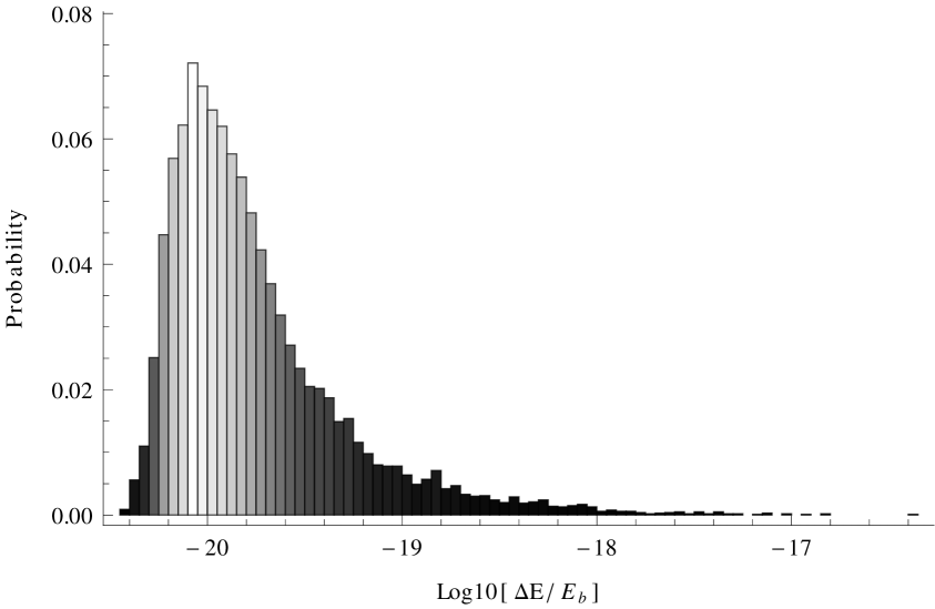
(a)

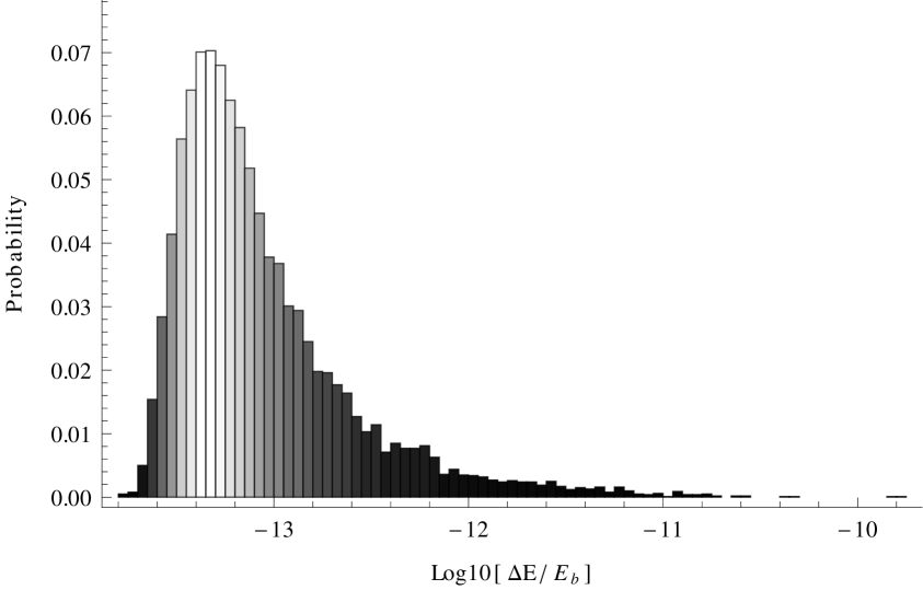
(b)

Figure 1: Resultant probability distribution of fractional energy imprinted to the Earth-Moon system due to cumulative encounters with: (a) mini-halos of mass $m_{\rm mh}=10^{-6}\textrm{M}_{\astrosun}/\textrm{AU}$, and (b) streams of linear density $\lambda_{\rm st}=10^{-6}\textrm{M}_{\astrosun}/\textrm{AU}$. The ensemble consists of about $10,000$ histories of the target evolution, under the interaction with the corresponding perturber; for about $4\,\textrm{Gyr}$ each history.

3 Application to astrophysical systems

If a population of DM mini-halos and/or streams is pervasive through the Galaxy, as some variants of DM constituents suggest, it is likely that their presence could be inferred indirectly from their cumulative dynamical effect on some astrophysical systems, which could be very sensitive to external perturbations. We now explore the consequences for two such systems.

3.1 Solar System: Earth-Moon and Neptune orbits

The Solar System dynamics is known with high accuracy. For instance, the uncertainty in the planet semi-major axis is of the order of $10^{-9}\textrm{AU}$ for Jupiter and $10^{-6}\textrm{AU}$ for Neptune [50] while for the Earth-Moon system, it is currently determined with a precision of $\Delta a/a\sim 10^{-13}$ [45]. This precision has made the Solar System to be extensively used to test general relativity, fundamental physics and alternative theories of gravity (see [51, 52, and many others] for recent examples), and it is particularly attractive to constraint the amount of DM that may be present in the Solar System [53, 54, 55, 56]. It is interesting as well to constrain the presence of dark sub-structure in the solar neighborhood.

As the Solar System moves within the Galactic halo, the orbits of planets in this system will experience almost negligible perturbations if DM is smoothly distributed, contrary to the case if it is distributed in mini-halos or streams. In the later case, the planet orbits will undergo an energy perturbation due to cumulative encounters with these structures, causing them to undergo secular evolution, and even to get unbound. We will compare the predicted dynamical effect, changes in the semi-major axis of planet orbits, principally, with the current accuracy threshold to determine upper limits on the DM sub-structure that could be present.

To start with, we choose the Sun-Neptune and Earth-Moon relative orbits as targets. Both have very stringent constraints in the determination of their semi-major axis, and they are also suitable to work within the impulsive encounter approximation. Assuming that the encounter velocity is roughly $200{\rm km/s}$, (the Sun goes around the galactic center at about $220{\rm km/s}$ and the dark halo presumably has very little rotation), means that a perturber crosses Neptune’s orbit in just $1.4\,$years, that is many times shorter than Neptune’s orbital period of $164.8\,$years; we are definitively in the impulsive regime, a similar argument applies for the Earth-Moon System. When considering cumulative encounters, we assume the encounter relative velocity magnitude to follow a Maxwell-Boltzmann distribution with a mean of $220\,{\rm km/s}$, as it is usual. Finally, we assume a standard local DM density value, $\rho_{\rm dm}=10^{-18}\textrm{M}_{\astrosun}\,\textrm{AU}^{-3}$ ($0.35\,\textrm{GeV}/\textrm{cm}^{3}$) [57, 58, 59, 60, 61] (unless otherwise is specified).

In Figure (1) we show a couple of examples of the resultant distribution for the total fractional energy, $\Delta E/E_{b}$, obtained in our Monte-Carlo experiments ensembles. Each of the runs in the ensemble corresponds to a history of encounters between the Earth-Moon system and a population of mini-halos of $m_{\rm mh}=10^{-6}\textrm{M}_{\astrosun}/{\textrm{AU}}$ (Figure ( 1(a))), or streams of $\lambda_{\rm st}=10^{-6}\textrm{M}_{\astrosun}/{\textrm{AU}}$ (Figure (1(b))). The evolution time of the system in each history is for about 4 Gyr, approximately the age of the Earth-Moon system, and the time that Neptune has been in its present orbit [62, 63]. The ensembles consists of about $10000$ histories of the target evolution. For both systems the resultant distribution is clearly non-symmetric, then we will further report the results in terms of the median value and the interquartile range.

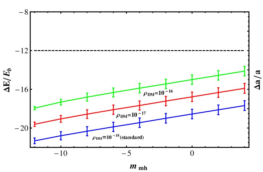
(a) Earth-Moon

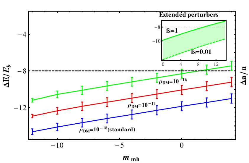
(b) Neptune

Figure 2: Constraints to the mini-halo mass due to encounters with the (a) Earth-Moon and (b) Neptune System. The median energy perturbation to the orbit, due to interactions with mini-halos as a function of their mass, compared to the experimental uncertainty in the semi-major axis of the corresponding orbit[50, 45] (dashed line). Three different values of the local DM density, $\rho_{\rm DM}(\textrm{M}_{\astrosun}/\textrm{AU}^{3})$, are shown for comparison. The bars correspond to the interquartile range for the Montecarlo realization. The sub-panel shows the effect of include the correction for extended perturbers, and that of varying the fraction of sub-structure.

First, lets take a look at the results for encounters with mini-halos. In Figures  (2(a)), and (2(b)), we summarize them, for the Earth-Moon and Neptune-sun systems, respectively. The perturber mass is in the range $10^{-12}<m_{\rm mh}<10^{4}$. We can see that none of both systems are sensitive enough to the presence of this kind of sub-structure, neither at the standard local DM density (blue line in the figures), nor at a greater values (red and green lines). Except for the most massive perturbers, more than $10^{2}\textrm{M}_{\astrosun}$, and in the denser case, $\rho_{\rm dm}>10^{-18}\textrm{M}_{\astrosun}$. This would be the maximum effect that DM mini-halos can produce, since we have assumed the fraction of mass in mini-halos equal to one and treated them as point masses. It is interesting to note that even with this extreme approximations the dynamical effect is not observable. More reliable models for mini-halos are expected to be extended and diffuse [41]. On the other hand, the fraction of substructure depends on the slope of the substructure mass function, $n$, which up to now it is only accessible by the extrapolation of it from larger scales [26]. The case of $n=-2$ would suggest that there is no smooth halo at all, and that all the mass would be contained in sub-halos. Although, current results suggest a slope of $n\sim-1.9$, implying the presence of a smooth halo component and a substructure fraction below the unity, this result may be verified by future simulations.” To consider extended mini-halos, and smaller fractions of sub-structure, would result in lower values to the injection energy, (see appendix A.1, and the sub-panel in Figure (2(b))).

Now, lets turn our attention to the interaction of these systems with dark streams; the linear mass density values used here are in the range $10^{-12}<\lambda_{\rm st}(\textrm{M}_{\astrosun}/\textrm{AU})<10^{0}$. Figures (3(a)), and  (3(b)), resumes the results. Contrary to the point mass case, both systems could be significantly affected by the presence of dark streams. At the standard value of the local DM density (blue line in the figures), the Earth-Moon system excludes the possibility of having the DM distributed on streams with $\lambda_{\rm st}\gtrsim 10^{-10}\textrm{M}_{\astrosun}/\textrm{AU}$, while the Sun-Neptune does not impose any restriction. On the other hand, if we consider higher values for the local DM density (red and green lines in figures) the constraints becomes more stringent. Both systems will be compatible with the presence of streams with linear density $\lambda_{\rm st}\lesssim 10^{-11}\textrm{M}_{\astrosun}/\textrm{AU}$, in the denser case. We initially assumed all the DM density is in streams, $\rm f_{\rm s}=1$, once we relax this condition, (shaded blue area in the plots), there are several combinations of sub-structure fraction and stream linear densities that are allowed by the observational constraints. The allowed and not allowed combinations are shown in Figure(4): a density plot for the difference between the calculated fractional change to the semi-major axis of the orbit and the observational restriction to the same quantity, the solid line indicates where the two quantities are equal, separating the region of the parameter space that is excluded (yellow-red) from that allowed (green-blue).

A more realistic situation would be one in which a fraction of the mass is in the form of streams while the rest is in mini-halos. Since the encounters with one or the other is independent. Then, in general the results will be set by the dominant specie. We can see from the plots that the dominant contribution would come from the streams in most of the cases.

(a) Earth-Moon

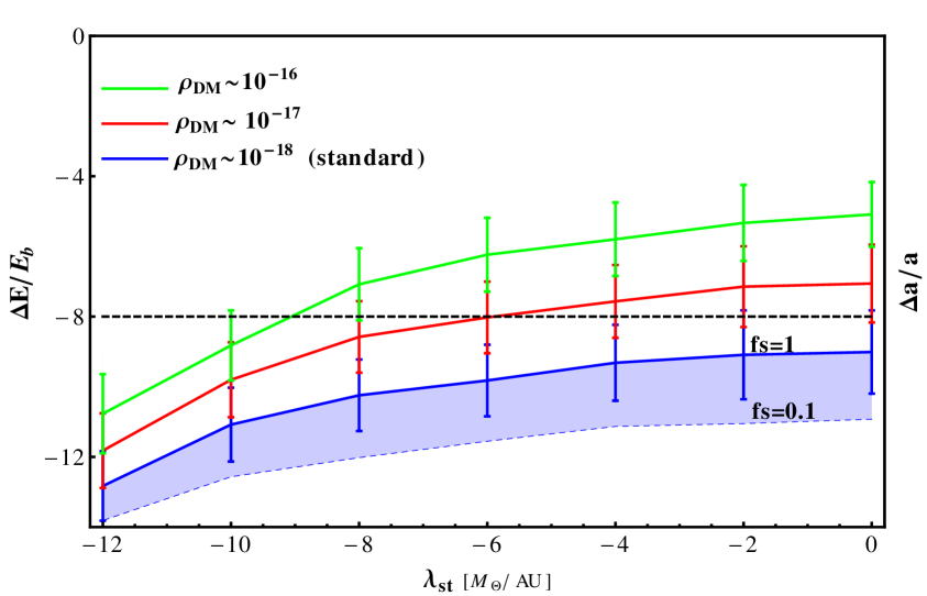
(b) Neptune

Figure 3: Constraints to linear density of dark streams due to encounters with the Earth-Moon System: We show the median energy perturbation to (a) the Earth-Moon’s orbit and (b) Neptune’s Orbit, due to interactions with dark mini-halos as a function of its mass and for three different values of the local DM density, $\rho_{\rm DM}(\textrm{M}_{\astrosun}/\textrm{AU}^{3})$. The bars correspond to the first interquartile range for the Montecarlo realization, and the dashed line to the experimental uncertainty in the semi-major axis of the orbit.

Evolution of the Astronomical Unit

There is evidence of some unexplained anomalies that concerns the astrometric data, including: the Pioneer anomaly, the variations in the astronomical unit, the Earth flyby anomaly, and the increase in the eccentricity of the Moon’s orbit (all of them discussed in [64]) . The first one has been already explained by reanalyzing the thermal radiation pressure forces inherent to the spacecraft [65], thus it has been discarded the possibility that the presence of some DMis the responsible for this anomaly. The second one remains unexplained, (see however [66]). The increase in the astronomical unit is reported to be about $15\,cm\,yr^{-1}$ [64]. We have applied our formalism of cumulative encounters with dark sub-structure to the Sun-Earth system, to check if this anomaly could be explained by the dynamic perturbations due to the presence of sub-structure. Assuming the standard local DM density value, and regardless the sub-structure fraction, neither the perturbations due to mini-halos nor due to streams, for aboutthe lifetime of the Earth, would be energetic enough to explain this anomaly. If larger values of the local density were allowed, the anomaly could be explained, however it would cause the secular evolution of other systems, like the Earth-Moon.

3.2 Wide binaries in dSphs Galaxies

It is known that binary stars systems with separations as large as $\sim 0.1\,pc$ exist in the stellar halo of the MW [67, 68], but corroborating their existence in dwarf spheroidal galaxies is an unachieved goal. The survival of these wide binaries against the interaction with the DM has been discussed before. Those in the MW had been used to set strong limits to the MACHO’s, (masive compact halos), mass[69]. And now, the existence of those in the dSph’s had been proposed as a discriminant for the DM hypotesis [47, 46]. In particular in [46] it is argued that such kind of wide binaries should be disrupted due to interaction with DM sub-halos. But, only catastrophic encounters, within the tidal interaction approach, were considered. They also assume a sub-halo mass function like the one founded in $N$-body simulations. It is important to recall that the formation process of wide binaries, and the determination of their lifetime is unclear [70, 71], as it is the assembling history of the dSph’s. This uncertainties could play an important role, when estimating the dynamical perturbations that the binaries suffer, due to the presence of dark sub-structure. According to previous studies, the existence of wide open binaries in dSphs would not be compatible with the DM hypothesis.

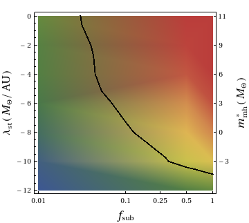
Figure 4: Fractional injection energy, for the Earth-Moon system, as a function of $\rm f_{\rm s}$ and $\lambda_{\rm st}$. The solid line is where the perturbation equals the observational limit, assuming the standard DM local density. The right axis shows a possible relation with the initial sub-halo mass, see section 4.

We study the disruption of wide binaries by means of their tidal interactions with two types of DM sub-structure: mini-halos and streams. Considering only the effect of sub-structure that is bound to the dwarf halo, and not that bounded to the MW. We can safely consider only the density of DM within the dwarf. The density of the Milky Way halo does not match that of the dSph’s at the position of the binaries, otherwise the dwarf and the binaries would be already unbounded [21]. We will follow the cumulative effect of interactions with sub-structures by means of our Monte-Carlo experiments, this will automatically take into account the diffusive and the catastrophic regime.

Such binaries could be present at a radius $r\sim 0.1\,kpc$ from the center of the dSph galaxy, where a typical value for the DM density is $\rho_{\rm dm}\sim 2.2*10^{-17}\,\textrm{M}_{\astrosun}/\textrm{AU}^{3}$, (assuming the galaxy is immersed in a NFW density profile with virial mass $M_{\rm vir}=10^{9}\textrm{M}_{\astrosun}$ and concentration $c=23.1$, as in [46]). Dwarf galaxies have typical dispersion velocities of $\sigma\approx 10{\rm km/s}$ [72]. We then assume the relative velocity of encounters to follow a Maxwell-Boltzmann velocity distribution, as in the previous section, but with a dispersion of $\sqrt{2}\sigma\sim 14\,{\rm{\rm km/s}}$. Below, we present the results obtained by following the evolution of the binaries from their interaction with dark sub-structure:

(a)

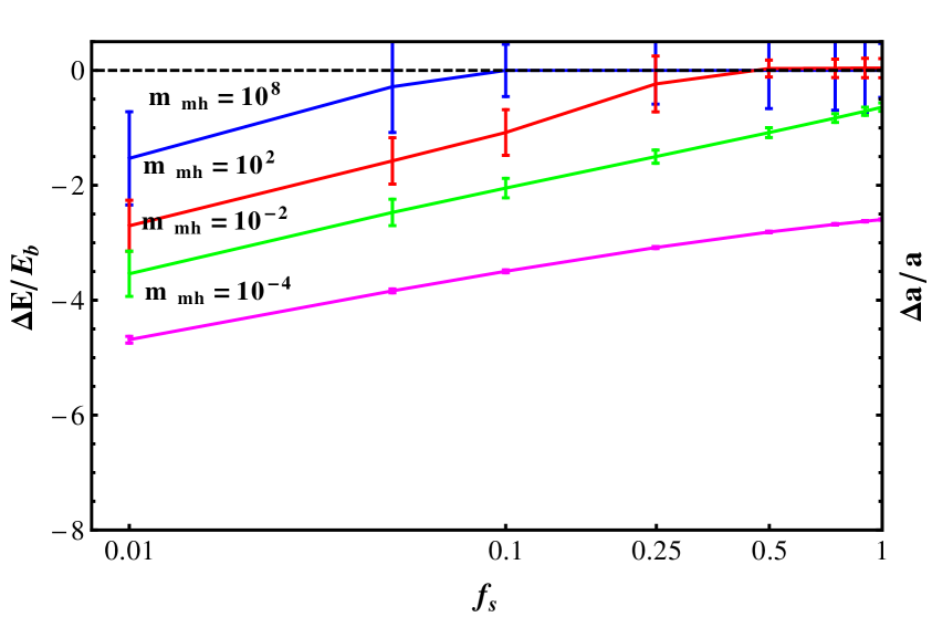
(b)

Figure 5: The median energy perturbation to a binary star system due to interaction with mini-halos. (a) As a function of the mini-halo mass, $m_{\rm mh}(\textrm{M}_{\astrosun})$ , and for three different evolution times, $t_{\rm ev}(\rm Gyr)$. (b) As a function of the fraction, $\rm f_{\rm s}$, of the mass density in mini-halos of different mass.

Interaction with mini-halos

In Figure (5(a)) we report the internal energy change, of the binary system, as a function of the perturber mass in the range $10^{-4}<m_{\rm mh}<10^{8}\textrm{M}_{\astrosun}$. For three different values of the evolution time: the solid line corresponds to the typical value assumed in previous works ($t_{\rm ev}\sim 10\,\rm{Gyr}$), and the dashed, and dotted lines correspond to shorter times ($5{\rm Gyr}$ and $2{\rm Gyr}$). The line at $\delta E/E_{b}=0$ represents the limit at which the injection energy due to encounters equals the binding energy of the binary, i.e. the moment at which the binary gets unbound. We can see that imposing a constrain to the lifetime of the binaries would impose a limit to the maximum mass of the sub-structure that could be present in the dSph’s. However, this mass limit will also depend on the fraction of the mass that is in form of mini-halos. In Figure 5(b) we show the effect of varying the sub-structure fraction for selected values of the mini-halo mass. Note that in the case of having massive perturbers, $>10^{2}\textrm{M}_{\astrosun}$ (the mass limit between the diffusive and catastrophic regime for tidal encounters set in [46]) it would be possible to unbound the binary, only if all the DM were distributed in mini-halos of this mass, and the evolution time is as large as $10\,Gyr$.The probability of having a massive perturber at short distance to the binary decrease as the impact parameter has to be larger than for the less massive perturbers. Then it would be more probable to cause the disruption of the binary by the presence of small mini-halos, than having a catastrophic encounter.

Interaction with streams

For the interaction with streams we do the same as above, but, now as a function of the linear mass density $\lambda_{\rm{st}}$. The results are shown in Figures (6(a)) and  (6(b)). Again, the binaries could be dissolved for several combinations of $\lambda_{\rm st}$, $t_{\rm ev}$ and $f_{\rm s}$. Limits to the lifetime of the binaries could impose some limits to the fraction of the mass that can be composed of dark streams of a particular linear density. For instance, if we consider that binaries have been for about $2Gyr$ under disruption, then there can not be present streams with linear densities greater that $10^{-6}\textrm{M}_{\astrosun}/\textrm{AU}$, composing more that the $10\%$ of the total DM density, otherwise the binaries would be disrupted. Similarly, if the binaries have been in the perturbation field for about $10Gyr$, then there could be present streams with $\lambda_{\rm st}<10^{-10}\textrm{M}_{\astrosun}/\textrm{AU}$, or even $\lambda_{\rm st}<10^{-8}\textrm{M}_{\astrosun}/\textrm{AU}$, depending on value of the $f_{\rm s}$ parameter. It is interesting to note that the limit to the linear mass density of streams in the later case is quite similar to that imposed by the Earth-Moon system in section 3.1.

A more general situation is that in which a fraction of the DM density mass is distributed along streams, and other in mini-halos. In this case the total energy perturbation will depend on the details of the parameters. One example is shown in Figure (7), where we compare the perturbation produced by mini-halos with that produced by the streams. The comparison is made for two values of $m_{\rm mh}$ (red) and two values of $\lambda_{\rm{st}}$ (blue). The intersection between blue and red lines shows the combination where one perturber type becomes dominant over to the other. In addition, in the case of having a smooth halo component, the fraction of mini-halos and the fraction of streams are no longer complementary, but the total perturbation effect can still be read from this plot.

3.2.1 Comparison to previous work

The disruption of Wide Binaries by their interaction with substructure was previously studied in [46]. HHere we resume the main differences, and convergence points between both approaches. In this work we do not neglect a priori the contribution of the diffusive encounters to the evolution of the binaries, but we follow the cumulative effect of encounters. In [46] all the encounters considered are in catastrophic regime. Tidal heating due to diffusive encounters produces itself a secular evolution of the binary system, and it may modify the original binary configuration before a catastrophic encounter could take place. The choice of encounter parameters in both approaches is also different. In [46] these are tied to the results of N-body simulations, instead we sample the encounter parameters from random distribution functions that depends only on the local DM density. Note that the black solid line in figure  5(a) recovers what should be expected from  [46]. Our approach allow us to study the effect of the evolution time that binaries had been perturbed, $t_{ev}$. As the evolution time decreases, the mass region for catastrophic encounters becomes smaller. Finally, we are able to study the dynamical effect due to the presence of stream-like structures, figures 6(a) and 6(b); and mixed populations of mini-halos and streams, figure 7. So far the only missing point here is to implement a relation between the perturber mass, $m_{\rm mh}$ , and the substructure fraction, $f_{s}$ , which in principle can be taken from the extrapolation of N-body simulations at larger scales [26]. Although this extrapolation may be verified in future studies, we want our approach remain as independent as possible. However, we expect that the result of including a substructure mass function in our analysis will fit in the limit cases we have already considered. Overall, we find that there is a large region in the encounter parameter space that produces secular evolution of the binary systems, then the final distribution of binary separations could not be independent of the mass and abundance of substructure, making this test not to be a sharp discriminant of the DM hypothesis as claimed in  [46]. However it would be very useful to constrain the properties of the substructure, specially when combined with other astrophysical constraints.

(a)

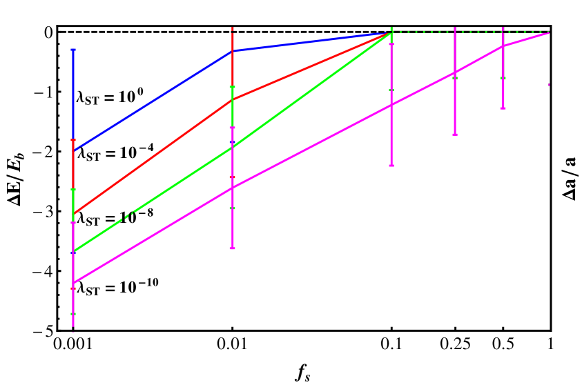
(b)

Figure 6: The median energy perturbation to a binary star system due to interaction with dark streams. (a) As a function of the stream linear mass density $\lambda_{\rm st}$ and for three different evolution times , $t_{\rm ev}(\rm Gyr)$. (b) As a function of the fraction of the mass density in streams, for four different linear mass density values.

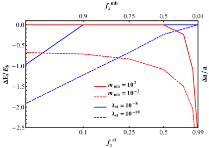
Figure 7: Binary perturbations due to the presence of mini-halos and streams. For selected values of the stream linear mass density ($\lambda_{\rm st}$, blue), an mini-halo mass ($m_{\rm mh}$, red), as a function of their corresponding sub-structure fraction. The intersection between blue and red lines shows the fraction where one perturber type becomes dominant over to the other.

4 A possible relation between $\lambda_{\rm st}$ and $m_{\rm mh}$

The actual constraints for the streams like structures could be interpreted in terms of their original mini-halo mass if we had information about the disrupted time ($t$) and how the disruption was. These two aspects are not easy to determine. We propose a very simple approach to establish this connection. Estimate the mass per unit length of a resultant stream, $\lambda_{\rm st}$, by computing first its length $L$ with the relation $L\approx\sigma_{\rm mh}\,t$ [44], which assumes that the particles moves with the velocity dispersion of the progenitor mini-halo. For simplicity, we will consider the mini-halos had an initial NFW density profile, and so the maximum velocity dispersion can be inferred from the virial mass [73] through

$$\sigma_{0}^{2} \approx 0.472V_{\rm max}^{2}$$ (4.1)

$$V_{\rm max}^{2} = \dfrac{G\,M_{\rm vir}}{2r_{s}}\dfrac{0.432}{Log[1+c]-\dfrac{c}{1+c}}$$

where $r_{s}$, and $r_{\rm vir}$ are the scale and virial radius, respectively. Use the following definitions: $r_{\rm vir}=(M_{\rm vir}/(4\pi/3\rho_{\rm cr}\Omega_{\rm m}\delta_{\rm th}))^{1/3}$ with $\rho_{\rm cr}=270.5\textrm{M}_{\astrosun}/Kpc^{3}$, the critical density of universe and $\delta_{\rm th}=340$ the predicted over-density of a collapsed object according to the top-hat collapse model for the $\Lambda-\textrm{C$\textrm{DM}$}$ model with $\Omega_{\rm m}=0.3$); and, the concentration for mini-halos $c=r_{\rm vir}/r_{s}=12*(M_{\rm vir}/h^{-1}\,10^{12})^{-0.12}$ [25]. Given the above relations, the resultant velocity dispersion for the halo mass in the range $10^{-6}<m_{\rm mh}(\textrm{M}_{\astrosun})<10^{0}$ results to be $10^{-4}<\sigma_{\rm mh}\,({\rm km/s})<10^{-2}$, so after an evolution of a Hubble time, the length of these structures would be $7<L\,(pc)<370$. Then, using a simple linear fit the relation between the mini-halo mass, and the linear mass density could be roughly set to

$$\lambda_{\rm st}\approx 10^{-8}m_{\rm mh}^{0.7}.$$ (4.2)

For instance, an initially $10^{-6}\textrm{M}_{\astrosun}$ mini-halo mass would be associated with a stream of linear density $10^{-13}\textrm{M}_{\astrosun}/\textrm{AU}$, which according to Figure (3(a)) would be perfectly allowed by the dynamics in the Solar System. For comparison we have scaled our results in Figures (4), and (6(a)), using the relation in (4.2). However, in order to have a more accurate connection between $\lambda_{\rm st}$ and $m_{\rm mh}$ an statistical study for the interaction between mini-halos and perturbers should be performed, but this is out of the scope of this work.

5 Discusion and conclusions

We have estimated the dynamical effect that sub-structure in the galactic halo may trigger on the evolution of the planet orbits in the Solar System; the Sun-Neptune and Earth-Moon orbits specifically. The effect has been compared to the current precision in the determination of their semi-major axis (known with millimeter accuracy for the Earth-Moon thanks to the APOLLO-LLR intiative [45]), finding that a local DM distribution completely populated by stream like structures with linear density of $\lambda_{\rm st}\gtrsim 10^{-10}\textrm{M}_{\astrosun}/\textrm{AU}$ in the solar neighborhood, can cause a secular evolution to the Earth-Moon system that would be above current measured limits (though Neptune orbit allows a higher value). We have also shown the allowed, and not allowed, parameter regions, in a “linear density-sub-structure fraction” space, for dark streams based on the current precision of the Earth-Moon distance measurements.

Here it is worth to emphasize the importance of the local DM density value in our study. The typical approach to constrain its value is based on dynamical studies, however, many astrophysical uncertainties are associated. According to different authors the actual limits varies from $\approx 10^{-18}\textrm{M}_{\astrosun}/\textrm{AU}^{3}$ ($(0.2-0.85)\,\textrm{GeV}\,\textrm{cm}^{-3}$) [74, 61, 60, 57, 58, 59]. Most of these studies are based on the rotation curve of the galaxy, and are subjected to the systematic errors associated to the unknown shape of the galactic halo. Other determinations of the density are local and in principle the systematic errors can be eliminated [74]. The actual data quality still needs to improve in order to get better constraints on the local DM density. The GAIA astrometric mission will improve these determinations [32, 33].

It is important, as well, to say that all these determinations only give information about the mean value, at the scale of 100’s to 1000’s of parsecs, but says nothing about the way the DM is distributed at smaller scales. Indeed, the density at the Solar System scales could show important over(under)-densities regardless of the mean value at larger scales. In this work we used different values of the local DM density, that in some cases are out of the range allowed by the current observational uncertainties. This was done in order to independently explore the space parameter. At the end, our study seems to indicate that if the Solar System DM were mainly distributed in mini-halos, the density could be an order of magnitude greater than the standard value, without being in contradiction with the Solar System dynamics and the current observational constraints described just above, but not if it is mainly distributed along streams.

We have also applied our formalism to determine if the presence of Dark Substructure in dSphs Galaxies could be in conflict with the presence of wide open binaries inside dSphs. The case of cumulative encounters, the diffusive regime, and the interaction with streams has not been considered elsewhere. We have demonstrated that catastrophic encounters are not, necessarily, the driven mechanism of destruction of wide binaries. The effect of cumulative encounters with small perturbers can cause secular evolution as well. Our results indicate that to have better constraints on the lifetime of the binaries could help to impose constraints to the properties of the dark sub-structure. But, as there are many parameter combinations, ($m_{\rm mh}$, $\lambda_{\rm st}$, $f_{\rm s}$, $t_{\rm ev}$), for which it is possible to cause secular evolution of the binary system, or even dissolve it; we consider that the existence of this kind of binaries is not a sharp discriminant of the DM hypothesis. However, to get a good characterization of their distribution would be helpful to constrain the properties of the dark sub-structure, specially when combined with other astrophysical restrictions.

Also, by relating the linear density of streams with a mini-halo progenitor mass (a simple approach) we conclude that the typical cut-off in the mas power spectrum, i.e. the mass of the smallest structures ever formed in the Universe $m_{\rm min}\sim 10^{-4}-10^{-12}\textrm{M}_{\astrosun}$ [15, 16], will correspond to streams with linear densities of $\lambda_{\rm st}\sim 10^{-11}-10^{-17}\textrm{M}_{\astrosun}/\textrm{AU}$. Such values are compatible with the dynamics of the solar system (a similar conclusion was obtained when we consider the mini-halos as a point mass perturbers), and would be compatible also with the existence of wide binaries in dSph’s, if they were to be detected. On the other hand, for streams with $\lambda\approx 10^{-10}$–$10^{-8}\textrm{M}_{\astrosun}/\textrm{AU}$ ($m_{\rm min}\sim 10^{-3}-10^{0}\textrm{M}_{\astrosun}$), the fractional energy imprinted to the binary stars would cause their disruption, and the corresponding effect to Earth-Moon system would be just below (or above) the observational restriction. That is, if wide binaries in dSph’s with separations of $a\sim 0.1pc$ were not observed, it could be due to the presence of streams with $\lambda_{\rm st}>10^{-10}\textrm{M}_{\astrosun}/\textrm{AU}$ ($m_{\rm min}\sim 10^{-3}$), but the presence of such kind of structures in the solar neighborhood would (likely) be incompatible with the Earth-Moon dynamics (although it depends in the sub-structure fraction). This is an example of how the combined restrictions, from different astrophysical systems, could be revealing the sub-structure mass function cut-off scale.

Finally, we want to make some comments regarding the direct, and indirect DM detection methods. First, it is well known that the presence of dark mini-halos, or streams, in the solar neighborhood, could affect the event rate and energy spectrum, and consequently the exclusion limits set by current experiments. From our study, we can say that the dynamics of the Solar System is not significantly affected by the presence of both kind of sub-structures, mini-halos and streams (not even in the idealized case when the sub-structure fraction is equal to one). This rise up the possibility of being in a over-dense region and suggest that DM halo models that includes the presence of DM sub-structure should be used when interpreting experimental results. However, there is also the possibility to be in a under-dense region, not distinguishable from the standard case by dynamical studies, but with important consequences for the direct detection methods.

On the other hand, the presence of dark sub-structure in galactic halos, could also affect the interpretation of the results for DM indirect detection experiments, because in some cases it is subjected to the use of a boost factor mechanism, usually associated to the Sommerfeld enhancement, that is velocity dependent. As mini-halos and streams are, in general, kinematically colder than a soft galactic halo, then, the limits to the sub-structure properties set in this work could be useful also to interpret the results of DM indirect detection experiments .

Appendix A Corrections for Spherical models.

A.1 Correction for extended perturbers.

In this section we present the behavior of the $U$ function, in equation (2.1), that accounts for the extension and structure of the dark mini-halos. For this we have assumed the mini-halos have a NFW mass profile, normalized to the virial mass, of the form:

$$\mu(r/r_{s})=\dfrac{1}{\log(1+c)-\dfrac{c}{1+c}}\,\left(\log\left[1+r/r_{s}\right]-\dfrac{r/r_{s}}{1+r/r_{s}}\right),$$ (A.1)

where $c=r_{\rm vir}/r_{s}$ is the concentration; $r_{s}$ and $r_{\rm vir}$ are the scale and virial radius respectively. Following [49], and given that the mass profile is normalized to the virial mass, we will define the $U$ function as:

$$U(\xi)= \int_{1}^{\infty}{\mu(p\,\xi)\,\xi^{-2}(\xi^{2}-1)^{-1/2}}d\xi\quad\mbox{for}\quad p/r_{s}<c$$

$$U(\xi)= \int_{1}^{\infty}{\xi^{-2}(\xi^{2}-1)^{-1/2}}d\xi=1\quad\mbox{for}\quad p/r_{s}>c$$ (A.2a)

After integration, the $U$ function takes the form

$$U(\xi)= \dfrac{\dfrac{{\rm ArcSec}[p]}{\sqrt{-1+p^{2}}}+\log\left[\frac{p}{2}\right]}{\left(-\frac{c}{1+c}+\log[1+c]\right)}\quad\mbox{for}\quad p/r_{s}<c$$

$$U(\xi)= 1\quad\mbox{for}\quad p/r_{s}>c,$$ (A.3a)

and it is ploted in Figure, 8, for different values of the mini-halo mass. The $U$ function crosses the point mass approximation at $r/p=c$ for the different masses. For comparison we added a line for the point mass case ($U_{\rm NFW}=1$), to see the scale at which this becomes valid. We have seen this correction is less important for small mini-halos.

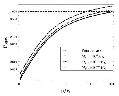
Figure 8: Structure function, $U$, for halos with a NFW density profile, as a function of their mass. For comparison we added a line for the point mass case ($U_{\rm NFW}=1$), to see the scale at which this becomes valid.

A.2 Corrections for non-distant tide encounters.

In this section we deal with encounters where the distant tide approach is not applicable. In particular, this happens when we study the interaction of wide binaries with point mass (or spherical) dark sub-structure present in the MW satellites. We will use the this system to state the problem, and the solution, but this can be applied to other systems for which the distant approximation does not applies.

The distant tide approximation is valid when the size of the target system is much smaller than the impact parameter. Te determine whether this condition is satisfied, or not, we consider the characteristic of the wide binaries and DM sub-structure we used in Sec.3.2 ($\rho_{\rm dm}=2.210^{-17}\textrm{M}_{\astrosun}/\textrm{AU}^{3}$, a=$0.1pc$, $M_{b}=1\textrm{M}_{\astrosun}$, etc.). We can compare the binary separation with the mean impact parameter for the encounters, $<p>=\Gamma(1/3)\,(36\,\pi\,\rho_{\rm dm}/m_{\rm mh})^{(-1/3)}$ (defined from the nearest neighbor distribution), for different values of the perturber mass. Table 9(a) shows this comparison: values lower or close to one implies that distant tide approximation is not applicable. For the less massive perturbers, most of the encounters could not be treated in the distant tide approximation. Since the sampling of impact parameters is random, we do not know, a priori, which of the encounters could be treated in the distant approximation and which not. In the practice we have to make this comparison for each encounter, then we decide if it is appropriate to use the distant tide approximation, or to directly calculate the velocity kick to each component of the binary, and calculate the input energy as we describe in the following paragraphs.

$m_{\rm mh}(\textrm{M}_{\astrosun})$	$p/a$
$10^{-6}$	0.33
$10^{-4}$	1.55
$10^{-2}$	7
$1$	33
$10^{2}$	155
$10^{6}$	335

(a)

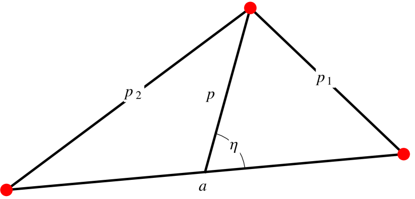
(b)

Figure 9: (a) Shows the factor $p_{\rm mean}/a$ for different values of the mass perturber. Values close to one means that the distant approximation, in the calculation of the dynamical effect of encounters between a target and a population of mimi-halos, is not applicable. (b) Diagram that shows the definitions used to calculate the correction for non-distant encounters with mini-halos.

For each component of the binary the kick in velocity due to an encounter, in the non-distant tide approach, is given by

$$\Delta\mathbf{v}_{i}=\dfrac{2GM_{p}}{v}U(p_{i})\dfrac{\hat{\mathbf{p}_{i}}}{p_{i}}$$ (A.4)

where $U(p)$ is a function that depends on the perturber density profile, and tends to one when the impact parameter ($p$) is larger compared with the size of the perturber (this correction is described in detail in [49], and in appendix A.1). The subscript $i$ refers to the $i$-th component of the binary. The differential energy per unit mass transferred to the binary system is

$$\Delta E=0.5\Delta v_{\rm diff}^{2}+\mathbf{v}\cdot\Delta\mathbf{v}$$ (A.5)

where $\Delta v_{\rm diff}=\left|\Delta\mathbf{v}_{2}-\Delta\mathbf{v}_{1}\right|$, is the vector difference of the individual contributions of both components of the binary system.

In our approach the magnitude of the impact parameter is sampled from a nearest neighbor distribution, so we have to assume respect to what point point of the binary it is referred, by simplicity we will assume it is respect to the center of mass, so that the individual impact parameters to the binary components are given by:

$$p_{1}^{2}=p^{2}+(a/2)^{2}-p\,a\,\cos{\eta}$$

$$p_{2}^{2}=p^{2}+(a/2)^{2}+p\,a\,\cos{\eta}$$ (A.6)

where $\eta$ is the relative direction between the imaginary line that connects the binary, and the one that draws the impact parameter direction (we will sample this angle from a uniform distribution between $0$ and $\pi$, since it is equally probably to have any orientation of the binary). Given this geometry we rewrite eq. (A.5) in terms of the impact parameters and the binary separation.

$$\Delta E = 0.5\left(\dfrac{2GM_{p}}{v}\right)^{2}\delta v_{\rm tot}^{2}\;\;\;\;\;\mbox{where}$$

$$\delta v_{\rm tot}^{2} = \delta v_{1}^{2}+\delta v_{2}^{2}-2\delta\mathbf{v}_{1}\cdot\delta\mathbf{v}_{2}$$ (A.7)

$$= \left(\dfrac{U(p_{1})}{p_{1}}\right)^{2}+\left(\dfrac{U(p_{2})}{p_{2}}\right)^{2}-2\dfrac{U(p_{1})\,U(p_{2})(p_{1}^{2}+p_{2}^{2}-a^{2})}{p_{1}^{2}\,p_{2}^{2}}$$

This last expression is used whenever the condition of distant tide encounters, in our analysis, is not satisfied. Note we have neglected the linear velocity term in eq (A.5), beacuse we expect it approaches to zero when $\Delta E$ is summed over all the encounters as a result of symmetry (See [49]).

Appendix B Stream models

B.1 Derivation of tidal perturbation.

In this appendix we derive analytical expressions for the force and tidal fields produced by the stream models we have considered. All of them present axial symmetry. Our simplest model is a 1-dimensional mass distribution with linear mass density $\lambda_{\rm st}$ (S-1D). Then we consider a stream with finite cross section of radius $R_{o}$ and constant cross–sectional density $\Sigma_{o}$ (S-CD). Finally, we consider streams whose cross-sectional densities vary as power laws with central cores (S-Core), or cusps (S-Cusp):

$$\Sigma\left(R;R_{o},\alpha,\gamma\right)=\Sigma_{o}\,\left(R/R_{o}\right)^{-\alpha}\,[1+\left(R/R_{o}\right)]^{\alpha-\gamma},$$ (B.1)

where $\Sigma_{o}$ is a scaling density parameter, $R_{o}$ a characteristic radius and $\alpha$, $\gamma$ are dimensionless exponents that satisfy:

$$0\leq\alpha<2,\,\,\gamma>2.$$ (B.2)

The restriction $\alpha\geq 0$ is to avoid an inverted density profile at the center, while $\alpha<2$ avoids an infinite mass singularity there ($0<\alpha<2$ produces a finite mass singularity). The restriction $\gamma>2$ is to have a finite mass per unit length. When $\alpha=0$ we have the flat core cases, whereas for $\alpha>0$ we have the cusp cases.

Force field

The force field can be obtained using the integral Poisson equation:

$$\int\nabla\cdot{\bf F}\,dV=-4\,\pi\,G\,M.$$ (B.3)

Taking advantage of the axial symmetry of the problem, the resulting forces are given by:

$$F^{S-1D}\left(R\right)= -\dfrac{2G\lambda_{\rm st}}{R},$$ (B.4)

$$F^{S-CD}\left(R\right)= -F_{o}\,\dfrac{{\left(Min[\eta,1]\right)}^{2}}{\eta},$$ (B.5)

$$F^{S-Core}\left(R\right)= -F_{o}\,\dfrac{\eta^{2}-\gamma\eta\left(1+\eta\right)+{\left(1+\eta\right)}^{\gamma}-1}{\eta{\left(1+\eta\right)}^{\gamma}},$$ (B.6)

$$F^{S-Cusp}\left(R\right)= -F_{o}\,\dfrac{1-{\left(1+\eta\right)}^{2-\gamma}}{\eta}\,\,\,\,\,\,\left(\alpha=1\right),$$ (B.7)

where we have introduced the dimensionless length $\eta=R/R_{o}$ and $F_{o}\equiv 2G\lambda_{\rm st}/R_{o}$, with $\lambda_{\rm st}$ equal to the total mass per unit length (integrated across the stream cross section). All forces are orthogonal to the stream and directed towards it. For the cusp case there is no general analytical expression, so we show the special $\alpha=1$ case, which is the only cusp model we will consider from now on.

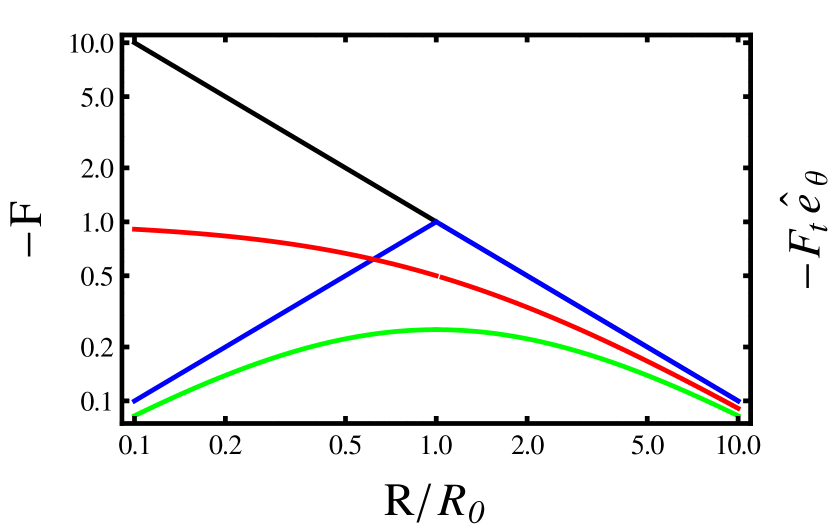
(a) Magnitude of the force produced by our stream models as a function of distance to the stream central axis, $R$. It coincides with the tidal force in the $\theta$ direction, equation (B.10).

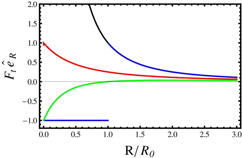
(b) Magnitude of the tidal force, in the $R$ direction, produced by our stream models as a function of distance to the stream central axis, $R$.

Figure 10: The curves are for the 1-D (black), constant density (blue), core (green) and cusp (red) models. In each case, we set $\lambda_{\rm st}$, $F_{0}$ and $\zeta_{0}$ to the unity. For the core and cusp models $\gamma=3$ is assumed.

Figure (10(a)) shows these forces, for streams with $\lambda_{\rm st}=1$, or $F_{0}=1$, accordingly; and $\gamma=3$ for the core and cusp models is assumed. We see that the S-1D and S-CD models coincide for $R>R_{o}$, but whereas the former diverges toward the center, the latter converges linearly to zero. The core model goes also to zero at the center, while the cusp model does not and so the force is discontinuous at the stream axis. For large $R$ all models coincide, as they should, since they become indistinguishable.

Tidal force field

The components of the tidal force produced by a force field ${\bf F}$ on a target of size $d{\bf r}$ at position ${\bf r}$, in the linear approximation, (we use general coordinates $x^{\alpha}$ and Einstein’s sumation convention), is given by :

$${F_{t\,x_{\alpha}}}=-\dfrac{\partial{F}_{\alpha}}{\partial x_{\beta}}dx^{\beta}=\tau_{\alpha\,\beta}dx^{\beta}$$ (B.8)

The tensor $\tau$, a symmetric and second rank tensor, is the Jacobian of the gravitational force field ${\bf F}$, and the negative of the Hessian matrix, $H$, of the scalar potential function $\Phi$. The tensor $\tau$ can be written in any curvilinear coordinates by means of the covariant derivative, [See appendix A of reference 77, for a detailed explanation], i.e.

$$\tau_{\alpha,\beta}=-H_{\alpha\,\beta}\left(\Phi\right)=F_{\alpha,\beta}-\Gamma^{\gamma}_{\alpha\,\beta}F_{\alpha},$$ (B.9)

where, ${\bf F}=-{\bf\nabla}\Phi$. The Christophel symbols, $\Gamma$, and the force ${\bf F}$, must be written in the selected coordinate system. For our specific case of streams with axial symmetry, it is convenient to use cylindrical coordinates, defined as in Figure (11(a)); then, in this particular case the tidal force takes the form:

$${\bf F}_{t}\left({\bf r},d{\bf r}\right) = \tau_{r\,r}\,dr\,\hat{\bf e}_{r}+\tau_{\theta\,\theta}\,r\,d\theta\,\hat{\bf e}_{\theta}$$ (B.10)

$$= \dfrac{\partial F\left(r\right)}{\partial r}dr\,\hat{\bf e}_{r}+F\left(r\right)d\theta\,\hat{\bf e}_{\theta}.$$

Using the expressions for the force of each of our stream models, eqs. (B.4) to (B.7) respectively, it is straightforward to obtain the expressions for the corresponding tidal forces, given by eq. (B.10). As an example, the tidal force in the 1-D stream case is,

$$\mathbf{F}_{t}^{S-1D}=\dfrac{2\,G\,\lambda_{\rm st}}{R^{2}}dr\,\hat{\mathbf{e}}_{r}-\dfrac{2\,G\,\lambda_{\rm st}}{R}d\theta\,\hat{\mathbf{e}}_{\theta},$$ (B.11)

Figure (10(b)) shows radial component of the tidal forces, for streams with $\lambda_{\rm st}=1$, or $F_{0}=1$, accordingly; and $\gamma=3$ for the core and cusp models is assumed. For the S-1D and S-CD models is the same stretching force outside the stream; once inside the finite thickness stream, the tidal effect turns into a constant compression. The Core stream presents a simmilar behaivor as the S-CD, i.e, in some range gives a compresive force, and in other a streaching one. The Cusp stream gives always a compresive force. The tangential component of the tidal force coincides with the force, and the effect is always compressive for all the models.

The fractional energy change

Now, to quantify the effect of an encounter with a stream we will focus on changes to the internal energy of the target, which is mostly kinetic. One needs to compute the integral of the tidal force over time to get the kick in the velocity during to the encounter with a stream,

$$\delta\mathbf{v}=\int{\mathbf{F}_{t}\left(\mathbf{R},\delta\mathbf{r}\right)}\;\rm{d}t,$$ (B.12)

where $\mathbf{R}$ is the cylindrical position vector of the target center with respect to the closest stream point, and $\delta\mathbf{r}$, is the position vector of an element of the target, with respect to the target center. Both, $\mathbf{R}$ and $\delta\mathbf{r}$ are functions of time. The integral in eq.(B.12) should be made over the time that the encounter takes place, in general this could be accomplished by means of numerical simulations. However, this problem can be treated analytically in two opposite regimes: If the encounter time is a lot shorter than the internal dynamical time of the target, then we can take $\delta\mathbf{r}$ as fixed and just take into account the variation of $\mathbf{R}(t)$, this is the so called, impulsive regime. The opposite regime is when the encounter time is a lot longer than the internal dynamical time of the target. In this case we can average the effect of the tidal force over an entire dynamical timescale of the target and then use the average force as the integrand in eq. (B.12), this is the adiabatic regime.

The systems of interest to this work are suitable to be worked in the impulsive regime, so we will estimate the effect of a single encounter using this approximation. The kick in velocity will be obtained by eq. (B.12) once we substitute the corresponding tidal force, (B.10), for the different models. But before doing this we must consider the geometry of the problem. There are two issues here: first, the geometry of the encounter stream-target will define the form of $\mathbf{R}(t)$; and second, the orientation of the target with respect to the stream will define the components of $\delta\mathbf{r}$.

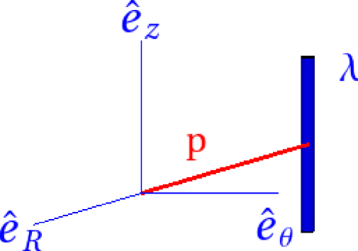
(a)

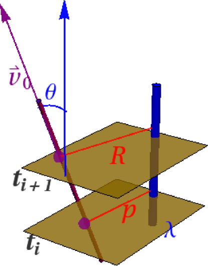
(b)

Figure 11: (a)Coordinate frame used for the tidal tensor computation. (b) Relative direction of movement definition.

The geometry of the encounter stream-target

Let us introduce here the concept of the impact parameter, $p$, for encounters with streams. It will be defined as the closest distance between the stream and the target, with the particularity that it will always be orthogonal to the to the $z$ axis of the cylinder. Now, lets see the relation of the impact parameter with the vector position $R$ of the target with respect to the stream. Lets suppose we define the impact parameter at the time $t=t_{i}$, it should lie in the plane normal to $z$. At this time the impact parameter, $p$, and the vector position $R$ coincide. Now as the time evolve, the target will move, in some direction with respect to the stream, so that the vector position will not coincide any more with the impact parameter. The difference between them will be just the distance the target, moving at velocity $v_{0}$ relative to the stream, has traveled. This distance will depend the relative direction of movement between the stream and target, being $\theta$ the angle that characterize this relative direction, as it is shown in Figure (11(b)). So, the equation that gives the temporal variation of the target-stream magnitude vector position, $R$, is:

$$R\left(t;p,\theta,v_{0}\right)=\sqrt{p^{2}+\left(v_{0}\,t\sin\theta\right)^{2}}$$ (B.13)

One can verify that $\theta=0$ correspond to the case in which the stream and target are moving parallel, at constant impact parameter.

The geometry of the target orientation

Now it is time to turn our attention to the orientation of the target with respect to the stream. What we need to do is to express the vector position of an element of the target, $\delta{\bf r}$, in the reference frame defined by the stream (Figure 11(a)), that is to express $\delta\mathbf{r}$ with respect to the triad of unit vectors $(\hat{e}_{R},\hat{e}_{\theta},\hat{e}_{z})$.

One can describe this transformation by means of a three angle rotation:

1. Rotation of the target plane by an angle $\alpha$ with respect to the $\hat{e}_{\theta}$ axis (Figure 12(a)).

2. Rotation of the target plane by an angle $\beta$ with respect to the original $\hat{e}_{z}$ axis (Figure 12(b)).

3. Rotation on the target plane by an angle $\psi$ with respect to the normal $\hat{e}_{n}$ of the target plane (Figure 12(c)).

The first 2 angles defines the spatial orientation of the target plane with respect to the stream plane, the third angle is just the orbital phase of the target, see Figure 12 for clarification in the definition of the angles. It is clear that $-\pi/2\leq\alpha\leq\pi/2$, $0\leq\beta\leq\pi$, and $0\leq\psi\leq 2\,\pi$. The rotation matrix for the individual rotations are:

$$\begin{array}[4cm]{ccc}\lambda_{\beta}=\left(\begin{array}[]{ccc}\cos\left(\beta\right)&\sin\left(\beta\right)&0\\ -\sin\left(\beta\right)&\cos\left(\beta\right)&0\\ 0&0&1\end{array}\right),&\lambda_{\alpha}=\left(\begin{array}[]{ccc}\cos\left(\alpha\right)&0&-\sin\left(\alpha\right)\\ 0&1&0\\ \sin\left(\alpha\right)&0&\cos\left(\alpha\right)\end{array}\right),&\lambda_{\psi}=\left(\begin{array}[]{ccc}\cos\left(\psi\right)&\sin\left(\psi\right)&0\\ -\sin\left(\psi\right)&\cos\left(\psi\right)&0\\ 0&0&1\end{array}\right).\end{array}$$ (B.24)

To get the proper final rotation, we should apply them in the order: first the $\beta$-rotation, followed by the $\alpha$-rotation and finally the $\psi$-rotation. The inversion in the order of the first two is so that the pivot for the $\alpha$-rotation is with respect to the rotated $\hat{e}_{\theta}$ axis. If we do it in the inverse order, then the pivot for the second rotation ($\beta$) is the original $\hat{e}_{z}$ axis, and not its transformed version, which complicates the algebra. The expression of vector $\delta\mathbf{r}$ using in reference frame attached to stream, then, is:

$$\delta\mathbf{r} = \delta r\left\{\left[\cos\left(\alpha\right)\,\cos\left(\beta\right)\cos\left(\psi\right)-\sin\left(\beta\right)\,\sin\left(\psi\right)\right]\hat{\mathbf{e}}_{R}\right.$$ (B.25)

$$+ \left.\left[\cos\left(\alpha\right)\,\cos\left(\beta\right)\sin\left(\psi\right)+\cos\left(\beta\right)\,\sin\left(\psi\right)\right]\,\hat{\mathbf{e}}_{\theta}-\left[\cos\left(\psi\right)\sin\left(\alpha\right)\right]\hat{\mathbf{e}}_{z}\right\}$$

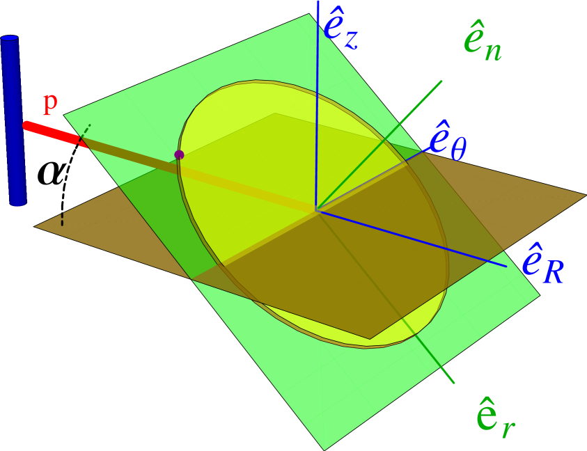
(a)

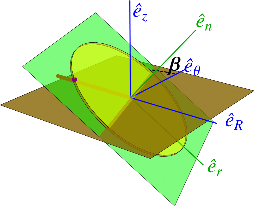
(b)

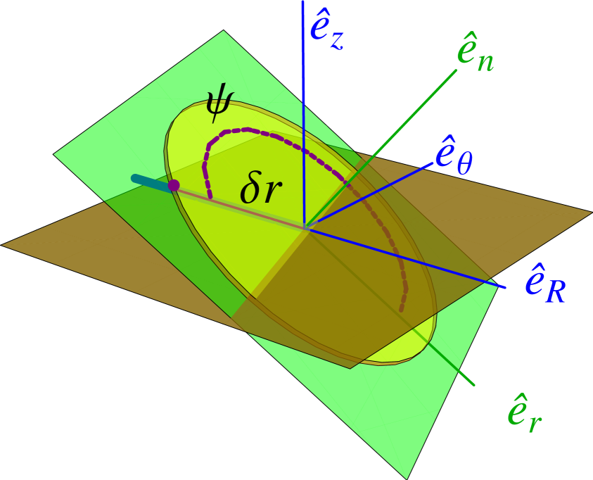
(c)

Figure 12: We show the definitions of the rotation angles $\alpha$, $\beta$ and $\psi$ that allow us to write the vector position of an element of the target, $\delta r$ (that lies in the target plane –green–), in the stream reference frame coordinates (brown plane).

Finally, the perturbation energy (per unit mass) transfered to the internal dynamics of an extended target system, by one single stream encounter, is simply

$$\Delta E=\Delta(1/2v^{2})=(\mathbf{v}\cdot\Delta\mathbf{v})+1/2(\Delta\mathbf{v})^{2}\sim 1/2(\Delta v)^{2}$$ (B.26)

where in the last step, we have neglected the linear term between the velocity of the target planet, $\mathbf{v}$, and the tidal velocity kick, $\Delta\mathbf{v}$ (random orientation). We now compare this perturbation energy with the binding energy of the target: $E_{b}=-G\,M_{\rm c}/(2\,a)$, and substitute equations (B.25) and (B.10) in eq.(B.12). The integration was done considering $\delta{\bf r}$ constant, i.e. $\delta r,\alpha,\beta$ and $\psi$ constants during the encounter. The results are the following, for the different stream models.

$$\dfrac{\langle\Delta E\rangle_{\rm st}}{|E_{b}|}=\dfrac{4\,G\,\pi^{2}\lambda^{2}}{M_{c}\,v^{2}_{0}\,{\sin\left(\theta\right)}^{2}\,p^{2}}a^{3} \varmathbb{T}\left(\alpha,\psi\right)$$ (1D) (B.27a)

$$\dfrac{\langle\Delta E\rangle_{\rm st}}{|E_{b}|}=\dfrac{4\,G\,\pi^{2}\lambda^{2}}{M_{c}\,v^{2}_{0}\,{\sin\left(\theta\right)}^{2}\,p^{2}}a^{3} \varmathbb{T}\left(\alpha,\psi\right)\,{\varmathbb{B}^{2}\left(R_{0}/p\right)}$$ (CD) (B.27b)

$$\dfrac{\langle\Delta E\rangle_{\rm st}}{|E_{b}|}=\dfrac{4\,G\,\pi^{2}\lambda^{2}}{M_{c}\,v^{2}_{0}\,{\sin\left(\theta\right)}^{2}\,p^{2}}a^{3} \varmathbb{C}\left(R_{0}/p,\alpha,\beta,\psi\right)$$ (Core) (B.27c)

$$\dfrac{\langle\Delta E\rangle_{\rm st}}{|E_{b}|}=\dfrac{4\,G\,\pi^{2}\lambda^{2}}{M_{c}\,v^{2}_{0}\,{\sin\left(\theta\right)}^{2}\,p^{2}}a^{3} \varmathbb{D}\left(R_{0}/p,\alpha,\beta,\psi\right)$$ (Cusp). (B.27d)

where the geometric functions, $\varmathbb{T}$, $\varmathbb{B}$, $\varmathbb{C}$, and $\varmathbb{D}$ are given by:

$$\varmathbb{T} = \left[\cos^{2}\left(\alpha\right)\,\cos^{2}\left(\psi\right)+\sin^{2}\left(\psi\right)\right]$$ (B.28)

$$\varmathbb{B} = \frac{2}{\pi}\left[\arctan\left(\frac{R_{0}/p}{\sqrt{1-R_{0}/p^{2}}}\right)-R_{0}/p\sqrt{1-R_{0}/p^{2}}\right]\qquad R_{0}/p\leq 1$$

$$= 1,\qquad\qquad\qquad\qquad\quad\qquad\qquad\qquad R_{0}/p\geq 1$$

$$\varmathbb{C} = {I_{1}}^{2}(R_{0}/p)\left[\cos\left(\alpha\right)\,\cos\left(\beta\right)\,\cos\left(\psi\right)-\sin\left(\beta\right)\,\sin\left(\psi\right)\right]^{2}+$$

$${I_{2}}^{2}(R_{0}/p)\left[\cos\left(\alpha\right)\,\cos\left(\psi\right)\,\sin\left(\beta\right)+\cos\left(\beta\right)\sin\left(\psi\right)\right]^{2},$$

$$\enskip I_{1}=\frac{2}{\pi}\int_{0}^{\infty}{\frac{\sqrt{1-\tau^{2}}-R_{0}/p}{\left[\sqrt{1+\tau^{2}}+R_{0}/p\right]^{3}}d\tau}$$

$$\enskip I_{2}=\frac{2}{\pi}\int_{0}^{\infty}{\frac{1}{\left[\sqrt{1+\tau^{2}}+R_{0}/p\right]^{2}}d\tau}$$

$$\varmathbb{D} = {I_{3}}^{2}(R_{0}/p)\left[\cos\left(\alpha\right)\,\cos\left(\beta\right)\,\cos\left(\psi\right)-\sin\left(\beta\right)\,\sin\left(\psi\right)\right]^{2}+$$

$${I_{4}}^{2}(R_{0}/p)\left[\cos\left(\alpha\right)\,\cos\left(\psi\right)\,\sin\left(\beta\right)+\cos\left(\beta\right)\sin\left(\psi\right)\right]^{2},$$

$$\enskip I_{3}=\frac{2}{\pi}\int_{0}^{\infty}{\frac{d\tau}{\left[R_{0}/p\,\sqrt{1+\tau^{2}}\right]^{2}}d\tau}$$

$$\enskip I_{4}=\frac{2}{\pi}\int_{0}^{\infty}{\frac{d\tau}{\sqrt{1+\tau^{2}}\left[R_{0}/p+\sqrt{1+\tau^{2}}\right]}d\tau}$$

All the functions $\Delta E/E_{b}$ for the different models, converge to that of the S-1D model for large impact parameters, see Figure 13(a).

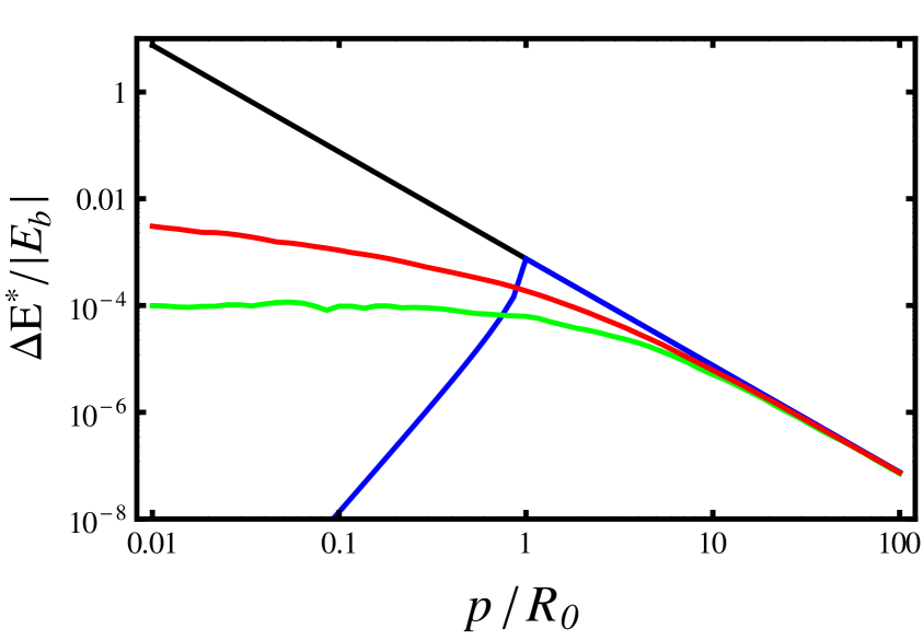
(a) Perturbation energy produced by the streams, as a function of the impact parameter, $p$. The models are the same as in Figure 10(a)

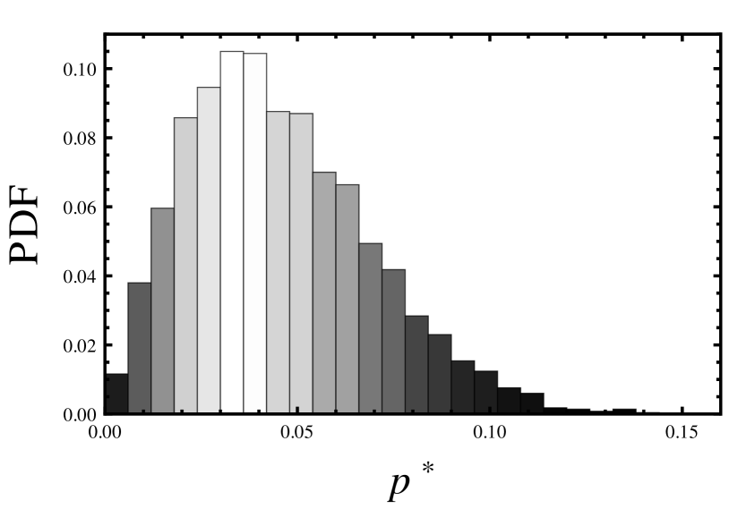
(b) Impact parameter probability distribution functions for dark streams calculated by the sampling procedure described in the text.

Figure 13:

B.2 Impact parameters for streams.

In order to generate the distribution function of impact parameters for the streams, we follow the next procedure. We start by tossing a given number of random lines within a region of the 3D-space. Then we also tose a collection of uniformly distributed points, within the same region, and determine the distance from each point to the closest line, that is the impact parameter. This results in a sampling of the underlying distribution of impact parameters that is completely independent of the introduction of a sample volume. We show the resultant probability distribution in Figure (13(b)). We still need to relate this realization to a specific distribution of matter with a certain spatial mass density, $\rho$, and linear mass density for the lines, $\lambda$, so that the impact parameter denoted by $p^{*}$ can have the correct dimensions according to the specific physical situation. The way to do this to introduce a sample volume to measure the mass density around each of the tests points. We did several experiments, keeping fixed the total number of lines in the realization, as well as the realization volume, but changing the size of the sample volume, $R^{*}$, and we found that the number density of streams varies with it, but the mass density doe not. Thus, in our procedure, the mass density is a well defined physical quantity whose value is independent of the size of the region used to compute it. In the practice, we normalized the linear mass density of the streams to the unity so that the mass density we get from the realization is $\rho^{*}$. By doing a dimensional analysis we get to the conclusion that the relation between the impact parameter, $p^{*}$, and the physical impact parameter $p$, is given by: $p=\left(\sqrt{\lambda_{\rm st}\,\rho^{*}/\rm f_{\rm s}\,\rho}\right)\,p^{*}$, where $\lambda_{\rm st}$ and $\rho$ are given in physical units, and $\rho^{*}$ is the numerical mass density obtained in a given realization.
We will use the impact parameter distribution function shown in Figure 13(b), that corresponds to a numerical mass density of $\rho^{*}=1205.08$; the $\lambda_{\rm st}$, $\rm f_{\rm s}$, and $\rho$ parameters will be fixed according to the specific situation under study.

References

- [1] WMAP Collaboration Collaboration, E. Komatsu et. al., Five-Year Wilkinson Microwave Anisotropy Probe (WMAP) Observations: Cosmological Interpretation, Astrophys.J.Suppl. 180 (2009) 330–376, [arXiv:0803.0547].
- [2] SDSS Collaboration Collaboration, M. Tegmark et. al., Cosmological Constraints from the SDSS Luminous Red Galaxies, Phys.Rev. D74 (2006) 123507, [astro-ph/0608632].
- [3] S. Dye and S. Warren, Constraints on dark and visible mass in galaxies from strong gravitational lensing, IAU Symp. (2007) [arXiv:0708.0787].
- [4] M. Viel, G. D. Becker, J. S. Bolton, M. G. Haehnelt, M. Rauch, et. al., How cold is cold dark matter? Small scales constraints from the flux power spectrum of the high-redshift Lyman-alpha forest, Phys.Rev.Lett. 100 (2008) 041304, [arXiv:0709.0131].
- [5] D. Clowe, M. Bradac, A. H. Gonzalez, M. Markevitch, S. W. Randall, et. al., A direct empirical proof of the existence of dark matter, Astrophys.J. 648 (2006) L109–L113, [astro-ph/0608407].
- [6] G. Steigman and M. S. Turner, Cosmological constraints on the properties of weakly interacting massive particles, Nuclear Physics B 253 (1985) 375–386.
- [7] G. Jungman, M. Kamionkowski, and K. Griest, Supersymmetric dark matter, Phys.Rept. 267 (1996) 195–373, [hep-ph/9506380].
- [8] N. Menci, F. Fiore, and A. Lamastra, Galaxy Formation in WDM Cosmology, MNRAS 421 (2012) [arXiv:1201.1617].
- [9] V. Avila-Reese, P. Colin, O. Valenzuela, E. D’Onghia, and C. Firmani, Formation and structure of halos in a warm dark matter cosmology, Astrophys.J. 559 (2001) 516–530, [astro-ph/0010525].
- [10] U. Seljak, A. Makarov, P. McDonald, and H. Trac, Can sterile neutrinos be the dark matter?, Phys.Rev.Lett. 97 (2006) 191303, [astro-ph/0602430].
- [11] A. X. Gonzalez-Morales, R. Poltis, B. D. Sherwin, and L. Verde, Are priors responsible for cosmology favoring additional neutrino species?, arXiv:1106.5052.
- [12] M. Archidiacono, E. Calabrese, and A. Melchiorri, The Case for Dark Radiation, Phys.Rev. D84 (2011) 123008, [arXiv:1109.2767].
- [13] J. Hamann, S. Hannestad, G. G. Raffelt, and Y. Y. Wong, Sterile neutrinos with eV masses in cosmology: How disfavoured exactly?, JCAP 1109 (2011) 034, [arXiv:1108.4136].
- [14] S. D. White and M. Rees, Core condensation in heavy halos: A Two stage theory for galaxy formation and clusters, Mon.Not.Roy.Astron.Soc. 183 (1978) 341–358.
- [15] A. M. Green, S. Hofmann, and D. J. Schwarz, The power spectrum of SUSY - CDM on sub-galactic scales, MNRAS 353 (2004) L23, [astro-ph/0309621].
- [16] S. Profumo, K. Sigurdson, and M. Kamionkowski, What mass are the smallest protohalos?, Phys.Rev.Lett. 97 (2006) 031301, [astro-ph/0603373].
- [17] A. Boyarsky, J. Lesgourgues, O. Ruchayskiy, and M. Viel, Realistic sterile neutrino dark matter with keV mass does not contradict cosmological bounds, Phys.Rev.Lett. 102 (2009) 201304, [arXiv:0812.3256].
- [18] M. C. Johnson and M. Kamionkowski, Dynamical and Gravitational Instability of Oscillating-Field Dark Energy and Dark Matter, Phys.Rev. D78 (2008) 063010, [arXiv:0805.1748].
- [19] J. Barranco and A. Bernal, Self-gravitating system made of axions, Phys.Rev. D83 (2011) 043525, [arXiv:1001.1769].
- [20] J. I. Read and G. Gilmore, Mass loss from dwarf spheroidal galaxies: The Origins of shallow dark matter cores and exponential surface brightness profiles, Mon.Not.Roy.Astron.Soc. 356 (2005) 107–124, [astro-ph/0409565].
- [21] J. I. Read, M. Wilkinson, N. W. Evans, G. Gilmore, and J. T. Kleyna, The importance of tides for the local group dwarf spheroidals, Mon.Not.Roy.Astron.Soc. 367 (2006) 387–399, [astro-ph/0511759].
- [22] A. Zolotov, A. M. Brooks, B. Willman, F. Governato, A. Pontzen, et. al., Baryons Matter: Why Luminous Satellite Galaxies Have Reduced Central Masses, Astrophys.J. 761 (2012) 71, [arXiv:1207.0007].
- [23] J. I. Read, T. Goerdt, B. Moore, A. Pontzen, J. Stadel, et. al., Dynamical friction in constant density cores: A failure of the Chandrasekhar formula, Mon.Not.Roy.Astron.Soc. 373 (2006) 1451–1460, [astro-ph/0606636].
- [24] M. Vogelsberger and S. D. White, Streams and caustics: the fine-grained structure of LCDM haloes, MNRAS 413 (2011) 1419–1438, [arXiv:1002.3162].
- [25] A. Klypin, S. Trujillo-Gomez, and J. Primack, Halos and galaxies in the standard cosmological model: results from the Bolshoi simulation, ApJ 70 (2010) 102, [arXiv:1002.3660].
- [26] V. Springel, J. Wang, M. Vogelsberger, A. Ludlow, A. Jenkins, et. al., The Aquarius Project: the subhalos of galactic halos, MNRAS 391 (2008) 1685–1711, [arXiv:0809.0898].
- [27] R. E. Angulo and S. D. M. White, The Birth and Growth of Neutralino Haloes, MNRAS 401 (2010) 1796–1803, [arXiv:0906.1730].
- [28] L. Gao, S. D. White, A. Jenkins, C. Frenk, and V. Springel, Early structure in lambda-CDM, MNRAS 363 (2005) 379, [astro-ph/0503003].
- [29] L. A. Moustakas et. al., Strong gravitational lensing probes of the particle nature of dark matter, The Astronomy and Astrophysics Decadal Survey astro2010 214, [arXiv:0902.3219].
- [30] S. Vegetti, L. Koopmans, A. Bolton, T. Treu, and R. Gavazzi, Detection of a Dark Substructure through Gravitational Imaging, MNRAS 408 (2009) 1969–1981, [arXiv:0910.0760].
- [31] D. Bacon, A. Amara, and J. Read, Measuring Dark Matter Substructure with Galaxy-Galaxy Flexion Statistics, arXiv:0909.5133.
- [32] E. Papastergis, A. M. Martin, R. Giovanelli, and M. P. Haynes, The velocity width function of galaxies from the 40light on the cold dark matter overabundance problem, Astrophys.J. 739 (2011) 38, [arXiv:1106.0710].
- [33] A. Brown, H. Velazquez, and L. Aguilar, Detection of satellite remnants in the Galactic halo with Gaia. 1. The Effect of the Galactic background, observational errors and sampling, MNRAS 359 (2005) 1287–1305, [astro-ph/0504243].
- [34] J. M. Cornell and S. Profumo, Earthly probes of the smallest dark matter halos, JCAP 1206 (2012) 011, [arXiv:1203.1100].
- [35] H. de Vega, P. Salucci, and N. Sanchez, The mass of the dark matter particle from theory and observations, New Astron. 17 (2012) 653–666, [arXiv:1004.1908].
- [36] S. M. Koushiappas, Proper motion of gamma-rays from microhalo sources, Phys.Rev.Lett. 97 (2006) 191301, [astro-ph/0606208].
- [37] S. Ando, M. Kamionkowski, S. K. Lee, and S. M. Koushiappas, Can proper motions of dark-matter subhalos be detected?, Phys.Rev. D78 (2008) 101301, [arXiv:0809.0886].
- [38] J. Diemand and others, Clumps and streams in the local dark matter distribution, Nature 454 (2008) 735–738, [arXiv:0805.1244].
- [39] V. S. Berezinsky, V. I. Dokuchaev, and Y. N. Eroshenko, Small-scale clumps in the Galactic halo, Physics of Atomic Nuclei 73 (Jan., 2010) 179–190.
- [40] G. W. Angus and H. Zhao, Analysis of galactic tides and stars on CDM microhalos, MNRAS 375 (2007) 1146–1156, [astro-ph/0608580].
- [41] J. Diemand, B. Moore, and J. Stadel, Earth-mass dark-matter haloes as the first structures in the early Universe, Nature 433 (2005) 389–391, [astro-ph/0501589].
- [42] B. Moore, J. Diemand, J. Stadel and T. R. Quinn, On the survival and disruption of Earth mass CDM micro- haloes, ArXiv e-prints (2005) [astro-ph/0502213].
- [43] H. Zhao, J. E. Taylor, J. Silk, and D. Hooper, Tidal Disruption of the First Dark Microhalos, Astrophys.J. 654 (2007) 697–701, [astro-ph/0508215].
- [44] L. M. K. A. Schneider and B. Moore, Impact of Dark Matter Microhalos on Signatures for Direct and Indirect Detection, Phys. Rev. D. 82 (2010) 063525, [arXiv:1004.5432].
- [45] T. W. Murphy, Jr., E. G. Adelberger, J. B. R. Battat, C. D. Hoyle, N. H. Johnson, R. J. McMillan, C. W. Stubbs, and H. E. Swanson, APOLLO: millimeter lunar laser ranging, Classical and Quantum Gravity 29 (Sept., 2012) 184005.
- [46] J. Penarrubia et. al., Binary stars as probes of dark substructures in dwarf galaxies, ArXiv e-prints (2010) [arXiv:1005.5388].
- [47] X. Hernandez and W. H. Lee, The tightening of wide binaries in dSph galaxies through dynamical friction as a test of the Dark Matter hypothesis, MNRAS 387 (2008) 1727, [arXiv:0803.1507].
- [48] J. Binney and S. Tremaine, Galactic Dynamics: Second Edition. Princeton University Press, Princeton, NJ USA., 2008.
- [49] Aguilar, L. A. and White, S. D. M., Tidal interactions between spherical galaxies, ApJ 295 (1985) 374.
- [50] E. Pitjeva and N. Pitjev, Estimations of changes of the Sun’s mass and the gravitation constant from the modern observations of planets and spacecraft, Solar System Research 46 (2011) 78, [arXiv:1108.0246].
- [51] J. G. Williams, S. G. Turyshev, and D. Boggs, Lunar Laser Ranging Tests of the Equivalence Principle, Classical and Quantum Gravity 29 (2012) 184004, [arXiv:1203.2150].
- [52] L. Iorio, Constraints on Galileon-induced precessions from solar system orbital motions, JCAP 1207 (2012) 001, [arXiv:1204.0745].
- [53] L. Iorio, Effect of Sun and Planet-Bound Dark Matter on Planet and Satellite Dynamics in the Solar System, JCAP 1005 (2010) 018, [arXiv:1001.1697].
- [54] H. Saadat, S. N. Mousavi, M. Saadat, N. Saadat, and A. M. Saadat, The Effect of Dark Matter on Solar System and Perihelion Precession of Earth Planet, International Journal of Theoretical Physics 49 (2010) 2506.
- [55] P. Jetzer and M. Sereno, Limits on dark matter and cosmological constant from solar system dynamics, in EAS Publications Series (E. Pecontal, T. Buchert, P. di Stefano, and Y. Copin, eds.), vol. 36 of EAS Publications Series, pp. 127–132, 2009.
- [56] J.-M. Frere, F.-S. Ling, and G. Vertongen, Bound on the Dark Matter Density in the Solar System from Planetary Motions, Phys.Rev. D77 (2008) 083005, [astro-ph/0701542].
- [57] F. Iocco, M. Pato, G. Bertone, and P. Jetzer, Dark Matter distribution in the Milky Way: microlensing and dynamical constraints, JCAP 1111 (2011) 029, [arXiv:1107.5810].
- [58] P. Salucci, F. Nesti, G. Gentile, and C. Martins, The dark matter density at the Sun’s location, Astron.Astrophys. 523 (2010) A83, [arXiv:1003.3101].
- [59] W. de Boer and M. Weber, The Dark Matter Density in the Solar Neighborhood reconsidered, JCAP 1104 (2011) 002, [arXiv:1011.6323].
- [60] R. Catena and P. Ullio, A novel determination of the local dark matter density, JCAP 1008 (2010) 004, [arXiv:0907.0018].
- [61] L. M. Widrow and J. Dubinski, Equilibrium disk-bulge-halo models for the Milky Way and Andromeda galaxies, Astrophys.J. 631 (2005) 838–855, [astro-ph/0506177].
- [62] M. Perryman, The Origin of the Solar System, ArXiv e-prints (2011) [arXiv:1111.1286].
- [63] A. Crida, Solar System formation, ArXiv e-prints (2009) [arXiv:0903.3008].
- [64] J. D. Anderson and M. M. Nieto, Astrometric solar-system anomalies, in IAU Symposium (S. A. Klioner, P. K. Seidelmann, and M. H. Soffel, eds.), vol. 261, p. 189, 2010.
- [65] B. Rievers and C. Lammerzahl, High precision thermal modeling of complex systems with application to the flyby and Pioneer anomaly, Annalen Phys. 523 (2011) 439–449, [arXiv:1104.3985].
- [66] L. Iorio, An Empirical Explanation of the Anomalous Increases in the Astronomical Unit and the Lunar Eccentricity, Astron.J. 142 (2011) 68, [arXiv:1102.4572].
- [67] J. N. Bahcall and R. M. Soneira, The distribution of stars to V = 16th magnitude near the north galactic pole - Normalization, clustering properties, and counts in various bands, ApJ 246 (1981) 122–135.
- [68] D. W. Latham, P. Schechter, J. Tonry, J. N. Bahcall, and R. M. Soneira, Detection of binaries with projected separations as large as 0.1 parsec, ApJL 281 (1984) L41–L45.
- [69] J. Yoo, J. Chaname, and A. Gould, The end of the MACHO era: limits on halo dark matter from stellar halo wide binaries, Astrophys.J. 601 (2004) 311–318, [astro-ph/0307437].
- [70] N. Moeckel and M. R. Bate, On the evolution of a star cluster and its multiple stellar systems following gas dispersal, MNRAS 404 (2010) 721, [arXiv:1001.3417].
- [71] M. Kouwenhoven, S. Goodwin, R. J. Parker, M. Davies, D. Malmberg, et. al., The formation of very wide binaries during the star cluster dissolution phase, MNRAS 404 (2010) 1835, [arXiv:1001.3969].
- [72] M. G. Walker, M. Mateo, E. W. Olszewski, O. Y. Gnedin, X. Wang, et. al., Velocity Dispersion Profiles of Seven Dwarf Spheroidal Galaxies, ApJL 667 (2007) L53, [arXiv:0708.0010].
- [73] A. A. Klypin, S. Gottlober, and A. V. Kravtsov, Galaxies in N body simulations: Overcoming the overmerging problem, Astrophys.J. 516 (1999) 530–551, [astro-ph/9708191].
- [74] S. Garbari, C. Liu, J. I. Read, and G. Lake, A new determination of the local dark matter density from the kinematics of K dwarfs, Mon.Not.Roy.Astron.Soc. 425 (2012) 1445, [arXiv:1206.0015].
- [75] PAMELA Collaboration Collaboration, O. Adriani et. al., An anomalous positron abundance in cosmic rays with energies 1.5-100 GeV, Nature 458 (2009) 607–609, [arXiv:0810.4995].
- [76] Fermi LAT Collaboration Collaboration, M. Ackermann et. al., Measurement of separate cosmic-ray electron and positron spectra with the Fermi Large Area Telescope, Phys.Rev.Lett. 108 (2012) 011103, [arXiv:1109.0521].
- [77] M. Masi, On compressive radial tidal forces, Am.J.Phys. 75 (2007) 116–124, [arXiv:0705.3747].