Abstract

We describe left-invariant half-flat $\mathrm{SU}(3)$-structures on $S^{3}\times S^{3}$ using the representation theory of $\mathrm{SO}(4)$ and matrix algebra. This leads to a systematic study of the associated cohomogeneity one Ricci-flat metrics with holonomy $\mathrm{G}_{2}$ obtained on $7$-manifolds with equidistant $S^{3}\times S^{3}$ hypersurfaces. The generic case is analysed numerically.

Keywords: $\mathrm{G}_{2}$- and $\mathrm{SU}(3)$-structures, Einstein and Ricci-flat manifolds, special and exceptional holonomy, stable forms, superpotential.

2010 Mathematics Subject Classification: Primary 53C25, 53C29; Secondary 53C44, 53D20, 83E15, 83E30.

1 Introduction

It was Calabi Calabi:almcpl6 who first recognised the rich geometry that can be found on a hypersurface of $\mathbb{R}^{7}$ when the latter is equipped with its natural cross product and $\mathrm{G}_{2}$-structure. The realization, much later, of metrics with holonomy equal to $\mathrm{G}_{2}$ allowed this theory to be extended, whilst retaining the key features of the “Euclidean” theory. The second fundamental form or Weingarten map $W$ of a hypersurface $Y$ in a manifold $X$ with holonomy $\mathrm{G}_{2}$ can be identified with the intrinsic torsion of the associated $\mathrm{SU}(3)$-structure. The latter is defined by a 2-form $\omega$ and a $3$-form $\gamma$ induced on $Y$, and $W$ is determined by their exterior derivatives. The symmetry of $W$ translates into a constraint on the intrinsic torsion (equivalently, on $d\omega$ and $d\gamma$) that renders the $\mathrm{SU}(3)$-structure what is called half flat.

Conversely, a $6$-manifold $Y$ with an $\mathrm{SU}(3)$-structure that is half flat can (at least if it is real analytic) be embedded in a manifold with holonomy $\mathrm{G}_{2}$ Bryant:emb . The metric $g$ on $X$ is found by solving a system of evolution equations that Hitchin Hitchin:stable interpreted as Hamilton’s equations relative to a symplectic structure defined (roughly speaking) on the space parametrising the pairs $(\omega,\gamma)$. The simplest instance of this construction occurs when $Y$ is a so-called nearly-Kähler space, in which case $g$ is a conical metric over $Y$, in accordance with a more general scheme described by Bär Baer:spinor . The first explicit metrics known to have holonomy equal to $\mathrm{G}_{2}$ were realized in this way.

In this paper, we are concerned with the classification of left-invariant half-flat $\mathrm{SU}(3)$-structures on $S^{3}\times S^{3}$, regarded as a Lie group $G$, up to an obvious notation of equivalence. One of these structures is the nearly-Kähler one that can be found on $G\times G$, for any compact simple Lie group $G$, by realizing the product as the 3-symmetric space $(G\times G\times G)/G$. Indeed, we verify that this nearly-Kähler structure is unique amongst invariant $\mathrm{SU}(3)$-structures on $S^{3}\times S^{3}$ (see Proposition 3, that has a dynamic counterpart in Proposition 6).

Examples of the resulting evolution equations for $\mathrm{G}_{2}$-metrics have been much studied in the literature Brandhuber-al:G2 ; Cvetic-al:M3-G2 ; Cvetic-al:conifold , but one of our aims is to highlight those $\mathrm{G}_{2}$-metrics that arise from half-flat metrics with specific intrinsic torsion, motivated in part by the approach in Butruille:W14 . Nearly-Kähler corresponds to Gray-Hervella class $\mathcal{W}_{1}$, and it turns out that a useful generalization in our half-flat context consists of those metrics of class $\mathcal{W}_{1}+\mathcal{W}_{3}$; see Section 2. By careful choices of the coefficients in $\omega$ and $\gamma$, we obtain metrics on $S^{3}\times S^{3}$ of the same class with zero scalar curvature.

Another aim is to develop rigorously the algebraic structure of the space of invariant half-flat structures on $S^{3}\times S^{3}$, and in Section 3 we show that the moduli space they define is essentially a finite-dimensional symplectic quotient. This is a description expected from Hitchin:stable , and in our treatment relies on elementary matrix theory. For example, the $2$-form $\omega$ can be represented by a $3\times 3$ matrix $P$, and mapping $\omega$ to the 4-form $\delta=\omega^{2}=\omega\wedge\omega$ corresponds to mapping $P$ to the transpose of its adjugate. We shall however choose to use a pair of symmetric $4\times 4$ matrices $(Q,P)$ to parametrise the pair $(\gamma,\omega)$.

The matrix algebra is put to use in Section 4 to simplify and interpret the flow equations for the associated Ricci-flat metrics with holonomy $\mathrm{G}_{2}$. The significance of the class $\mathcal{W}_{1}+\mathcal{W}_{3}$ becomes clearer in the evolutionary setting, as it generates known $\mathrm{G}_{2}$-metrics. In our formulation, the equations (for example in Corollary 3) have features in common with two quite different systems considered in FeraPontov-al:Painleve and Dancer-W:painleve , but both in connection with Painlevé equations.

A more thorough analysis of classes of solutions giving rise to $\mathrm{G}_{2}$-metrics is carried out in Section 5. Some of these exhibit the now familiar phenomenon of metrics that are asymptotically circle bundles over a cone (“ABC metrics”). All our $\mathrm{G}_{2}$-metrics are of course of cohomogeneity one, and this allows us to briefly relate our approach to that of Dancer-W:superpot .

In the final part of the paper, we present the tip of the iceberg that represents a numerical study of Hitchin’s evolution equations for $S^{3}\times S^{3}$. We recover metrics that behave asymptotically locally conically when $Q$ belongs to a fixed $2$-dimensional subspace. More precisely, we show empirically that the planar solutions are divided into two classes, only one of which is of type ABC. This can be understood in terms of the normalization condition that asserts that $\omega$ and $\gamma$ generate the same volume form, and is a worthwhile topic for further theoretical study. For the generic case, the flow solutions do not have tractable asymptotic behaviour, but again the geometry of the solution curves (illustrated in Figure 2) is constrained by the normalization condition that defines a cubic surface in space.

This paper grew out of an attempt to reconcile various contributions appearing in the literature. Of particular importance concerning $\mathrm{SU}(3)$-structures are Schulte-Hengesbach’s classifications of half-flat structures (Hengesbach:phd, , Theorem 1.4, Chapter 5), and Hitchin’s notion of stable forms Hitchin:stable . In addition, the explicit constructions of $\mathrm{G}_{2}$-metrics appearing in this paper are based on the work of Brandhuber et al, Cvetič et al Brandhuber-al:G2 ; Cvetic-al:M3-G2 ; Cvetic-al:conifold , as well as the contributions of Dancer and Wang Dancer-W:painleve .

2 Invariant $\mathrm{SU}(3)$-structures

Throughout the paper $M$ will denote the $6$-manifold $S^{3}\times S^{3}$. As this is a Lie group, we can trivialise the tangent bundle. We describe left-invariant tensors via the identification

$$TM\cong M\times\mathfrak{so}(4)\cong M\times\mathbb{R}^{6},$$

relative to left multiplication. We keep in mind that there are Lie algebra isomorphisms

$$\mathfrak{su}(2)\oplus\mathfrak{su}(2)\cong\mathfrak{so}(3)\oplus\mathfrak{so}(3)\cong\mathfrak{so}(4),$$

which at the group level can be phrased in terms of the diagram

$$\begin{diagram}$$ (1)

The cotangent space of $M$, at the identity, consists of two copies of $\mathfrak{su}(2)^{*}$. We shall write $T^{*}=T_{1}^{*}M=A\oplus B$ and choose bases $e^{1},e^{3},e^{5}$ of $A$ and $e^{2},e^{4},e^{6}$ of $B$ such that

$$de^{1}=e^{35},\,de^{2}=e^{46},\textrm{ and so forth};$$ (2)

here $d$ denotes the exterior differential on $A$ and $B$ induced by the Lie bracket.

We wish to endow $M$ with an $\mathrm{SU}(3)$-structure. To this end it suffices to specify a suitable pair of real forms: a $3$-form $\gamma$, whose stabiliser (up to a $\mathbb{Z}/2$-covering) is isomorphic to $\mathrm{SL}(3,\mathbb{C})$, and a non-degenerate real $4$-form $\delta=\omega\wedge\omega=\omega^{2}$. These two forms must be compatible in certain ways. Above all, $\gamma$ must be a primitive form relative to $\omega$, meaning $\gamma\wedge\omega=0$. So as to obtain a genuine almost Hermitian structure we also ask for volume matching and positive definiteness:

$$3\gamma\wedge\hat{\gamma}=2\omega^{3},\quad\omega(\cdot,J\cdot)>0.$$ (3)

These forms $\gamma$ and $\delta$ are stable in the sense their orbits under $\mathrm{GL}(6,\mathbb{R})$ are open in $\Lambda^{k}T^{*}$. The following well known properties (cf. Hitchin:stable , and Reichel:3forms ; Westwick:3forms for the study of $3$-forms) of stable forms will be used in the sequel:

1. There are two types of stable $3$-forms on $T$. These are distinguished by the sign of a suitable quartic invariant, $\lambda$, which is negative precisely when the stabiliser is $\mathrm{SL}(3,\mathbb{C})$ (up to $\mathbb{Z}/2$); each form of this latter type determines an almost complex structure $J$.

2. The stable forms $\delta$ and $\gamma$ determine “dual” stable forms: $\delta$ determines the stable $2$-form $\pm\omega$, and $\gamma$ determines the $3$-form $\hat{\gamma}=J(\gamma)$ characterised by the condition that $\gamma+i\hat{\gamma}$ be of type $(3,0)$.

As $\mathrm{SU}(3)$-modules $\Lambda^{k}T^{*}$ decomposes in the following manner:

$$\begin{gathered}T^{*}\cong[\![\Lambda^{1,0}]\!]\cong\Lambda^{5}T^{*},\\ \Lambda^{2}T^{*}\cong[\![\Lambda^{2,0}]\!]\oplus[\Lambda^{1,1}_{0}]\oplus\mathbb{R}\cong\Lambda^{4}T^{*},\\ \Lambda^{3}T^{*}\cong[\![\Lambda^{3,0}]\!]\oplus[\![\Lambda^{2,1}_{0}]\!]\oplus[\![\Lambda^{1,0}]\!],\end{gathered}$$ (4)

using the bracket notation of Sal:Redbook . In terms of this decomposition (see Bedulli-V:SU3 ), the exterior derivatives of $\gamma,\omega$ may now be expressed as

$$\begin{cases}d\omega=-\frac{3}{2}w_{1}\gamma+\frac{3}{2}\hat{w}_{1}\hat{\gamma}+w_{4}\wedge\omega+w_{3},\\ d\gamma=\hat{w}_{1}\omega^{2}+w_{5}\wedge\gamma+w_{2}\wedge\omega,\\ d\hat{\gamma}=w_{1}\omega^{2}+(Jw_{5})\wedge\gamma+\hat{w}_{2}\wedge\omega,\end{cases}$$

where we have used a suggestive notation to indicate the relation between forms and the intrinsic torsion $\tau$, i.e., the failure of $\operatorname{Hol}(\nabla^{\textup{LC}})$ to reduce to $\mathrm{SU}(3)$. Obviously, this expression depends on our specific choice of normalisation (cf. (3)).

Generally, $\tau$ takes values in the $42$-dimensional space

$$T^{*}\otimes\mathfrak{su}(3)^{\perp}\cong\mathcal{W}_{1}\oplus\mathcal{W}_{2}\oplus\mathcal{W}_{3}\oplus\mathcal{W}_{4}\oplus\mathcal{W}_{5}.$$

Our main focus, however, is to study the subclass of half-flat $\mathrm{SU}(3)$-structures: these are characterised by the vanishing of $\hat{w}_{1},w_{2},w_{4}$, and $w_{5}$, i.e.,

$$\begin{cases}d\omega=-\frac{3}{2}w_{1}\gamma+w_{3},\\ d\gamma=0,\\ d\hat{\gamma}=w_{1}\omega^{2}+\hat{w}_{2}\wedge\omega.\end{cases}$$

Remark 1

To appreciate the terminology “half flat”, it helps to count dimensions: $\dim\mathcal{W}_{1}=2$, $\dim\mathcal{W}_{2}=16$, $\dim\mathcal{W}_{3}=12$, $\dim\mathcal{W}_{4}=6=\dim\mathcal{W}_{5}$. In particular, observe that for half-flat structures $\tau$ is restricted to take its values in $21$ dimensions out of $42$ possible. In this context, “flat” would mean $\mathrm{SU}(3)$ holonomy.

For emphasis, we formulate:

Proposition 1

For any invariant half-flat $\mathrm{SU}(3)$-structure $(\omega,\gamma)$ on $M$ the following holds:

1. if $\mathcal{W}_{3}=0$ then $d\omega=-\frac{3}{2}w_{1}\gamma$.

2. if $\mathcal{W}_{2}^{-}=0$ then $d\hat{\gamma}=w_{1}\omega^{2}$.

In particular, any structure with vanishing $\mathcal{W}_{3}$ component has $[\gamma]=0\in H^{3}(M)$. ∎

In the case when $\mathcal{W}_{3}=0$ we shall say the half-flat structure is coupled. The second case above, $\mathcal{W}_{2}^{-}=0$, is referred to as co-coupled. When the half-flat structure is both coupled and co-coupled, so $\mathcal{W}_{2}^{-}=0=\mathcal{W}_{3}$, it is said to be nearly-Kähler.

Examples of type $\mathcal{W}_{1}+\mathcal{W}_{3}$.

As the next two examples illustrate, it is not difficult to construct half-flat structures of type $\mathcal{W}_{1}+\mathcal{W}_{3}$.

Example 1

In this example we fix a non-zero real number $a\in\mathbb{R}^{*}$ and consider the pair of forms $(\omega,\gamma)$ given by:

$$\begin{cases}\omega=-\frac{3}{4}\alpha a\left(e^{12}+e^{34}+e^{56}\right),\\ \gamma=a(e^{135}-e^{246})+\frac{1}{2}a\left(e^{352}-e^{146}+e^{514}-e^{362}+e^{136}-e^{524}\right),\end{cases}$$

where $\alpha$ is defined via the relation

$$\frac{a\alpha^{3}}{2\sqrt{3}}=\frac{4}{9}.$$

Clearly, $d(\omega^{2})=0$ and $d\gamma=0$.

A calculation shows $\lambda=-\frac{27}{16}a^{4}$ so that

$$\sqrt{-\lambda}=\frac{3\sqrt{3}}{4}a^{2}.$$

The $3$-form $\hat{\gamma}$ is given by

$$\hat{\gamma}=-\frac{\sqrt{3}}{2}a\left(e^{352}+e^{146}+e^{514}+e^{362}+e^{136}+e^{524}\right).$$

Note that the following normalisation condition is satisfied:

$$\frac{2}{3}\omega^{3}=-\frac{27\alpha^{3}a^{3}}{16}e^{123456}=-\frac{9\alpha^{3}}{4}\frac{3a^{3}}{4}e^{123456}=-\frac{3\sqrt{3}a^{2}}{2}e^{123456}=\gamma\wedge\hat{\gamma}.$$

In order to verify that the intrinsic torsion is of type $\mathcal{W}_{1}+\mathcal{W}_{3}$, we calculate the exterior derivatives of $\omega$, $\gamma$, and $\hat{\gamma}$:

$$\begin{cases}d\omega=-\frac{3}{2}\alpha\gamma+\frac{3}{2}\alpha a(e^{135}-e^{246}),\\ d\gamma=0,\\ d\hat{\gamma}=\alpha\omega^{2}.\end{cases}$$

Finally, note that the associated metric is given by

$$g=\frac{\sqrt{3}}{2}\alpha a\sum_{i=1}^{3}\left(e^{2i-1}\otimes e^{2i-1}+e^{2i}\otimes e^{2i}+\frac{1}{2}(e^{2i-1}\otimes e^{2i}+e^{2i}\otimes e^{2i-1})\right),$$

and one finds that the scalar curvature is positive: $\mathpzc{s}=\frac{4}{\sqrt{3}\alpha a}=\frac{3}{2}\alpha^{2}$.

Example 2 (Zero scalar curvature metric)

Consider the following pair of stable forms:

$$\begin{cases}\omega=a\left(e^{12}+e^{34}+e^{56}\right),\\ \gamma=\sqrt{5}b(e^{135}-e^{246})+b\left(e^{352}-e^{146}+e^{514}-e^{362}+e^{136}-e^{524}\right),\end{cases}$$

We find that $\lambda=-8(1+\sqrt{5})b^{4}$, and the $3$-form $\hat{\gamma}$ is given by

$$\begin{split}-{\sqrt{-\lambda}}\hat{\gamma}&=2(\sqrt{5}-1)b^{3}(e^{135}+e^{246})\\ &\qquad+2(3+\sqrt{5})b^{3}\left(e^{352}+e^{146}+e^{514}+e^{362}+e^{136}+e^{524}\right).\end{split}$$

The normalisation condition then reads

$$a^{3}=-\sqrt{2(1+\sqrt{5})}b^{2}.$$

The associated metric takes the form

$$g=-\frac{2ab^{2}}{\sqrt{-\lambda}}\sum_{i=1}^{3}\left((1+\sqrt{5})(e^{2i-1}\otimes e^{2i-1}+e^{2i}\otimes e^{2i})+2(e^{2i-1}\otimes e^{2i}+e^{2i}\otimes e^{2i-1})\right).$$

In this case one finds that the scalar curvature is zero.

Remark 2 (Group contractions)

The author of Conti:SU3 uses Lie algebra degenerations to study invariant hypo $\mathrm{SU}(2)$-structures on $5$-dimensional nilmanifolds. In a similar way, one could study half-flat structures on the various group contractions of $S^{3}\times S^{3}$ like $S^{3}\times N^{3}$, where $N^{3}$ is a compact quotient of the Heisenberg group. (See Chong-al:G2contr for partial studies of such contractions).

3 Parametrising invariant half-flat structures

The invariant half-flat structures on $M$ can be described in terms of symmetric matrices. In order to do this, we recall the local identifications (1) and set $U=\mathbb{R}^{3,3}$, the space of real $3\times 3$ matrices, and $V=S^{2}_{0}(\mathbb{R}^{4})$, the space of real symmetric trace-free $4\times 4$ matrices.

There is a well known correspondence between $U$ and $V$; a fact which is for example used in the description of the trace-free Ricci-tensor $\operatorname{Ric}_{0}\in\Lambda^{2}_{+}\otimes\Lambda^{2}_{-}$ on a Riemannian $4$-manifold.

Lemma 1

There is an equivariant isomorphism $U\to V$ which maps a $3\times 3$ matrix $K=(k_{ij})$ to the matrix

$$\left(\begin{array}[]{cccc}-k_{11}-k_{22}-k_{33}&k_{23}-k_{32}&-k_{13}+k_{31}&k_{12}-k_{21}\\ k_{23}-k_{32}&-k_{11}+k_{22}+k_{33}&-k_{12}-k_{21}&-k_{13}-k_{31}\\ -k_{13}+k_{31}&-k_{12}-k_{21}&k_{11}-k_{22}+k_{33}&-k_{23}-k_{32}\\ k_{12}-k_{21}&-k_{13}-k_{31}&-k_{23}-k_{32}&k_{11}+k_{22}-k_{33}\end{array}\right).$$

Proof

By fixing an oriented orthonormal basis $\{f_{1},f_{2},f_{3},f_{4}\}$ of $(\mathbb{R}^{4})^{*}$, we make the identifications $\Lambda^{2}_{+}=A$, $\Lambda^{2}_{-}=B$ via

$$e^{1}=f^{12}+f^{34},\,e^{2}=f^{12}-f^{34},\textrm{ and so forth.}$$

The asserted isomorphism is then given by contraction on the middle two indices, as in the following example:

$$\begin{split}U\cong A\otimes B\ni e^{5}\otimes e^{2}&=(f^{14}+f^{23})\otimes(f^{12}-f^{34})\\ &=(f^{1}f^{4}-f^{4}f^{1}+f^{2}f^{3}-f^{3}f^{2})(f^{1}f^{2}-f^{2}f^{1}-f^{3}f^{4}+f^{4}f^{3})\\ &\longmapsto f^{1}f^{3}-f^{4}f^{2}-f^{2}f^{4}+f^{3}f^{1}=f^{1}\odot f^{3}-f^{2}\odot f^{4}\in V.\end{split}$$

Table 1 summarises how invariants and covariants are related under the above isomorphism $U\cong V$.

$\vspace{0.1mm}K\in U$	$S\in V\vspace{0.2mm}$
$\vspace{0.2mm}K$	$S\vspace{0.2mm}$
$\vspace{0.2mm}4\operatorname{tr}(KK^{T})$	$\operatorname{tr}(S^{2})\vspace{0.1mm}$
$-2\operatorname{Adj}(K^{T})$	$(S^{2})_{0}\vspace{0.2mm}$
$\vspace{0.2mm}-24\det(K)$	$\operatorname{tr}(S^{3})\vspace{0.1mm}$
$4\operatorname{tr}(KK^{T})K$	$\operatorname{tr}(S^{2})S\vspace{0.1mm}$
$2KK^{T}K$	$\frac{3}{4}\operatorname{tr}(S^{2})S-(S^{3})_{0}\vspace{0.2mm}$
$\vspace{0.2mm}4\operatorname{tr}((KK^{T})^{2})$	$3\det(S)+\frac{1}{4}\operatorname{tr}(S^{4})\vspace{0.1mm}$
$2\operatorname{tr}(KK^{T})^{2}$	$\det(S)+\frac{1}{4}\operatorname{tr}(S^{4})\vspace{0.1mm}$
$-24\det(K)K$	$\operatorname{tr}(S^{3})S\vspace{0.1mm}$
$4\operatorname{tr}(KK^{T})\operatorname{Adj}(K)$	$\frac{1}{3}\operatorname{tr}(S^{3})S-(S^{4})_{0}$

Table 1: Dictionary between invariants and covariants; $S$ denotes the image of $K$ under the isomorphism $U\to V$ of Lemma 1.

Now, let us fix a cohomology class $c=(a,b)\in H^{2}(M,\mathbb{R})\cong\mathbb{R}^{2}$. We have:

Theorem 3.1

The set $\mathcal{H}_{c}$ of invariant half-flat structures on $M$ with $[\gamma]=c$ can be regarded as a subset of the commuting variety:

$$\left\{(Q,P)\in V\oplus V\colon\,[Q,P]=0\right\}.$$ (5)

Proof

Recall $T^{*}M=A\oplus B$, where $A\cong\mathfrak{su}(2)^{*}\cong B$ so that we have

$$\Lambda^{2}T^{*}\cong\Lambda^{2}A\oplus(A\otimes B)\oplus\Lambda^{2}V\cong\Lambda^{4}T^{*}M$$

$$\Lambda^{3}T^{*}\cong\Lambda^{3}A\oplus(\Lambda^{2}A\otimes B)\oplus(A\otimes\Lambda^{2}B)\oplus\Lambda^{3}B.$$

The equation $d(\omega^{2})=0$ implies that

$$\omega\in A\otimes B\cong U\cong V,$$

which defines $P$. Also note $\delta=\omega^{2}$ lies in a space isomorphic to $V$.

We may assume that

$$\gamma=ae^{135}+d\beta+be^{246}$$

The condition $\omega\wedge\gamma=0$ implies $Q\otimes P$ lies in the kernel of some $\mathrm{SO}(4)$-equivariant map

$$V\otimes V\longrightarrow\Lambda^{5}T^{*}M\cong A\oplus B\cong\Lambda^{2}\mathbb{R}^{4},$$

which must correspond to $[Q,P]=QP-PQ$.

Remark 3

Consider the open subset set $\mathcal{U}_{c}$, $c=(a,b)$, of the commuting variety given by pairs $(Q,P)$ satisfying

$$\operatorname{tr}(P^{3})\neq 0,\quad\det(Q)+\frac{a-b}{6}\operatorname{tr}(Q^{3})+\frac{ab}{2}\operatorname{tr}(Q^{2})+(ab)^{2}<0.$$ (6)

Then $\mathcal{H}_{c}$ is the hypersurface in $\mathcal{U}_{c}$ characterised by the normalisation condition

$$\operatorname{tr}(P^{3})=12\left(-\det(Q)-\frac{a-b}{6}\operatorname{tr}(Q^{3})-\frac{ab}{2}\operatorname{tr}(Q^{2})-(ab)^{2}\right)^{\frac{1}{2}}.$$ (7)

The space $V\oplus V\cong V\times V^{*}=T^{*}V$ has a natural symplectic structure, and $\mathrm{SO}(4)$ acts Hamiltonian with moment map $\mu\colon\,V\oplus V\rightarrow\mathfrak{so}(4)\cong\Lambda^{2}\mathbb{R}^{4}$ given by

$$(Q,P)\longmapsto[Q,P].$$

Via (singular) symplectic reduction Lerman:reduc , we can the simplify the parameter space significantly:

Corollary 1

The set $\mathcal{H}_{c}$ of half-flat structures modulo equivalence relations is a subset of the singular symplectic quotient

$$\frac{\mu^{-1}(0)}{\mathrm{SO}(4)}\cong\frac{\mathbb{R}^{3}\oplus\mathbb{R}^{3}}{S_{3}}.$$

∎

For later use, we observe that in terms of the matrix framework, the dual $3$-form $\hat{\gamma}$ has exterior derivative given as follows:

Lemma 2

Fix a cohomology class $c=(a,b)\in H^{3}(M)$. For any element $(Q,P)\in\mathcal{H}_{c}$ corresponding to an invariant half-flat structure, the associated $4$-form $d\hat{\gamma}$ corresponds to the matrix $\hat{R}=\frac{1}{\sqrt{-r}}R$, where

$$\begin{cases}R=-(Q^{3})_{0}+\frac{a-b}{2}(Q^{2})_{0}+(ab+\frac{1}{2}\operatorname{tr}(Q^{2}))Q,\\ 4r=\det(Q)+\frac{a-b}{6}\operatorname{tr}(Q^{3})+\frac{ab}{2}\operatorname{tr}(Q^{2})+(ab)^{2}\,(=\lambda(c,Q))\end{cases}$$

In particular, if $a+b=0$ and we set $\hat{Q}=Q+aI$ then

$$\begin{cases}R=(\operatorname{Adj}(\hat{Q}))_{0},\\ 4r=\det(\hat{Q})\end{cases}$$

Proposition 2

Let $(Q,P)\in\mathcal{H}_{c}$:

1. if $(Q,P)$ corresponds to a coupled structure then $c=0$ and $P=-\frac{3}{2}\alpha Q$ for a non-zero constant $\alpha\in\mathbb{R}$.

2. if $(Q,P)$ corresponds to a co-coupled structure then $\hat{R}=\alpha(P^{2})_{0}$ for a non-zero constant $\alpha\in\mathbb{R}$.

∎

Example 3

Obviously, the half-flat pair $(Q,P)$ is of type $\mathcal{W}_{1}+\mathcal{W}_{3}$ if and only if the matrices $(P^{2})_{0}$ and $R$ are proportional, i.e., we have $\hat{R}=\alpha(P^{2})_{0}$; the type does not reduce further provided $c\neq 0$ and $\alpha\neq 0$. Using these conditions it is easy to show that the structures of Example 1 and Example 2 have the type of intrinsic torsion claimed. Indeed, in the first example, using Lemma 2, we find that

$$(P^{2})_{0}=\frac{9a^{2}\alpha^{2}}{8}\operatorname{diag}(3,-1,-1,-1),\quad R=\frac{9a^{3}}{8}\operatorname{diag}(3,-1,-1,-1),$$

whilst the matrices of the second example satisfy

$$(P^{2})_{0}=2a^{2}\operatorname{diag}(3,-1,-1,-1),\quad R=(\frac{1}{2}\sqrt{5}a^{2}b+6b^{3})\operatorname{diag}(3,-1,-1,-1).$$

Example 4 (Nearly-Kähler)

In this case, the following conditions should be satisfied:

$$\begin{cases}P=-\frac{3}{2}\alpha Q\equiv-\frac{3}{2}\alpha\operatorname{diag}(-x-y-z,x,y,z),\\ 4\operatorname{Adj}(Q)_{0}=\sqrt{-\det(Q)}\alpha(P^{2})_{0}=\frac{9}{4}\alpha^{3}\sqrt{-\det(Q)}(Q^{2})_{0},\end{cases}$$

for some $\alpha\in\mathbb{R}^{*}$. This is equivalent to solving the equations

$$(Q^{2})_{0}=\tilde{\alpha}\left((Q^{3})_{0}-\frac{1}{2}\operatorname{tr}(Q^{2})Q\right),$$

where $\tilde{\alpha}=-\frac{16}{9\alpha^{3}\sqrt{-\det Q}}$. We find this system of equations can be formulated as

$$\begin{cases}(y+z)(2x+y+z)=-\tilde{\alpha}yz(2x+y+z),\\ (x+z)(x+2y+z)=-\tilde{\alpha}xz(x+2y+z),\\ (x+y)(x+y+2z)=-\tilde{\alpha}xy(x+y+2z).\end{cases}$$

Keeping in mind that we must have $(x+y+z)xy>0$, we obtain only the following solutions $(Q,P)\in\mathcal{H}_{0}$:

$$\begin{split}x&=y=z=\frac{8}{9\sqrt{3}\alpha^{3}},\\ -\frac{1}{3}x&=y=z=\frac{8}{9\sqrt{3}\alpha^{3}}\quad\textrm{ or with the roles of }x,y,z\textrm{ interchanged}.\end{split}$$

Note that these solutions are identical after using a permutation; the corresponding matrices $Q$ are of the form

$$\operatorname{diag}(-3x,x,x,x)\quad\textrm{and}\quad\operatorname{diag}(x,-3x,x,x),$$

respectively.

The above example captures a well known fact about uniqueness of the invariant nearly-Kähler structure on $S^{3}\times S^{3}$. In our framework, this can be summarised as follows (compare with (Butruille:nK, , Proposition 2.5) and (Hengesbach:phd, , Proposition 1.11, Chapter 5)).

Proposition 3

Modulo equivalence and up to a choice of scaling $q/p\in\mathbb{R}^{*}$, there is a unique invariant nearly-Kähler structure on $M$. It is given by the class $[(Q,P)]$ where

$$(Q,P)=(q(\operatorname{diag}(-3,1,1,1),p\operatorname{diag}(-3,1,1,1))\in\mathcal{H}_{0}.$$

∎

As observed in (Hengesbach:phd, , Proposition 1.8) there are no invariant (integrable) complex structures on $M$ admitting a left-invariant holomorphic $(3,0)$-form. Indeed, in terms of $4\times 4$ matrices this assertion is captured by

Lemma 3

In the notation of Lemma 2, if $R=0$ then $r\geqslant 0$. ∎

Although we have chosen to focus on the vector space $V$ and $4\times 4$ matrices, we conclude this section with a neat consequence of stability. Consider $K\in\mathbb{R}^{3,3}$. The Cayley-Hamilton theorem states that

$$K^{3}-c_{1}K^{2}+c_{2}K-c_{3}I=0,$$

where $c_{1}=\operatorname{tr}K$, $\operatorname{tr}(K^{2})=c_{1}^{2}-2c_{2}$, and $c_{3}=\det K$. Consider now the adjugate

$$\operatorname{Adj}K=K^{2}-c_{1}K+c_{2}I,$$

so that $K(\operatorname{Adj}K)=(\det K)I$. Table 1 implies that the mapping $\omega\mapsto\omega^{2}$ corresponds to a multiple of $K\mapsto\operatorname{Adj}(K^{T})$. The following result describes a viable alternative to the square root of a $3\times 3$ matrix; it can be proved directly using the singular value decomposition.

Corollary 2

Any $3\times 3$ matrix with positive determinant equals $\operatorname{Adj}K$ for some unique $\pm K$. ∎

4 Evolution equations: from $\mathrm{SU}(3)$ to $\mathrm{G}_{2}$

Let $I\subset\mathbb{R}$ be an interval. A $\mathrm{G}_{2}$-structure and metric on the $7$-manifold $M\times I$ can be constructed from a one-parameter family of half-flat structures on $M$ by setting

$$\begin{cases}\varphi=\omega(t)\wedge dt+\gamma(t),\\ {*}\varphi=\hat{\gamma}(t)\wedge dt+\frac{1}{2}\delta(t),\end{cases}$$ (8)

where $\delta(t)=\omega(t)^{2}$ and $t\in I$. It is well known Fernandez-G:G2 the holonomy lies in $\mathrm{G}_{2}$ if and only if $d\varphi=0=d{*}\varphi$. For structures defined via a one-parameter family of half-flat structures, this can be phrased equivalently as:

Proposition 4

The Riemannian metric associated with the $\mathrm{G}_{2}$-structure (8) has holonomy in $\mathrm{G}_{2}$ if and only if the family of forms satisfies the equations:

$$\begin{cases}\gamma^{\prime}=d\omega,\\ \delta^{\prime}=-2d\hat{\gamma}.\end{cases}$$ (9)

Proof

Differentiation of $\varphi$ and ${*}\varphi$ gives us:

$$\begin{cases}d\varphi=d\omega\wedge dt+d\gamma-\gamma^{\prime}\wedge dt,\\ d{*}\varphi=d\hat{\gamma}\wedge dt+\frac{1}{2}d\delta+\delta^{\prime}\wedge dt,\end{cases}$$

Since the one-parameter family consists of half-flat $\mathrm{SU}(3)$-structures, we have $d\gamma=0=d\delta$ (for each fixed $t$), so the conditions $d\varphi=0=d{*}\varphi$ reduce to the system (9).

Remark 4

As explained in (Hitchin:stable, , Theorem 8), the evolution equations (9) can be viewed as the flow of a Hamiltonian vector field on $\Omega^{3}_{ex}(M)\times\Omega^{4}_{ex}(M)$. It is a remarkable fact that this flow does not only preserve the closure of $\delta$ and $\gamma$, but also the compatibility conditions (3).

Remark 5

In order to show that a given $\mathrm{G}_{2}$-metric on $M\times I$ has holonomy equal to $\mathrm{G}_{2}$, one must show there are no non-zero parallel $1$-forms on the $7$-manifold (see the treatment by Bryant and the second author (Bryant-S:exceptional, , Theorem 2)). For many of the metrics constructed in this paper, the argument is the same, or a variation of, the one applied in (Bryant-S:exceptional, , Section 3).

In terms of matrices $(Q,P)\in\mathcal{H}_{c}$, we can rephrase the flow equations by

Proposition 5

As a flow, $t\mapsto(Q(t),P(t))$, in $\mathcal{H}_{c}$, the evolution equations (9) take the form

$$\begin{cases}Q^{\prime}=P,\\ (P^{2})^{\prime}_{0}=-2\hat{R}.\end{cases}$$ (10)

∎

These equations are particularly simple when the cohomology class $c=(a,b)$ of $\gamma$ satisfies the criterion $a+b=0$. In this case, by Lemma 2, we have:

Corollary 3

For a flow, $t\mapsto(Q(t),P(t))$, in $\mathcal{H}_{(a,b)}$ with $a+b=0$, the equations (10) take the form:

$$\begin{cases}Q^{\prime}=P,\\ (P^{2})^{\prime}_{0}=-\frac{4\operatorname{Adj}(\hat{Q})_{0}}{\sqrt{-\det\hat{Q}}}.\end{cases}$$

∎

Remark 6

When phrased as above, the preservation of the normalisation (7) essentially amounts to Jacobi’s formula for the derivative of a determinant.

Proposition 5 tells us that the $\mathrm{G}_{2}$-metrics on $M\times I$ that arise from the flow of invariant half-flat structures, can be interpreted as the lift of suitable paths $t\mapsto Q(t)$ to paths

$$t\mapsto(Q(t),P(t))\in S^{2}_{0}(\mathbb{R}^{4})\times S^{2}_{0}(\mathbb{R}^{4})\cong T^{*}(S^{2}_{0}(\mathbb{R}^{4})),$$

and moreover these paths lie on level sets of the (essentially Hamiltonian) functional

$$H_{c}(Q,P)=\sqrt{-\lambda(c,Q)}-\frac{1}{12}\operatorname{tr}(P^{3}).$$

Corollary 4

Let $(Q,P)$ be a (normalised) solution of the flow equations (10). Then the trajectory $(Q(t),P(t))$ lies on the level set $\{H_{c}=0\}$ inside the space $(S^{2}_{0}(\mathbb{R}^{4}))^{2}\cong T^{*}(S^{2}_{0}(\mathbb{R}^{4}))$. ∎

Dynamic examples of type $\mathcal{W}_{1}+\mathcal{W}_{3}$.

Rephrasing results of Brandhuber-al:G2 , we now consider the one-parameter family of forms $t\mapsto(\omega(t),\gamma(t))$ given by

$$\begin{cases}\omega(t)=-\frac{3}{2}\alpha(t)x(t)(e^{12}+e^{34}+e^{56})\equiv-\frac{3}{2}\alpha(t)x(t)\omega_{0},\\ \gamma(t)=x(t)d\omega_{0}+a(e^{135}-e^{246}).\end{cases}$$

In this case, we find that

$$\lambda=(a-3x)(x+a)^{3},$$

and we shall assume $3x<a$ and $x<-a$, so as to ensure $\lambda<0$. Also note that

$$\begin{split}-\sqrt{-\lambda}\hat{\gamma}&=x(a+x)^{2}(e^{135}+e^{246})\\ &\quad+(a-2x)(a+x)^{2}\left(e^{352}+e^{146}+e^{514}+e^{362}+e^{136}+e^{524}\right).\end{split}$$

In particular, the normalisation condition reads:

$$27\alpha^{3}x^{3}=4\sqrt{(3x-a)(x+a)^{3}}.$$ (11)

In order to solve the flow equations, we also need the $4$-form

$$d\hat{\gamma}=\frac{1}{\sqrt{-\lambda}}x(x+a)^{2}\omega_{0}^{2}.$$

Based on the above expressions, the system (9) becomes:

$$\begin{cases}x^{\prime}(t)=-\frac{3}{2}\alpha(t)x(t),\\ (\alpha^{2}x^{2})^{\prime}=-\frac{8}{9}x\sqrt{\frac{x+a}{3x-a}}.\end{cases}$$

These equations can be rewritten as a system of first order ODEs in $x$ and $\alpha$:

$$\begin{cases}x^{\prime}=-\frac{3}{2}\alpha x\\ \alpha^{\prime}=\frac{3}{2}\alpha^{2}-\frac{4}{9}\frac{1}{\alpha x}\sqrt{\frac{x+a}{3x-a}}.\end{cases}$$

As we require the normalisation (11) to hold, we cannot choose initial conditions $(x_{i},\alpha_{i})$ freely.

After suitable reparametrization, we find the explicit solution:

$$\begin{cases}x(s)=\frac{1}{3}(4s^{3}+a),\\ \alpha(s)=\frac{4s^{2}}{\sqrt{3}}\frac{\sqrt{1+as^{-3}}}{4s^{3}+a},\end{cases}$$ (12)

where $-\infty<s<\min\{0,-a^{\frac{1}{3}}\}$, and

$$t=-2\sqrt{3}\int\!\frac{ds}{\sqrt{1+as^{-3}}}.$$

Note that whilst $x^{\prime}$ is always non-zero, $\alpha^{\prime}$ can be zero. Indeed, this happens if $a$ is chosen such that the quadratic equation

$$x^{2}+2ax-a^{2}=0$$

has a solution $x(s)$ for some $s<\min\{0,-a^{\frac{1}{3}}\}$. This is the case for any non-zero $a$: if $a>0$ the solution is obtained for

$$s=-a^{\frac{1}{3}}(1+\frac{3}{4}\sqrt{2})^{\frac{1}{3}},$$

and if $a<0$ the solution occurs when

$$s=a^{\frac{1}{3}}(-1+\frac{3}{4}\sqrt{2})^{\frac{1}{3}}.$$

Introducing $A(t)=-\frac{(\alpha x)^{\prime}}{\alpha x}$, we can express the exterior derivatives of the defining forms via

$$\begin{cases}d\omega=-\frac{3}{2}A\gamma+\frac{3}{2}\left(\alpha a(e^{135}-e^{246})+(A-\alpha)\gamma\right)\equiv-\frac{3}{2}A\gamma+\beta,\\ d\gamma=0,\\ d\hat{\gamma}=A\omega^{2}.\end{cases}$$ (13)

As $\gamma\wedge\beta=0=\hat{\gamma}\wedge\beta$ and $\omega\wedge\beta=0$, this implies that the constructed one-parameter family of $\mathrm{SU}(3)$-structures consists of members of type $\mathcal{W}_{1}+\mathcal{W}_{3}$.

The associated family of metrics takes the form

$$g=-\frac{3\alpha x}{\sqrt{(3x-a)(x+a)}}\left(x\sum_{i=1}^{6}e^{i}\otimes e^{i}+\frac{1}{2}(a-x)\sum_{i=1}^{3}(e^{2i-1}\otimes e^{2i}+e^{2i}\otimes e^{2i-1})\right),$$

and has scalar curvature given by

$$\mathpzc{s}=\frac{6(a^{2}-5x^{2})}{\sqrt{(3x-a)^{3}(a+x)}}.$$

Zero scalar curvature is obtained for the solution which has $a=-(5+\sqrt{5})$. Indeed, in this case the scalar curvature is zero when $s^{3}=\frac{1-\sqrt{5}}{2}$.

Finally, let us remark that the associated $\mathrm{G}_{2}$-metric is of the form $dt\otimes dt+g$, or, phrased more explicitly, in terms of the parameter $s$:

$$\begin{split}&\frac{12}{1+as^{-3}}ds\otimes ds+\frac{4s^{2}+as^{-1}}{\sqrt{3}}\sum_{i=1}^{6}e^{i}\otimes e^{i}-\frac{2s^{2}-as^{-1}}{\sqrt{3}}\sum_{i=1}^{3}(e^{2i-1}\otimes e^{2i}+e^{2i}\otimes e^{2i-1})=\\[5.0pt] &\frac{12}{1+as^{-3}}ds\otimes ds\\ &\hskip 20.0pt+\sum_{i=1}^{3}\left(\frac{s^{2}(1+as^{-3})}{\sqrt{3}}(e^{2i-1}+e^{2i})\otimes(e^{2i}+e^{2i-1})+\sqrt{3}s^{2}(e^{2i-1}-e^{2i})\otimes(e^{2i}-e^{2i-1})\right).\end{split}$$

If $a=0$ this metric is conical whilst for $a\neq 0$, the metric is asymptotically conical: when $|s|\to\infty$ it tends to a cone metric

$$12ds^{2}+s^{2}\sum_{i=1}^{3}\left(\frac{1}{\sqrt{3}}(e^{2i-1}+e^{2i})\otimes(e^{2i}+e^{2i-1})+\sqrt{3}(e^{2i-1}-e^{2i})\otimes(e^{2i}-e^{2i-1})\right)$$

over $M$. In terms of the classification Dancer-W:painleve , the metrics belong to the family (I).

In terms of the matrix framework, the one-parameter families of pairs $(Q,P)$ take the form:

$$Q=-x\operatorname{diag}(3,-1,-1,-1),\quad P=-\frac{3}{2}\alpha x\operatorname{diag}(3,-1,-1,-1).$$

In particular, we get another way of verifying the co-coupled condition:

$$(P^{2})_{0}=\frac{9\alpha^{2}x^{2}}{2}\operatorname{diag}(3,-1,-1,-1),\quad R=x(a+x)^{2}\operatorname{diag}(3,-1,-1,-1).$$

5 Further examples

Metrics with $\mathrm{SU}(2)^{2}\times\Delta\mathrm{U}(1)\ltimes\mathbb{Z}/2$ symmetry.

Following mainly Chong-al:G2contr , we study examples that relate our framework to certain constructions of $\mathrm{G}_{2}$-metrics appearing in the physics literature. Our starting point in a one-parameter families half-flat pairs $(\omega,\gamma)$ of the form:

$$\begin{cases}\omega=p_{1}e^{12}+p_{2}e^{34}+p_{3}e^{56},\\ \gamma=ae^{135}+be^{246}+q_{1}d(e^{12})+q_{2}d(e^{34})+q_{3}d(e^{56}).\end{cases}$$

Using the normalisation condition, we are able to express the associated one-parameter family of metrics on $M$ as follows:

$$\begin{split}g&=\frac{q_{2}q_{3}+aq_{1}}{p_{2}p_{3}}e^{1}\otimes e^{1}+\frac{q_{2}q_{3}-bq_{1}}{p_{2}p_{3}}e^{2}\otimes e^{2}+\frac{q_{1}^{2}-q_{2}^{2}-q_{3}^{2}-ab}{2p_{2}p_{3}}(e^{1}\otimes e^{2}{+}e^{2}\otimes e^{1})\\ &+\frac{q_{1}q_{3}+aq_{2}}{p_{1}p_{3}}e^{3}\otimes e^{3}+\frac{q_{1}q_{3}-bq_{2}}{p_{1}p_{3}}e^{4}\otimes e^{4}+\frac{q_{2}^{2}-q_{1}^{2}-q_{3}^{2}-ab}{2p_{1}p_{3}}(e^{3}\otimes e^{4}{+}e^{4}\otimes e^{3})\\ &+\frac{q_{1}q_{2}+aq_{3}}{p_{1}p_{2}}e^{5}\otimes e^{5}+\frac{q_{1}q_{2}-bq_{3}}{p_{1}p_{2}}e^{6}\otimes e^{6}+\frac{q_{3}^{2}-q_{1}^{2}-q_{2}^{2}-ab}{2p_{1}p_{2}}(e^{5}\otimes e^{6}{+}e^{6}\otimes e^{5}),\end{split}$$ (14)

and the flow equations (9) read:

$$\begin{cases}q_{i}^{\prime}=p_{i},\\ (p_{2}p_{3})^{\prime}=\frac{1}{p_{1}p_{2}p_{3}}\left(-abq_{1}+(a-b)q_{2}q_{3}+q_{1}(q_{2}^{2}+q_{3}^{2}-q_{1}^{2})\right),\quad\textrm{etc.}\end{cases}$$ (15)

Remark 7

Notice that the $\mathbb{Z}/2$ action which interchanges the two copies of $S^{3}$ preserves the metric (14) provided the cohomology class $[\gamma]$ is of the form $a+b=0$, i.e., $[\gamma]=(a,-a)$. The action interchanges metrics of half-flat structures with $[\gamma]=(a,0)$ with those for which $[\gamma]=(0,-a)$. The latter observation is related to the notion of a flop Atiyah-al:flop .

Remark 8

The quantity $\sqrt{\det{g(t)}}$ can be viewed as the ratio of the volume of $g(t)$ relative to a fixed background metric on $S^{3}\times S^{3}$. As expected, we find that

$$\sqrt{\det(g)}=2\sqrt{-\lambda},$$

where we have used that $\operatorname{tr}(P^{3})=-6\sqrt{-\lambda}$, by the normalisation condition (7).

A metric ansatz that has led to the discovery of new complete $\mathrm{G}_{2}$-metrics (see, for instance, Brandhuber-al:G2 ; Cvetic-al:orientifolds ) can be expressed in terms of the condition $a+b=0$. In this case, we find

$$\begin{split}g&=\frac{q_{2}q_{3}+aq_{1}}{p_{2}p_{3}}(e^{1}\otimes e^{1}+e^{2}\otimes e^{2})+\frac{q_{1}^{2}-q_{2}^{2}-q_{3}^{2}+a^{2}}{2p_{2}p_{3}}(e^{1}\otimes e^{2}{+}e^{2}\otimes e^{1})\\ &+\frac{q_{1}q_{3}+aq_{2}}{p_{1}p_{3}}(e^{3}\otimes e^{3}+e^{4}\otimes e^{4})+\frac{q_{2}^{2}-q_{1}^{2}-q_{3}^{2}+a^{2}}{2p_{1}p_{3}}(e^{3}\otimes e^{4}{+}e^{4}\otimes e^{3})\\ &\frac{q_{1}q_{2}+aq_{3}}{p_{1}p_{2}}(e^{5}\otimes e^{5}+e^{6}\otimes e^{6})+\frac{q_{3}^{2}-q_{1}^{2}-q_{2}^{2}+a^{2}}{2p_{1}p_{2}}(e^{5}\otimes e^{6}{+}e^{6}\otimes e^{5})\\ &=\sum_{i=1}^{3}a_{i}^{2}(e^{2i-1}-e^{2i})\otimes(e^{2i-1}-e^{2i})+b_{i}^{2}(e^{2i-1}+e^{2i})\otimes(e^{2i-1}+e^{2i}),\end{split}$$ (16)

where

$$\begin{cases}a_{1}^{2}+b_{1}^{2}=\frac{q_{2}q_{3}+aq_{1}}{p_{2}p_{3}},b_{1}^{2}-a_{1}^{2}=\frac{q_{1}^{2}-q_{2}^{2}-q_{3}^{2}+a^{2}}{2p_{2}p_{3}},\\ a_{2}^{2}+b_{2}^{2}=\frac{q_{1}q_{3}+aq_{2}}{p_{1}p_{3}},b_{2}^{2}-a_{2}^{2}=\frac{q_{2}^{2}-q_{1}^{2}-q_{3}^{2}+a^{2}}{2p_{1}p_{3}},\\ a_{3}^{2}+b_{3}^{2}=\frac{q_{1}q_{2}+aq_{3}}{p_{1}p_{2}},b_{3}^{2}-a_{3}^{2}=\frac{q_{3}^{2}-q_{1}^{2}-q_{2}^{2}+a^{2}}{2p_{1}p_{2}},\end{cases}$$

or, alternatively,

$$\begin{cases}q_{1}=-a_{1}a_{2}a_{3}-a_{3}b_{1}b_{2}-a_{2}b_{1}b_{3}+a_{1}b_{2}b_{3},\\ q_{2}=-a_{1}a_{2}a_{3}-a_{3}b_{1}b_{2}+a_{2}b_{1}b_{3}-a_{1}b_{2}b_{3},\\ q_{3}=-a_{1}a_{2}a_{3}+a_{3}b_{1}b_{2}-a_{2}b_{1}b_{3}-a_{1}b_{2}b_{3}\\ p_{2}p_{3}=4a_{2}a_{3}b_{2}b_{3},p_{1}p_{3}=4a_{1}a_{3}b_{1}b_{3},p_{1}p_{2}=4a_{1}a_{2}b_{1}b_{2},\\ a=-b=a_{1}a_{2}a_{3}-a_{3}b_{1}b_{2}-a_{2}b_{1}b_{3}-a_{1}b_{2}b_{3}.\end{cases}$$ (17)

Note that, up to a sign, we have $p_{i}=-2a_{i}b_{i}$.

Expressed in terms of the metric function $a_{i},b_{i}$, the flow equations (15) become:

$$\begin{cases}4a_{1}^{\prime}=\frac{a_{1}^{2}}{a_{3}b_{2}}+\frac{a_{1}^{2}}{a_{2}b_{3}}-\frac{a_{2}}{b_{3}}-\frac{a_{3}}{b_{2}}-\frac{b_{2}}{a_{3}}-\frac{b_{3}}{a_{2}},\\ 4b_{1}^{\prime}=\frac{b_{1}^{2}}{a_{2}a_{3}}-\frac{b_{1}^{2}}{b_{2}b_{3}}-\frac{a_{2}}{a_{3}}-\frac{a_{3}}{a_{2}}+\frac{b_{2}}{b_{3}}+\frac{b_{3}}{b_{2}},\\ 4a_{2}^{\prime}=\frac{a_{2}^{2}}{a_{3}b_{1}}+\frac{a_{2}^{2}}{a_{1}b_{3}}-\frac{a_{1}}{b_{3}}-\frac{a_{3}}{b_{1}}-\frac{b_{1}}{a_{3}}-\frac{b_{3}}{a1},\\ 4b_{2}^{\prime}=\frac{b_{2}^{2}}{a_{1}a_{3}}-\frac{b_{2}^{2}}{b_{1}b_{3}}-\frac{a_{1}}{a_{3}}-\frac{a_{3}}{a_{1}}+\frac{b_{1}}{b_{3}}+\frac{b_{3}}{b_{1}},\\ 4a_{3}^{\prime}=\frac{a_{3}^{2}}{a_{2}b_{1}}+\frac{a_{3}^{2}}{a_{1}b_{2}}-\frac{a_{1}}{b_{2}}-\frac{a_{2}}{b_{1}}-\frac{b_{1}}{a_{2}}-\frac{b_{2}}{a_{1}},\\ 4b_{3}^{\prime}=\frac{b_{3}^{2}}{a_{1}a_{2}}-\frac{b_{3}^{2}}{b_{1}b_{2}}-\frac{a_{1}}{a_{2}}-\frac{a_{2}}{a_{1}}+\frac{b_{1}}{b_{2}}+\frac{b_{2}}{b_{1}}.\end{cases}$$

The complete metrics constructed by Brandhuber et al Brandhuber-al:G2 arise as a further specialisation of this system. Indeed, if we take $a_{1}=a_{2}\equiv a$ and $b_{1}=b_{2}\equiv b$ and set $t=\int\frac{ds}{b_{3}}$, then the system (5) reads

$$\begin{cases}4\frac{\partial a}{\partial s}=\frac{a^{2}-a^{2}_{3}-b^{2}}{ba_{3}b_{3}}-\frac{1}{a},\\ 4\frac{\partial b}{\partial s}=\frac{b^{2}-a^{2}-a^{2}_{3}}{aa_{3}b_{3}}+\frac{1}{b},\\ 2\frac{\partial a_{3}}{\partial s}=\frac{a_{3}^{2}-a^{2}-b^{2}}{abb_{3}},\\ 4\frac{\partial b_{3}}{\partial s}=\frac{b_{3}}{a^{2}}-\frac{b_{3}}{b^{2}},\end{cases}$$

which is the same as in (Brandhuber-al:G2, , Equation (3.1)), where the authors find the following explicit holonomy $\mathrm{G}_{2}$-metric:

$$\begin{split}\frac{ds^{2}}{b_{3}^{2}}&+\frac{(s-\frac{3}{2})(s+\frac{9}{2})}{12}\left((e^{1}-e^{2})\otimes(e^{1}-e^{2})+(e^{3}-e^{4})\otimes(e^{3}-e^{4})\right)\\ &+\frac{(s+\frac{3}{2})(s-\frac{9}{2})}{12}\left((e^{1}+e^{2})\otimes(e^{1}+e^{2})+(e^{3}+e^{4})\otimes(e^{3}+e^{4})\right)\\ &+\frac{s^{2}}{9}(e^{5}-e^{6})\otimes(e^{5}-e^{6})+\frac{(s-\frac{9}{2})(s+\frac{9}{2})}{(s-\frac{3}{2})(s+\frac{3}{2})}(e^{5}+e^{6})\otimes(e^{5}+e^{6}).\end{split}$$ (18)

Asymptotically this is the metric of a circle bundle over a cone, in short an ABC metric. In terms of the classification Dancer-W:painleve , it belongs to the family (II).

Cohomogeneity one Ricci flat metrics.

Any solution of (9) gives us a cohomogeneity one Ricci flat metric on $M\times I$. An important aspect of the cohomogeneity one terminology is to bridge a gap between our framework and the “Lagrangian approach” appearing in the physics literature (see, e.g., (Brandhuber-al:G2, , Section 4)). For example, consider the metric (16) from the above example, assuming for simplicity that $a_{1}=a_{2}\equiv a$ and $b_{1}=b_{2}\equiv b$. By Eschenburg-W:cohom1 , we know that the shape operator $L$ of the principal orbit $S^{3}\times S^{3}\subset I\times M$ satisfies the equation $g^{\prime}=2g\circ L$. For the given metric, we find that

$$L=\frac{1}{2}\left(\begin{array}[]{cccccc}\frac{a^{\prime}b+ab^{\prime}}{ab}&\frac{ab^{\prime}-a^{\prime}b}{ab}&0&0&0&0\\ \frac{ab^{\prime}-a^{\prime}b}{ab}&\frac{a^{\prime}b+ab^{\prime}}{ab}&0&0&0&0\\ 0&0&\frac{a^{\prime}b+ab^{\prime}}{ab}&\frac{ab^{\prime}-a^{\prime}b}{ab}&0&0\\ 0&0&\frac{ab^{\prime}-a^{\prime}b}{ab}&\frac{a^{\prime}b+ab^{\prime}}{ab}&0&0\\ 0&0&0&0&\frac{a^{\prime}_{3}b_{3}+a_{3}b^{\prime}_{3}}{a_{3}b_{3}}&\frac{a_{3}b^{\prime}_{3}-a^{\prime}_{3}b_{3}}{a_{3}b_{3}}\\ 0&0&0&0&\frac{a_{3}b^{\prime}_{3}-a^{\prime}_{3}b_{3}}{a_{3}b_{3}}&\frac{a^{\prime}_{3}b_{3}+a_{3}b^{\prime}_{3}}{a_{3}b_{3}}\end{array}\right).$$

We also observe that

$$\begin{gathered}\operatorname{tr}(L)^{2}=\frac{(2a_{3}b_{3}ab^{\prime}+2a_{3}b_{3}ba^{\prime}+aba_{3}b^{\prime}_{3}+abb_{3}a^{\prime}_{3})^{2}}{a^{2}b^{2}a_{3}^{2}b_{3}^{2}},\\ \operatorname{tr}(L^{2})=\frac{(2a_{3}^{2}b_{3}^{2}a^{2}{b^{\prime}}^{2}+2a_{3}^{2}b_{3}^{2}b^{2}{a^{\prime}}^{2}+a^{2}b^{2}a_{3}^{2}{b^{\prime}}_{3}^{2}+a^{2}b^{2}b_{3}^{2}{a^{\prime}}_{3}^{2}}{a^{2}b^{2}a_{3}^{2}b_{3}^{2}},\\ \det(g)=64a^{4}b^{4}a_{3}^{2}b_{3}^{2},\\ \mathpzc{s}=-\frac{1}{8}\frac{2a_{3}^{4}a^{2}b^{2}+a_{3}^{2}a^{4}b_{3}^{2}-8a^{4}b^{2}a_{3}^{2}+a_{3}^{2}b^{4}b_{3}^{2}-8b^{4}a^{2}a_{3}^{2}+2a^{6}b^{2}-4a^{4}b^{4}+2a^{2}b^{6}}{a^{4}b^{4}a_{3}^{2}}.\end{gathered}$$

In general, the Ricci flat condition can now be expressed as:

$$L^{\prime}+(\operatorname{tr}(L))L-\operatorname{Ric}=0,\quad\operatorname{tr}(L^{\prime})+\operatorname{tr}(L^{2})=0,$$ (19)

combined with another equation expressing the Einstein condition for mixed directions. If we take the trace of the first equation in (19), and combine with the second one, we obtain the following conservation law:

$$(\operatorname{tr}(L))^{2}-\operatorname{tr}(L^{2})-\mathpzc{s}=0.$$

As explained in Dancer-W:painleve , the above system has a Hamiltonian interpretation. It is this interpretation, in its Lagrangian guise and phrased with the use of superpotentials, one frequently encounters in the physics literature. In this setting, the kinetic and potential energies are given by

$$T=\left((\operatorname{tr}(L))^{2}-\operatorname{tr}(L^{2})\right)\sqrt{\det(g)},\quad V=-\mathpzc{s}\sqrt{\det(g)};$$

these definitions agree with those in Brandhuber-al:G2 up to a multiple of $\sqrt{\det(g)}=8a^{2}b^{2}a_{3}b_{3}$.

In Dancer-W:superpot , the authors provide a relevant description of the superpotential; in classical terms this is a solution of a time-independent Hamilton-Jacobi equation. In the concrete example, the superpotential $u$ can be viewed as a function of $a_{i},b_{i}$. Concretely, we can take

$$u=2\left(2a^{3}bb_{3}+2ab^{3}b_{3}-a^{2}a_{3}b_{3}^{2}+b^{2}a_{3}b_{3}^{2}+2aba_{3}^{2}b_{3}\right).$$

In terms of $u$, the flow equations can then be expressed as follows:

$$\frac{\partial\vv{\alpha}}{\partial r}=G^{-1}\frac{\partial u}{\partial\vv{\alpha}},$$

where $\vv{\alpha}=(\ln(a),\ln(b),\ln(b_{3}),\ln(a_{3}))^{T}$ (assuming $a_{i},b_{i}>0$), $t=\int\!\!\sqrt{\det(g)}\,dr$ and

$$G=\left(\begin{array}[]{cccc}2&4&2&2\\ 4&2&2&2\\ 2&2&0&1\\ 2&2&1&0\end{array}\right).$$

Finally, we remark that the kinetic and potential terms can be expressed in the form

$$\sqrt{\det(g)}T=\frac{\partial\vv{\alpha}}{\partial r}G\left(\frac{\partial\vv{\alpha}}{\partial r}\right)^{T},\quad\sqrt{\det(g)}V=-\frac{\partial u}{\partial\vv{\alpha}}G^{-1}\left(\frac{\partial u}{\partial\vv{\alpha}}\right)^{T}.$$

As a further specialisation, let us consider the case when $a=0$ and $a=a_{3}=\frac{t}{2\sqrt{3}}$, $b=b_{3}=\frac{t}{6}$; this is the nearly-Kähler case. Then the shape operator is proportional to the identity: $L=t^{-1}I$, and the kinetic and potential terms are

$$T=\frac{5\sqrt{3}t^{4}}{324},\quad V=-\frac{5\sqrt{3}t^{4}}{324},$$

respectively. So the total energy is zero $T+V=0$ for all $t>0$. The superpotential is the fifth oder polynomial

$$u=\frac{13t^{5}}{216\sqrt{3}}.$$

Uniqueness: flowing along a line.

In the case when $(Q,P)\subset\mathcal{H}_{0}$, the flow equations (10) turn out to have a unique (admissible) solution satisfying for which $Q$ belongs to a fixed one-dimensional subspace.

Proposition 6

Assume $t\mapsto(Q(t),P(t))\in\mathcal{H}_{0}$ is a solution of (10). Then $Q$ belongs to a fixed $1$-dimensional subspace of $S^{2}_{0}(\mathbb{R}^{4})$ if and only if the associated $\mathrm{G}_{2}$-metric is the cone metric over $S^{3}\times S^{3}$ endowed with its nearly-Kähler structure.

Proof

It is easy to see that the solution of (10) which corresponds to the cone metric over $S^{3}\times S^{3}$ (with its nearly-Kähler structure) is represented by

$$\begin{cases}(Q(t),P(t))=(q(t)\operatorname{diag}(-3,1,1,1),p(t)\operatorname{diag}(-3,1,1,1))\in\mathcal{H}_{0},\\ (q(t),p(t))=-\frac{t^{2}}{6\sqrt{3}}(\frac{t}{3},1).\end{cases}$$ (20)

So, in this case, $Q$ indeed belongs to a fixed $1$-dimensional subspace of $S^{2}_{0}(\mathbb{R}^{4})$.

Conversely, let us assume we are given a solution such that

$$Q(t)=U(t)\operatorname{diag}\left(-1-a-b,a,b,1\right).$$

Then the system (10) reads:

$$\begin{cases}\left(1+b+c-b^{2}+c^{2}+bc\right)uu^{\prime}=\frac{b(-1+c)^{2}+b^{2}(1+c)-3c(1+c)}{\sqrt{bc(1+b+c)}}U,\\ \left(1+b+c+b^{2}-c^{2}+bc\right)uu^{\prime}=\frac{b^{2}(-3+c)+c(1+c)+b(-3-2c+c^{2})}{\sqrt{bc(1+b+c)}}U,\\ \left(-1+b+c+b^{2}+c^{2}+bc\right)uu^{\prime}=\frac{b+b^{2}+c-2bc-3b^{2}c+c^{2}-3bc^{2}}{\sqrt{bc(1+b+c)}}U.\end{cases}$$

These equations show that there is a purely algebraic constraint to having a solution:

$$\begin{cases}1+b+c-b^{2}+c^{2}+bc=\frac{b(-1+c)^{2}+b^{2}(1+c)-3c(1+c)}{\sqrt{bc(1+b+c)}}\kappa,\\ 1+b+c+b^{2}-c^{2}+bc=\frac{b^{2}(-3+c)+c(1+c)+b(-3-2c+c^{2})}{\sqrt{bc(1+b+c)}}\kappa,\\ -1+b+c+b^{2}+c^{2}+bc=\frac{b+b^{2}+c-2bc-3b^{2}c+c^{2}-3bc^{2}}{\sqrt{bc(1+b+c)}}\kappa,\end{cases}$$

where $\kappa\in\mathbb{R}$. Uniqueness of the “nearly-Kähler cone”, as a flow solution, now follows by observing that these algebraic equations have the following set of solutions:

$$\begin{gathered}(\kappa,b,c)=(0,-1,-1),(\kappa,b,c)=(0,1,-1),(\kappa,b,c)=(0,-1,1),\\ (\kappa,b,c)=(\frac{1}{\sqrt{3}},-\frac{1}{3},-\frac{1}{3}),(\kappa,b,c)=(-\sqrt{3},1,-3),(\kappa,b,c)=(-\sqrt{3},-3,1),\\ (\kappa,b,c)=(-\sqrt{3},1,1).\end{gathered}$$

The solutions with $\kappa=0$ are not “admissible” whilst the remaining solutions all result in one-parameter families of pairs equivalent to (20).

6 Numerical solutions

As indicated in the earlier parts of this paper, previous studies of $\mathrm{G}_{2}$-metrics on $M\times I$ have focused mainly on metrics with isometry group (at least) $\mathrm{SU}(2)^{2}\times\Delta\mathrm{U}(1)\ltimes\mathbb{Z}/2$. In addition, most of the attention has been centred around solutions in $\mathcal{H}_{c}$ for $c=(a,-a)\neq 0$.

A technique that seems effective if one is specifically looking for complete metrics is to choose the initial values of the flow equations (10) to obtain a singular orbit at that point (meaning, in our context, one whose stabilizer has positive dimension in $\mathrm{SU}(2)^{2}$). This approach was adopted in Reidegeld:Spin7 ; Cvetic-al:G2-Spin7 for $\mathrm{Spin}(7)$ holonomy. However, this final section shifts the focus of our investigation in order to illustrate some more generic behaviour of the flow on the space of invariant half-flat structures on $S^{3}\times S^{3}$.

Two-function ansatz.

We first look for solutions in $\mathcal{H}_{0}$ for which $Q$ takes the form

$$Q(t)=\operatorname{diag}(-2U(t)-V(t),U(t),U(t),V(t)),$$

where $U,V$ are smooth functions on an interval $I\subset\mathbb{R}$. A solution of (10) is then uniquely specified by the quadruple

$$(U(0),V(0),U^{\prime}(0),V^{\prime}(0)).$$

We have solved the system for a wide range of initial conditions. A selection of solutions are shown in Figure 1. Apart from the nearly-Kähler straight line, these solutions are new. Plotting the metric functions, we find that some of the new metrics have one stabilising direction when $t\to\infty$ and no collapsing directions (they are therefore ABC metrics of the sort mentioned in connection with (18)). The others have shrinking directions which cause the volume growth to slow down as shown in Figure 1(c).

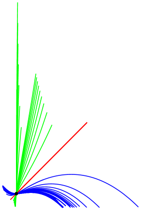
(a) Solution curves with $(U(0),V(0))$ fixed.

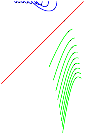
(b) Solution curves with $(U^{\prime}(0),V^{\prime}(0))$ fixed.

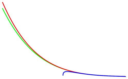
(c) Volume growth for selected solutions.

Figure 1: A collection of “planar solutions” satisfying $a=0=b$. The solution curves are given in terms of $t\mapsto(U(t),V(t))$ whilst the volume growth refers to $t\mapsto\sqrt{-\lambda(t)}$.

More precisely, in the case $U(0)=V(0)$, the normalisation forces $Q^{\prime}(0)$, written as $(x,y)=(U^{\prime}(0),V^{\prime}(0))$, to lie on the curve

$$x(x+y)^{2}=-2\sqrt{3},$$ (21)

which has two branches separated by the line $x+y=0$. One branch corresponds to positive-definite metrics, including the nearly-Kähler solution

$$x=y=\nu,\quad\hbox{where}\quad\nu=-3^{1/6}/2^{1/3}=-0.953\ldots$$ (22)

The ABC metrics are those for which $\nu<x<0$, and appear on the top left of the nearly-Kähler line in Figure 1(a), in green in the coloured version.

When $U(0)\neq V(0)$, the nearly-Kähler solution is excluded. Nevertheless, the overall picture remains valid, meaning one branch of the normalisation curve corresponds to positive-definite metrics, and this branch itself has two half pieces, one corresponding to ABC curves and one to the other solutions.

In the trace-free case, $a=0=b$, all solutions degenerate at a point $t_{0}$. The ABC solutions are “half complete”, meaning that away from the degeneration they are complete in one direction of time. (See Apostolov-S:G2 ; Chiossi-F:G2 for other examples of half-complete $\mathrm{G}_{2}$-metrics). The other solutions reach another degeneracy point $t_{1}$ in finite time. The singularity at $t_{0}$ cannot be resolved. In particular, it is not possible to find complete $\mathrm{G}_{2}$-metrics. One way to circumvent this issue is to consider flow solutions for which $[\gamma]\neq 0$; solutions of this form include the metrics discovered by Brandhuber et al Brandhuber-al:G2 .

Three-function ansatz.

Now, turning to “less symmetric” $\mathrm{G}_{2}$-metrics, we consider for solutions in $\mathcal{H}_{0}$ with $Q$ of the (generic) form:

$$Q(t)=\operatorname{diag}(-U(t)-V(t)-W(t),U(t),V(t),W(t)),$$

where $U,V,W$ are smooth functions on an interval $I\subset\mathbb{R}$. A solution of (10) is then uniquely specified by the sextuple

$$(U(0),V(0),W(0),U^{\prime}(0),V^{\prime}(0),W^{\prime}(0)).$$

As in the case of planar solutions, we have solved the flow equations for a large number of initial conditions. In contrast with the planar case, we have not been able to find metrics with one stabilising directions as $t\to\pm\infty$.

We shall confine our presentation to the class of solutions with the same initial point

$$(U(0),V(0),W(0))=(1,1,1)$$

as the nearly-Kähler solution, but with varying velocity vector

$$(x,y,z)=(U^{\prime}(0),V^{\prime}(0),W^{\prime}(0)).$$ (23)

Similar to the planar case, the flow lines are governed by the normalization condition, and (21) is replaced by the cubic surface

$$(x+y)(x+z)(y+z)=-4\sqrt{3}.$$ (24)

The asymptotic planes corresponding to the vanishing of $x+y,\,x+z,\,y+z$ separate the surface into four hyperboloid-shaped components, and only the one with all factors negative is relevant to our study of positive-definite metrics with holonomy $\mathrm{G}_{2}$. The nearly-Kähler solution $x=y=z=\nu$ (cf. (22)) corresponds to its centre point.

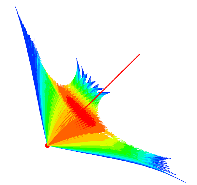
(a) Side view with diagonal nearly-Kähler line.

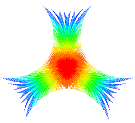
(b) Looking down the line.

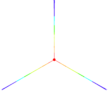
(c) Planar ABC solutions.

Figure 2: Families of space curve solutions satisfying $a=0=b$. The solution curves are given in terms of $t\mapsto(U(t),V(t),W(t))$.

Families of solutions are shown in Figure 2 which, like those in Figure 1, were plotted using Mathematica and the command NDSolve. To obtain the curves, it was convenient to further reduce attention to the case in which $x,y,z$ are all negative. The corresponding subset of (24) is now a curved triangle $\mathscr{T}$ with truncated vertices. By issuing a plotting command for $\mathscr{T}$, we obtained an abundant sample of mesh points to feed into (23) as initial values. One can then regard each curve as the continuing trajectory of a particle launched towards a point of $\mathscr{T}$, which fits in close to the apex of Figure 2(a).

All the solutions, apart from the central nearly-Kähler one, are new. They tend to have shrinking directions, causing the volume growth to slow down. The $5250$ solution curves in Figure 2(a) are plotted for the range $-0.97\leqslant t\leqslant 0$ since many develop singularities close to $t=-1$ (and close to $t=0.2$ though positive $t$ is not shown). In the coloured “cocktail umbrella” picture, they are separated into groups distinguished by the value of the function $x^{2}+y^{2}+z^{2}$ of the initial condition, with the nearly-Kähler line $x=y=z$ and its close neighbours in red. Solutions resulting from one of the coordinates being positive can be short-lived in comparison to the others, leading to less coherent plots, and this is why they are absent.

The view looking down the nearly-Kähler line from a point $(u,u,u)$ with $u\gg 1$ is shown in Figure 2(b). The $\mathbb{Z}/{3\mathbb{Z}}$ symmetry obtained by permuting the coordinates is evident. The splitting behaviour at the three “ends” is to some extent artificial, reflecting as it does the truncation that has resulted from our decision to restrict attention to the negative octant.

The ABC two-function solutions of Figure 1(a) in the previous subsection arise when two of $x,y,z$ coincide and assume a common value greater than $\nu$. The projection of these planar curves orthogonal to the nearly-Kähler line can be seen in Figure 2(c). Computations confirm that, unlike the generic curves of Figure 2(b) emanating from $(1,1,1)$, these can be extended for all $t\to-\infty$.

In addition to the solutions in $\mathcal{H}_{0}=\mathcal{H}_{(0,0)}$, we have investigated solutions in $\mathcal{H}_{(1,-1)}$. Regarding the asymptotic behaviour of the associated $\mathrm{G}_{2}$-metrics, the overall picture appears not dissimilar to the one we have described by deforming the nearly-Kähler velocity. Taking account also of the numerical analysis in Cvetic-al:G2-Spin7 , we conjecture that the only solutions that can be extended for $t\to-\infty$ or $t\to\infty$ lie in a plane.

Acknowledgements.

Both authors thank Mark Haskins for discussions that helped initiate this research, and in particular for bringing Hengesbach:phd to their attention. The first author gratefully acknowledge financial support from the Danish Council for Independent Research, Natural Sciences.

Thomas Bruun Madsen and Simon Salamon

Department of Mathematics, King’s College London,
Strand, London WC2R 2LS, United Kingdom.

E-mail: thomas.madsen@kcl.ac.uk, simon.salamon@kcl.ac.uk

References

• (1) V. Apostolov, S. Salamon, Kähler reduction of metrics with holonomy $\mathrm{G}_{2}$. Comm. Math. Phys. 246 (2004), no. 1, 43–61.
• (2) M. Atiyah, J. Maldacena, C. Vafa, An M-theory flop as a large N duality. Strings, branes, and M-theory. J. Math. Phys. 42 (2001), no. 7, 3209–3220.
• (3) C. Bär, Real Killing spinors and holonomy. Comm. Math. Phys. 154 (1993), no. 3, 509–521.
• (4) L. Bedulli, L. Vezzoni, The Ricci tensor of $\mathrm{SU}(3)$-manifolds. J. Geom. Phys. 57 (2007), no. 4, 1125–1146.
• (5) A. Brandhuber, $\mathrm{G}_{2}$ holonomy spaces from invariant three-forms. Nuclear Phys. B 629 (2002), no. 1-3, 393–416.
• (6) A. Brandhuber, J. Gomis, S. Gubser, S. Gukov, Gauge theory at large N and new $\mathrm{G}_{2}$ holonomy metrics. Nuclear Phys. B 611 (2001), no. 1-3, 179–204.
• (7) R. Bryant, Non-embedding and non-extension results in special holonomy. The many facets of geometry, 346–367, Oxford University Press, Oxford, 2010.
• (8) R. Bryant, S. Salamon, On the construction of some complete metrics with exceptional holonomy. Duke Math. J. 58 (1989), no. 3, 829–850.
• (9) J.-P. Butruille, Espace de twisteurs d’une variété presque hermitienne de dimension 6. Ann. Inst. Fourier (Grenoble) 57 (2007), no. 5, 1451–485.
• (10) J.-P. Butruille, Homogeneous nearly Kähler manifolds. Handbook of pseudo-Riemannian geometry and supersymmetry, 399–423, IRMA Lect. Math. Theor. Phys., 16, Eur. Math. Soc., Zürich, 2010.
• (11) E. Calabi, Construction and properties of some 6-dimensional almost complex manifolds. Trans. Amer. Math. Soc. 87 1958 407–438.
• (12) S. Chiossi, A. Fino, Conformally parallel $\mathrm{G}_{2}$ structures on a class of solvmanifolds. Math. Z. 252 (2006), no. 4, 825–848.
• (13) S. Chiossi, S. Salamon, The intrinsic torsion of SU(3) and $\mathrm{G}_{2}$ structures. Differential geometry, Valencia, 2001, 115–133, World Sci. Publ., River Edge, NJ, 2002.
• (14) Z. Chong, M. Cvetič, G. Gibbons, H. Lü, C. Pope, P. Wagner, General metrics of $\mathrm{G}_{2}$ holonomy and contraction limits. Nuclear Phys. B 638 (2002), no. 3, 459–482.
• (15) D. Conti, SU(3)-holonomy metrics from nilpotent Lie groups. arXiv:1108.2450 [math.DG].
• (16) M. Cvetič, G. Gibbons, H. Lü, C. Pope, Supersymmetric M3-branes and $\mathrm{G}_{2}$ manifolds. Nuclear Phys. B 620 (2002), no. 1-2, 3–28.
• (17) M. Cvetič, G. Gibbons, H. Lü, C. Pope, A $\mathrm{G}_{2}$ unification of the deformed and resolved conifolds. Phys. Lett. B 534 (2002), no. 1-4, 172–180.
• (18) M. Cvetič, G. Gibbons, H. Lü, C. Pope, Cohomogeneity one manifolds of $\mathrm{Spin}(7)$ and $\mathrm{G}_{2}$ holonomy. Phys. Rev. D (3) 65 (2002), no. 10, 106004, 29 pp.
• (19) M. Cvetič, G. Gibbons, H. Lü, C. Pope, Orientifolds and slumps in $\mathrm{G}_{2}$ and Spin(7) metrics. Ann. Physics 310 (2004), no. 2, 265–301.
• (20) A. Dancer, McKenzie Wang, Painlevé expansions, cohomogeneity one metrics and exceptional holonomy. Comm. Anal. Geom. 12 (2004), no. 4, 887–926.
• (21) A. Dancer, McKenzie Wang, Superpotentials and the cohomogeneity one Einstein equations. Comm. Math. Phys. 260 (2005), no. 1, 75–115.
• (22) J. Eschenburg, McKenzie Wang, The initial value problem for cohomogeneity one Einstein metrics. J. Geom. Anal. 10 (2000), no. 1, 109–137.
• (23) E. Ferapontov, B. Huard, A. Zhang, On the central quadric ansatz: integrable models and Painlevé reductions. J. Phys. A 45 (2012), no. 19, 195204, 11 pp.
• (24) M. Fernández, A. Gray, Riemannian manifolds with structure group $\mathrm{G}_{2}$. Ann. Mat. Pura Appl. (4) 132 (1982), 19–45 (1983).
• (25) N. Hitchin, Stable forms and special metrics. Global differential geometry: the mathematical legacy of Alfred Gray (Bilbao, 2000), 70–89, Contemp. Math., 288, Amer. Math. Soc., Providence, RI, 2001.
• (26) E. Lerman, R. Montgomery, R. Sjamaar, Examples of singular reduction. Symplectic geometry, 127–155, London Math. Soc. Lecture Note Ser., 192, Cambridge Univ. Press, Cambridge, 1993.
• (27) W. Reichel, Über die Trilinearen Alternierenden Formen in 6 und 7 Veränderlichen, Dissertation, Greifswald, (1907).
• (28) F. Reidegeld, Exceptional holonomy and Einstein metrics constructed from Aloff-Wallach spaces. Proc. Lond. Math. Soc. 102, no. 6, 1127–1160 (2011).
• (29) R. Reyes Carrión, A generalization of the notion of instanton. Differential Geom. Appl. 8 (1998), no. 1, 1–20.
• (30) S. Salamon, Riemannian geometry and holonomy groups. Pitman Research Notes in Mathematics Series, 201. Longman Scientific & Technical, Harlow; copublished in the United States with John Wiley & Sons, Inc., New York, 1989. ISBN: 0-582-01767-X.
• (31) F. Schulte-Hengesbach, Half-flat structures on Lie groups. PhD thesis (2010), Hamburg.
• (32) R. Westwick, Real trivectors of rank seven. Linear and Multilinear Algebra 10 (1981), no. 3, 183–204.