Radiative cooling implementations in simulations of primordial star formation

Abstract

We study the thermal evolution of primordial star-forming gas clouds using three-dimensional cosmological simulations. We critically examine how assumptions and approximations made in calculating radiative cooling rates affect the dynamics of the collapsing gas clouds. We consider two important molecular hydrogen cooling processes that operate in a dense primordial gas; ${\rm H_{2}}$ line cooling and continuum cooling by ${\rm H_{2}}$ collision-induced emission. To calculate the optically thick cooling rates, we follow the Sobolev method for the former, whereas we perform ray-tracing for the latter. We also run the same set of simulations using simplified fitting functions for the net cooling rates. We compare the simulation results in detail. We show that the time- and direction-dependence of hydrodynamic quantities such as gas temperature and local velocity gradients significantly affects the optically thick cooling rates. Gravitational collapse of the cloud core is accelerated when the cooling rates are calculated by using the fitting functions. The structure and evolution of the central pre-stellar disk are also affected. We conclude that physically motivated implementations of radiative transfer are necessary to follow accurately the thermal and chemical evolution of a primordial gas to high densities.

1 Introduction

The first stars fundamentally transform the early universe by emitting the first light and also by synthesizing and dispersing the first heavy elements. They initiate cosmic reionization, and set the scene for the subsequent formation of the first galaxies (see Bromm & Yoshida (2011) for a review). Understanding how and when the first stars were formed is one of the important goals of modern astronomy.

There has been a significant progress over the past years in the theoretical studies on the first stars. With the currently available computer power, one can perform an ab initio simulation of the first star formation in substantial details (see Bromm et al. (2009) for a review). Yoshida et al. (2008) studied the formation of a primordial protostar in a proper cosmological context. Turk et al. (2009) showed that a primordial gas cloud can fragment into multiple clumps by the action of the rotation and turbulence in the cloud. Clark et al. (2011) and Greif et al. (2011) used sink-particle techniques to follow the evolution of the accretion disk around a primordial protostar for hundreds years. It was shown that the circumstellar disk around a protostar becomes gravitationally unstable to form multiple protostars. Unfortunately, these simulations could not be run long enough to obtain the solid prediction for multiplicity and for the characteristic mass of the first stars. Including the so-called proto-stellar feedback effects is important to determine the mass of the first stars (McKee & Tan, 2008; Stacy et al., 2012). Recently, Hosokawa et al. (2011) performed radiation-hydrodynamical calculations to show that the self-regulating proto-stellar feedback halts the growth of a primordial protostar when its mass is several tens of solar-masses. It has become possible to follow the entire evolution of a primordial protostar to the main-sequence and thus to discuss rigorously important issues such as the characteristic mass of the first stars.

There still remain a few uncertainties in these theoretical studies on primordial star formation. For example, some of the important chemical reaction rates in a pre-stellar gas are not known to good accuracies (Glover, 2008). Most importantly, the three-body hydrogen molecule formation rate is poorly determined, which leaves substantial uncertainties in the thermal evolution of a pre-stellar gas at high densities (Turk et al., 2011). Calculating radiative cooling rates at such high densities, where the gas is optically thick, is essentially a radiative transfer problem. Previous studies adopt two methods to solve this problem. Fitting functions are proposed by Ripamonti & Abel (2004) which describes the net cooling rate as a function of the local density based on the result of a fully one-dimensional (1D) radiative transfer calculation. The other method adopts the large-velocity gradient approach, the so-called Sobolev method (Yoshida et al., 2006; Clark et al., 2011; Hosokawa et al., 2011). Similar methods have been used to follow the gas evolution at even higher densities (Ripamonti & Abel, 2004; Yoshida et al., 2007, 2008). It is important to examine whether or not the different implementations of radiative cooling calculations produce significantly different results.

In this paper, we critically examine whether or not implementations of the optically-thick radiative cooling affect the evolution of a primordial gas cloud. To this end, we run a set of three-dimensional (3D) cosmological hydrodynamical simulations. We explicitly compare the results obtained from the simulations and study the structure of the gas cloud in detail.

The rest of the paper is organized as follows. In Section 2, we describe the main physical processes in a primordial gas cloud evolution. There, we also describe the calculation methods of the net cooling rates. The simulation settings and computational methods are given in Section 3. Section 4 shows results of the cosmological simulations. We summarize the results and give concluding remarks in Section 5.

2 Thermal evolution of a primordial gas cloud

A gravitationally contracting primordial gas evolves roughly isothermally. Since the onset of run-away collapse, the temperature rises only a factor of about ten whereas the density increases over 16 orders of magnitudes (Palla et al., 1983; Omukai & Nishi, 1998). In a primordial gas, the main coolant is hydrogen molecules ($\rm{H_{2}}$). There are two important regimes where radiative transfer effects become important. One is at densities $10^{8}\ {\rm cm^{-3}}\mathrel{\hbox to0.0pt{\raise 2.20013pt\hbox{$<$}\hss}{\lower 2.20013pt\hbox{$\sim$}}}n_{\rm H}\mathrel{\hbox to0.0pt{\raise 2.20013pt\hbox{$<$}\hss}{\lower 2.20013pt\hbox{$\sim$}}}10^{14}\ {\rm cm^{-3}}$, where ${\rm H_{2}}$ line cooling is dominant and the cloud core cools and condenses rapidly. Then the cloud core becomes optically-thick to ${\rm H_{2}}$ lines. It is known that the chemo-thermal instability can be triggered in this phase (Sabano & Yoshii, 1977; Silk, 1983). The other is at densities $10^{14}\ {\rm cm^{-3}}\mathrel{\hbox to0.0pt{\raise 2.20013pt\hbox{$<$}\hss}{\lower 2.20013pt\hbox{$\sim$}}}n_{\rm H}\mathrel{\hbox to0.0pt{\raise 2.20013pt\hbox{$<$}\hss}{\lower 2.20013pt\hbox{$\sim$}}}10^{17}\ {\rm cm^{-3}}$, where the gas is nearly opaque to ${\rm H}_{2}$ line photons but cooling by the collision-induced emission (CIE) becomes efficient.

In order to compute the net radiative cooling rate in the two regimes, we need to compute the opacity for photons in a broad energy range. In principle, the gas opacity depends on a number of physical quantities such as the local gas density, temperature, and velocities.

2.1 ${\rm H_{2}}$ line cooling

When the gas density exceeds ${\rm n_{H}}\sim 10^{8}\ {\rm cm}^{-3}$, rapid three-body reactions of H₂ formation convert nearly all the hydrogen atoms into hydrogen molecules. Then H₂ line cooling becomes highly efficient. As the gas cloud condenses, however, the gas cloud core becomes opaque to H₂ lines. Then the H₂ line cooling rate is calculated as

$$\Lambda_{\mathrm{H_{2},thick}}=\sum_{u,l}h\nu_{ul}\ \beta_{{\rm escape},ul}\ A_{ul}\ n_{u}\ ,$$ (1)

where $h\nu_{ul}$ is the energy difference between the upper level $u$ and the lower level $l$, $\beta_{\mathrm{escape},ul}$ is the escape probability for a photon without absorption, $A_{ul}$ is the Einstein coefficient for the spontaneous transition, and $n_{u}$ is the number density of the hydrogen molecule in the upper level $u$. To calculate the escape probability $\beta_{\rm escape}$, we evaluate the opacity for each H₂ line as

$$\tau_{lu}=\alpha_{lu}L\ ,$$ (2)

where $\alpha_{lu}$ is the absorption coefficient for the transition from $l$ to $u$ level. Calculating the characteristic absorption length scale, $L$, is the remaining task. To this end, we adopt the Sobolev method. The Sobolev length along a line of sight is defined as

$$L_{r}={{v_{{\rm thermal}}}\over{|dV_{r}/dr|}}\ ,$$ (3)

where $v_{\mathrm{thermal}}=(kT/m_{\mathrm{H}})^{1/2}$ is the typical thermal velocity of the hydrogen molecules and $V_{r}$ is the fluid velocity in the direction. The escape probability for a spherical cloud is given by

$$\beta_{\mathrm{escape}}={{1-\exp(-\tau)}\over{\tau}}\ ,\ \tau=\alpha L_{r}\ .$$ (4)

We compute the Sobolev length and the escape probability in three orthogonal directions and use the average value of them to calculate the net cooling rate.

The above method requires the evaluation of the optical depths for a few hundred molecular lines, and thus is computationally costly. Ripamonti & Abel (2004) propose a fitting formula for the optically-thick cooling rate based on the result of 1D radiative transfer simulations. It is given by

$$\Lambda_{{\rm H}_{2},{\rm thick}}=\Lambda_{{\rm H}_{2},{\rm thin}}\times\min\left[1,\left(\frac{n}{8\times 10^{9}\ {\rm cm}^{-3}}\right)^{-0.45}\right]\ .$$ (5)

Note that the simple function depends only on the local gas density. We use the formula as an alternative method to compute the net cooling rate.

2.2 Collision-induced emission cooling

At densities greater than $n_{\rm H}\sim 10^{14}\ {\rm cm^{-3}}$, hydrogen molecules collide so frequently that each collision pair temporarily induces an electric dipole and either molecule makes an energy transition by emitting a photon. This process is known as collision-induced emission (CIE), which acts as an efficient radiative cooling process at such high densities. The resulting emission spectrum appears essentially as continuum radiation. We use the collision cross-sections of Jorgensen et al. (2000), Borysow et al. (2001), and Borysow (2002).

At even higher densities $n_{\rm H}>10^{16}\ {\rm cm^{-3}}$, the gas cloud becomes opaque to the continuum emission. We use the Planck opacity table (Lenzuni et al., 1991) to calculate the gas opacity and the resulting radiative cooling rate. By noting that the net energy transfer rate should scale as $\Lambda\propto 1/(1+\tau)$ for small $\tau$, whereas it scales as $\Lambda\propto 1/{\tau}^{2}$ for large $\tau$, we assume a simple form of double power-law

$$f=\frac{1}{[1+\tau(n,T)][1+(\tau(n,T)/10)]}$$ (6)

as the “efficiency” factor of the CIE cooling. Although the particular functional form is somewhat ad hoc, it reproduces well the net cooling rate that is obtained from more detailed radiative transfer calculations (Omukai & Nishi, 1998; Yoshida et al., 2008). Note that we explicitly write as $\tau=\tau(n,T)$ to express that the local opacity depends on the gas density and temperature. In practice, we compute the opacity along a line-of-sight by the integral

$$\tau=\int\kappa(\rho,T)\rho\;{\rm d}l\ ,$$ (7)

where $\kappa$ is the absorption coefficient and $\rho$ is the local gas density. In order to take the cloud geometry and structure into account, we take the mean of the efficiency factors in three orthogonal directions (see equation [6]),

$$f_{{\rm mean}}=\frac{f_{\rm x}+f_{\rm y}+f_{\rm z}}{3}\ .$$ (8)

Then the CIE cooling rate is calculated as

$$\Lambda_{\mathrm{CIE,thick}}=\Lambda_{\mathrm{CIE,thin}}\times f_{{\rm mean}}\ .$$ (9)

A simple continuum opacity model is also proposed by Ripamonti & Abel (2004), which is given by a function of the local gas density $n_{{\rm H}_{2}}$ as

$$\Lambda_{{\rm CIE},{\rm thick}}=\Lambda_{{\rm CIE},{\rm thin}}\times\min\left[1,\frac{1-e^{-{\tau}_{\rm CIE}}}{{\tau}_{\rm CIE}}\right]\ ,$$ (10)

where

$${\tau}_{\rm CIE}=\left(\frac{n_{{\rm H}_{2}}}{7\times 10^{15}\ {\rm cm^{-3}}}\right)^{2.8}\ .$$ (11)

We compare the runs with the above two methods of computing the CIE cooling rate. (as equation [9] and [10]).

3 Numerical Simulations

We use the parallel $N$-body/Smoothed Particle Hydrodynamics (SPH) solver $GADGET$-2 (Springel, 2005) in its version suitably adopted for the primordial star formation. We solve chemical rate equations for fourteen species of primordial species (${\rm e^{-}}$, ${\rm H}$, ${\rm H^{+}}$, ${\rm He}$, ${\rm He^{+}}$, ${\rm He^{++}}$, ${\rm H_{2}}$, ${\rm H_{2}^{+}}$, ${\rm H^{-}}$, ${\rm D}$, ${\rm D^{+}}$, ${\rm HD}$, ${\rm HD^{+}}$, ${\rm HD^{-}}$). The reactions and rates are summarized in Yoshida et al. (2006, 2007). We adopt the $\Lambda$-Cold Dark Matter ($\Lambda$-CDM) cosmology. The cosmological parameters are based on the seven-year WMAP results (Larson et al., 2011); ${\Omega}_{\Lambda}=0.734,\ {\Omega}_{m}=0.236,\ {\Omega}_{b}=0.0449$, and $H_{0}=71.0\ \mathrm{km\ s^{-1}\ Mpc^{-1}}$. The normalization of the power spectrum is set to be ${\sigma}_{8}=2.0$ such that structure forms early in the small simulation volume. All simulations are initialized at $z_{\rm ini}=99$.

We use the zoom-in re-simulation techniques to achieve a large dynamic range. First, we run a cosmological simulation to locate a star-forming halo which is later re-simulated with a higher resolution. The comoving box size of this parent simulation is $50\ {\rm kpc\ h^{-1}}$ on a side. In the zoomed region, the initial particle masses are $m_{\rm gas}=2.04\times 10^{-3}\ M_{\odot}$ and $m_{\rm DM}=1.01\times 10^{-2}\ M_{\odot}$, respectively.

We run each of the zoomed simulations first to the point where the central density reaches $n_{\rm cen}=10^{8}\ {\rm cm^{-3}}$. Then, to calculate the gas collapse further, we use the particle split method of Kitsionas & Whitworth (2002) to achieve a higher mass resolution. We do this refinement progressively such that a local Jeans length is always resolved by 10 times the local SPH smoothing length. By using this technique, we achieve a mass resolution of $m_{\rm gas}=4\times 10^{-6}\ M_{\odot}$ at the last output time. We stop the simulations when the central density reaches $n_{\rm cen}=10^{17}\ {\rm cm^{-3}}$.

4 Results

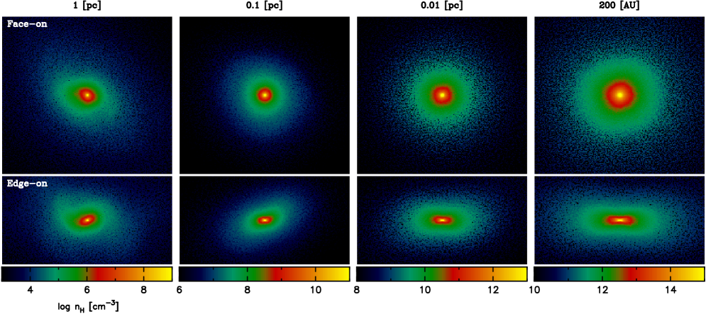
Figure 1: Projected density distribution for Run A, which shows a flattened disk-like structure. Face-on views (top panels) and edge-on views (bottom panels) in a volume of, from left to right, $1$, $10^{-1}$, $10^{-2}$, and $10^{-3}$ pc $\sim 200$ AU on a side, respectively.

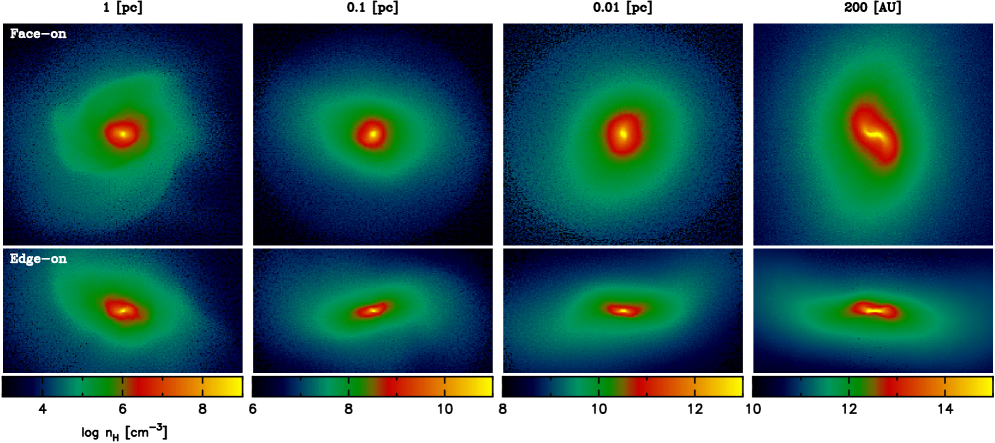
Figure 2: As for Figure 1, but for Run B.

To examine the properties of star-forming halos, we choose two realizations as characteristic cases, Run A and B. Run A forms a disk-like structure inside the collapsing gas cloud, whereas Run B shows elongated structure and eventually develops S-shape arms (see the top panels in Figures 1 and 2). The bottom panels show, in both cases, the central sub-parsec region is significantly flattened. The non-spherical structures likely yield direction-dependence of both line and continuum opacities.

In the following subsections, we first compare the opacity models for H₂ line cooling. Then we examine differences in the CIE cooling phase. We have already mentioned the importance of the three-body molecular hydrogen formation rate (Turk et al., 2011). We examine the effect of varying the three-body reaction rate at the end of this section.

4.1 ${\rm H_{2}}$ line cooling

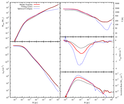
Figure 3: Radial profiles of various quantities for Run A. Five panels show the enclosed mass, temperature, radial velocity, gas number density, and gas mass accretion rate, in the clockwise order starting from the top-left. The solid line shows the result with the 3D ${\rm H_{2}}$ line opacity calculation (Sobolev method), the dotted line is for the run with the fitting function and the dashed line is for a spherical collapse calculation with 3D set-up.

Figure 3 shows the radial profiles of five physical quantities for Run A when the central density is $n_{\rm H}\sim 10^{14}\ {\rm cm^{-3}}$. At this time, the central part is nearly completely opaque to H₂ line emission. The solid line shows the result from the run with the 3D opacity calculation (Sobolev method, equation [1]) and the dotted line is for the run with the fitting opacity formula (equation [5]). We see significant differences in the temperature, radial velocity, and accretion rate profiles.

Because the photon escape probability depends on the local velocity gradient (see equation [3]), the line cooling rate can be large if the velocity gradient is large in the dense cloud core. The radial infall velocity is critically affected by the degree of rotation of the collapsing cloud. Star-forming clouds in a cosmological simulation generically have finite initial angular momenta and thus they spin up gradually as they collapse gravitationally. The radial infall velocity, $V_{r}$, and the velocity gradient, $dV_{r}/dr$, in such rotating gas clouds are smaller than realized in spherically symmetric collapse. Thus the escape probability in the cosmological simulation is smaller than the fitting formula predicts.

In order to investigate further the difference in the escape probability, we perform a spherical collapse simulation with 3D set-up. We follow gravitational collapse of a super-critical Bonnor-Ebert sphere having a mass of $\sim 1000\ M_{\odot}$. For this run, we calculate the H₂ line opacity using the Sobolev method. The results are shown in Figure 3 (dashed line in each panel). Clearly, the radial velocity of the run is larger than that of our cosmological simulation Run A, which has a substantial degree of rotation. This is the major source of the differences in the line escape probability and in the cooling rate, as shown in Figure 4.

The left panel of Figure 4 shows the escape probability of H₂ line photons as a function of the gas density. We show three snapshots for the mean profiles (solid lines) when the central density is $n_{\rm cen}=10^{10},\ 10^{12}$, and $10^{14}\,{\rm cm}^{-3}$. The escape probability calculated by our 3D treatment is smaller than the fitting formula (dotted line) most of the time. The difference is as large as a factor of ten at the densest part. The fitting formula over-estimates the net cooling rate. This is easily understood by the collapse speed of the spherically symmetric calculation.

Next, let us consider the direction-dependence of the escape probability. In the left panel of Figure 4, we plot the escape probability in the direction along $x-,\ y-,$ and $z$-axes (long-dashed, short-dashed, and dot-dashed lines). We configure the coordinate such that the $z$-direction is aligned to the angular momentum vector of the central cloud core . The escape probability is large along the $z$-direction. Thus, physically, line photons preferentially escape in perpendicular directions to the flattened cloud core.

It is important to note that the difference (or mis-estimate) in the cooling rate critically affects the collapse dynamics. The right panel of Figure 4 shows the time evolution of the central density since the central density reaches $n_{\rm cen}=10^{8}\ {\rm cm}^{-3}$. In the run with the fitting formula, the cloud core collapses earlier by $\sim 20,000$ years, i.e., the gravitational collapse is accelerated because of the “efficient” cooling.

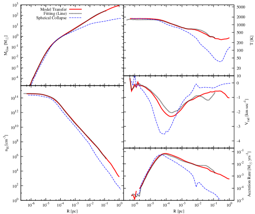
Figure 5: As for Figure 3 but for Run B.

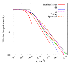
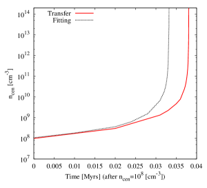
Figure 6: As for Figure 4 but for Run B.

Figures 5 and 6 show the same results for Run B, which has a spiral structure. The overall evolutionary trend is quite similar to Run A. Clearly, the importance of radiative transfer effects is not particular to the configuration of Run A. The differences in the radial profiles of Run B are understood similarly to Run A as explained in the present section. We conclude that the multi-dimensional treatment for the radiative cooling is important to follow the thermal evolution and the gravitational collapse accurately.

4.2 ${\rm H_{2}}$ collision-induced emission cooling

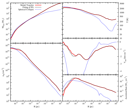
Figure 7: Radial profiles of various quantities for Run B in the high density regime where CIE cooling is important. Five panels show the enclosed mass, temperature, radial velocity, gas number density, and mass accretion rate, in the clockwise order starting from the top-left. The solid line is for the result with the 3D ${\rm H_{2}}$ CIE opacity calculation, the dotted line is for the run with the fitting function and the dashed line is for a spherical collapse calculation with 3D treatments.

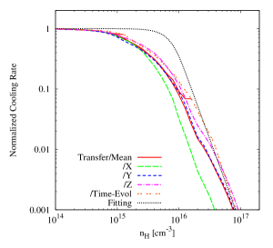
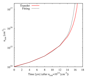
Figure 8: Left panel: The net cooling rate by ${\rm H_{2}}$ CIE emission for Run B. The long-dashed, short-dashed, and dot-dashed lines show the three orthogonal components ($x$, $y$, and $z$) when the central density is $n_{\rm cen}=10^{17}\ {\rm cm^{-3}}$. The solid lines show the mean values of them at $n_{\rm cen}=10^{15},\ 10^{16}$, and $10^{17}\ {\rm cm^{-3}}$. The double-dotted line is the time-evolution of the central part. The dotted line shows the fitting function given by equation (10). Right panel: The time evolution of the central density. The horizontal axis is the elapsed time after the central density reaches $\sim 10^{14}\ {\rm cm^{-3}}$.

Next, we discuss the thermal evolution through the phase where CIE cooling is important. In this subsection, we primarily discuss the results of Run B. The radial profiles when the central density is $n_{\rm cen}\sim 10^{17}\ {\rm cm}^{-3}$ are shown in Figure 7. We also plot the normalized cooling rate, the efficiency factor $f=\Lambda_{\mathrm{CIE,thick}}/\Lambda_{\mathrm{CIE,thin}}$ and the time evolution of the central density in Figure 8.

The left panel of Figure 8 shows similar features to the case of ${\rm H_{2}}$ line opacity discussed in the previous section. We a significant direction-dependence of the escape probability. The fitting formula over-estimates the net cooling rate compared with the run with our 3D opacity treatment. The difference in the net cooling rate becomes as large as a factor of 5 at $n_{\rm cen}\sim 5\times 10^{15}\ {\rm cm}^{-3}$. The gas collapses faster with the fitting formula for the opacity calculation. However, the difference in the resulting collapse time is not very large (see the right panel of Figure 8). The time difference is only about 1 year at the end of the calculations.

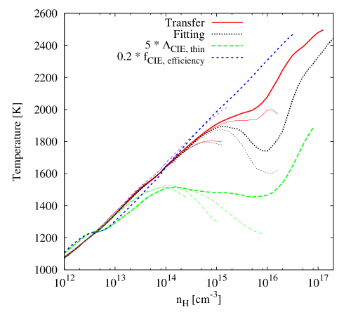
Figure 9: Thermal evolution in the temperature - density plane for Run B. We plot the simulation results with our 3D radiative transfer treatment (solid), with the fitting opacity function (dotted), with a increased CIE cooling rate (long-dashed), and with a reduced CIE escape probability (short-dashed). The thick lines show the final output time and the the thin lines are for the results at earlier phases.

It is worth pursuing the reason why the collapse proceeds similarly in the two cases despite the large difference in the net cooling rate in the relevant regime $n_{\rm H}\sim 10^{15}-10^{16}\ {\rm cm}^{-3}$. To this end, we perform two additional calculations for Run B. One is run with an artificially increased CIE cooling rate as $\Lambda_{\rm CIE}\to 5\times\Lambda_{\rm CIE}$ whereas the other is run with the reduced efficiency factor $f_{\rm mean}\to 0.2\times f_{\rm mean}$. The other configurations are identical to Run B, and the opacity calculations are also done using 3D ray-tracing. Therefore, we expect that the two runs clarify the impact of enhanced/reduced CIE cooling. The results are shown in Figure 9. In the case with the increased cooling rate, the collapsing gas evolves on a lower temperature track (the long-dashed line in Figure 9), as is naively expected from the enhanced cooling rate. Clearly, the cooling rate itself directly affects the gas temperature in this regime. On the other hand, the effect of decreasing the efficiency factor appears relatively small (the short-dashed line). The cloud evolves on a slightly higher temperature track, but the difference is significant only in a narrow range of density, $10^{15}<n_{\rm H}<10^{16}\ {\rm cm}^{-3}$, where the gas is collapsing rapidly. The free-fall time there is estimated to be $t_{\rm ff}\sim 1\ {\rm year}$ which is comparative to the cooling time. The core condenses quickly and becomes optically thick to the continuum photons after the central density reaches $\sim 10^{16}\ {\rm cm}^{-3}$. In the left panel of Figure 8, we also plot the time evolution of the cooling efficiency at the central part (double-dotted line). The evolution looks similar to the fitting function at the high density.

In summary, the accuracy of the continuum opacity calculation causes only minor effect on the thermal evolution. The difference in $f=\Lambda_{\mathrm{CIE,thick}}/\Lambda_{\mathrm{CIE,thin}}$ is large between the methods, but the resulting evolution is not sensitive to the details of the methods. It should be noted, however, that we have considered only a particular case in which the central core undergoes rapid run-away collapse. In other circumstances, for example in an accretion disk around a protostar where the density evolution is much slower than in the collapsing gas core that we have studied, accurate calculations of the optically-thick cooling may be more important.

4.3 Three-body ${\rm H_{2}}$ formation

It is well known that there is a large uncertainty in the reaction rate of the three-body H₂ formation

$${\rm H+H+H\to H_{2}+H}\ .$$ (12)

Because this is the dominant reaction to form hydrogen molecules at high densities ($n_{\rm H}>10^{8}\ {\rm cm^{-3}}$), an accurate reaction rate is needed to determine the chemical and thermal evolution of a primordial gas cloud. Glover (2008) summarize various rate coefficients used in the literature, which differ by a factor of 30 at the relevant temperature range. Turk et al. (2011) perform a set of hydrodynamical simulations to directly study the overall effect caused by the uncertainties in the reaction rate. They conclude that, while the difference between different realizations (gas cloud samples) is larger than that caused by the uncertainty of the three-body rate coefficient, the morphology and the collapse time of a gas cloud depend strongly on the reaction rate.

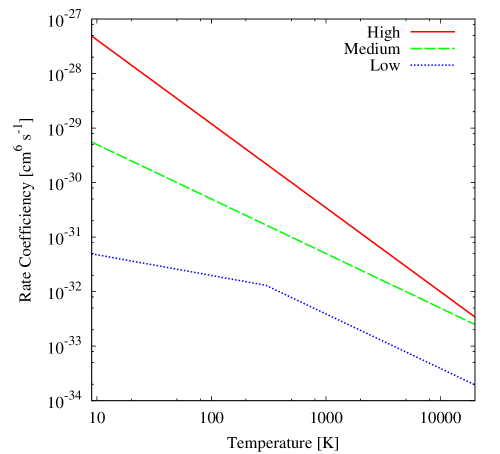
Figure 10: Three-body H₂ formation reaction rate used in the literature. The solid line (High) is the rate from Flower & Harris (2007), the dashed line (Medium) is from Palla et al. (1983), and the dotted line is from Abel et al. (2002). The rates are explicitly given in Table Radiative cooling implementations in simulations of primordial star formation.

In this section, we revisit the issue because the density range where the uncertainties are relevant is coincident with the range where the radiative transfer treatment is important, as studied in the previous sections. We are able to compare the overall differences caused by the uncertainties of the reaction rates with the differences caused by radiative transfer treatments. So far in the present paper, we have adopted the reaction rate from Palla et al. (1983) ($Medium$ case in Figure 10). We run the same simulation as Run B but with the different three-body reaction rates of Flower & Harris (2007) ($High$) and Abel et al. (2002) ($Low$), which are the largest and smallest reaction rates among those compiled by Glover (2008). The respective rates are summarized in Figure 10 and Table Radiative cooling implementations in simulations of primordial star formation.

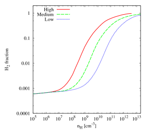
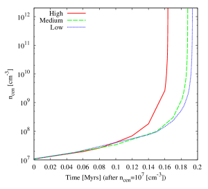
Figure 11: Left panel: Molecular fraction as a function of the gas density. Three lines show the runs with three reaction rates (see Figure 10 and Table Radiative cooling implementations in simulations of primordial star formation). Right panel: The time evolution of the central density. The horizontal axis is the elapsed time after the central density reaches $\sim 10^{7}\ {\rm cm^{-3}}$.

Figure 11 shows the simulation results with the three reaction rates. The left panel shows the H₂ fraction as a function of gas density. The density at which the cloud becomes fully-molecular differs more than a factor of 10. This is consistent with the conclusion of Turk et al. (2011). Because the molecular fraction largely determines the H₂ line cooling rate, the resulting collapse time of the cloud differs by $\Delta t\sim 30,000$ years, depending on the choice of the reaction rate. It is interesting that the time difference of the cloud collapse, $\Delta t$, is comparable to the difference caused by the choice of the opacity calculation method. The difference in the molecular fraction becomes large at $n_{\rm H}>10^{9}\ {\rm cm}^{-3}$, where the calculation of the H₂ line opacity is important (see Figure 6). Therefore, we argue that using an accurate radiative transfer method is as important as using an accurate reaction rate.

5 Discussion and Conclusion

Radiative cooling by hydrogen molecules governs the thermal evolution of a primordial star-forming gas cloud. At high densities, the cloud core becomes optically thick to both the rot-vibrational lines and collision-induced continuum. It is necessary to estimate the gas opacities in multiple directions in order to calculate the radiative cooling rates accurately. We have explicitly compared the results from several sets of simulations with different manners to calculate the optically-thick cooling rates.

When non-spherical structures develop in the central region of the cloud, photons do not escape isotropically from the dense part. Our simulations show that the gas cloud spins up as it contracts, and forms a flattened disk at the center. Then the photon escape probability not only varies with time but is also direction-dependent. Utilizing an “isotropic” fitting formula that is derived from spherically symmetric calculations over-estimates the net cooling rate and causes the cloud core to collapse fast (see Figures 4, 6, and 8). With our 3D opacity calculation, the photon escape fraction from the cloud core is always smaller than given by the fitting formula. The resulting cooling rate differs by a factor of a few to 10, depending on the exact density, temperature, and velocity structure. There is also a directional effect of the radiative transfer. In perpendicular directions to the faces of the disk-like cloud, photons can easily escape.

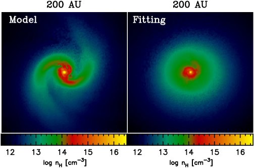
Figure 12: Projected density distributions for the same realization but with different opacity calculations at 10 years after the central density reaches $10^{18}\ {\rm cm^{-3}}$. The plotted region is $200\ {\rm AU}$ on a side. The left panel is for the result with our 3D opacity calculation, whereas the right panel is for the run with the fitting opacity for line emission.

Details of the implementation of the optically-thick radiative cooling affects the thermal and dynamical evolution of the cloud. Figure 12 shows the density distribution of two characteristic runs. We use the snapshots at 10 years after the central density reaches $n_{\rm cen}=10^{18}\ {\rm cm^{-3}}$. The left panel shows the case with our 3D radiative transfer, whereas the right panel is for the case with the fitting formulae . The latter case appears rounder and more concentrated than former, which has a spiral structure. Clearly, further detailed studies on radiative transfer effects are needed, particularly on the long-term evolution of the proto-stellar disk. The exact structure of the proto-stellar disk likely affects the disk evolution, mass accretion rate and fragmentation of the cloud (Greif et al., 2012).

A similar comparative study of radiative cooling implementations has been done by Wilkins & Clarke (2012) in the context of the present-day star formation. Interestingly, an opposite trend is found in the case of “polytropic” cooling examined by Wilkins & Clarke (2012), which is based on locally estimated opacities. They show that the polytropic cooling performs well only in spherically symmetric cases. The polytropic method over-estimates the column density, and hence underestimates the radiative cooling rate in non-spherical cases. In order to calculate radiative cooling rates in 3D simulations, it is important to take the direction-dependence of the photon diffusion into account, similarly to what we conclude in the present paper.

It is clearly advantageous to use a computational method that is fast and robust. Our method of the H₂ line transfer utilizes local velocity gradients that come with essentially no additional cost, because the velocity gradients are already computed and used in the other parts in our smoothed-particle hydrodynamics code. For continuum photons, we need to compute the column density along six (or more) directions using a costly projection method devised by Yoshida et al. (2007). In fact, the continuum opacity calculation is one of the most time consuming part in our 3D simulations. Nevertheless, we argue that it is necessary to properly take the direction-dependence into account in order to calculate the optically-thick radiative cooling rate accurately. We also note that our method is based on the so-called escape probability method, which itself is an approximation. Essentially, we assume only the densest part emits continuum photons. It is desirable to implement fully three-dimensional radiative transfer, by employing advanced methods such as flux-limited diffusion or M1-closure (e.g., Whitehouse & Bate (2004); Levemore (1984)) to follow the long-term evolution of a primordial proto-stellar system.

Hydrodynamical simulations with radiative cooling are commonly used for the study of the primordial star formation. In such simulations, it is important to use accurate methods to calculate radiative cooling rates. For example, whether or not a proto-stellar disk fragments is determined by the thermal and gravitational instability of the circumstellar gas. The disk fragmentation is an important issue which is thought to determine the multiplicity and possibly the characteristic mass of primordial stars. Our study clarifies the importance of multi-dimensional radiative processes in a primordial star-forming cloud.

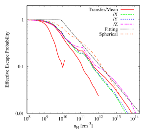
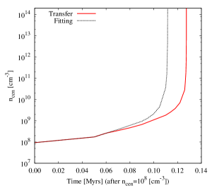
Figure 4: Left panel: The effective escape probability, $\Lambda_{\rm thick}/\Lambda_{\rm thin}$, for ${\rm H_{2}}$ line cooling for Run A. The long-dashed, short-dashed, and dot-dashed lines show the three orthogonal components ($x$, $y$, and $z$) when the central density is $n_{\rm cen}=10^{14}\ {\rm cm^{-3}}$. The solid lines show the evolution of the direction-averaged mean value at $n_{\rm cen}=10^{10},\ 10^{12}$, and $10^{14}\ {\rm cm^{-3}}$. The dotted line shows the fitting function given by equation (5). The double-dotted line indicates the result of a spherical collapse calculation with 3D treatments. Right panel: The time evolution of the central density. The horizontal axis is the elapsed time after the central density reaches $\sim 10^{8}\ {\rm cm^{-3}}$.

Table 1: Three-body H₂ formation rate

Model	${\rm Rate\ Coefficient\ (cm^{6}\ s^{-1})}$		Reference
High	$1.44\times 10^{-26}\ T^{-1.54}$		1
Medium	$5.5\times 10^{-29}\ T^{-1.0}$		2
Low	$1.14\times 10^{-31}\ T^{-0.38}$	($T$ $\leq$ 300 K)	3
	$3.9\times 10^{-30}\ T^{-1.0}$	($T$ $>$ 300 K)	3

Note. — $T$ is the gas temperature in Kelvin.

References. — (1) Flower & Harris (2007); (2) Palla et al. (1983); (3) Abel et al. (2002).

References

- Abel et al. (2002) Abel, T., Bryan, G. L. & Norman, M. L. 2002, Science, 295, 93
- Borysow (2002) Borysow, A. 2002, A&A, 390, 779
- Borysow et al. (2001) Borysow, A., Jorgensen, U. G. & Fu, Y. 2001, J. Quant. Spec. Radiat. Transf., 68, 235
- Bromm et al. (2009) Bromm, V., Yoshida, N., Hernquist, L. & McKee, C. F. 2009, Nature, 459, 49
- Bromm & Yoshida (2011) Bromm, V. & Yoshida, N. 2011, ARA&A, 49, 373
- Clark et al. (2011) Clark, P. C., Glover, S. C. O., Smith, R. J., Greif, T. H., Klessen, R. S. & Bromm, V. 2011, Science, 331, 1040
- Flower & Harris (2007) Flower, D. R. & Harris, G. J. 2007, MNRAS, 377, 705
- Glover (2008) Glover, S. C. O. 2008, in AIP Conf. Proc, 990, First Star III, ed. O’Shea, B., Heger, A. & Abel, T. (Melville, NY: AIP), 25
- Greif et al. (2012) Greif, T. H., Bromm, V., Clark, P. C., Glover, S. C. O., Smith, R. J., Klessen, R. S., Yoshida, N. & Springel, V. 2012, MNRAS, 424, 399
- Greif et al. (2011) Greif, T. H., Springel, V., White, S. D. M., Glover, S. C. O., Clark, P. C., Smith, R. J., Klessen, R. S. & Bromm, V. 2011, ApJ, 737, 75
- Hosokawa et al. (2011) Hosokawa, T., Omukai, K., Yoshida, N. & Yorke, H. W. 2011, Science, 334, 1250
- Jorgensen et al. (2000) Jorgensen, U. G., Hammer, D., Borysow, A. & Falkesgaard, J. 2000, A&A, 361, 283
- Kitsionas & Whitworth (2002) Kitsionas, S. & Whitworth, A. P. 2002, MNRAS, 330, 129
- Larson et al. (2011) Larson, D. et al. 2011, ApJS, 192, 16
- Lenzuni et al. (1991) Lenzuni, P., Chernoff, D. F. & Salpeter, E. E. 1991, ApJS, 76, 759
- Levemore (1984) Levermore, C. D. 1984, J. Quant. Spec. Radiat. Transf., 31, 149
- McKee & Tan (2008) McKee, C. F. & Tan, J. C. 2008, ApJ, 681, 771
- Omukai & Nishi (1998) Omukai, K. & Nishi, R. 1998, ApJ, 508, 141
- Palla et al. (1983) Palla, F., Salpeter, E. E. & Stahler, S. W. 1983, ApJ, 271, 632
- Ripamonti et al. (2002) Ripamonti, E., Haardt, F., Ferrara, A. & Colpi, M. 2002, MNRAS, 334, 401
- Ripamonti & Abel (2004) Ripamonti, E. & Abel, T. 2004, MNRAS, 348, 1019
- Sabano & Yoshii (1977) Sabano, Y. & Yoshii, Y. 1977, PASJ, 29, 207
- Silk (1983) Silk, J. 1983, MNRAS, 205, 705
- Springel (2005) Springel, V. 2005, MNRAS, 364, 1105
- Stacy et al. (2012) Stacy, A., Greif, T. H. & Bromm, V., 2012, MNRAS, 422, 290
- Turk et al. (2009) Turk, M. J., Abel, T. & O’Shea, B. 2009, Science, 325, 601
- Turk et al. (2011) Turk, M. J., Clark, P., Glover, S. C. O., Greif, T. H., Abel. T., Klessen, R. & Bromm, V. 2011, ApJ, 726, 55
- Yoshida et al. (2006) Yoshida, N., Omukai, K., Hernquist, L. & Abel, T. 2006, ApJ, 652, 6
- Yoshida et al. (2007) Yoshida, N., Oh, S. P., Kitayama, T. & Hernquist, L. 2007, ApJ, 663, 687
- Yoshida et al. (2008) Yoshida, N., Omukai, K. & Hernquist, L. 2008, Science, 321, 669
- Whitehouse & Bate (2004) Whitehouse, S. C. & Bate, M. R. 2004, MNRAS, 353, 1078
- Wilkins & Clarke (2012) Wilkins, D. R. & Clarke, C. J. 2012, MNRAS, 419, 3368