Abstract

The (1+1)-dimensional nonlinear boundary value problem, modeling the process of melting and evaporation of metals, is studied by means of the classical Lie symmetry method. All possible Lie operators of the nonlinear heat equation, which allow us to reduce the problem to the boundary value problem for the system of ordinary differential equations, are found. The forms of heat conductivity coefficients are established when the given problem can be analytically solved in an explicit form.

1 Introduction

It is well-known that processes of melting and evaporation of metals in the case where their surface is exposed to a powerful flux of energy are described by a nonlinear boundary value problem of the Stefan type [1, 4, 3, 2]. In the (1+1)-dimensional case the relevant boundary value problem (BVP) reads as [5, 7, 6]:

$$\frac{\partial}{\partial x}\left(\lambda_{1}(T_{1})\frac{\partial T_{1}}{\partial x}\right)=C_{1}(T_{1})\frac{\partial T_{1}}{\partial t},\ \ \ 0<S_{1}(t)<x<S_{2}(t),$$ (1)

$$\frac{\partial}{\partial x}\left(\lambda_{2}(T_{2})\frac{\partial T_{2}}{\partial x}\right)=C_{2}(T_{2})\frac{\partial T_{2}}{\partial t},\ \ \ x>S_{2}(t),$$ (2)

$$\qquad x=S_{1}(t):\lambda_{1}(T_{1})\frac{\partial T_{1}}{\partial x}=\frac{dS_{1}}{dt}H_{v}-q(t),$$ (3)

$$\qquad x=S_{1}(t):T_{1}=T_{v},$$ (4)

$$\qquad x=S_{2}(t):\lambda_{2}(T_{2})\frac{\partial T_{2}}{\partial x}=\lambda_{1}(T_{1})\frac{\partial T_{1}}{\partial x}+\frac{dS_{2}}{dt}H_{m},$$ (5)

$$\qquad x=S_{2}(t):T_{1}=T_{2}=T_{m},$$ (6)

$$\qquad x=+\infty:T_{2}=T_{0},$$ (7)

where $T_{v}$, $T_{m}$, $T_{0}$ are the known temperatures of evaporation, melting, and solid phase of metal, respectively; $\lambda_{k}$ are thermal conductivities; $C_{k}$, $H_{v}$, $H_{m}$ are specific heat values per unit volume; $q(t)$ is a function presenting the energy flux being absorbed by the metal; $S_{k}$ are the phase division boundary coordinates to be found; $\frac{dS_{k}}{dt}$ are the phase division boundary velocities; $T_{k}(t,x)$ are unknown temperature fields; and index $k=1,2$ corresponds to the liquid and solid phases, respectively.

In this BVP with moving boundaries, Eqs. (1) and (2) describe the heat transfer process in liquid and solid phases, respectively, the boundary conditions (3) and (4) present evaporation dynamics on the surface $S_{1}$, and the boundary conditions (5) and (6) are the well-known Stefan conditions on the surface $S_{2}$ dividing the liquid and solid phases. Assuming that the liquid phase thickness is considerably less than the solid phase thickness, one may use the Dirichlet condition (7). It should be stressed that we neglect the initial distribution of the temperature in the solid phase and consider the process at that stage when two phases already take place. This means that we start to describe the process at time $t=t^{*}>0$ when

$$T_{1}=T_{l}(t),\quad T_{2}=T_{s}(t),$$

where $T_{l}(t)$ and $T_{s}(t)$ are non-constant functions, which are defined by the solutions of the problem (1)–(7).

The simplest realistic case of this BVP with moving boundaries occurs under the assumption $q(t)=\mbox{const}$ when the process has a long quasistationary phase after a short transient phase for $t\in(0,t^{*})$. It means that the unknown functions $S_{1}$ and $S_{2}$ are linear with respect to the time if $t>t^{*}$ and $S_{2}-S_{1}=\mbox{const}$; therefore, the BVP (1)–(7) can be reduced to the problem for ordinary differential equations by ansatz

$$T_{1}=T_{1}(z),\quad T_{2}=T_{2}(z),\quad z=x-vt,$$

where $v=\frac{dS_{1}}{dt}=\frac{dS_{2}}{dt}>0$ is an unknown phase division boundary velocity. It turns out that the BVP obtained can be exactly solved in an implicit form; moreover, the solution is expressed in an explicit form for a wide range of functions $\lambda_{k}$ and $C_{k}$ [5, 7]. Note that the case of constant values $\lambda_{k}$ and $C_{k}$, i.e. the fact that Eqs. (1) and (2), are linear heat equations, was considered in the pioneering paper [8].

This paper is devoted to finding new reductions of the nonlinear BVP (1)–(7) to the simpler problems and to constructing their exact solutions. The main idea is to apply the classical Lie symmetry method [9, 11, 10]. In section 2, all possible Lie operators of the nonlinear heat equations (1) and (2), which allow us to reduce the problem to the BVP for an ordinary differential equation system, are found. In section 3, the forms of the coefficients arising in BVP (1)–(7) are established when the boundary value problems obtained in section 2 can be analytically solved in an explicit form and the relevant exact solutions are constructed. Application of the exact solution obtained in the case of linear basic equations (see Eqs. (1) and (2) with constant coefficients) is presented to calculate the temperature fields and phase division boundary coordinates for the parameters, which are typical for aluminium. Section 4 concludes the paper.

2 Reduction of the problem to the nonlinear BVP for the system of ODEs

It can be noted that BVP (1)–(7) can be simplified if one applies the Kirchhoff substitution

$$u=\int\limits_{0}^{T_{1}}{C_{1}(T_{1})}\,dT_{1},\quad v=\int\limits_{0}^{T_{2}}{C_{2}(T_{2})}\,dT_{2}.$$ (8)

Substituting (8) into (1)–(7) and making the relevant calculations, we arrive at the equivalent BVP of the form

$$\frac{\partial u}{\partial t}=\frac{\partial}{\partial x}\left(d_{1}(u)\frac{\partial u}{\partial x}\right),\ \ \ t>0,\ S_{1}(t)<x<S_{2}(t),$$ (9)

$$\frac{\partial v}{\partial t}=\frac{\partial}{\partial x}\left(d_{2}(v)\frac{\partial v}{\partial x}\right),\ \ \ t>0,\ x>S_{2}(t),$$ (10)

$$\qquad x=S_{1}(t):d_{1}(u)\frac{\partial u}{\partial x}=\frac{dS_{1}}{dt}H_{v}-q(t),$$ (11)

$$\qquad x=S_{1}(t):u=u_{1},$$ (12)

$$\qquad x=S_{2}(t):d_{2}(v)\frac{\partial v}{\partial x}=d_{1}(u)\frac{\partial u}{\partial x}+\frac{dS_{2}}{dt}H_{m},$$ (13)

$$\qquad x=S_{2}(t):u=u_{2},\ v=v_{2},$$ (14)

$$\qquad x=+\infty:v=v_{0},$$ (15)

where $d_{1}(u)=\frac{\lambda_{1}(T{1})}{C_{1}(T_{1})},\ d_{2}(v)=\frac{\lambda_{2}(T{2})}{C_{2}(T_{2})}.$

Now one can see that BVP (9)–(15) is based on the standard nonlinear heat equations (9) and (10). We want to find all possible reduction of this BVP to a nonlinear BVP based on ODEs (not PDEs !) using the known Lie symmetry operators of the nonlinear heat equation (NHE). We start from theorem 1 that gives strong restrictions on the form of Lie symmetry operators.

Theorem 1

A Lie symmetry operator of NHE

$$\frac{\partial u}{\partial t}=\frac{\partial}{\partial x}\left(d(u)\frac{\partial u}{\partial x}\right),\quad d(u)\not=const$$ (16)

reduces this equation together with the moving boundary conditions

$$x=S_{1}(t):u=u_{1},\qquad x=S_{2}(t):u=u_{2},$$ (17)

where $S_{k}(t)$ are unknown non-constant functions while $u_{2}>u_{1}$ are the given constants, to an ODE with the relevant boundary condition iff the operator in question up to local transformations $x\rightarrow x+x_{0},\ t\rightarrow t+t_{0}\,(x_{0}\in\mathbb{R},t_{0}\in\mathbb{R})$ is equivalent either to

$$X_{1}=\partial_{t}+\mu\partial_{x},\ \mu\in\mathbb{R}$$ (18)

or to

$$X_{2}=2t\partial_{t}+x\partial_{x}.$$ (19)

Proof. The group classification of NHE (16) is well-known [9]. If $d(u)$ is an arbitrary function, then the maximal algebra of invariance (MAI) is generated by the basic operators $\langle\partial_{t},\partial_{x},2t\partial_{t}+x\partial_{x}\rangle$. There are three special cases of extension of this three-dimensional algebra (see table 1).

Table 1. Lie algebras of NHE (16).

No.	The form of NHE	MAI
1.	$u_{t}=(e^{u}u_{x})_{x}$	$\langle\partial_{t},\partial_{x},2t\partial_{t}+x\partial_{x},x\partial_{x}+2\partial_{u}\rangle$
2.	$u_{t}=(u^{k}u_{x})_{x},k\neq 0,-\frac{4}{3}$	$\langle\partial_{t},\partial_{x},2t\partial_{t}+x\partial_{x},kx\partial_{x}+2u\partial_{u}\rangle$
3.	$u_{t}=(u^{-\frac{4}{3}}u_{x})_{x}$	$\langle\partial_{t},\partial_{x},2t\partial_{t}+x\partial_{x},-\frac{4}{3}x\partial_{x}+2u\partial_{u},x^{2}\partial_{x}-3xu\partial_{u}\rangle$

Each NHE that admits four- or five-dimensional Lie algebra is reduced to one of those from table 1 by the equivalence transformations

$$\bar{t}=e_{0}t+t_{0},\quad\bar{x}=e_{1}x+x_{0},\quad\bar{u}=e_{2}u+u_{0},$$ (20)

where $e_{0},t_{0},e_{1},x_{0},e_{2}$, and $u_{0}$ are arbitrary group parameters.

According to the Lie theory, each linear combination of the Lie symmetry operators allow us to reduce the relevant NHE to an ODE; however, we also need the correctly-specified reduction of the moving boundary condition (17).

Let us consider an arbitrary function $d(u)$ and assume $d(u)\neq e^{u},u^{k}$. In this case, the most general form of the Lie symmetry operator is

$$X_{3}=(\lambda_{1}+2\lambda_{3}t)\partial_{t}+(\lambda_{2}+\lambda_{3}x)\partial_{x}.$$ (21)

Hereinafter, $\lambda$ with indices are arbitrary constants. It is well-known that operator (21) up to local transformations of NHE (16)

$$x\rightarrow x+x_{0},\quad t\rightarrow t+t_{0}\,\left(x_{0}\in\mathbb{R},t_{0}\in\mathbb{R}\right),$$ (22)

which is a subset of (20), can be reduced either to form (18) (if $\lambda_{3}=0$) or (19) (if $\lambda_{3}\not=0$). Note that the case $\lambda_{3}=0$ and $\lambda_{1}\lambda_{2}=0$ leads to the ansatz, which contradicts the moving boundary condition (17).

Moreover, transformations (22) preserve the form of condition (17) (up to new notations). Examination of operator (18) immediately leads to the result of paper [7] because it generates the plane wave ansatz

$$u(t,x)=U(z),\quad z=x-\mu t,$$ (23)

which leads only to the linear form of the function $S(t)$ in (17).

Examination of operator (19) immediately leads to the ansatz

$$u=u(\omega),\quad\omega=\frac{x}{\sqrt{t}}.$$ (24)

Using the second formula from (24), one sees that the moving boundary conditions (17) take the form $\omega=\frac{S_{k}(t)}{\sqrt{t}}:u=u_{k}\,(k=1,2)$. Since these equalities must take place for arbitrary time $t>t^{*}$, we arrive at the conditions

$$\frac{S_{k}(t)}{\sqrt{t}}=\omega_{k},$$ (25)

where $\omega_{k}$ are unknown constants.

Thus, ansatz (24) reduces problem (16) and (17) to the problem

$$\left(d(u)u_{\omega}\right)_{\omega}+\frac{\omega}{2}u_{\omega}=0,$$ (26)

$$\qquad\omega=\omega_{1}:u=u_{1},$$ (27)

$$\qquad\omega=\omega_{2}:u=u_{2},$$ (28)

if the moving boundary conditions (17) take the form

$$x=\omega_{k}\sqrt{t}:u=u_{k}.$$ (29)

If NHE admits four- or five-dimensional Lie algebra, then one can reduce to the form listed in case 1, 2 or 3 of table 1 by the substitution $\bar{u}=e_{2}u+u_{0},\,e_{2}\not=0$ (see (20)). Simultaneously, conditions (17) take the form

$$x=S_{1}(t):\bar{u}=e_{2}u_{1}+u_{0}=\bar{u}_{1},\qquad x=S_{2}(t):\bar{u}=e_{2}u_{2}+u_{0}=\bar{u}_{2},$$

where $\bar{u}_{1}-\bar{u}_{2}\not=0$. Thus, we arrive at the same problem (16) and (17) with bars. Hereafter, bars are omitted so that we need to examine only three cases from table 1.

Let us consider the first case of table 1. Here, the most general form of the Lie symmetry operator is

$$X_{4}=(\lambda_{1}+2\lambda_{3}t)\partial_{t}+(\lambda_{2}+(\lambda_{3}+\lambda_{4})x)\partial_{x}+2\lambda_{4}\partial_{u}.$$ (30)

Clearly, we should assume $\lambda_{4}\not=0$ otherwise we arrive at the previous case (see operator (21)).

Depending on the values of $\lambda_{i}\,(i=\overline{1,4}$), the corresponding system of characteristic equations

$$\frac{dt}{\lambda_{1}+2\lambda_{3}t}=\frac{dx}{\lambda_{2}+(\lambda_{3}+\lambda_{4})x}=\frac{du}{2\lambda_{4}}$$ (31)

can generate only two types of ansätze

$$u=F(\omega)+\Phi(x),$$ (32)

$$u=F(\omega)+\Psi(t),$$ (33)

where $F(\omega)$ is a new unknown function of the known variable $\omega(t,x)$ and $\Phi(x)$ and $\Psi(t)$ are the known functions. Substituting the first of them into (17) and dealing similar to the case of operator (24), we arrive at the conclusion that $x=S_{k}(t)\to\omega=\omega_{k}$ so that (17) takes the form

$$\omega=\omega_{k}:F(\omega_{k})+\Phi(S_{k}(t))=u_{k}.$$ (34)

Since these equalities must take place for arbitrary time $t>t^{*}$, we arrive at the conditions $\Phi(x)=\Phi(S_{k}(t))=\Phi_{k}=\mbox{const}$. So ansatz (32) can be rewritten in the form

$$u=F^{\ast}(\omega),$$ (35)

where $F^{\ast}(\omega)=F(\omega)+\Phi_{k}$. On the other hand, ansatz (35) can be obtained from operator (30) only under condition $\lambda_{4}=0$ but we assumed $\lambda_{4}\not=0$. In the quite similar way, one proves that application of ansatz (33) also leads to the requirement $\lambda_{4}=0$. Thus, we have shown that there are no new reductions of problem (16) and (17) in case 1 of table 1.

In case 2 of table 1, the most general form of the Lie symmetry operator is

$$X_{5}=(\lambda_{1}+2\lambda_{3}t)\partial_{t}+(\lambda_{2}+(\lambda_{3}+k\lambda_{4})x)\partial_{x}+2\lambda_{4}u\partial_{u}.$$ (36)

Depending on the values of $\lambda_{i}\,(i=\overline{1,4}$), the corresponding system of characteristic equations

$$\frac{dt}{\lambda_{1}+2\lambda_{3}t}=\frac{dx}{\lambda_{2}+(\lambda_{3}+k\lambda_{4})x}=\frac{du}{2\lambda_{4}u}$$ (37)

can generate only two types of ansätze

$$u=F(\omega)\cdot\Phi(x),$$ (38)

$$u=F(\omega)\cdot\Psi(t).$$ (39)

Nevertheless, these ansätze differ from ansätze (32) and (33); one can deal with them in a quite similar way. Finally, one arrives at the function restrictions $\Phi(x)=\Phi_{0}$ and $\Psi(t)=\Psi_{0}$ (where $\Phi_{0}=\mbox{const}$ and $\Psi_{0}=\mbox{const}$), which immediately lead to ansatz (35) with $F^{\ast}(\omega)=F(\omega)\Phi_{0}$ or $F^{\ast}(\omega)=F(\omega)\Psi_{0}$. Thus, there are no new reductions of problem (16) and (17) in case 2 of table 1.

Examination of case 3 from table 1 is rather cumbersome; however the result is still the same: problem (16) and (17) with $d(u)=u^{-\frac{4}{3}}$ can be reduced to an ODE with the relevant boundary condition iff the Lie symmetry operator has form (21).

The proof is now completed. $\blacksquare$

Remark 1

To prove the theorem, only the structure of the corresponding Lie ansätze was used. These ansätze are listed in an explicit form in [12].

Remark 2

One easily checks that operators (18) and (19) reduce problem (16) and (17) to the linear ODE with the relevant boundary condition also in the case $d(u)=const$. However, this is rather a long routine to prove that there are no new Lie symmetry operators providing the same reductions because the linear heat equation admits infinity-dimensional Lie algebra.

Theorem 2

A Lie symmetry operator of NHE reduces the nonlinear BVP (9)–(15) to a BVP for two ODEs with the relevant boundary conditions iff the operator in question up to local transformations $x\rightarrow x+x_{0},\ t\rightarrow t+t_{0}\,(x_{0}\in\mathbb{R},t_{0}\in\mathbb{R})$ is equivalent either to operator (18) or to (19) and the functions $S_{k}(t),\,k=1,2,$ and $q(t)$ have the correctly specified forms

$$S_{1}=\mu t+\omega_{1},\ S_{2}=\mu t+\omega_{2},\ q(t)=q_{0}$$ (40)

or

$$S_{1}=\omega_{1}\sqrt{t},\quad S_{2}=\omega_{2}\sqrt{t},\quad q(t)=\frac{q_{0}}{\sqrt{t}},$$ (41)

where $\mu$ and $\omega_{k}\,k=1,2$ are to-be-determined constants and $q_{0}$ is an arbitrary positive constant.

Proof. The proof of this theorem is based on theorem 1. One notes that the nonlinear BVP (9)–(15) contains NHE (9) with the boundary conditions (12), (14) and NHE (10) with the boundary conditions (14), (15) so that this BVP can be reduced to a BVP for ODEs only in the case when the given Lie symmetry operator up to local transformations $x\rightarrow x+x_{0},t\rightarrow t+t_{0},x_{0}\in\mathbb{R},t_{0}\in\mathbb{R}$ is equivalent either to operator (18) or to (19).

To complete the proof, we need to check whether these operators correctly reduce the boundary conditions (11) and (13). In paper [7], this has been shown for operator (18) and it was established that the phase division lines $S_{k}(t)=\mu t+\omega_{k},\,k=1,2,$ where the constants $\mu$ and $\omega_{k}$ are to-be-determined.

The application of operator (19) to BVP (9)–(15) leads to the ansatz

$$u=u(\omega),\quad v=v(\omega),\quad\omega=\frac{x}{\sqrt{t}}.$$ (42)

To satisfy the boundary conditions (12) and (14), we obtain the phase division lines of form (25), i.e.

$$\frac{S_{1}(t)}{\sqrt{t}}=\omega_{1},\quad\frac{S_{2}(t)}{\sqrt{t}}=\omega_{2},$$ (43)

where $\omega_{k},\,k=1,2$ are to-be-determined constants. The direct calculations show that ansatz (42) correctly reduces the boundary conditions (11) and (13) with the restriction (43) if additionally the energy flux is given by the function

$$q(t)=\frac{q_{0}}{\sqrt{t}}.$$ (44)

Thus, substituting formulae (42)–(44) into BVP (9)–(15) and making the relevant simplifications, we arrive at the BVP for two ODEs of the form

$$(d_{1}(u)u_{\omega})_{\omega}+\frac{\omega}{2}u_{\omega}=0,$$ (45)

$$(d_{2}(v)v_{\omega})_{\omega}+\frac{\omega}{2}v_{\omega}=0,$$ (46)

$$\qquad\omega=\omega_{1}:d_{1}(u)u_{\omega}=\frac{\omega_{1}}{2}H_{v}-q_{0},$$ (47)

$$\qquad\omega=\omega_{1}:u=u_{1},$$ (48)

$$\qquad\omega=\omega_{2}:d_{2}(v)v_{\omega}=d_{1}(u)u_{\omega}+\frac{\omega_{2}}{2}H_{m},$$ (49)

$$\qquad\omega=\omega_{2}:u=u_{2},\ v=v_{2},$$ (50)

$$\qquad\omega=+\infty:v=v_{0}.$$ (51)

The proof is now completed. $\blacksquare$

3 Exact solutions of the nonlinear BVP (1)–(7)

It was established in the previous section that ansatz (42) reduces BVP (1)–(7) to the BVP for two ODEs (45)–(51) under the corresponding restrictions. Nevertheless, BVP (45)–(51) is much simpler than the original problem, this BVP cannot be exactly solved in the general case because nonlinear ODEs (45) and (46) are integrable only in special cases. Here, we consider such cases in details.

First of the all, we introduce new variables using the well-known formulae

$$U=\int\limits_{u_{*}}^{u}{d_{1}(u)}\,du,\quad V=\int\limits_{v_{*}}^{v}{d_{2}(v)}\,dv,$$ (52)

(we assume that $U$ and $V$ are continuous on $[u_{*},+\infty)$ and $[v_{*},+\infty)$, respectively).

The local substitution (52) reduces BVP (45)–(51) to the form

$$U_{{\omega}{\omega}}+\frac{\omega}{2}D_{1}(U)U_{\omega}=0,$$ (53)

$$V_{{\omega}{\omega}}+\frac{\omega}{2}D_{2}(V)V_{\omega}=0,$$ (54)

$$\qquad\omega=\omega_{1}:U_{\omega}=\frac{\omega_{1}}{2}H_{v}-q_{0},$$ (55)

$$\qquad\omega=\omega_{1}:U=U_{1},$$ (56)

$$\qquad\omega=\omega_{2}:V_{\omega}=U_{\omega}+\frac{\omega_{2}}{2}H_{m},$$ (57)

$$\qquad\omega=\omega_{2}:U=U_{2},\ V=V_{2},$$ (58)

$$\qquad\omega=+\infty:V=V_{0},$$ (59)

where the functions $U(\omega),V(\omega)$ and constants $\omega_{1},\omega_{2}$ are found and $D_{1}(U)=\frac{1}{d_{1}(u)}$, $D_{2}(V)=\frac{1}{d_{2}(v)}$;  $U_{k}=\int\limits_{u{*}}^{u_{k}}{d_{1}(u)}\,du$, $V_{k}=\int\limits_{v{*}}^{v_{k}}{d_{2}(v)}\,dv$, $k=0,1,2.$

Since the basic Eqs. (53) and (54) are still nonlinear second-order ODEs, we used the book [13], which is the essential extension of the classical Kamke handbook, to specify the integrable cases. Taking into account that $\omega,D_{1}(U)$ and $D_{2}(V)$ should be positive (otherwise one obtains non-realistic equations for the given process), only three cases were separated, which are listed in table 2. Now one notes that the general solutions presented in table 2 can be applied for analytically solving BVP (53)–(59) in nine different cases. Let us consider the most typical of them.

Table 2. Solutions of ODEs of the form (53).

No	ODE	General solution
1.	$U_{{\omega}{\omega}}+\frac{a^{2}}{2}\omega U_{\omega}=0$ $(a=const)$	$U=C_{2}+C_{1}\frac{\sqrt{\pi}}{a}\textnormal{erf}\left(\frac{a\omega}{2}\right)$
2.	$U_{{\omega}{\omega}}+\frac{a^{2}}{2}\frac{1}{U^{2}}\omega U_{\omega}=0$ $(a=const)$	$U=C_{1}\left(\frac{\sqrt{\pi}}{2}\textnormal{erf}(\tau)+C_{2}\right),\omega=\frac{1}{a}\left(2\tau U+C_{1}e^{-{\tau}^{2}}\right)$
3.	$U_{{\omega}{\omega}}+\frac{a^{2}}{2}e^{U}\omega U_{\omega}=0$ $(a=const)$	$U=\int\frac{d\tau}{f(\tau)}+C_{2},\omega=\tau e^{-\frac{U}{2}}$,
		$C_{1}=\ln(2f-\tau)-\frac{\tau}{2f-\tau}-\frac{a^{2}}{4}{\tau}^{2}$

Example 1: $D_{1}(U)=a^{2},\ D_{2}(V)=b^{2}$ (hereafter $a$ and $b$ are arbitrary positive constants).

According to case 1 of table 2 the general solutions of Eqs. (53) and (54) are given by the formulae

$$U=C_{2}+C_{1}\frac{\sqrt{\pi}}{a}\,\textnormal{erf}\left(\frac{a\omega}{2}\right),$$ (60)

$$V=C_{4}+C_{3}\frac{\sqrt{\pi}}{b}\,\textnormal{erf}\left(\frac{b\omega}{2}\right).$$ (61)

Hereafter, $C_{i}(i=1,\dots,4)$ are to-be-determined constants.

Substituting solution (60) into the boundary conditions (56) and (58), one finds the constants $C_{1}$ and $C_{2}$:

$$C_{1}=\frac{a}{\sqrt{\pi}}\frac{U_{2}-U_{1}}{\textnormal{erf}\left(\frac{a\omega_{2}}{2}\right)-\textnormal{erf}\left(\frac{a\omega_{1}}{2}\right)},\quad C_{2}=\frac{U_{1}\,\textnormal{erf}\left(\frac{a\omega_{2}}{2}\right)-U_{2}\,\textnormal{erf}\left(\frac{a\omega_{1}}{2}\right)}{\textnormal{erf}\left(\frac{a\omega_{2}}{2}\right)-\textnormal{erf}\left(\frac{a\omega_{1}}{2}\right)}.$$ (62)

Similarly, the constants $C_{3}$ and $C_{4}$ are found using formulae (61),(58) and (59):

$$C_{3}=\frac{b}{\sqrt{\pi}}\frac{V_{2}-V_{0}}{\textnormal{erf}\left(\frac{b\omega_{2}}{2}\right)-1},\quad C_{4}=\frac{V_{0}\,\textnormal{erf}\left(\frac{b\omega_{2}}{2}\right)-V_{2}}{\textnormal{erf}\left(\frac{b\omega_{2}}{2}\right)-1}.$$ (63)

So, substituting formulae (62) and (63) into (60) and (61), respectively, we find the unknown functions in the explicit form

$$U=\frac{U_{1}\,\textnormal{erf}\left(\frac{a\omega_{2}}{2}\right)-U_{2}\,\textnormal{erf}\left(\frac{a\omega_{1}}{2}\right)+(U_{2}-U_{1})\,\textnormal{erf}\left(\frac{a\omega}{2}\right)}{\textnormal{erf}\left(\frac{a\omega_{2}}{2}\right)-\textnormal{erf}\left(\frac{a\omega_{1}}{2}\right)},$$ (64)

$$V=\frac{V_{0}\,\textnormal{erf}\left(\frac{b\omega_{2}}{2}\right)-V_{2}+(V_{2}-V_{0})\,\textnormal{erf}\left(\frac{b\omega}{2}\right)}{\textnormal{erf}\left(\frac{b\omega_{2}}{2}\right)-1}.$$ (65)

However, we also need to specify the parameters $\omega_{1}$ and $\omega_{2}$, which allow us to find the moving boundaries. This can be done by substituting (64) and (65) into the boundary conditions (55)and (57) and taking into account the equality $\frac{d}{dx}(\textnormal{erf}(x))=\frac{2}{\sqrt{\pi}}\,e^{-x^{2}}$. After the corresponding calculations, we arrive at the transcendent equation system

$$\frac{a}{\sqrt{\pi}}\frac{U_{2}-U_{1}}{\textnormal{erf}\left(\frac{a\omega_{2}}{2}\right)-\textnormal{erf}\left(\frac{a\omega_{1}}{2}\right)}\,e^{-\frac{a^{2}\omega_{1}^{2}}{4}}=\frac{\omega_{1}}{2}H_{v}-q_{0},$$ (66)

$$\frac{b}{\sqrt{\pi}}\frac{V_{2}-V_{0}}{\textnormal{erf}\left(\frac{b\omega_{2}}{2}\right)-1}\,e^{-\frac{b^{2}\omega_{2}^{2}}{4}}=\frac{a}{\sqrt{\pi}}\frac{U_{2}-U_{1}}{\textnormal{erf}\left(\frac{a\omega_{2}}{2}\right)-\textnormal{erf}\left(\frac{a\omega_{1}}{2}\right)}\,e^{-\frac{a^{2}\omega_{2}^{2}}{4}}+\frac{\omega_{2}}{2}H_{m}$$ (67)

to find the parameters $\omega_{1}$ and $\omega_{2}$. Thus, formulae (64) and (65) present the exact solution of BVP (53)–(59) with $D_{1}(U)=a^{2},D_{2}(V)=b^{2}.$

Here, we present the application of formulae (64) and (65) for solving this BVP with the coefficients, which are typical for aluminium [6]. The system (66) and (67) was solved by means of the program MATHEMATICA 5.2: $\omega_{1}\approx 0.0127,\omega_{2}\approx 0.0202$. With the values $\omega_{1}$ and $\omega_{2}$, the temperature fields for liquid and solid phases were plotted using the program MAPLE 12 (see Fig.1).

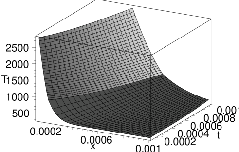
Figure 1: Exact solution of the problem (1)–(7) with parameters that are typical for aluminium: $\lambda_{1}=\lambda_{2}=240\,\frac{W}{K\cdot m},C_{1}=2,7\cdot 10^{6}\,\frac{J}{K\cdot m^{3}},C_{2}=2,74\cdot 10^{6}\,\frac{J}{K\cdot m^{3}},H_{v}=2,69\cdot 10^{10}\,\frac{J}{m^{3}},H_{m}=0,17\cdot 10^{10}\,\frac{J}{m^{3}},T_{0}=300\,K,T_{m}=933\,K$ and $T_{v}=2793\,K$ ; the energy flux was set $q=\frac{2,5\cdot 10^{8}}{\sqrt{t}}\,\frac{W}{m^{2}}.$

Example 2: $D_{1}(U)=\frac{a^{2}}{U^{2}},\ D_{2}(V)=\frac{b^{2}}{V^{2}}$.

According to case 2 of table 2, the general solutions of Eqs. (53) and (54) are

$$U=C_{1}\left(\frac{\sqrt{\pi}}{2}\,\textnormal{erf}(\tau)+C_{2}\right),\quad\omega=\frac{1}{a}\left(2\tau U+C_{1}e^{-{\tau}^{2}}\right),$$ (68)

$$V=C_{3}\left(\frac{\sqrt{\pi}}{2}\,\textnormal{erf}(\nu)+C_{4}\right),\quad\omega=\frac{1}{b}\left(2\nu V+C_{3}e^{-{\nu}^{2}}\right).$$ (69)

This is important to note that the second formula in (68) gives one-to-one correspondence between $\omega$ and $\tau$, because the differentiable function $\omega(\tau)$ is strictly monotonic:

$$\frac{d\omega}{d\tau}=\frac{1}{a}\left(2U+2\tau\frac{dU}{d\tau}+C_{1}(-2\tau)e^{-{\tau}^{2}}\right)=\frac{2}{a}\,U>0.$$ (70)

Hence, the function $\omega(\tau)$ is reversible and an inverse strictly monotonic function $\tau=\tau(\omega)$ exists for all $\omega>0$. Analogously, we prove the existence of an inverse strictly monotonic function $\nu=\nu(\omega)$ for the function $\omega(\nu)$ arising in the second formula of (69). With the monotonic differentiable functions $\tau(\omega)$ and $\nu(\omega)$, we transform the boundary conditions (55)–(59) with $D_{1}(U)=\frac{a^{2}}{U^{2}},D_{2}(V)=\frac{b^{2}}{V^{2}}$ to the form

$$\tau=\tau_{1}:\frac{dU}{d\tau}\left(\frac{d\omega}{d\tau}\right)^{-1}=\frac{\omega_{1}}{2}H_{v}-q_{0},$$ (71)

$$\tau=\tau_{1}:U=U_{1},$$ (72)

$$\tau=\tau_{2},\nu=\nu_{2}:\frac{dV}{d\nu}\left(\frac{d\omega}{d\nu}\right)^{-1}=\frac{dU}{d\tau}\left(\frac{d\omega}{d\tau}\right)^{-1}+\frac{\omega_{2}}{2}H_{m},$$ (73)

$$\tau=\tau_{2},\nu=\nu_{2}:U=U_{2},\ V=V_{2},$$ (74)

$$\nu=+\infty:V=V_{0}.$$ (75)

Substituting solutions (68) and (69) into the boundary conditions (72), (74) and (75), one finds the constants $C_{i}(i=1,...,4)$:

$$C_{1}=\frac{2}{\sqrt{\pi}}\frac{U_{2}-U_{1}}{\textnormal{erf}(\tau_{2})-\textnormal{erf}(\tau_{1})},\ C_{2}=\frac{\sqrt{\pi}}{2}\frac{U_{1}\,\textnormal{erf}(\tau_{2})-U_{2}\,\textnormal{erf}(\tau_{1})}{U_{2}-U_{1}},$$ (76)

$$C_{3}=\frac{2}{\sqrt{\pi}}\frac{V_{2}-V_{0}}{\textnormal{erf}(\nu_{2})-1},\ C_{4}=\frac{\sqrt{\pi}}{2}\frac{V_{0}\,\textnormal{erf}(\nu_{2})-V_{2}}{V_{2}-V_{0}}.$$ (77)

So, substituting formulae (76) and (77) into (68) and (69), respectively, we find the unknown functions in the explicit form

$$U=U_{1}+\frac{\textnormal{erf}(\tau)-\textnormal{erf}(\tau_{1})}{\textnormal{erf}(\tau_{2})-\textnormal{erf}(\tau_{1})}\,(U_{2}-U_{1}),\ \ \omega=\frac{2}{a}\left(\tau U+\frac{1}{\sqrt{\pi}}\frac{U_{2}-U_{1}}{\textnormal{erf}(\tau_{2})-\textnormal{erf}(\tau_{1})}\,e^{-\tau^{2}}\right),$$ (78)

$$V=V_{2}+\frac{\textnormal{erf}(\nu)-\textnormal{erf}(\nu_{2})}{\textnormal{erf}(\nu_{2})-1}\,(V_{2}-V_{0}),\ \ \omega=\frac{2}{b}\left(\nu V+\frac{1}{\sqrt{\pi}}\frac{V_{2}-V_{0}}{\textnormal{erf}(\nu_{2})-1}\,e^{-\nu^{2}}\right),$$ (79)

where $\tau_{1},\tau_{2},\nu_{2}$ are to-be-determined parameters. To find these positive parameters, one needs to substitute the functions $U$ and $V$ into (71) and (73), respectively. Moreover, the condition (see formulae (58))

$$\omega(\tau_{2})=\omega(\nu_{2})=\omega_{2}$$ (80)

should be taken into account. Finally, we arrive at the transcendent equation system

$$\frac{U_{2}-U_{1}}{\sqrt{\pi}}\left(\frac{a^{2}}{U_{1}}-H_{v}\right)\frac{e^{-{\tau}_{1}^{2}}}{\textnormal{erf}(\tau_{2})-\textnormal{erf}(\tau_{1})}=U_{1}H_{v}\tau_{1}-aq_{0},$$

$$\frac{ab}{\sqrt{\pi}}\frac{V_{2}-V_{0}}{V_{2}}\frac{e^{-{\nu}_{2}^{2}}}{\textnormal{erf}(\nu_{2})-1}=\frac{U_{2}-U_{1}}{\sqrt{\pi}}\left(\frac{a^{2}}{U_{2}}+H_{m}\right)\frac{e^{-\tau_{2}^{2}}}{\textnormal{erf}(\tau_{2})-\textnormal{erf}(\tau_{1})}+U_{2}H_{m}\tau_{2},$$ (81)

$$\frac{1}{a}\left(\tau_{2}U_{2}+\frac{1}{\sqrt{\pi}}\frac{U_{2}-U_{1}}{\textnormal{erf}(\tau_{2})-\textnormal{erf}(\tau_{1})}\,e^{-{\tau}_{2}^{2}}\right)=\frac{1}{b}\left(\nu_{2}V_{2}+\frac{1}{\sqrt{\pi}}\frac{V_{2}-V_{0}}{\textnormal{erf}(\nu_{2})-1}\,e^{-{\nu}_{2}^{2}}\right)$$

for finding the parameters $\tau_{1},\tau_{2}$ and $\nu_{2}.$

Thus, BVP (53)–(59) with $D_{1}(U)=\frac{a^{2}}{U^{2}},D_{2}(V)=\frac{b^{2}}{V^{2}}$ has the exact solution (78), (79) and

$$\omega_{1}=\frac{2}{a}\left(\tau_{1}U_{1}+\frac{1}{\sqrt{\pi}}\frac{U_{2}-U_{1}}{\textnormal{erf}(\tau_{2})-\textnormal{erf}(\tau_{1})}\,e^{-{\tau}_{1}^{2}}\right),$$ (82)

$$\omega_{2}=\frac{2}{a}\left(\tau_{2}U_{2}+\frac{1}{\sqrt{\pi}}\frac{U_{2}-U_{1}}{\textnormal{erf}(\tau_{2})-\textnormal{erf}(\tau_{1})}\,e^{-{\tau}_{2}^{2}}\right),$$ (83)

where the parameters $\tau_{1},\tau_{2}$ and $\nu_{2}$ are found from system (81).

Example 3: $D_{1}(U)=a^{2},D_{2}(V)=b^{2}e^{V}$, i.e., we consider the case when the basic equations (53) and (54) are essentially different.

According to cases 1 and 3 of table 2, the general solutions of Eqs. (53) and (54) are given by the formulae

$$U=C_{2}+C_{1}\frac{\sqrt{\pi}}{a}\,\textnormal{erf}\left(\frac{a\omega}{2}\right),$$ (84)

$$V=C_{4}+\int\limits_{c}^{\nu}\frac{d\nu}{g(\nu)},\ \omega=\nu e^{-\frac{V}{2}},\ C_{3}=\ln(2g-\nu)-\frac{\nu}{2g-\nu}-\frac{b^{2}}{4}{\nu}^{2},$$ (85)

where $c$ is an arbitrary constant.

In a quite similar way as was done in Example 2, one shows that the function $\omega(\nu)$ is reversible and an inverse strictly monotone function $\nu=\nu(\omega)$ exists for all $\omega>0$. So, using the monotonic differentiable function $\nu(\omega)$, we transform the boundary conditions (55)–(59) with $D_{1}(U)=a^{2},D_{2}(V)=b^{2}e^{V}$ to the form

$$\omega=\omega_{1}:U_{\omega}=\frac{\omega_{1}}{2}H_{v}-q_{0},$$ (86)

$$\omega=\omega_{1}:U=U_{1},$$ (87)

$$\nu=\nu_{2}:\frac{dV}{d\nu}\left(\frac{d\omega}{d\nu}\right)^{-1}=U_{\omega}+\frac{\omega_{2}}{2}H_{m},$$ (88)

$$\nu=\nu_{2}:U=U_{2},\ V=V_{2},$$ (89)

$$\nu=+\infty:V=V_{0},$$ (90)

where $\omega_{2}=\nu_{2}e^{-\frac{V_{2}}{2}}$.

The constants $C_{1},C_{2}$ and $C_{4}$ are defined by substitution (84) and (85) into the boundary conditions (87) and (89). So, we obtain after the corresponding calculations

$$C_{1}=\frac{a}{\sqrt{\pi}}\frac{U_{2}-U_{1}}{\textnormal{erf}\left(\frac{a\omega_{2}}{2}\right)-\textnormal{erf}\left(\frac{a\omega_{1}}{2}\right)},$$

$$C_{2}=\frac{U_{1}\,\textnormal{erf}\left(\frac{a\omega_{2}}{2}\right)-U_{2}\,\textnormal{erf}\left(\frac{a\omega_{1}}{2}\right)}{\textnormal{erf}\left(\frac{a\omega_{2}}{2}\right)-\textnormal{erf}\left(\frac{a\omega_{1}}{2}\right)},$$ (91)

$$C_{4}=V_{2}-\int\limits_{c}^{\nu_{2}}\frac{d\nu}{g(\nu)}.$$

The constant $C_{3}$ can be found using the third equation of (85) with $\nu=\nu_{2}$:

$$C_{3}=\ln(2g(\nu_{2})-\nu_{2})-\frac{\nu_{2}}{2g(\nu_{2})-\nu_{2}}-\frac{b^{2}}{4}\nu_{2}^{2}.$$ (92)

Substituting (91) into (84) and (85), we obtain

$$U=\frac{U_{1}\,\textnormal{erf}\left(\frac{a\omega_{2}}{2}\right)-U_{2}\,\textnormal{erf}\left(\frac{a\omega_{1}}{2}\right)+(U_{2}-U_{1})\,\textnormal{erf}\left(\frac{a\omega}{2}\right)}{\textnormal{erf}\left(\frac{a\omega_{2}}{2}\right)-\textnormal{erf}\left(\frac{a\omega_{1}}{2}\right)},$$ (93)

$$V=V_{2}+\int\limits_{\nu_{2}}^{\nu}\frac{d\nu}{g(\nu)},\ \ \omega=\nu e^{-\frac{V}{2}}.$$ (94)

Finally, substituting (93), (94) and (92) into the boundary conditions (86), (88) and (90) and making the corresponding simplification, we arrive at the transcendent equation system

$$\frac{a}{\sqrt{\pi}}\frac{U_{2}-U_{1}}{\textnormal{erf}\left(\frac{a\omega_{2}}{2}\right)-\textnormal{erf}\left(\frac{a\omega_{1}}{2}\right)}\,e^{-\frac{a^{2}\omega_{1}^{2}}{4}}=\frac{\omega_{1}}{2}H_{v}-q_{0},$$

$$V_{0}=V_{2}+\int\limits_{\nu_{2}}^{\infty}\frac{d\nu}{g(\nu)},$$

$$\ln(2g(\nu)-\nu)-\frac{\nu}{2g(\nu)-\nu}-\frac{b^{2}}{4}\nu^{2}=\ln(2g_{2}-\nu_{2})-\frac{\nu_{2}}{2g_{2}-\nu_{2}}-\frac{b^{2}}{4}{\nu_{2}}^{2},$$

where $g_{2}\equiv g(\nu_{2})=\frac{\nu_{2}}{2}+e^{\frac{V_{2}}{2}}\left(\frac{\omega_{2}}{2}H_{m}+\left(\frac{\omega_{1}}{2}H_{v}-q_{0}\right)\,e^{\frac{a^{2}}{4}(\omega_{1}^{2}-\omega_{2}^{2})}\right)^{-1}$.

4 Conclusions

In this paper, the (1+1)–dimensional nonlinear boundary value problem (9)–(15), modeling the process of melting and evaporation of metals, is studied by means of the classical Lie symmetry method. Theorem 2 that gives all possible Lie operators, which allow us to reduce the problem to the BVP for the ODE system, was proved. The forms of heat conductivity coefficients are established when the given problem can be analytically solved in an explicit form and the relevant exact solutions are constructed (see the formulae in examples 1–3).

We found that the case of a free boundary, which moves proportionally to $\sqrt{t}$, was earlier established for the classical Stefan problem with one moving boundary (solidification process) [14, 15]. In the particular case, one notes that formulae (64)–(67) with $\omega_{1}=0$ produce the corresponding solution obtained in [14] for the Stefan problem with one moving boundary. Similarly, formulae (78), (79) and (82) are generalizations of those from [15](see theorem 6) to the case of BVP with two moving boundaries. It should be noted that the authors of [14, 15] did not use any Lie symmetries but an assumption that $q(t)=\frac{q_{0}}{\sqrt{t}}$. In paper [16], a one-phase Stefan problem based on the linear heat equation was analytically solved using the above-mentioned assumption on the free boundary describing the movement of the shoreline. In [4], exact solutions are presented for several Stefan problems with different types of boundaries but with the linear basic equations.

To the best of our knowledge, there are only a few papers devoted to constructions of exact solutions of nonlinear boundary value problems of the Stefan type by means of the Lie symmetry method. Probably, paper [17] can be quoted as the first in this direction. Nevertheless, a Stefan type problem seems to be a more complicated object than the standard BVP with the fixed boundaries; one can note that the Lie symmetry method should be more applicable just for solving problems with moving boundaries. In fact, the structure of such boundaries may depend on invariant variable(s) and this gives a possibility of reducing the given BVP to one of lower dimensionality. The work is in progress to construct exact solutions of a a multidimensional BVP using this approach.

References

• [1] Ready J F 1971 Effects of High-power Laser Radiation (New York: Academic Press)
• [2] Rubinstein L I 1971 The Stefan problem (American Mathematical Society: Providence)
• [3] Crank J 1984 Free and moving boundary problems (Clarendon Press: Oxford)
• [4] Alexiades V and Solomon A 1993 Mathematical modeling of melting and freezing processes (Washington: Hemisphere publishing corporation)
• [5] Cherniha R M and Odnorozhenko I G 1990 Exact solutions of a nonlinear boundary value problem of melting and evaporation of metals under the action of high energy flux Dopovidi Akad. Nauk Ukrainy (Reports of Acad. Sci. of Ukraine), ser.A 12 44–47 (in Ukrainian, Summary in English)
• [6] Cherniga R M and Odnorozhenko I G 1991 Studies of the processes of melting and evaporation of metals under the action of laser radiation pulses Promyshlennaya Teplotekhnika (Industrial Heat Technic) 13 51–59 (in Russian, Summary in English)
• [7] Cherniha R M and Cherniha N D 1993 Exact solutions of a class of nonlinear boundary value problems with moving boundaries J. Phys. A.: Math. Gen. 26 L935–L940
• [8] Dulnyov G N and Yaryshev N A 1967 Estimation of process of heat-mass transfer by interaction of the energy flux with a substance Teplofizika vysokikh temperatur (Heatphysics of High Temperature) 5 322–328 (in Russian)
• [9] Ovsiannikov L V 1980 The Group Analysis of Differential Equations (New York: Academic Press)
• [10] Olver P 1986 Applications of Lie Groups to Differential Equations (Berlin: Springer)
• [11] Bluman G W and Kumei S 1989 Symmetries and Differential Equations (Berlin: Springer)
• [12] Fushchych W I, Serov M I and Amerov T K 1993 Nonlocal ansatze and solutions of nonlinear system of heat equatins Ukrainian Math. J. 45 293–302
• [13] Polyanin A D and Zaitsev V F 2003 Handbook of exact solutions for ordinary differential equations (Boca Raton, FL: CRC Press Company)
• [14] Tarzia D A 1981 An inequality for the coefficient $\sigma$ of the free boundary $s(t)=2\sigma\sqrt{t}$ of the Neumann solution for the two-phase Stefan problem Quart. Appl. Math. 39 491–497
• [15] Briozzo A C and Tarzia D A 2002 An explicit solution for an instantaneous two-phase Stefan problem with nonlinear thermal coefficients IMA Journal of Applied Mathematics 67 249–261
• [16] Voller V R, Swenson J B and Paola C 2004 An analytical solution for a Stefan problem with variable latent heat Int. J. Heat Mass Transfer 47 5387–5390
• [17] Bluman G 1974 Application of the general similarity solution of the heat equation to boundary-value problems Quart. Appl. Math. 31 403–415