Reaction Spreading on Graphs

Abstract

We study reaction-diffusion processes on graphs through an extension of the standard reaction-diffusion equation starting from first principles. We focus on reaction spreading, i.e. on the time evolution of the reaction product, $M(t)$. At variance with pure diffusive processes, characterized by the spectral dimension, $d_{s}$, for reaction spreading the important quantity is found to be the connectivity dimension, $d_{l}$. Numerical data, in agreement with analytical estimates based on the features of $n$ independent random walkers on the graph, show that $M(t)\sim t^{d_{l}}$. In the case of Erdös-Renyi random graphs, the reaction-product is characterized by an exponential growth $M(t)\sim e^{\alpha t}$ with $\alpha$ proportional to $\ln\langle k\rangle$, where $\langle k\rangle$ is the average degree of the graph.

A huge variety of different problems in chemistry, biology and physics deal with reactive species in non trivial substrates Murray . Seminal works on reaction and diffusion dynamics date back to the Fisher-Kolmogorov-Petrovskii-Piskunov (FKPP) model FKPP

$$\partial_{t}\theta=D\Delta\theta+f(\theta)\,,$$ (1)

where $D$ is the molecular diffusivity, $f(\theta)$ describes the reaction process and the scalar field $\theta$ represents the fractional concentration of the reaction products. Afterward, reaction-transport dynamics attracted a considerable interest for their relevance in a large number of chemical, biological and physical systems Murray .
Complex networks are a recent branch of graph theory becoming very important for different disciplines ranging from physics to social science, from biology to computer science Barabasi1999 . Although there exist an impressive amount of works on the study of both complex networks and reaction-transport processes, as far as we know, a general attempt to extend Eq. (1) on graphs and complex networks is still lacking.

There are two main approaches to study reaction dynamics on graphs. One concerns agent based models (Lagrangian description) in which random walkers move on the graph and interact, with a given reaction rule, when they occupy the same site at the same instant Kopelman1984 . A different approach is based on a mesoscopic description of the reaction dynamics (1) in which diffusion is modified introducing a proper transport term taking into account the feature of the media in which the dynamic takes place Mendez2010 . A particular approach in the mesoscopic description of the dynamics (used, e.g., in the recent field of epidemic spreading Vespignani2001 ), is to use a mean-field approximation in which a renormalized reaction term takes into account the network characteristics.

The goal of this letter is to study the reaction spreading on graphs extending model (1). In the presence of more general transport processes, the diffusion term $D\Delta\theta$ in Eq. (1), can be replaced by a suitable linear operator $\hat{L}$. A general evolution equation for $\theta$ is:

$$\partial_{t}\theta=\hat{L}\theta+\frac{1}{\tau}f(\theta)\,\,.$$ (2)

where we write explicitly the typical time scale, $\tau$, of the reaction process. An important class of processes of this type is the advection-reaction-diffusion (ARD), where $\hat{L}=-\mathbf{u}\cdot\mathbf{\nabla}+D\Delta$. Another interesting case is ruled by the effective diffusion operator $\hat{L}=\frac{1}{r^{d_{\tiny\mbox{f}}-1}}\frac{\partial}{\partial r}\left(k(r)r^{d_{\tiny\mbox{f}}-1}\frac{\partial}{\partial r}\right)$ Procaccia1985 suitable to study reaction dynamics on fractals Mendez2010 .

Equation (2) is constituted by two terms: the transport term, $\hat{L}\theta$, and the non-linear local reaction, $f(\theta)/\tau$. In the limit case without reaction, the link between the solution $\theta({\bf x},t)$ and a suitable stochastic process is quite clear: for instance, if $f(\theta)=0$ and $\hat{L}=-\mathbf{u}\cdot\mathbf{\nabla}+D\Delta$, Eq. (2) is nothing but the Fokker-Plank equation associated to the Langevin equation ${{\mathrm{d}}{\bf x}/{\mathrm{d}}t}={\bf u}+\sqrt{2D}{\mbox{\boldmath{$\eta$}}}.$ In general, even in the presence of reactive terms and for general $\hat{L}$, it is possible to write $\theta({\bf x},t)$ in terms of trajectories using the Freidlin formula Freidlin :

$$\theta(\mathbf{x},t)=\left\langle{\theta(\mathbf{x},0)\exp{\left(\frac{1}{\tau}\int_{0}^{t}\frac{f(\theta(\mathbf{x}(s;t),s))}{\theta(\mathbf{x}(s;t),s)}ds\right)}}\right\rangle$$ (3)

where the average is performed over all the trajectories ${\bf x}(s;t)$ starting in ${\bf x}(0)$ and ending in ${\bf x}(t;t)={\bf x}$. The possibility to write the generalization of (3) for a generic diffusive process has been discussed in acvv01 . Following this approach we can determine the dynamical equation of reaction diffusion on graphs.

As a diffusion process, we considered diffusion on an undirected, unweighted and connected graph $G=(V,E)$, where $V$ is the set of vertices of the graph (we consider a finite number, $N$, of vertices) and $E$ is the set of edges connecting the vertices. The graph can be represented by its adjacency matrix $A_{ij}$ given by bollobas1998 :

$$A_{ij}=\left\{\begin{array}[]{cl}1&{\rm if}\ (i,j)\in E\cr 0&{\rm if}\ (i,j)\not\in E\cr\end{array}\right.$$ (4)

The discrete Laplacian of the graph $\Delta_{ij}$ bollobas1998 ; bc05 is defined by: $\Delta_{ij}=A_{ij}-k_{i}\delta_{ij}$ where $k_{i}=\sum_{j}A_{ij}$, the number of nearest neighbors of $i$, is the degree of vertex $i$. Once the rate of the jump process, $w$, is introduced, the diffusion term can be written as

$$\frac{d\theta_{i}}{dt}=w\sum_{j}\Delta_{ij}\theta_{j}\,,$$ (5)

where $\theta_{i}$ is the concentration at vertex $i$. Our goal is to add to this equation a reaction term:

$$\frac{d\theta_{i}}{dt}=w\sum_{j}\Delta_{ij}\theta_{j}+\frac{1}{\tau}f(\theta_{i})\,.$$ (6)

The discrete-time version of the diffusion equation (5) is nothing but the random walk process described by the master equation

$$\theta_{n}(t+\Delta t)=\sum_{j}P_{j\to n}^{(\Delta t)}\theta_{j}(t)~{},$$ (7)

where jumps occur at time $\Delta t,2\Delta t,\ldots,$ and the probability for a walker being at vertex $i$ to jump to the vertex $j$ are given in terms of the adjacency matrix

$$\begin{array}[]{lcr}P_{i\to j}^{(\Delta t)}=wA_{ij}\Delta t&\text{if}&i\neq j\\ P_{i\to i}^{(\Delta t)}=1-k_{i}w\Delta t&\text{if}&i=j\end{array}$$ (8)

The discrete-time version of the reaction term can be defined as a non zero function only at discrete time when $\delta$-form impulses occur:

$$f(\theta,t)=\sum_{n=-\infty}^{\infty}g(\theta)\delta(t-n\Delta t)\,\Delta t\,\,,$$ (9)

where $g(\theta)$ is a suitable function. Such a choice for $f(\theta)$ allows us for a rigorous treatment of the discretization of the reaction term. With the above assumption, for Eq. (6) we have

$$\theta_{n}(t+\Delta t)=G_{\Delta t}\left(\sum_{j}P^{(\Delta t)}_{j\to n}\theta_{j}(t)\right)\,,$$ (10)

where $G_{\Delta t}(\theta)=\theta+g(\theta)\Delta t$ is the assigned reaction map. It is worth noting that Eq. (10) can be seen as a numerical method when the integration of (6) is performed in two steps: diffusion and then reaction acvv01 . The shape of the reaction map $G_{\Delta t}(\theta)$ depends on the underlying chemical model. For auto-catalytic pulled reactions (the FKPP class, where, e.g., $g(\theta)=\theta(1-\theta)/\tau$), characterized by an unstable fixed point in $\theta=0$ and a stable one in $\theta=1$ (the scalar field $\theta$ represents the fractional concentration of the reaction products; $\theta=1$ indicates the inert material, $\theta=0$ the fresh one, and $0<\theta<1$ means that fresh materials coexist with products) one can use $G_{\Delta t}(\theta)=\theta+\theta(1-\theta)\Delta t/\tau$. In the following we shall consider this type of reaction.

The most important topological features of a graph can be related to the spectral dimension, $d_{s}$, and the connectivity dimension, $d_{l}$, (also called chemical dimension). The former is related to diffusion processes on graphs and can be defined in terms of the return probability $P_{ii}$ at site $i$ for a random walker by $d_{s}=\lim_{t\rightarrow\infty}-2\frac{\ln P_{ii}(t)}{\ln t}$, or equivalently in terms of the density of eigenvalues of the Laplacian operator bc05 . The connectivity dimension measures the average number of vertices connected to a vertex in at most $l$ link, as $\#(l)\sim l^{d_{l}}$. For graphs embedded in an Euclidean space also the fractal dimension $d_{\tiny\mbox{f}}$ ccv should be considered, describing the scaling of the number of vertices in a sphere of radius $r$ in the Euclidean space, as $\#(r)\sim r^{d_{\tiny\mbox{f}}}$. The connectivity and fractal dimension can be different and they are related via the mapping between the two distances $r$ and $l$ Havlin1984 .

As a typical example of undirected, unweighted and connected graph, we show in Fig. 1 the reaction spreading in the T-graph Hav_84 .

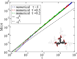
Figure 1: The percentage of quantity of product times $\tau$, $M(t)\tau$ vs $t$. Numerical results for Eq. (6) with $w=0.5$ are compared to prediction $t^{d_{l}}$. For this graph $d_{l}=\ln 3/\ln 2\simeq 1.585$, $d_{l}=2\ln 3/\ln 5\simeq 1.365$. Inset: Spreading on a T-fractal.

The field $\theta$ is initialized to zero in each vertex except the central one in which $\theta_{i}(0)=1$. Using Eq. (6) we study the time evolution of the system. An interesting observable to characterize the spreading of the reaction is the percentage of the total quantity of the reaction product, i.e., $M(t)=\frac{1}{N}\sum_{i\in V}\theta_{i}(t)$ where $N$ is the total number of vertices. As clearly shown in Fig. 1, $M(t)$ grows as a power law that can be interpreted as follows. Starting from a single vertex with $\theta_{i}(0)=1$, after $t$ step the number of vertices reached by the field is $\#(t)\sim t^{d_{l}}$. Therefore, in the limit of very fast reaction, when each vertex reached by the field is immediately burnt (i.e, $\theta_{j}\to 1$), we can expect:

$$M(t)\sim t^{d_{l}}.$$ (11)

Fig. 1 confirms that the connectivity dimension is the relevant quantity for the reaction spreading on graph. This behavior can be also understood thinking of the asymptotic behavior of the reaction process as determined by the spreading of the front in the topological metric of the graph. In this case the characteristic time of reaction, $\tau$, appears only in the prefactor of the exponential.

Moreover, a theoretical argument further confirms the importance of $d_{l}$. The analysis is based on an analogy between reaction spreading and short time regime of the number of distinct sites visited by $n$ independent random walkers after $t$ steps on a graph, $S_{n}(t)$ weiss . This quantity can be computed as $S_{n}(t)=\sum_{j=0}^{N}1-C_{0j}(t)^{n}$, where $C_{0j}(t)$ is the probability that a walker starting from site $0$ has not visited site $j$ at time $t$, the sum is over all the $N$ sites of the graph dropping the dependence on the starting site $0$. When the number of walkers is large ($n\to\infty$), $C_{0j}(t)^{n}$ tends to zero if site $j$ has a non zero probability of being reached in $t$ steps. In this limit, $S_{n}(t)$ represents all the sites which have nonzero probability of being visited by step t and, as $t$ is equal to the connectivity distance, $S_{n}(t)\sim t^{d_{l}}.$ This is precisely the regime observed in the reaction spreading (see Eq. (11) and Fig. 1). An estimate of the validity of the short time regime is given in terms of the smallest non zero occupation probability on the graph at time $t$, $P_{m}=\langle k\rangle^{-t}$, being $\langle k\rangle$ the average degree of the graph, i.e., the mean number of link for each vertex. As the short time regime is supposed to hold as long as $nP_{m}\gg 1$, one obtains that the reaction spreading regime is observed up to times $\bar{t}\sim\ln n$. On the other hand, the asymptotic regime is dominated by the number of distinct visited sites by a walker, that is $S_{n}(t)\sim t^{d_{s}/2}$ in graphs with compact exploration $d_{s}<2$, or simply by $t$ on graphs with $d_{s}>2$ weiss . In the case of very fast reaction regime, the front can be considered as equivalent to an infinite number of walkers, hence the asymptotic regime is never reached, leaving the dynamics to be governed by the sole $d_{l}$.

As for the spectral dimension, it is the relevant quantity when dealing with random-walk dynamics Kopelman1984 and in some reaction diffusion processes. For instance in bettolo Eq. (6) has been studied for coarsening processes where $f(\theta)$, at variance with our case, has a bistable structure. Moreover a further argument confirms the minor role of the spectral dimension in the case of reaction-diffusion dynamics using FKPP reaction terms. When dealing with standard diffusion ($\langle x^{2}(t)\rangle\sim t$) it is possible to show acvv01 that the spreading dynamics is the same displayed by the standard reaction/diffusion problem (1), i.e., $M(t)\sim t^{d}$ (where $d$ is the dimension of the space). On the other hand, the presence of anomalous diffusion ($\langle x^{2}(t)\rangle\sim t^{2\nu}$ with $\nu\neq 1/2$) does not implies that the spreading is anomalous: case exists acvv01 in which diffusion is anomalous but reaction spreading is standard.

The same behavior displayed in Figure 1 has been observed in several other self-similar graphs (e.g., Vicsek and Sierpinski carpet, not shown here), confirming the leading role of $d_{l}$. In the case of percolation clusters, the importance of the connectivity dimension, and the difference between connectivity dimension and fractal dimension was previously shown Havlin1984 .

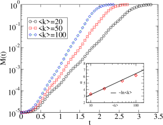
Figure 2: Reaction product $M(t)$ vs $t$ for Erdös-Renyi graphs. Three results for different average degree of connectivity are shown in the fast reaction regime ($\tau=0.1$). The reaction spreading follows an exponential behavior $M(t)\sim t^{\alpha}$, where $\alpha$ depends on $\langle k\rangle$ as shown in the inset.

Now we focus on the behavior of Eq. (6) for Erdös-Renyi (ER) random graphs bollobas1998 for which $d_{l}=\infty$. In the ER graphs two vertices are connected with probability $p$. We choose $p>\frac{\ln(N)}{N}$ so that the graph contains a global connected component. The average degree of the graph is $\langle k\rangle=p(N-1)\,.$ On ER graphs the number of points in a sphere of radius $l$ grows exponentially, $\#(t)\sim e^{c\,t}$, hence we expect a similar behavior for the spreading process:

$$M(t)\sim e^{\alpha t},$$ (12)

as shown in Fig 2. If $\langle k\rangle$ is large and the reaction is slow enough we have a two steps mechanism: first there is a rapid diffusion on the whole graph, then the reaction induces an increase of $\theta_{i}$. This leads to a simple mean field reaction dynamics, $\partial_{t}\rho(t)=\rho(t)(1-\rho(t))/\tau$, where $\rho$ is the average value of $\theta_{i}$ on the graph. In this case $\alpha=1/\tau$ as clearly observed in numerical simulations (not shown here).

In the much more interesting case of fast reaction, at each time step the number of sites invaded is proportional to the average degree of the graph, so that after $t$ steps we have:

$$M(t)\sim(C_{1}\langle k\rangle)^{t}=e^{C_{2}\ln\langle k\rangle t}\,,$$ (13)

leading to $\alpha\sim\ln\langle k\rangle$, see inset of Fig 2.

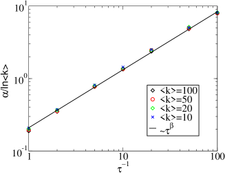
Figure 3: The scaling exponent $\alpha$ normalized with $\ln\langle k\rangle$, as a function of the inverse of reaction-time $\frac{1}{\tau}$. The straight line indicate $\tau^{\beta}$ with $\beta=-0.8$.

Furthermore, at variance with the case of graphs with finite $d_{l}$, at least in the case of fast reaction and FKPP reaction term, $\tau$ plays an important role since $C_{2}$ is a function of $\tau$. Fig. 3 shows the dependence of the exponential behavior of reaction spreading rescaled with $\ln\langle k\rangle$ as a function of $\tau$. We can fit the dependence of the curve on $\tau$ with $\alpha(k,\tau)\simeq C\tau^{\beta}\ln\langle k\rangle$, with $\beta\simeq-0.8$. This scaling can be related to a mean field-like equation of the type:

$$\partial_{t}\rho(t)=C\tau^{\beta}\ln(\langle k\rangle)\rho(t)(1-\rho(t))\,.$$ (14)

We have considered a general model for reaction-diffusion dynamics on graphs, allowing for a general and detailed treatment of the diffusive and reaction terms. We study only large systems in which the asymptotic scaling for the reaction spreading is well defined. On the other hand, although the spreading dynamics on small systems is certainly a very interesting issue, it deserves careful attention and it is beyond the scope of the present work. In fact, even in the absence of reaction (i.e., pure diffusion) in small systems the boundaries can induce rather complicated behaviours marchesoni .
On undirected and finite dimensional graphs, we found that a major role in the reaction spreading is played by the connectivity dimension, which rules the asymptotic of the reaction product as a function of time. On random graphs with infinite connectivity dimension, the reaction spreading shows an exponential behavior, whose scaling depends on the average degree of the graph. In this case, we obtain two mean-field like equations, one in the slow reaction limit and one in the fast reaction limit. In particular, in the fast reaction case, non-trivial dependence on both the average degree of the graph and the reaction characteristic time is shown. Our approach could be therefore suitable for a rigorous derivation of mean field like equations in more complex topologies.

References

- (1) J.D. Murray, Mathematical Biology, Springer-Verlag, Second Edition (1993); J. Xin, SIAM Review 42, 161 (2000); N. Peters, Turbulent combustion (Cambridge University Press, 2000).
- (2) A. N. Kolmogorov, I. G. Petrovskii, and N. S. Piskunov, Moscow Univ. Bull. Math. 1, 1 (1937); R. A. Fischer, Ann. Eugenics 7, 355 (1937).
- (3) A. L. Barabási and R. Albert, Science 286, 509 (1999); R. Cohen, S. Havlin and D. ben-Avraham, Phys. Rev. Lett. 91, 247901 (2003).
- (4) R. Kopelman, P. W. Klymko, J. S. Newhouse and L. W. Anacker, Phys. Rev. B 29, 3747 (1984); A. Barrat, M. Barthelémy, and A. Vespignani, Dynamical Processes on Complex Networks (Cambridge University Press, New York, 2008); E. Agliari, R.Burioni, D.Cassi, F.M. Neri, Theor. Chem. Acc. E 118, 855 (2007); E. Agliari, R.Burioni, D.Cassi, F.M. Neri, Diff. Fund.7 , 1.1 (2007).
- (5) V. Mendez, D. Campos and J. Fort, Phys. Rev. E 69, 016613 (2004). D. Campos, V. Mendez and J. Fort, Phys. Rev. E 69, 031115 (2004). V. Mendez, S. Fedotov, and W. Horsthemke, Reaction-Transport Systems: Mesoscopic Foundation, Fronts, and Spatial Instabilities (Springer-Verlag, Berlin, 2010)
- (6) R. Pastor-Satorras and A. Vespignani, Phys. Rev. Lett. 86, 3200 (2001).
- (7) B. O’Shaughnessy, I. Procaccia, Phys. Rev. Lett. 54(5), 455 (1985); L.P. Richardson, Proc. R. Soc. London A 110, 709 (1926).
- (8) M. Freidlin, Functional integration and partial differential equations (Princeton University Press, 1985).
- (9) M. Abel, A. Celani, D.Vergni and A. Vulpiani, Phys. Rev. E 64, 046307 (2001); R. Mancinelli, D. Vergni and A. Vulpiani, Physica D 185, 175 (2003).
- (10) B. Bollobás, Modern Graph theory (Springer-Verlag New York, 1998).
- (11) R. Burioni and D. Cassi, J. Phys. A. 38, R45 (2005).
- (12) M. Cencini, F. Cecconi and A. Vulpiani, Chaos (World Scientific, 2010).
- (13) S. Havlin and R. Nossal, J. Phys. A: Math. Gen. 17, L427 (1984); S. Havlin, D. ben-Avraham, Adv. Phys. 36, 695 (1987); H. E. Stanley and P. Trunfio, II Nuovo Cimento, 16 D, 1039 (1994); P. Meakin and H. E. Stanley, J. Phys. A: Math. Gen. 17, L173 (1984).
- (14) S. Havlin and H. Weissman, J. Phys. A: Math. Gen. 19, L1021 (1984).
- (15) G.H. Weiss, Aspects and Applications of the Random Walk (North-Holland, Amsterdam, 1994).
- (16) Umberto Marini Bettolo Marconi and A. Petri, Phys. Rev. E 55, 1311 (1997).
- (17) P. S. Burada, P. Hänggi, F. Marchesoni, G. Schmid, and P. Talkner, ChemPhysChem 10, 45 (2009).