Resonant states of deformed nuclei in complex scaling method

Abstract

We develop a complex scaling method for describing the resonances of deformed nuclei and present a theoretical formalism for the bound and resonant states on the same footing. With ³¹Ne as an illustrated example, we have demonstrated the utility and applicability of the extended method and have calculated the energies and widths of low-lying neutron resonances in ³¹Ne. The bound and resonant levels in the deformed potential are in full agreement with those from the multichannel scattering approach. The width of the two lowest-lying resonant states shows a novel evolution with deformation and supports an explanation of the deformed halo for ³¹Ne.

I Introduction

The investigation of continuum and resonant states is an important subject in quantum physics. In recent years, there has been an increasing interest in the exploration of nuclear single particle states in the continuum. The construction of the radioactive ion beam facilities makes it possible to study exotic nuclei with unusual N/Z ratios. In these nuclei, the Fermi surface is usually close to the particle continuum, thus the contribution of the continuum and/or resonances is essential for exotic nuclear phenomena Dobaczewski96 ; Poeschl97 ; Meng06 ; Hamamoto10 ; Zhou10 .

Several techniques have been developed to study the resonant states in the continuum. One of them is the R-matrix theory in which resonance parameters (i.e. energy and width) can be reasonably determined from fitting the available experimental data Wigner47 . The extended R-matrix theory Hale87 and the K-matrix theory Humblet91 have been also developed. The conventional scattering theory is also an efficient tool for studying resonances. More precisely, the scattering phase shift method is adopted and the resonant state is determined from the pole of the S matrix Taylor72 . Computationally, it is desired to deduce the properties of unbound states from the eigenvalues and eigenfunctions of the Hamiltonian for bound states so that the methods developed for bound states can still be used. For this purpose, bound-state-type methods have been developed, including the real stabilization method (RSM) Hazi70 , the complex scaling method (CSM) Ho83 , and the analytic continuation in the coupling constant (ACCC) method Kukulin89 . These bound-state-like methods have gained a great development. For examples, many efforts have been made in order to calculate more efficiently resonance parameters with the RSM Taylor76 ; Mandelshtam94 ; Kruppa99 . Its extension to the relativistic framework has been presentes in Ref. Zhang08 , where the resonance parameters obtained are comparable with those from the relativistic ACCC calculations. Combined with the cluster model, the ACCC approach has been used to calculate the energies and widths of resonant states in some light nuclei Tanaka97 ; Tanaka99 . An attempt to extend the ACCC approach to the relativistic mean field (RMF) model was made in Ref. Yang01 . Further development of the formalism was presented in Ref. Zhang04 , where the wave functions of the resonant states were determined by the ACCC method. Based on the relativistic extension of the ACCC method, the structure of resonant levels was investigated and good pseudospin symmetry was disclosed in realistic nuclei Guo05 ; Guo06 . Although it involves the solution of a complex eigenvalue problem which causes some difficulties in practice, the CSM has been widely and successfully used to study resonances in atomic and molecular systems Ho83 ; Moiseyev98 and atomic nuclei Kruppa97 ; Arai06 ; Aoyama06 ; Myo12 . Its generalization to the relativistic problem was first outlined by Weder Weder74 . Recent progress includes the following: Alhaidari Alhaidari07 has presented a general and systematic development of an algebraic extension of the CSM to the relativistic problem by expanding the Dirac spinors in Laguerre functions , Bylicki et al. Bylicki08 have formulated a positive-energy-space-projected relativistic Hylleraas configuration-interaction method based on the complex coordinate rotation , and we have developed the CSM within the RMF framework in satisfactory agreements with the RSM, the scattering phase-shift method and the ACCC approach Guo10 .

All these studies are mainly for spherical nuclei. Recently, the resonances of deformed nuclei have attracted additional attention. The interplay between the deformation and the low-lying resonance is very interesting for the open shell nucleus close to the drip line. The recent experimental data on the Coulomb breakup of the nucleus ³¹Ne Nakamura09 have been well interpreted in terms of deformation with particle populating in the resonant levels Hamamoto10 . The deformed halos have been investigated systemically in Ref. Zhou10 , where the resonances in the continuum play an important role. Some techniques have been developed to investigate the resonances of a deformed system. In Refs. Ferreira97 ; Yoshida05 , the resonances as a function of deformation in an axially deformed Woods-Saxon potential and a quadrupole-deformed finite square-well potential without a spin-orbit component have been studied by solving the coupled-channel Schrödinger equation. In Refs. Cattapan00 ; Hagino04 , the ACCC method and RSM have been extended to investigate the resonances in axially deformed Woods-Saxon potentials. The single-particle resonant states in an axially deformed Gaussian potential without spin and tensor components have been investigated by the contour-deformation method in momentum space Hagen06 . Using the multichannel scattering approach, Hamamoto Hamamoto05 has studied how the single-particle energies change from bound to resonant levels when the depth of the potential is varied. This method has also been applied for the resonances of a Dirac particle in a deformed potential Li10 . Hamamoto Hamamoto12 has performed a systematic research on the resonances of deformed nuclei by the multichannel scattering approach, which includes the evolution of shell structure for exotic nuclei. However, as we know, CSM has not been used to investigate the resonances of deformed nuclei. Due to the great success of CSM in describing the resonances for a spherical system, in this paper, we extend CSM to a deformed system, and examine its applicability and efficiency for the resonances of deformed nuclei.

II Formalism

Our purpose is to extend the CSM to describe the resonances of deformed nuclei. This scheme has a certain advantage, i.e., the bound and resonant states can be treated on the same footing, because the complex scaled functions for the resonant states are square integrable just like those for the bound states Moiseyev98 . In the following, we start our scenario with the single-particle Hamiltonian give as

$$H=T+V\ ,$$ (1)

where $V$ is introduced with the axially symmetric quadruple-deformed potential consisting of the following three parts:

$$V_{\text{cent}}\left(r\right) = V_{0}f\left(r\right),$$

$$V_{\text{cou}}\left(\vec{r}\right) = -\beta_{2}V_{0}k\left(r\right)Y_{20}\left(\vartheta,\varphi\right),$$

$$V_{\text{so}}\left(r\right) = -\frac{1}{2}vV_{0}g(r)\left(\vec{s}\cdot\vec{l}\right).$$ (2)

Here $k\left(r\right)=r\frac{df\left(r\right)}{dr}$ and $g(r)=\frac{\Lambda^{2}}{r}\frac{df\left(r\right)}{dr}$. The parameter $\Lambda$ is the reduced Compton wavelength of nucleon $\hslash/M_{r}c$. Similar to Ref.Hamamoto05 , a Woods-Saxon type potential is employed for $f\left(r\right)=\frac{1}{1+\exp\left(\frac{r-R}{a}\right)}$. To explore the resonant states, the CSM is used. A relative coordinate $r$ in Hamiltonian $H$ and wave function $\psi$ is complex scaled as

$$U(\theta):r\rightarrow re^{i\theta}.$$ (3)

Then, the transformed Hamiltonian and wave function are defined as $H_{\theta}=U\left(\theta\right)HU\left(\theta\right)^{-1}$ and $\psi_{\theta}=U\left(\theta\right)\psi$, where $\psi_{\theta}$ is a square integrable function. The corresponding complex scaled equation is

$$H_{\theta}\psi_{\theta}=E_{\theta}\psi_{\theta}.$$ (4)

From ABC theoremAguilar71 , the following is known: (i) a bound-state eigenvalue of $H$ is also an eigenvalue of $H_{\theta};$ (ii) a resonance pole $E=E_{r}-i\Gamma/2$ of the Green operator of $H$ is an eigenvalue, $E_{\theta}=E_{r}-i\Gamma/2$ of $H_{\theta}$; and (iii) the continuous part of the spectrum is rotated around the origin of the $E-$ plane by an angle $2\theta$.

To solve the complex scaled equation (4), it is convenient to adopt the basis expansion method. For the axially symmetrically deformed system, the parity $\pi=(-1)^{N}=(-1)^{l}$ and the projection of the total angular momentum along the symmetry axis $\Omega$ are good quantum numbers; $\psi_{\theta}$ can be expanded as

$$\psi_{\theta}=\sum_{i}c_{i}\left(\theta\right)\phi_{i}\text{ },$$ (5)

where $\phi_{i}=R_{nl}(r)Y_{lm_{l}}(\vartheta,\varphi)\chi_{m_{s}}(\sigma_{z})$ and the sum $i$ runs over the quantum numbers $n,l,$and $m_{l}$ with $\Omega=m_{l}+m_{s}$. $R_{nl}(r)$ is the radial function of a spherical harmonic oscillator (HO) potential,

$$R_{nl}(r)=\frac{1}{b_{0}^{3/2}}\sqrt{\frac{2\left(n-1\right)!}{\Gamma\left(n+l+1/2\right)}}x^{l}L_{n-1}^{l+1/2}\left(x^{2}\right)e^{-x^{2}/2}\text{, }n=1,2,3,\text{ }....$$ (6)

$x=r/b_{0}$ is the radius measured in units of the oscillator length $b_{0}$. $Y_{lm_{l}}(\vartheta,\varphi)$ is the spherical harmonics. $\chi_{m_{s}}(\sigma_{z})$ represents the spin wave function. The upper limit of the radial quantum number $n$ is determined by the corresponding major shell quantum number $N=2\left(n-1\right)+l$. Inserting the ansatz (5) into the complex scaled equation (4) and using the orthogonality of wave functions $\phi_{i}$ one arrives at a symmetric matrix diagonalization problem,

$$\sum_{i}\left[T_{i^{\prime},i}+V_{i^{\prime},i}\right]c_{i}=E_{\theta}c_{i^{\prime}}\text{ },$$ (7)

where $T_{i^{\prime},i}$ and $V_{i^{\prime},i}$ are presented as

$$T_{i^{\prime},i} = e^{-i2\theta}\int\phi_{i^{\prime}}\left(-\frac{\hbar^{2}}{2M}\left(\frac{d^{2}}{dr^{2}}+\frac{2}{r}\frac{d}{dr}\right)+\frac{\vec{l}^{2}}{2Mr^{2}}\right)\phi_{i}d\vec{r}\text{ },$$ (8)

$$V_{i^{\prime},i} = \int\phi_{i^{\prime}}V\left(\vec{r}e^{i\theta}\right)\phi_{i}d\vec{r}\text{ }.$$ (9)

Putting $\phi_{i}$ into the above expressions, the matrix elements $T_{i^{\prime},i}$ are obtained as

$$T_{i^{\prime},i}=e^{-i2\theta}\frac{\hbar^{2}}{2Mb_{0}^{2}}\left[\sqrt{n\left(n+l+1/2\right)}\delta_{n^{\prime},n+1}+(2n+l-1/2)\delta_{n^{\prime},n}+\sqrt{\left(n-1\right)\left(n+l-1/2\right)}\delta_{n^{\prime},n-1}\right]\delta_{l^{\prime}l}\delta_{m_{l}^{\prime}m_{l}}\delta_{m_{s}^{\prime}m_{s}}$$ (10)

Similarly, the matrix elements $V_{i^{\prime},i}$ are obtained as

$$V_{i^{\prime},i}^{\text{cent}} = \left\langle\phi_{i^{\prime}}\right|V_{\text{cent}}(re^{i\theta})\left|\phi_{i}\right\rangle=V_{0}\left\langle n^{\prime}l^{\prime}\right|f(re^{i\theta})\left|nl\right\rangle\delta_{l^{\prime}l}\delta_{m_{l}^{\prime}m_{l}}\delta_{m_{s}^{\prime}m_{s}}\text{ },$$ (11)

$$V_{i^{\prime},i}^{\text{cou}} = \left\langle\phi_{i^{\prime}}\right|V_{\text{cou}}\left(\vec{r}e^{i\theta}\right)\left|\phi_{i}\right\rangle=-\beta_{2}V_{0}\left\langle n^{\prime}l^{\prime}\right|k\left(re^{i\theta}\right)\left|nl\right\rangle\left\langle l^{\prime}m_{l}^{\prime}\right|Y_{20}\left(\vartheta,\varphi\right)\left|lm_{l}\right\rangle\delta_{m_{s}^{\prime}m_{s}}\text{ },$$ (12)

$$V_{i^{\prime},i}^{\text{so}} = \left\langle\phi_{i^{\prime}}\right|V_{\text{so}}\left|\phi_{i}\right\rangle=-\frac{1}{2}vV_{0}\left\langle n^{\prime}l^{\prime}\right|g(re^{i\theta})\left|nl\right\rangle\left\langle l^{\prime}m_{l}^{\prime}m_{s}^{\prime}\right|\left(\vec{s}\cdot\vec{l}\right)\left|lm_{l}m_{s}\right\rangle\text{ }.$$ (13)

In these expressions, $\left\langle l^{\prime}m_{l}^{\prime}\right|Y_{20}\left(\vartheta,\varphi\right)\left|lm_{l}\right\rangle$ and $\left\langle l^{\prime}m_{l}^{\prime}m_{s}^{\prime}\right|\left(\vec{s}\cdot\vec{l}\right)\left|lm_{l}m_{s}\right\rangle$ can be calculated by the usual angular momentum formulas, and the radial parts of integration can be calculated with the Gauss quadrature approximation. With the matrix elements $T_{i^{\prime},i}$, $V_{i^{\prime},i}^{\text{cent}}$, $V_{i^{\prime},i}^{\text{cou}},$ and $V_{i^{\prime},i}^{\text{so}}$, the solutions of the complex scaling equation (4) can be obtained by diagonalizing the matrix $H_{\theta}$. The eigenvalues of $H_{\theta}$ representing bound states or resonant states do not change with $\theta$, while the eigenvalues representing the continuous spectrum rotate with $\theta$. The former are associated with resonance complex energies $E-i\Gamma/2$, where $E$ is the resonance position and $\Gamma$ is its width.

III Numerical details and Results

With the theoretical formalism, we explore the resonant states for the realistic physical system. In the numerical details, the complex-scaled Schrödinger equation is solved by expansion in the HO basis with $60$ oscillator shells. The oscillator frequency of the HO basis is fixed as $\hslash\omega_{0}=41A^{-1/3}$ MeV. For the comparison with the results from the multichannel scattering approach Hamamoto05 , ³¹Ne is taken as an example. The corresponding parameters are chosen to be same as those in Ref.Hamamoto10 , i.e., $a=0.67$ fm, $V_{0}=-39$ MeV, $v=32$, and the nuclear radius $R$ varying with the mass number $A$ of the system with $R=r_{0}A^{1/3},$ where $r_{0}=1.27$ fm is used. To achieve the information on the resonant states, we diagonalize $H_{\theta}$. The eigenvalues of $H_{\theta}$ for these states with the quantum numbers varying from $\Omega^{\pi}=\frac{1}{2}^{\pm}$ to $\Omega^{\pi}=\frac{9}{2}^{\pm}$ are plotted in Fig.1, where the rotation angle $\theta=18^{\circ}$ and the quadruple deformation $\beta_{2}=0.1$ are adopted. All the eigenvalues of $H_{\theta}$, which correspond to the bound, the resonant, and the continuum, are respectively labeled as open squares, red open circles, and open circles. The solid line marks the position of the continuum with the rotation angle $2\theta$. From Fig.1, one sees clearly that the eigenvalues of $H_{\theta}$ fall into three regions: the bound states populate on the negative energy axis, while the continuous spectrum of $H_{\theta}$ rotates clockwise with the angle $2\theta$, and resonances in the lower half of the complex energy plane located in the sector bound by the new rotated cut line and the positive energy axis get exposed and become isolated. In realistic calculations, because the finite basis is used, the continuous spectrum of $H_{\theta}$ consists of a string of points.

Next, we demonstrate how the resonant states become exposed by complex rotation. The eigenvalues of $H_{\theta}$ with $\theta=8^{\circ},12^{\circ},16^{\circ},$and $20^{\circ}$ are respectively displayed in Figs.2(a)-2(d), where the other parameters are the same as those in Fig.1. From Fig.2 one can see that, when $\theta=8^{\circ}$, the resonances still have not been completely separated from the continuum, and to identify the resonances in the continuum is still relatively difficult although several points are marked as the resonances in the complex energy plane. When the rotation angle is added to $\theta=12^{\circ}$, the resonant states are clearly isolated from the continuum and distinguishing the resonances from the continuum becomes easy. When the rotation angle is added to $\theta=16^{\circ}$, the resonant states are completely separated from the continuum, and clearly exposed in the complex energy plane. This is because the continuous spectrum of $H_{\theta}$ rotates clockwise with ${\theta}$, while the resonances are almost independent of the rotation angle $\theta$. From Figs.2(c) and 2(d), the rotation angle is incresed from $\theta=16^{\circ}$ to $\theta=20^{\circ}$, and the change of position of the resonant states in the complex energy plane is almost not observable. This indicates that the resonant states can be unambiguously determined at the same time as long as the rotation angle is chosen to be large enough, which is one of the advantages of CSM. In the present calculations, the exposure of the resonant states relies on the scale of the rotation angle, while their position in the complex energy plane remains almost unchanged with the variation of $\theta$; i.e., the energies and widths are nearly $\theta$ independent, which also reflects that the stability of the results with respect to the variation of $\theta$ is considerably satisfactory.

As we look forward to the resonances of the deformed nuclei states, it is interesting to observe the movement of the resonant states in the position with deformation in the complex energy plane, which is helpful to recognize intuitively the resonances of the deformed nuclei. In Fig.3, we show the eigenvalues of $H_{\theta}$ with deformation $\beta_{2}=0.0,-0.1,-0.2,$and $-0.3$. The other parameters are the same as those in Fig.1. When the system is spherically symmetrical ($\beta_{2}=0.0$), only three resonances are observed, which correspond respectively to the resonant states $1f_{7/2},1f_{5/2}$, and $1g_{9/2}$. When the spherical symmetry of the system is broken ($\beta_{2}\neq 0.0$), the 3 resonances are broken down into 12 resonances, which correspond respectively to the resonant states 1/2[330], 3/2[321], 5/2[312], 7/2[303], 1/2[310], 3/2[301], 5/2[303], 1/2[440], 3/2[431], 5/2[422], 7/2[413], and 9/2[404] (denoted with the asymptotic quantum numbers $\Omega[Nn_{z}\Lambda])$. The location of the 12 resonant states in the complex energy plane appears to be a significant movement when the deformation is changed. With the development of deformation towards the direction of larger deformation, the 12 resonant states in the position are more clearly separated. The similar movement of the position towards the prolate shapes has also been obtained, and not been displayed here.

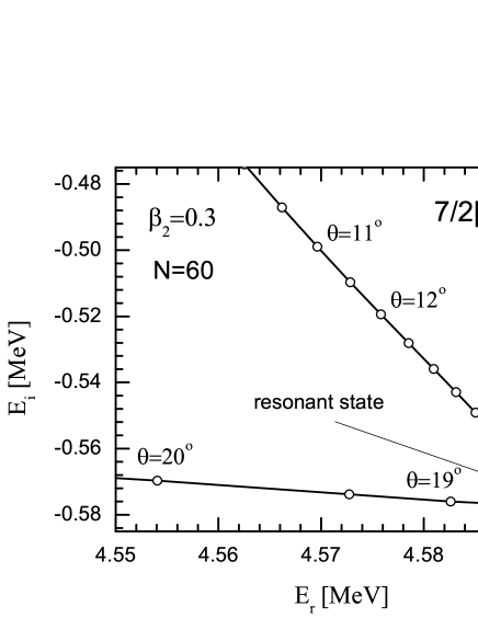
Fig 5: The same as Fig.4, but a close up of the $\theta$ trajectory in Fig.4 for $N=60$, where the arrow marks the position of the resonant state.

Although the resonances of several points of deformation are displayed in Fig.3, the resonance parameters of these points have not been fully determined for the resonant states exposed in Fig.1. In the following, we check how the results depend on $\theta$ in the present calculations in order to present the accurate values of the resonance parameters. According to the mathematical theorem the resonance energies should be independent of $\theta$ (for large enough $\theta$). However, in the present numerical approximation, resonance parameters are dependent slightly on $\theta$ due to basis expansion with finite shells, there will be no eigenvector that is completely independent of $\theta$. The resonance energies will move along trajectories in the complex energy plane as a function of $\theta$. The best estimate for a resonance energy is given by the parameter $\theta$ value for which the rate of change with respect to $\theta$ is minimal. To locate the minimal rate point, we perform repeated diagonalizations of the eigenvalue problem of $H_{\theta}$ with different $\theta$ values in every deformation concerned. The illustrated results are shown in Fig.4 for the resonant state 7/2[303] of the deformation point $\beta_{2}=0.3$, where $N$ represents the number of oscillator shells of the basis. From Fig.4 one sees clearly that, for different $N$, the dependence of the resonance parameters on $\theta$ shows a different trajectory, and the range of the trajectory becomes smaller with the increasing $N$ when $N\geqslant 50$. In every $\theta$-trajectory, there exists a point corresponding to the minimal rate of change of the resonance parameters with respect to $\theta$, which presents the optimal value of the resonance parameters. Despite the difference in the $\theta$ trajectory, the optimal value of the resonance parameters tends to the same result with the increasing $N$, especially when $N\geqslant 50$. Although the movement of the optimal value in the complex energy surface is observable, that is because we display these results in a small energy scale. Compared with the continuous spectra, the movement is negligible, especially when $N\geqslant 50$. Hence, the size of the basis being chosen as $N=60$ is good enough in the previous calculations. To more accurately determine the value of the resonance parameters, a close up of the $\theta$ trajectory is plotted in Fig.5 for $N=60$. In the vicinity of $\theta=17^{\circ}$, the resonance parameters are almost independent of $\theta$, i.e., $\frac{dE_{\theta}}{d\theta}\approx 0$, which presents the optimal value of the resonance parameters.

By using the $\theta$ trajectory, the resonance parameters of any deformation point can be determined for the resonant states exposed in Fig.1. In Fig.6, we show the evolution of the single-particle energy with the deformation $\beta_{2}$ for the bound and resonant states. In comparison with Ref.Hamamoto10 , consistent results are obtained for the bound levels and the low-lying resonant levels. In addition, several higher-lying resonant levels are also obtained in the present calculations. Especially, the width is obtained for all the resonant states. In Fig.7, we plot the width for the four lower-lying resonant states 1/2[330], 3/2[321], 5/2[312], and 7/2[303]. For the resonant state 7/2[303], the resonance energy and the width increase monotonously with the deformation varying from $\beta_{2}=-0.4$ to $0.6$. For the resonant state 5/2[312], the energy and the width display an almost horizontal change with the deformation. For the resonant states 1/2[330] and 3/2[321], with the deformation varying from $\beta_{2}=-0.4$ to $0.6$, the energy decreases monotonously, while the width shows a unusual trend. Close to $\beta_{2}=0.0$, the value of the width appears to be at a minimum, which implies the spherical shape is more stable for the two resonant states. After the minimum appears, the resonance width increases with the increasing of deformation, which means these nuclei states become even more unstable as their levels become lower. With a continued increase in deformation, the width appears to be at a maximum value. Therefore, it is relatively difficult for the halo to forming in the deformation interval from $\beta_{2}=0.0$ to the position of the width appearing at a maximum value for ³¹Ne. Thereafter, the resonance width decreases with the increase in deformation. When the deformation increases beyond $\beta_{2}=0.25$, the level 1/2[330] becomes weakly bound. In the vicinity of $\beta_{2}=0.3$, the levels 1/2[330] and 3/2[202] appear to be crossing. With a further increase in deformation, the energy gap between 1/2[330] and 3/2[202] gets larger and a maximum appears at $\beta_{2}=0.43$. Thus, in this deformation interval from $\beta_{2}=0.25$ to $\beta_{2}=0.43$, the 21th neutron can occupy the weakly bound level 1/2[330] or 3/2[202], and the halo can be formed there. The most likely position for forming a halo should be near $\beta_{2}=0.3$. This information indicates that ³¹Ne may be a halo nucleus with deformation $\beta_{2}\sim 0.3$.

IV Summary

In summary, the complex scaling method is extended to describe the resonances of deformed nuclei. A theoretical formalism is presented in which the bound and resonant states are treated on the same footing. ³¹Ne is chosen as an example; the utility and applicability of the extended method are demonstrated. It is found that the exposure of resonant states relies on the scale of the rotation angle, while their position in the complex energy plane remains almost unchanged with the variation of $\theta$, which reflects that the stability of the results with respect to the variation of $\theta$ is considerably satisfactory. The movement of the resonant states in the position with deformation is exhibited in complex energy plane, where it is seen that 3 degenerate resonances are separated into 12 resonances with the development of deformation towards the oblate or prolate shapes. The bound and resonant levels obtained for ³¹Ne are in agreement with those from the coupling-channel calculations, where the resonances are determined by a multichannel scattering approach. With the deformation evolution from the oblate to prolate shapes, the bound and resonant levels show a clear shell structure. Especially, the width of the two lowest-lying resonant states shows a novel evolution with deformation, and supports an explanation of the deformed halo for ³¹Ne.

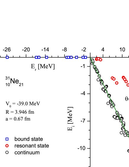
Fig 1: (Color online) The eigenvalues of the complex scaled Hamiltonian $H_{\theta}$ for the states $\Omega^{\pi}=\frac{1}{2}^{\pm},\frac{3}{2}^{\pm},\dots,\frac{9}{2}^{\pm}$ in the present calculations with the complex scaling parameter $\theta=18^{\circ}$ and the quadrupole deformation $\beta_{2}=0.1$. The calculations are performed by basis expansion with 60 HO shells. The bound states, the resonant states, and the continuum are respectively labeled as open squares, red open circles, and open circles. The solid line rotating with $2\theta$ marks the position of the continuous spectra.

Fig 2: (Color online) The resonant and continuous spectra varying with the complex rotation angle associated with the model. Except for the complex rotation angle, the other parameters are the same as those in Fig.1.

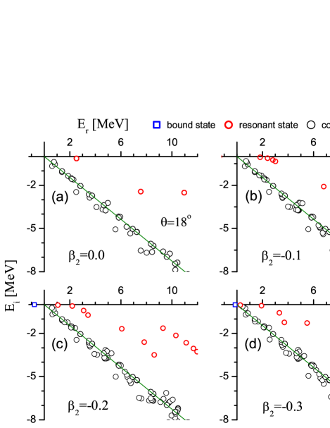
Fig 3: (Color online) The movement of the resonant states in the position with deformation in the complex energy plane, where the development of deformation is towards the direction of oblate shapes and the parameters adopted are the same as those in Fig.1 except for a different deformation in every configure.

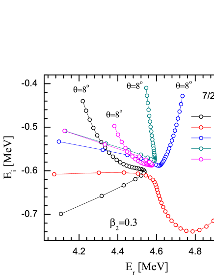
Fig 4: (Color online) The $\theta$ trajectories corresponding to the several different numbers of oscillator shells of the basis for the resonant state 7/2[303] of the deformation point $\beta_{2}=0.3$, where $N$ is the quantum number of the main shell of the oscillator basis, and $\theta$ varies from $8^{\circ}$ to $22^{\circ}$ by steps of $0.5^{\circ}$.

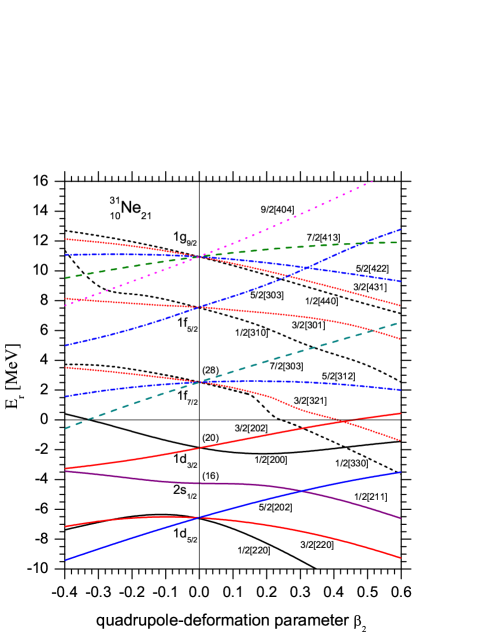
Fig 6: (Color online) Neutron single-particle levels in Woods-Saxon potentials as a function of the quadrupole deformation parameter $\beta_{2}$. The depth, the diffuseness, and the radius of the potential are -39 MeV, 0.67 fm, and 3.946 fm, respectively. Every level is labeled with the asymptotic quantum numbers $\Omega$[N$n_{z}\Lambda$].

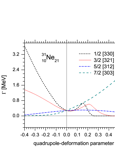
Fig 7: (Color online) The same as Fig.6, but for the width of the four resonant states 1/2[330], 3/2[321], 5/2[312], and 7/2[303].

- (1) J. Dobaczewski, W. Nazarewicz, T. R. Werner, J.-F. Berger, C. R. Chinn, and J. Dechargé, Phys. Rev. C 53, 2809 (1996).
- (2) W. Pöschl, D. Vretenar, G. A. Lalazissis, and P. Ring, Phys. Rev. Lett. 79, 3841 (1997).
- (3) J. Meng, H. Toki, S.-G. Zhou, S. Q. Zhang, W. H. Long, and L. S. Geng, Prog. Part. Nucl. Phys. 57, 470 (2006).
- (4) I. Hamamoto Phys. Rev. C 81, 021304(R) (2010).
- (5) S. G. Zhou, J. Meng, P. Ring, and E. G. Zhao, Phys. Rev. C 82, 011301(R) (2010).
- (6) E. Wigner and L. Eisenbud, Phys. Rev. 72, 29 (1947).
- (7) G. M. Hale, R. E. Brown, and N. Jarmie, Phys. Rev. Lett. 59, 763 (1987).
- (8) J. Humblet, B. W. Filippone, and S. E. Koonin, Phys. Rev. C 44, 2530 (1991).
- (9) J. R. Taylor, Scattering Theory: The Quantum Theory on Nonrelativistic Collisions, (John Wiley & Sons, New York, 1972).
- (10) A. U. Hazi and H. S. Taylor, Phys. Rev. A 1, 1109 (1970).
- (11) Y. K. Ho, Phys. Rep. 99, 1 (1983).
- (12) V. I. Kukulin, V. M. Krasnopl’sky, and J. Horácek, Theory of Resonances: Principles and Applications (Kluwer Academic, Dordrecht, 1989).
- (13) H. S. Taylor and A. U. Hazi, Phys. Rev. A 14, 2071 (1976).
- (14) V. A. Mandelshtam, H. S. Taylor, V. Ryaboy, and N. Moiseyev, Phys. Rev. A 50, 2764 (1994).
- (15) A. T. Kruppa and K. Arai, Phys. Rev. A 59, 3556 (1999).
- (16) L. Zhang, S. G. Zhou, J. Meng, and E. G. Zhao, Phys. Rev. C 77, 014312 (2008).
- (17) N. Tanaka, Y. Suzuki, and K. Varga, Phys. Rev. C 56, 562 (1997).
- (18) N. Tanaka, Y. Suzuki, K. Varga, and R. G. Lovas, Phys. Rev. C 59, 1391 (1999).
- (19) S. C. Yang, J. Meng, and S. G. Zhou, Chin. Phys. Lett. 18, 196 (2001).
- (20) S. S. Zhang, J. Meng, S. G. Zhou, and G. C. Hillhouse, Phys. Rev. C 70, 034308 (2004).
- (21) J.Y. Guo, R.D. Wang, and X.Z. Fang, Phys. Rev. C 72, 054319 (2005).
- (22) J.Y. Guo and X.Z. Fang, Phys. Rev. C 74, 024320 (2006).
- (23) N. Moiseyev, Phys. Rep. 302, 212 (1998).
- (24) A. T. Kruppa, P. -H. Heenen, H. Flocard, and R. J. Liotta, Phys. Rev. Lett. 79, 2217 (1997).
- (25) K. Arai, Phys. Rev. C 74, 064311 (2006).
- (26) S. Aoyama, T. Myo, K. Katō, and K. Ikeda, Prog. Theor. Phys. 116, 1 (2006).
- (27) T. Myo, Y. Kikuchi, and K. Kato, Phys. Rev. C 85, 034338 (2012), and references therein.
- (28) R. A. Weder, J. Math. Phys. 15, 20 (1974).
- (29) A. D. Alhaidari, Phys. Rev. A 75, 042707 (2007).
- (30) M. Bylicki, G. Pestka, and J. Karwowski, Phys. Rev. A 77, 044501 (2008).
- (31) J. Y. Guo, X. Z. Fang, P. Jiao, J. Wang, and B. M. Yao, Phys. Rev. C 82, 034318 (2010).
- (32) T. Nakamura et al., Phys. Rev. Lett. 103, 262501 (2009).
- (33) L. S. Ferreira, E. Maglione, and R. J. Liotta, Phys. Rev. Lett. 78, 1640 (1997).
- (34) K. Yoshida and K. Hagino, Phys. Rev. C 72, 064311 (2005).
- (35) G. Cattapan and E. Maglione, Phys. Rev. C 61, 067301(2000).
- (36) K. Hagino and N. Van Giai, Nucl. Phys. A 735, 55 (2004).
- (37) G. Hagen and J. S. Vaagen, Phys. Rev. C 73, 034321 (2006).
- (38) I. Hamamoto, Phys. Rev. C 72, 024301 (2005).
- (39) Z. P. Li, J. Meng, Y. Zhang, S. G. Zhou, and L. N. Savushkin, Phys. Rev. C 81, 034311 (2010).
- (40) I. Hamamoto, Phys. Rev. C 85, 064329 (2012).
- (41) J. Aguilar and J. M. Combes, Commun. Math. Phys. 22, 269 (1971); E. Balslev and J. M. Combes, ibid. 22, 280 (1971).