An Empirical Investigation of Scaling Behavior in the Atmospheric Turbulence for Understanding the Underlying Cascade Process

Abstract

We study the scaling behaviors in the wind velocity time series collected at the atmospheric surface layer and compare them with two commonly used cascade models, the truncated stable distribution and the log-normal model. Results show that although both models can describe the change of probability density functions from non-Gaussian to Gaussian like distributions with the increase of time scale, they can not fit the scaling behaviors observed in the probability of return and in the moments at the same time. This work provides some clues on the understanding of cascade process in the atmospheric turbulence.

1 Introduction

The probability density functions (PDFs) of the atmospheric turbulent velocity increments have been found to go from Gaussian like behavior at a time scale of few days to stretched exponential like behavior at a time scale of one hour [1]. This behavior is similar to that observed in fully developed homogeneous and isotropic turbulence, where it has long been recognized that the energy is transferred from large scales to smaller scales by some cascade process. Although the atmospheric turbulence is obviously non-homogenous and non-isotropic, its statistical similarity with homogeneous and isotropic turbulence suggests that there may be also some cascade process associated with the energy transfer between synoptic scales and smaller scales in the atmospheric turbulence.

To our knowledge, two models are commonly used to describe the PDFs of atmospheric turbulent velocity increments. One is the log-normal model which was proposed to account for the intermittency in the local homogeneous and isotropic turbulence [2]. The other is the truncated stable distribution (sometimes called truncated Lévy distribution), which was originally proposed to resolve the paradox between infinite variance of stable distribution and finite variance of real economic systems [3, 4]. Some researches show that both models are also good enough to fit the PDFs of velocity in atmospheric turbulence [5, 6, 7] . However, as we will see in this study, the underlying cascade processes of the two models are radically different while they are mathematically equivalent for data fitting.

In addition to PDFs, some other functions can also be used to reflect the underlying cascade process from the aspect of scaling. In homogeneous and isotropic turbulence, the moments of turbulent velocity increments between two points separated by a time or spatial interval (called time or spatial scale in this paper) are always used as a tool to reveal the underlying cascade process. Generally, the $q$th-order moments vary as a power function of scales and their power exponents are concave with respect of $q$. An another function usually discussed in the stable or truncated stable distributions is the probability of return, which are also found to be a power of scales when scales are small. In fact, this scaling behavior reflects a self-affine cascade process in the stable or truncated stable distributions at small scales[4, 8].

The aim of this paper is to analyze the scaling behaviors (i.e., the probability of return and the moments as a power of time scales) in the time series of atmospheric turbulent velocity increments, by using a large amount of experimental data collected in the atmospheric boundary layer (see Sec. 3). Then, the results are compared with above mentioned PDF models each with a special cascade process. The inconsistencies between these models and observed scaling behaviors are discussed in detail (see Sec. 4). It hopes that our research will give some clues about cascade process in the atmospheric turbulence.

2 PDFs of velocity increments

Before studying scaling behaviors possibly existing in the atmospheric turbulent velocity increments, we first analyze their probability density functions (PDFs) and compare the results with models. Data used in this study is collected at a site located in a steppe of northeast Xilinhaote city, in Inner Mongolia, China, where wind velocities are measured at a height of 30 m by means of a sonic anemometer with a sampling frequency of 20 Hz (Campbell CSAT-3). A velocity time series of continuous 320 hours observations (i.e., from 13 October 2009 until 26 October 2009) is chosen to analyze PDFs. Thus, as many as $2\times 10^{7}$ samples are used here, which can give a better estimate of PDFs especially their tails.

In the sequel, $v(t)$ will denote the modulus of a wind velocity vector while it is used to analyzing the dimensionless value $\hat{v}(t)$:

$$\hat{v}(t)=\frac{v(t)}{\sigma_{v}},$$ (1)

where $\sigma_{v}$ is the standard deviation of $v(t)$. The increments of normalized wind velocity between two points separated by a time interval of $\tau$ (i.e, by a time scale of $\tau$) are then defined by

$$\triangle\hat{v}_{\tau}=\hat{v}(t+\tau)-\hat{v}(t).$$ (2)

In fact, the non-overlapping velocity increments can also be estimated by the sum of velocity increments at smallest time scale:

$$\triangle\hat{v}_{\tau}=\sum_{i=1}^{\tau/\tau_{0}}[\hat{v}(t+i\tau_{0})-\hat{v}(t+(i-1)\tau_{0})].$$ (3)

where $\tau_{0}$ is the smallest time scale and equals to the reciprocal of sampling frequency.

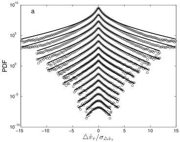
Fig. 1: Comparison of standardized PDFs of velocity increments $\triangle\hat{v}_{\tau}$ at different time scales (circles) with (a) the truncated stable distributions (lines) and (b) log-normal PDF model (lines). From top to bottom, time scales which range from $0.05$ s to $1638.4$ s increase as a geometric sequence with a common ratio of 2. The symbols $\sigma_{\triangle\hat{v}_{\tau}}$ is the standard deviation of $\triangle\hat{v}_{\tau}$. Plots have been arbitrarily shifted for illustration.

Standardized PDFs of $\triangle\hat{v}_{\tau}$ at different time scales are shown in Fig. 1. One can see that these PDFs are almost symmetrical and go from Gaussian like behavior at a time scale of more than ten minutes to some non-Gaussian behavior (with longer tails than Gaussian) at smaller time scales. This result is similar to that in Ref. [1] (see Fig. 4a in this article) where a longer time series (from 1960 to 1999) but with lower sampling frequency (1 hour) collected at the atmospheric boundary layer has been used. Moreover, this deformation behaviors of PDFs in the atmospheric turbulence are also similar to those observed in the local homogeneous and isotropic turbulence (see Fig. 4b in Ref. [1]). In the latter, it has long been recognized that the energy is transferred between various scales by the cascade process. It suggests that the energy transfer between atmospheric mesoscales and more smaller scales may be also related to some cascade process, although the turbulence at these scales is non-homogeneous and isotropic and is influenced by many factors like frictional drag, evaporation and transpiration, heat transfer, pollutant emission, terrain induced flow modification and so on [9].

In this study, two commonly used PDF models will be screened. One is the truncated stable distribution and the other is the log-normal PDF model. The truncated stable distribution was first proposed in Ref. [3] and then was used to account for the scaling behavior in the dynamics of an economic index [4]. After that, many other truncated stable distributions have been proposed [10, 11, 12, 13]. The distinction between these distributions is mainly focus on their tail distributions. In this research, we will focus on the one proposed in Ref. [10], which has the fewest tuning parameters and a smooth form at the same time. In Refs. [6, 7], this truncated stable distribution has been reported to fit the PDFs of atmospheric turbulent velocity. This distribution dose not have an analytical expression but has an analytical characteristic function $\Phi(k)$ [10]:

$$\ln\Phi(k) = \displaystyle\frac{\gamma^{\alpha}}{\cos(\pi\alpha/2)}\left\{\lambda^{\alpha}-(k^{2}+\lambda^{2})^{\alpha/2}\cos\left(\alpha\arctan\frac{k}{\lambda}\right)\right.$$ (4)

$$\displaystyle\left.\left[1-i\beta\tan\left(\alpha\arctan\frac{k}{\lambda}\right)\right]\right\},$$

when $0<\alpha<1$, and

$$\ln\Phi(k) = \displaystyle\frac{\gamma^{\alpha}}{\cos(\pi\alpha/2)}\left\{\lambda^{\alpha}-(k^{2}+\lambda^{2})^{\alpha/2}\cos\left(\alpha\arctan\frac{k}{\lambda}\right)\right.$$ (5)

$$\displaystyle\left[1-i\beta\tan\left(\alpha\arctan\frac{k}{\lambda}\right)\right]$$

$$-i\alpha\beta\lambda^{\alpha-1}k\bigg{\}},$$

when $1<\alpha<2$. Symbols $\alpha$, $\beta$, $\gamma$ and $\lambda$ represent four independent parameters which are normally obtained by fitting Eqs. (4) and (5) with the data. Equations (4) and (5) can be written in a simpler form [14]:

$$\ln\Phi(k)=C\Gamma(-\alpha)[q(\lambda+ik)^{\alpha}+p(\lambda-ik)^{\alpha}-\lambda^{\alpha}],$$ (6)

when $0<\alpha<1$, and

$$\ln\Phi(k)=C\Gamma(-\alpha)[q(\lambda+ik)^{\alpha}+p(\lambda-ik)^{\alpha}-\lambda^{\alpha}-i\alpha\lambda^{\alpha-1}(q-p)k],$$ (7)

when $1<\alpha<2$. The parameters are $C=-\gamma^{\alpha}/[\cos(\alpha\pi/2)\Gamma(-\alpha)]$, $p=(1+\beta)/2$ and $q=(1-\beta)/2$. For standardized and symmetrical PDFs, $\beta=0$ and [7]:

$$C\Gamma(-\alpha)\alpha\lambda^{\alpha-2}(\alpha-1)=1.$$ (8)

The log-normal model was originally proposed to account for the PDFs of velocity increments in the fully developed homogeneous and isotropic turbulence [2]. This model does not have an analytical PDF either. Its symmetrical PDF is:

$$f_{\tau}(\triangle\hat{v})=\frac{1}{2\pi\lambda_{\tau}}\int_{0}^{\infty}\exp\left(-\frac{\triangle\hat{v}^{2}}{2\sigma^{2}}\right)\exp\left(-\frac{\ln^{2}(\sigma/\bar{\sigma}_{\tau})}{2\lambda_{\tau}^{2}}\right)\frac{d\sigma}{\sigma^{2}},$$ (9)

where $\bar{\sigma}_{\tau}$ and $\lambda_{\tau}$ are parameters depending on scale $\tau$. For standardized PDF, there is only one independent parameter and the other parameter can be obtained by resolving the equation:

$$\bar{\sigma}_{\tau}^{2}\exp(2\lambda_{\tau}^{2})=1.$$ (10)

Figure 1 shows the comparison of experimental PDFs with above two models. Results show that the truncated stable distribution seems as “good” as the log-normal model when fitting to the data. They both fit to the experimental PDFs well except their far tails where the data seem to decay faster than the models with unknown reasons (see also Fig. 2 in Ref. [5], where a similar deviation from log-normal model has been observed). This reason may be physical, but also may be artificial. Due to the limited data, tail distributions may be underestimated. In short, by only fitting the PDFs we cannot say which model is better to account for the data. We also cannot say anything more about the underlying cascade process in the atmospheric turbulence. This is the motivation for us to look into the scaling behaviors in the atmospheric turbulence.

3 Scaling behavior

3.1 Probability of return

Probability of return is defined as the probability density at the origin for symmetrical probability density function (PDF). In the data analysis, a probability density defined on a small interval $(-h,h)$ can be used as an approximation of the probability of return:

$$f_{\tau}(\triangle\hat{v}=0)\approx f_{\tau}(-h<\triangle\hat{v}<h),$$ (11)

if the threshold $h$ is small enough. In Fig. 2, circles denote the probability of return of atmospheric turbulent velocity with a threshold of 0.01. At small scales, this function behaves as a power of time scales $\tau$:

$$f_{\tau}(\triangle\hat{v}=0)\propto\tau^{-p}.$$ (12)

A least-square fitting shows that the exponent $p\approx 0.2145$. For comparison, the probability of return of Gaussian distribution is also shown here:

$$G_{\tau}(0)=\frac{1}{\sqrt{2\pi}\sigma_{\tau}},$$ (13)

where the standard deviation $\sigma_{\tau}=\sigma_{\triangle\hat{v}_{\tau}}$. The difference between $f_{\tau}(\triangle\hat{v}=0)$ and $G_{\tau}(0)$ decreases with the increase of $\tau$, which implies a convergence to the gaussian distribution at large time scales. We also compute the probability of return with a much smaller threshold of 0.001 and find that above results do not change any more except that there are some statistical errors at large time scales and a little larger slope at small time scales.

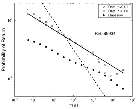
Fig. 2: Probability of return for the wind velocity increments as a function of time scales $\tau$ (circles for threshold $h=0.01$ and squares for $h=0.001$). For comparison, the probability of return for Gaussian distributions (see Eq. (13)) is also shown in this plot (black dots). The slope of the best-fit line (fitting data when $\tau<204.8$ s) is -0.2145 and the corresponding correlation coefficient is about 0.999. Broken line shows a power function with an exponent of -0.5.

3.2 Moments

Scaling behavior in the statistical moments of velocity increments (also called structure functions) is the central topic for the homogeneous and isotropic turbulence. Many theoretical works have devoted to the understanding of this scaling behavior and the underlying physical mechanisms [15]. For the non-homogeneous and non-isotropic atmospheric turbulence, its statistical moments also have scaling behavior at a wide range of time scales. Figure 3a shows the statistical moments of atmospheric turbulent velocity increments. One can see that at small time scales,

$$Z_{\tau,q}\equiv\overline{|\triangle\hat{v}_{\tau}|^{q}}\propto\tau^{\xi_{q}},$$ (14)

where the exponents $\xi_{q}$ vary as a function of $q$ (Fig. 3b). This power-law scaling behavior is observed for time intervals spanning three orders of magnitude for small values of $q$. However, for larger values of $q$ (for example, $q=2.5$ and $3$ in Fig. 3a) data begin to deviate from this scaling behavior at very small time scales ($\tau<1s$). The higher-order moments is mainly defined by the tail distributions which describe the statistical behavior of turbulent eddies with large characteristic velocities. It suggests that the relatively very small turbulent eddies with large characteristic velocities may have different cascade process from these eddies with larger scales. However, as already remarked in Fig. 1, all the conclusions about the tail distributions should be carefully screened because of the limited data.

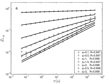
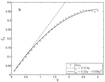
Fig. 3: (a) Scaling behavior of $q$th order moments $Z_{\tau,q}$. Lines represent the least-square fitting to Eq. (14) and the corresponding correlation coefficients $R$ are also listed. Grey points are not used in the fittings. (b) Scaling exponents $\xi_{q}$ vary as a function of $q$. Line shows the fitting result with the log-normal model and the broken one is a line through the origin with a slope of $p$, where $p$ is the scaling exponent of probability of return (see Eq. (12)).

Comparing with the exponents $\xi_{q}$ of homogeneous and isotropic turbulence [15], we found that $\xi_{q}$ of non-homogeneous and non-isotropic atmospheric turbulence are also concave but their values are much smaller. For the homogeneous and isotropic turbulence at high Reynolds number, the slope of $\xi_{q}$ at small values of $q$ is about $1/3$ and $\xi_{3}=1$ (Kolmogorov’s four-fifths law). As shown in Fig. 3b, the slope of $\xi_{q}$ at small values of $q$ in the atmospheric turbulence is about $1/5$ and $\xi_{3}\approx 0.35$. According to the Kolmogorov hypothesis in the log-normal model[16, 2],

$$9\lambda^{2}=\Lambda^{2}_{0}-\mu\ln\tau,$$ (15)

where $\Lambda_{0}$ and $\mu$ are parameters independent of $\tau$. For a fixed time scale, a smaller value of $\mu$ corresponds to a larger value of $\lambda$ which means that the tail of PDF becomes longer and the corresponding turbulence is more intermittent (see Eq. (9)). Following Eq. (15) and the assumption $\bar{\sigma}_{\tau}\propto\tau^{b}$, one can deduce that the exponents $\xi_{q}$ behave as a simple parabola:

$$\xi_{q}=bq-aq^{2},$$ (16)

where $b$ is some constant and $a=\mu/18$. A least-square fitting shows that $a\approx 0.04$ for atmospheric turbulence while this value is about 0.01 observed in the fully developed homogeneous and isotropic turbulence [15]. Thus, from the view of log-normal model and the Kolmogorov hypothesis the homogeneous and isotropic turbulence is less intermittent than the non-homogeneous and non-isotropic atmospheric turbulence.

4 Comparison with models

The truncated stable distribution and the log-normal model have different cascade processes which can cause the different scaling behaviors. The center part of truncated stable distribution at small scales behaves like a stable distribution with the same parameters $\alpha$, $\beta$ and $\gamma$. A notable feature of the stable distribution is its stability [17]:

$$\sum_{i=1}^{n}\triangle\hat{v}_{\tau_{0},i}\stackrel{{\scriptstyle d}}{{=}}n^{\frac{1}{\alpha}}\triangle\hat{v}_{\tau_{0}},$$ (17)

where $n$ is a positive integer and $\triangle\hat{v}_{\tau_{0},i}$ $(i=1,2,\cdots,n)$ are independent random variables with the same distribution as $\triangle\hat{v}_{\tau_{0}}$. The symbol “$\stackrel{{\scriptstyle d}}{{=}}$” means equality in distribution.

From Eq. (3), one can see that

$$\triangle\hat{v}_{\tau}=\sum_{i=1}^{n}\triangle\hat{v}_{\tau_{0},i},$$ (18)

where $\triangle\hat{v}_{\tau_{0},i}\equiv\hat{v}(t+i\tau_{0})-\hat{v}(t+(i-1)\tau_{0})$ and $n=\tau/\tau_{0}$. Thus, the truncated stable distribution contains a self-affine cascade process at small scales [8]:

$$\triangle\hat{v}_{\tau}\stackrel{{\scriptstyle d}}{{=}}n^{\frac{1}{\alpha}}\triangle\hat{v}_{\tau_{0}}.$$ (19)

An equivalent expression of Eq. (19) is

$$f_{\tau_{0}}(\triangle\hat{v})=n^{1/\alpha}f_{\tau}(n^{1/\alpha}\triangle\hat{v}).$$ (20)

From this expression, one can deduce that the probability of return for the truncated stable distribution behaves as a power of time scale:

$$f_{\tau}(\triangle\hat{v}=0)\propto\tau^{-1/\alpha}.$$ (21)

Although the probability of return of truncated stable distribution has a scaling behavior at small scales, one should note that the scaling exponent $1/\alpha\in[0.5,\infty)$. This scaling exponent is larger than that observed in the atmospheric turbulence (see Fig. 2). For the $q$th-order moments, authors (Refs. [14, 18]) have proved that the truncated stable distribution also has a scaling behavior but the scaling exponents vary as a bi-linear function of $q$:

$$\xi_{q}=\left\{\begin{array}[]{ll}q/\alpha,&(0<q<\alpha)\\ 1,&(q>\alpha)\\ \end{array}\right.$$ (22)

which is significantly different from the scaling exponents observed in the atmospheric turbulence, as shown in Fig. 3b.

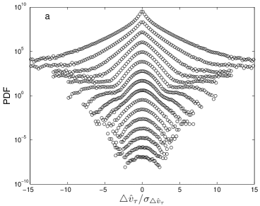
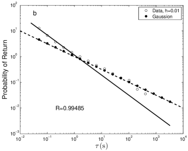
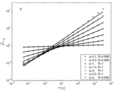
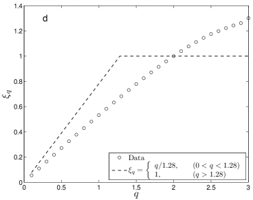
Fig. 4: Results for the surrogate wind velocity increments without correlations: (a) Standardized PDFs at different time scales. From top to bottom, the corresponding time scales are the same as those in Fig. 1. Plots are also arbitrarily shifted for illustration. (b) Probability of return with threshold $h=0.01$ (circles). The probability of return for Gaussian distribution (see Eq. (13)) is also shown here (black dots). The slope of the best-fit line (fitting data when $\tau<0.8$ s) is $-0.7808$ and the corresponding correlation coefficient is about $0.99$. Broken line shows a power function with an exponent of -0.5. (c) Scaling behavior of $q$-th order moments $Z_{\tau,q}$. All the symbols are the same as those in Fig. 3a. (d) Scaling exponents $\xi_{q}$ vary as a function of $q$. Broken lines shows a bi-linear function. The slope of this function is 0.7808 when $q<1/0.7808$ (see Eq. (22)).

In order to deduce Eq. (21), we have assumed that wind velocity increments in Eq. (17) are independent of each other . However, some correlations may exist among these increments. A direct proof comes from the scaling behavior of second-order moment. As shown in Fig. 3, the scaling exponent of second-order moment is obviously smaller than one, while for independent random variables this value equals to one. Correlation may be a possible reason that the scaling exponents of probability of return is smaller than the prediction of truncated stable distribution. To verify this speculation, we generate an independent time series by randomly sort the original time series of $\triangle\hat{v}_{\tau_{0}}$. This surrogate time series will have the same statistical distribution as the original time series. Independent surrogate time series at other larger scales can also be obtained by Eq. (3). We then compute the probability density functions of the surrogate time series at different time scales and find that with the increase of scales they approach Gaussian-like distributions much faster than the original time series (comparing Fig. 4a with Fig. 1). This is also proved in Fig. 4b, where the probability of return is almost the same as that of independent Gaussian distribution when time scale $\tau>1s$. Most importantly, one can see that the scaling exponent of probability of return is about 0.78 which falls on the range $[0.5,\infty)$ that the scaling exponent of truncated stable distribution belongs to. Thus, we can conclude that the correlation in the wind velocity increments is indeed a possible reason that the scaling exponent of probability of return deviates from the prediction of truncated stable distribution. However, this reason is not enough to account for the deviation of moments. For the surrogate time series, their exponents of moments $\xi_{q}$ is also a concave function of $q$, while the scaling exponents of truncated stable distribution obey a bi-linear behavior.

According to Eq. (9), the log-normal PDF model can be expressed by a simple random mapping:

$$\triangle\hat{v}_{\tau}\stackrel{{\scriptstyle d}}{{=}}W_{\bar{\sigma}_{\tau},\lambda_{\tau}}G,$$ (23)

where $W_{\bar{\sigma}_{\tau},\lambda_{\tau}}$ is a log-normal random variable and its logarithm has a mean of $\ln\bar{\sigma}_{\tau}$ and a standard deviation of $\lambda_{\tau}$. The symbol $G$ denotes a normally distributed random variable and is independent of $W_{\bar{\sigma}_{\tau},\lambda_{\tau}}$. For log-normal random variables, we have

$$W_{\bar{\sigma}_{\tau},\lambda_{\tau}}\stackrel{{\scriptstyle d}}{{=}}W_{\bar{\sigma}_{T},\lambda_{T}}W_{\bar{\sigma}_{\tau^{\prime}},\lambda_{\tau^{\prime}}},$$ (24)

where $W_{\bar{\sigma}_{T},\lambda_{T}}$ and $W_{\bar{\sigma}_{\tau^{\prime}}}$ are independent log-normal random variables, and $\ln\bar{\sigma}_{T}+\ln\bar{\sigma}_{\tau^{\prime}}=\ln\bar{\sigma}_{\tau}$ and $\lambda_{T}^{2}+\lambda_{\tau^{\prime}}^{2}=\lambda_{\tau}^{2}$. Based on Eq. (23) and Eq. (24), one can deduce that the log-normal PDF model has a cascade process:

$$\triangle\hat{v}_{\tau}\stackrel{{\scriptstyle d}}{{=}}W_{\bar{\sigma}_{T},\lambda_{T}}\triangle\hat{v}_{\tau^{\prime}}.$$ (25)

Comparing Eqs. (19) and (25), we find that the cascade process is very different between the truncated stable distribution and the log-normal PDF model. For the truncated stable distribution, the connection between different scales is a non-random power function which can only produce a stochastic process with scaling exponents $\xi_{q}$ of moments varying as a linear function of order $q$. This process is referred as a self-affine or self-similar fractal. To obtain a stochastic process with a non-linear scaling exponents of $\xi_{q}$ which is referred as a multifractal, one should extend the non-random power function to a random variable [8]. For the log-normal PDF model, the connection is a log-normally distributed random variable and it can produce a multifractal process by assuming suitable relationships between parameters ($\bar{\sigma}_{\tau}$, $\lambda_{\tau}$) and time scales $\tau$.

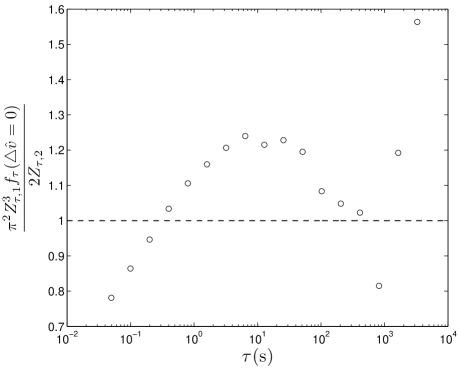
Fig. 5: Test of Eq. (29).

As we have mentioned in Sec. 3.2, under the assumptions of Eq. (15) and $\bar{\sigma}_{\tau}\propto\tau^{b}$, the scaling exponents $\xi_{q}$ of log-normal model vary as a parabola function (see Eq. (16)) and this function can fit the data well (see Fig. 3b). However, we will show that whatever the relationships between parameters ($\bar{\sigma}_{\tau}$, $\lambda_{\tau}$) and time scales are assumed the log-normal PDF model can not fit the probability of return and the moments at the same time. According to Eq. (9), the probability of return of log-normal PDF model is:

$$f_{\tau}(\triangle\hat{v}=0)=\frac{e^{\lambda_{\tau}^{2}/2}}{\sqrt{2\pi}\bar{\sigma}_{\tau}}$$ (26)

We can also deduce its $q$-order moment [2]:

$$Z_{\tau,q}={\bar{\sigma}_{\tau}}^{q}P_{q}\exp(q^{2}{\lambda_{\tau}}^{2}/2),$$ (27)

where

$$P_{q}=\displaystyle\frac{1}{\sqrt{2\pi}}\int_{-\infty}^{\infty}|x|^{q}\exp(-x^{2}/2)\,dx.$$ (28)

From Eqs. (26) and (27), we have:

$$\frac{\pi^{2}}{2}\frac{Z_{\tau,1}^{3}f_{\tau}(\triangle\hat{v}=0)}{Z_{\tau,2}}=1$$ (29)

In Fig. 5, one can see that the left-hand side of Eq. (29) is not a constant of one and varies as a function of $\tau$. Thus, we conclude that the log-normal PDF model can not fit the probability of return and the moments at the same time.

5 Conclusions

In this paper, we have shown the scaling behavior of the probability of return and the moments of atmospheric turbulent velocity increments. The probability of return is found to vary as a power function of time scale at smaller time scales. This scaling behavior is observed for time scales spanning three orders of magnitude, from 0.1s to 100s. The moments are also found to vary as a power function of time scales at smaller time scales. The scaling range can also spanning three orders of magnitude when the order of moment is not too large. However, with the increase of the order of moment the scaling range begins to shrink. Since the behavior of higher-order moments is mainly defined by tail distributions, the shrinkage may be caused by different cascade processes that the central and tail distributions represent. This conclusion should be carefully screened by using more data. Scaling exponents of moments vary as a concave function of order, which suggests that the time series of atmospheric turbulent velocity increments is a multifractal. Scaling exponents of moments observed in the homogeneous and isotropic turbulence are also concave but the values are obviously larger than those observed in the atmospheric turbulence.

The scaling behavior of the probability of return and the moments observed in the time series of atmospheric turbulent velocity increments is compared with the predictions of two commonly used PDF model, the truncated stable distribution and the log-normal PDF model. We find that both PDF models can not fit the probability of return and the moments at the same time. The truncated stable distribution can produce a power law of probability of return but the power exponent is too large to fitting the data. One possible reason is that the truncated stable distribution can only describe the independent random process while some statistical correlations always exist in the time series of atmospheric turbulent velocity increments. The truncated stable distribution can also produce a power law of moments. The power exponents vary as a bi-linear function of order, while the observed exponents are concave. The log-normal PDF model seems to be better than the truncated stable distribution. Under some conditions, its exponents vary as a parabola function which can fit the data well. However, this model can not fit the probability of return and the moments at the same time either.

Although above mentioned PDF models can not describe the scaling behavior in the atmospheric turbulence, they also give a clues that the scaling behavior may related to the cascade process of turbulent eddies. Our study may help in the understanding of the cascade mechanism in the atmospheric turbulence.

References

- Muzy et al. [2010] J. Muzy, R. Baïle, P. Poggi, Intermittency of surface-layer wind velocity series in the mesoscale range, Phys. Rev. E 81 (2010) 056308.
- Castaing et al. [1990] B. Castaing, Y. Gagne, E. Hopfinger, Velocity probability density functions of high Reynolds number turbulence, Physica D 46 (1990) 177.
- Mantegna and Stanley [1994] R. Mantegna, H. Stanley, Stochastic process with ultraslow convergence to a Gaussian: the truncated lévy flight, Phys. Rev. Lett. 73 (1994) 2946.
- Mantegna and Stanley [1995] R. Mantegna, H. Stanley, Scaling behaviour in the dynamics of an economic index, Nature 376 (1995) 46.
- Boettcher et al. [2003] F. Boettcher, C. Renner, H.-P. Waldl, J. Peinke, On the statistics of wind gusts, Boundary-Layer Meteorol. 108 (2003) 163.
- Liu et al. [2010] L. Liu, F. Hu, X.-L. Cheng, L.-L. Song, Probability density functions of velocity increments in the atmospheric boundary layer, Boundary-Layer Meteorol. 134 (2010) 243–255.
- Liu et al. [2011] L. Liu, F. Hu, X.-L. Cheng, Probability density functions of turbulent velocity and temperature fluctuations in the unstable atmospheric surface layer, J. Geophys. Res. 116 (2011) D12117.
- Mandelbrot [1997] B. Mandelbrot, A multifractal model of asset returns, Cowles Foundation Discussion Paper No. 1164 (1997).
- Stull [1988] R. Stull, An introduction to boundary layer meteorology, Kluwer Academic Publishers, Dordrecht, 1988.
- Koponen [1995] I. Koponen, Analytic approach to the problem of convergence of truncated lévy flights towards the Gaussian stochastic process, Phy. Rev. E 52 (1995) 1197–1199.
- Gupta and Campanha [1999] H. Gupta, J. Campanha, The gradually truncated Lévy flight for systems with power-law distributions, Physica A 268 (1999) 231–239.
- Gupta and Campanha [2000] H. Gupta, J. Campanha, The gradually truncated Lévy flight: stochastic process for complex systems, Physica A 275 (2000) 531–543.
- Matsushita et al. [2003] R. Matsushita, P. Rathie, S. D. Silva, Exponentially damped Lévy flights, Physica A 326 (2003) 544.
- Nakao [2000] H. Nakao, Multi-scaling properties of truncated Lévy flights, Phys. Lett. A 266 (2000) 282.
- Frisch [1995] U. Frisch, Turbulence, Cambridge University Press, Cambridge, 1995.
- Kolmogorov [1962] A. Kolmogorov, A refinement of previous hypotheses concernign the local structure of turbulence in a viscous incompressible fluid at high reynolds number, J. Fluid Mech. 13 (1962) 82–85.
- Nolan [2012] J. P. Nolan, Stable Distributions - Models for Heavy Tailed Data, Birkhauser, Boston, 2012. In progress, Chapter 1 online at http://academic2.american.edu/~jpnolan.
- Terdik et al. [2006] G. Terdik, W. Woyczynski, A. Piryatinska, Fractional- and integer- order moments, and multiscaling for smoothly truncated lévy flights, Phys. Lett. A 348 (2006) 94–109.